


Nomenclature
- c
-
chord
- C d
-
coefficient of drag
- C f
-
coefficient of skin friction
- C l
-
coefficient of lift
- C p
-
coefficient of pressure
- A
-
morphing angle
- L/D
-
lift-to-drag ratio
Greek symbol
- α
-
angle-of-attack
1.0 Introduction
The UAV sector has witnessed significant growth and is estimated to grow by more than 13% by 2022 [1]. Projections estimate the value of the UAV sector to be around US$30 billion dollars per year by 2035 [Reference Wargo, Church, Glaneueski and Strout2]. UAVs have been widely used for military reconnaissance, and there has been rising demand for civilian operations as well [Reference Wargo, Church, Glaneueski and Strout2]. With increasing carbon emissions in the aviation industry [Reference Zheng, Graver and Rutherford3], it is imperative to design fuel efficient vehicles to decrease carbon emissions. Since UAVs have attracted much attention and are also expected to grow significantly, it is important to improve the performance of such vehicles to reduce their fuel consumption. With recent advances in smart materials, sensors and actuators [Reference Körpe and özgen4], morphing wing technology is seen as a viable option to improve the performance of UAVs. Interestingly, morphing has been adapted in Nature by flying species such as bats to increase their aerodynamic performance [Reference Yu and Guan5].
A morphing aircraft has the capability to alter its shape during flight to achieve optimum performance [Reference Barbarino, Bilgen, Ajaj, Friswell and Inman6]. Extensive reviews of various morphing wing methodologies have been presented by Barbino et al. [Reference Barbarino, Bilgen, Ajaj, Friswell and Inman6] and Sofla et al. [Reference Sofla, Meguid, Tan and Yeo7]. One such methodology is camber morphing. The earliest work on camber morphing dates back to 1920, when Parker [Reference Parker8] patented one of the earliest models for a variable-camber morphing wing. Since then, camber morphing has received considerable attention over the years, especially due to progress in the development of camber-changing mechanisms and actuation technologies. An objective of camber morphing is to smoothly deform the camberline to increase the effective camber, resulting in the generation of additional lift. Smoothly varying the camberline by camber morphing can eliminate discontinuities, thereby reducing the tendency for flow separation. As a result, the aerodynamic performance obtained through camber morphing is relatively higher when compared with devices such as the trailing-edge flap. Naranjo et al. [Reference García Naranjo, Cowling, Green and Qin9] investigated the effect of the maximum camber and its position on the aerodynamic parameters. They concluded that aerofoil profiles with 6–8% camber at 60% chord position exhibit the highest lift-to-drag ratio, suggesting an increased range for the aircraft and the highest endurance factor, and thus a reduced propulsive power requirement. The Fishbone Active Camber (FishBAC) for morphing wings was proposed by Woods and Friswell [Reference Woods and Friswell10]. Aerofoils employing the FishBAC concept have been found to display reduced drag as well as enhanced aerodynamic performance [Reference Woods, Fincham and Friswell11]. The aerodynamic performance was found to depend on the starting location of the morphing. More recently, Wu et al. [Reference Wu, Soutis, Zhong and Filippone12] introduced a camber morphing mechanism actuated by Linear UltraSonic Motors (LUSMs) to expand the flight envelope of UAVs. Chanzy and Keane [Reference Chanzy and Keane13] designed a small UAV employing camber morphing to achieve roll control. They reported that the modified UAV exhibited a lower roll rate and significantly higher performance compared with a UAV with conventional wings. Zhang et al. [Reference Zhang, Ge, Zhang, Mo and Zhang14] investigated the effect of compliant mechanism-based leading- and trailing-edge morphing on the aerodynamic characteristics. It was found that the lift and drag coefficients were less sensitive to leading-edge morphing when compared with trailing-edge morphing. The mechanism was also found to resist deformation due to aerodynamic loads. Sahin et al. [Reference Şahin, Çakır and Yaman15] employed a scissor-structural mechanism (SSM) to morph baseline NACA four-digit aerofoils into other aerofoils of the same family that have a different maximum camber percentage. The mechanism was able to satisfy the target aerofoil profiles with a little compensation in lift. Aerostructural optimisation performed on a shape-memory alloy-actuated morphing wing by Leal et al. [Reference Leal, Savi and Hartl16] achieved a 22% weight reduction and an increase of the stall angle. Apart from their application on wings, camber morphing has also be investigated for other components to improve their aerodynamic performance. Camber morphing of winglets was found to improve the fuel efficiency of business jets, as reported by Eguea et al. [Reference Eguea, Pereira Gouveia da Silva and Martini Catalano17]. Ferede and Gandhi [Reference Ferede and Gandhi18] found that camber morphing of the blade tips of wind turbines could alleviate fatigue loads by between 8% and 37%.
Although morphed aircraft offer several advantages such as improved performance, lower fuel consumption and reduced structural weight (by removing the complex mechanisms of ailerons and flaps) [Reference Woods and Friswell19], they are associated with various practical issues. The major problem with morphing wing structures is the conflicting requirements for the structure to be both stiff enough to take large aerodynamic loads but simultaneously flexible enough to deform as desired. A corrugated structure composed of a wavy plate [Reference Yokozeki, Takeda, Ogasawara and Ishikawa20] is a promising candidate for variable-camber morphing wings. Research pertaining to analysis of corrugated structures over recent years has produced results that favour their use for morphing applications [Reference Takahashi, Yokozeki and Hirano21–Reference Kumar, Faruque Ali and Arockiarajan23]. Corrugated structures have small stiffness along the axial direction, thereby allowing suitable axial deformations under low actuation loads. Meanwhile, the large magnitude of the stiffness along the transverse direction allows the structure to withstand aerodynamic loads. This paper investigates the aerodynamic characteristics of the NACA0012 aerofoil with single corrugated structures to achieve camber morphing. The aerodynamic characteristics are obtained from two different Computational Fluid Dynamics (CFD) solvers and a panel code. The results from the aerodynamic analysis are compared, and the effect of camber morphing on aerodynamic efficiency parameters such as the lift-to-drag ratio and endurance factor is investigated.
Table 1. Geometrical parameters of the aerofoil and corrugated structure considered in this study
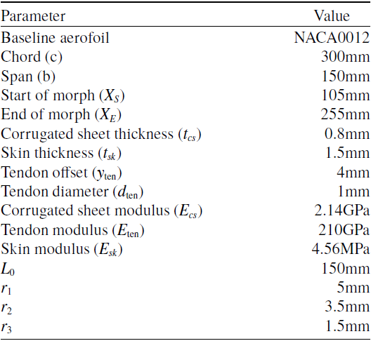
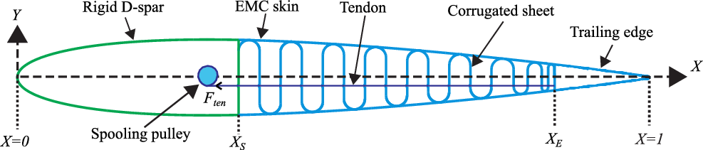
Figure 1. The morphing aerofoil configuration composed of a single corrugated structure.
2.0 Methodology
2.1 Structural analysis
The study by Yokozeki et al. [Reference Yokozeki, Takeda, Ogasawara and Ishikawa20] on morphing wings indicated that corrugated structures comprising a wavy plate represent a suitable choice for morphing wings as they can withstand large spanwise lift loads but still exhibit high flexibility due to their highly anisotropic stiffness. In the present work, a Single Corrugated Variable-Camber (SCVC) morphing aerofoil concept is adapted for morphing the aerofoil [Reference Yokozeki, Takeda, Ogasawara and Ishikawa20,Reference Takahashi, Yokozeki and Hirano21,Reference Yokozeki, Aya and Yoshiyasu24,Reference Tsushima, Yokozeki, Su and Arizono25], as shown in Fig. 1. The morphing section of the wing consists of a single corrugated structure which extends from $X_{S} = 0.35c$
to
$X_{S} = 0.35c$
to $X_{E} = 0.85c$
. The envelope of the corrugation coincides with the shape of aerofoil (NACA0012) and is connected to a pre-tensioned Elastomeric Matrix Composite (EMC) skin surface (Fig. 1). To create smooth and large changes in the aerofoil camber, a high-stiffness tendon with a spooling pulley is mounted. The corrugated structure is made of Acrylonitrile Butadiene Styrene (ABS) plastic. The geometric and material parameters of the model are presented in Table 1. The deflected profiles of the present configuration are obtained by an analytical method using chain calculations and a commercial finite-element solver ABAQUS [27]. Geometric and elastic linear deformation theory is assumed in both analyses.
$X_{E} = 0.85c$
. The envelope of the corrugation coincides with the shape of aerofoil (NACA0012) and is connected to a pre-tensioned Elastomeric Matrix Composite (EMC) skin surface (Fig. 1). To create smooth and large changes in the aerofoil camber, a high-stiffness tendon with a spooling pulley is mounted. The corrugated structure is made of Acrylonitrile Butadiene Styrene (ABS) plastic. The geometric and material parameters of the model are presented in Table 1. The deflected profiles of the present configuration are obtained by an analytical method using chain calculations and a commercial finite-element solver ABAQUS [27]. Geometric and elastic linear deformation theory is assumed in both analyses.
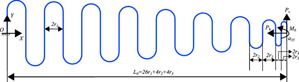
Figure 2. Schematic of the cantilever single corrugated structure under the action of end point loads.
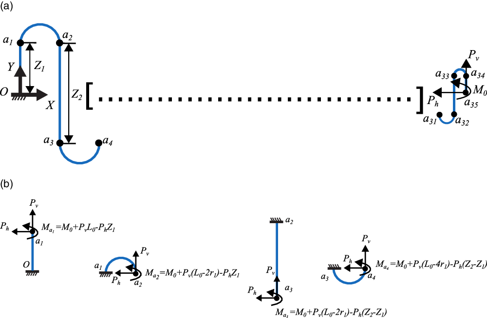
Figure 3. (a) Corrugated structure with cantilever boundary condition and point loads applied at free end $a_{35}$
. (b) Free body diagrams of individual beams with equivalent forces at the free end.
$a_{35}$
. (b) Free body diagrams of individual beams with equivalent forces at the free end.
2.1.1 Deflections of the single corrugated structure due to end loads using chain calculation
The present wing configuration is uniform in the span direction, thus a two-dimensional model is constructed. The compliant part of the morphing wing, which is a cantilever single corrugated structure with end loads, is shown in Fig. 2. The part of the aerofoil after the rigid D-spar is considered in the analytical model. The corrugated structure is fixed at the end O and loads ( $P_h, P_v, M_0$
) are applied at the free end
$P_h, P_v, M_0$
) are applied at the free end $a_{35}$
. The geometric parameters considered are presented in Table 1.
$a_{35}$
. The geometric parameters considered are presented in Table 1.
Figure 3 shows the discretisation of the corrugated structure and the free body diagrams of individual constituent beam elements with equivalent loads at the free ends. The corrugated structure shown in Fig. 3(a) is split into several straight ( $O{a_1}, {a_2}{a_3},...,{a_{34}}a_{35}$
) and semicircular beams (
$O{a_1}, {a_2}{a_3},...,{a_{34}}a_{35}$
) and semicircular beams ( ${a_1}{a_2}, {a_3}{a_4},...,{a_{33}}a_{34}$
). These beams are considered to be cantilever beams fixed to the end of the previous beam like chain links [Reference Kumar, Faruque Ali and Arockiarajan23]. The equivalent loads are calculated using static equilibrium for each beam (Fig. 3(b)). The deflections of each beam are then obtained by applying Euler–Bernoulli beam theory [Reference Gere and Timoshenko28], considering small deformations. The deflected profile of the corrugated structure is then obtained by combining the deflected shapes of each of the beams, maintaining continuity at the joints.
${a_1}{a_2}, {a_3}{a_4},...,{a_{33}}a_{34}$
). These beams are considered to be cantilever beams fixed to the end of the previous beam like chain links [Reference Kumar, Faruque Ali and Arockiarajan23]. The equivalent loads are calculated using static equilibrium for each beam (Fig. 3(b)). The deflections of each beam are then obtained by applying Euler–Bernoulli beam theory [Reference Gere and Timoshenko28], considering small deformations. The deflected profile of the corrugated structure is then obtained by combining the deflected shapes of each of the beams, maintaining continuity at the joints.
To clarify the proposed chain calculation, the logic is described through the flowchart shown in Fig. 4. For each node (free end of beams), the equivalent loads ( $P_h, P_v, M_{i}$
, where
$P_h, P_v, M_{i}$
, where $i=a_1,a_2,...,a_{35}$
) are calculated by transferring the free end load to each node. The Euler–Bernoulli beam model is then used to obtain the deflected profile of each beam. Then, compatibility conditions are applied to the free end of each beam. This procedure is continued until the last beam
$i=a_1,a_2,...,a_{35}$
) are calculated by transferring the free end load to each node. The Euler–Bernoulli beam model is then used to obtain the deflected profile of each beam. Then, compatibility conditions are applied to the free end of each beam. This procedure is continued until the last beam $(N=35)$
is reached.
$(N=35)$
is reached.
Figure 4. Flowchart for obtaining the deflected profile of the single corrugated structure.
2.1.2 Deflections of the single corrugated structure with an EMC skin under uniformly varying (triangular distribution) load and end point loads
In this subsection, the formulation for the single corrugated structure with an EMC skin subjected to a uniformly varying load and end point loads is presented. As the structure with skin is morphed down, the pretension in the bottom skin segments is released while the top skin segments are stretched further. Under this condition, where the skin is always in tension irrespective of whether it is at the bottom or top side, the EMC skin can be treated as pre-stretched springs which are capable of taking only axial loads.
Figure 5. Schematic of the single corrugated structure with EMC skin, modelled as axial spring elements subjected to uniformly varying load and end point loads.
Figure 5 shows the cantilevered corrugated structure where the EMC skin is replaced with axial spring elements subjected to uniformly varying load (q) and end point loads $(P_h,P_v,M_0)$
. The skin segments between two semicircles is modelled as spring elements with axial stiffness calculated as
$(P_h,P_v,M_0)$
. The skin segments between two semicircles is modelled as spring elements with axial stiffness calculated as $K_i=\frac{E_{sk}A}{L_i}$
, where
$K_i=\frac{E_{sk}A}{L_i}$
, where $E_{sk}$
is the skin modulus,
$E_{sk}$
is the skin modulus, $A_{sk}$
is the cross-sectional area of the skin,
$A_{sk}$
is the cross-sectional area of the skin, $L_i$
is the length of the
$L_i$
is the length of the $i^{\rm th}$
skin segment and
$i^{\rm th}$
skin segment and $i=1,2,3,...,18$
. The uniformly varying load present over the top skin surface is converted into equivalent forces and moments (
$i=1,2,3,...,18$
. The uniformly varying load present over the top skin surface is converted into equivalent forces and moments ( $F_1,M_1,F_2,M_2,...,F_9,M_9$
) to be applied at the points of attachment of the skin to the corrugated structure, as shown in Fig. 5. The equivalent load for the
$F_1,M_1,F_2,M_2,...,F_9,M_9$
) to be applied at the points of attachment of the skin to the corrugated structure, as shown in Fig. 5. The equivalent load for the $j^{\rm th}$
unit is calculated by integrating the force distribution between the
$j^{\rm th}$
unit is calculated by integrating the force distribution between the $j^{\rm th}$
and
$j^{\rm th}$
and $(j+1)^{\rm th}$
unit. This load is then transfer as force and moment (
$(j+1)^{\rm th}$
unit. This load is then transfer as force and moment ( $F_j,M_j$
) to the free end of the
$F_j,M_j$
) to the free end of the $j^{\rm th}$
unit.
$j^{\rm th}$
unit.
Figure 6. Geometry of the cantilever single corrugated structure with skin only on top surface under the action of uniformly varying load and end point loads. (a) Splitting of single corrugated structure into ten units with spring elements. (b) Unit 1 with spring force. (c) Unit 3, which is repeated, with spring force.
Figure 7. Flowchart for obtaining the deflected profile of single corrugated structure with EMC skin.
2.1.3 Deflections of the single corrugated structure with EMC skin on top surface
Figure 6 shows the single corrugated structure with skin only on the top surface, modelled as spring elements subjected to uniformly varying load and end point loads. The structure is divided into ten corrugated units, as shown in Fig. 6(a). Unit 1 is a quarter-circle with one spring element, and unit 3 consists of two straight and three curved beams along with one spring element, which is repeated to generate the single corrugated structure (Fig. 6(b) and (c)). The end point loads for each unit are calculated by considering the effects of the loads ( $P_h, P_v, M_0$
) at the end of the corrugated structure, the equivalent loads (
$P_h, P_v, M_0$
) at the end of the corrugated structure, the equivalent loads ( $F_j$
and
$F_j$
and $M_j$
) due to the uniformly varying force and the forces exerted by the spring elements. The line of action of spring forces will be co-linear with the line joining the fixed and free end of each unit with an inclination of
$M_j$
) due to the uniformly varying force and the forces exerted by the spring elements. The line of action of spring forces will be co-linear with the line joining the fixed and free end of each unit with an inclination of $\alpha_i$
with respect to the X-axis.
$\alpha_i$
with respect to the X-axis.
As the structure deforms due to the end loads, there will be a change in the length of spring element, which will exert a restoring force $F_{sj}=-K_j \Delta L{j}$
. Since the spring force depends on the change in length of the spring element, which is a function of the end point co-ordinates of the corrugated unit, this is solved iteratively. The Aitken relaxation technique [Reference Irons and Tuck26] is used to reduce the occurrence of large divergent oscillations in the predicted displacements between iterations. Relaxation techniques work by adding numerical damping to the solution, whereby the solution is only partially moved toward the solution predicted for the next iteration. In this way, the change in spring force is reduced, and the tendency of solutions to diverge is reduced. These techniques are particularly important for systems with large differences in the stiffness of the various components. In the case of the corrugated structure, the stiffness change between the straight beams and curved beams is significant, making relaxation essential for stability. The iterative solution is explained using the flowchart shown in Fig. 7. The convergence is achieved when the error,
$F_{sj}=-K_j \Delta L{j}$
. Since the spring force depends on the change in length of the spring element, which is a function of the end point co-ordinates of the corrugated unit, this is solved iteratively. The Aitken relaxation technique [Reference Irons and Tuck26] is used to reduce the occurrence of large divergent oscillations in the predicted displacements between iterations. Relaxation techniques work by adding numerical damping to the solution, whereby the solution is only partially moved toward the solution predicted for the next iteration. In this way, the change in spring force is reduced, and the tendency of solutions to diverge is reduced. These techniques are particularly important for systems with large differences in the stiffness of the various components. In the case of the corrugated structure, the stiffness change between the straight beams and curved beams is significant, making relaxation essential for stability. The iterative solution is explained using the flowchart shown in Fig. 7. The convergence is achieved when the error, $E_0$
, in the magnitude of tip displacement between two successive iterations is less than
$E_0$
, in the magnitude of tip displacement between two successive iterations is less than $10^{-4}$
.
$10^{-4}$
.
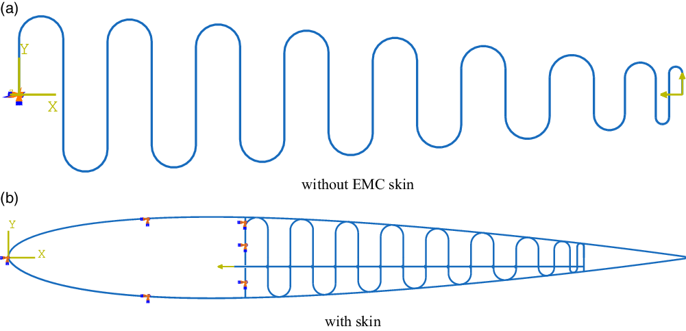
Figure 8. SCVC morphing wing modelled using FEA in ABAQUS®.
2.1.4 Finite-element analysis of SCVC morphing aerofoil
A finite-element analysis is carried out considering small deflection in ABAQUS®. Single corrugated structures with and without EMC skin are simulated in ABAQUS®, as shown in Fig. 8(a) and (b), respectively. For static analysis, the structures are discretised using two-node cubic beam elements in a plane (B23) for the SCVC model. Boundary conditions for both the models and the concentrated forces applied to the tendon wire are shown in Fig. 8(a) and (b). The material is assumed to exhibit linear elastic behaviour. The geometric properties of the FEA models are presented in Table 1.
2.1.5 Shape preservation study
The single corrugated structure uses its flexibility to achieve camber morphing of the original aerofoil via pulling the steel tendon. The morphed profile of the aerofoil is dictated by the relation between the structure’s stiffness distribution, actuation force and aerodynamic load. This implies that, for various speed and angle-of-attack combinations, the structure which is morphed to a particular trailing-edge displacement may adopt different camber profiles from the start of morphing to the trailing edge, as it will experience different aerodynamic loads. The ability of the structure to adopt the same shape for a chosen trailing-edge displacement irrespective of the aerodynamic loads acting on it is called its shape preservation capacity. In other words, depending on the aerodynamic loads, the actuation force required for a specific trailing-edge displacement can vary but the profile must remain the same. In case of 100% shape preservation, the aerodynamic performance of the morphed profiles can be studied without resorting to quasi-static FSI analysis. However, this property is directly dependent on the structure’s stiffness distribution, and in this paper a suitable corrugation thickness has been chosen to accomplish shape preservation, which enables us to neglect the structural effects of wind loads.
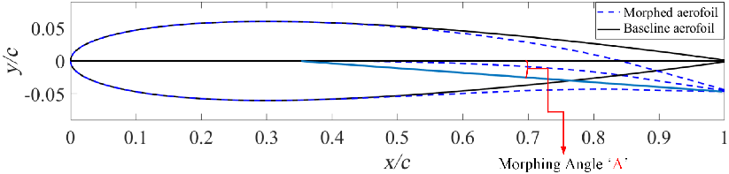
Figure 9. Representation of morphing angle.
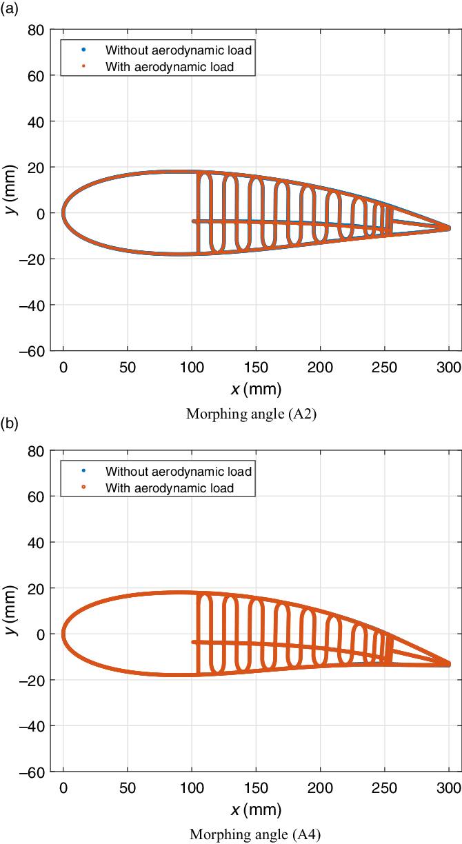
Figure 10. Shape comparison of SCVC model with and without aerodynamic loads.
To quantify the various degrees of morphing, a parameter called the morphing angle A is introduced. This is the angle between the straight line connecting the start of morphing (location) to the trailing edge of the morphed aerofoil and the chord line of the baseline aerofoil, as illustrated in Fig. 9. In this study, the morphing angle is varied from $2^\circ$
to
$2^\circ$
to $12^\circ$
in increments of
$12^\circ$
in increments of $2^\circ$
for the SCVC aerofoil.
$2^\circ$
for the SCVC aerofoil.
Figure 10 shows that the deformed shapes of the SCVC model with and without aerodynamic loads match well for two different morphing angles (A2 and A4). The aerodynamic coefficients computed using XFoil are also compared for these cases, as given in Table 2, and are found to be in good agreement.
Mean camber lines are calculated from the deformed aerofoils to generate the aerofoil surface using a numerical method, as discussed in the next subsection.
2.2 Aerofoil surface generation
The morphed camber lines extracted from the structural analysis are used to construct the aerofoil surface to determine their aerodynamic characteristics. NACA four- and five-digit aerofoils have theoretical equations for the thickness distribution, which can be added to the camber line to regenerate the aerofoil surface. This equation has been utilised by Woods et al. [Reference Woods, Fincham and Friswell11] to generate the surface of a morphed NACA0012 aerofoil. In the case of NACA six- and seven-digit aerofoils though, the thickness distribution equations are complex, making the generation of the aerofoil surface using these equations an arduous task. Consequently, numerical methods can be used to generate these aerofoil surfaces, despite the complexity in the thickness distribution along the aerofoil. Although this work focuses on the NACA0012 aerofoil, for which a relatively simpler thickness distribution function is available, the authors make use of a numerical method in this work that could, in principle, be applied for any given aerofoil.
The numerical approach used in this work is based on the framework adopted by Fincham and Friswell [Reference Fincham and Friswell29]. In this approach, the aerofoil surface is discretised as a cloud of points and radial basis functions are used to interpolate the changes in the surface owing to changes of the camber line, which is also represented by a point cloud. A study by Rendall and Allen [Reference Rendall and Allen30] revealed that the Radial Basis Function (RBF) method can be beneficial owing to the fact that points in the cloud can be of any spatial resolution and have any order. The accuracy of this approach depends on the number of surface control points (which form a subset of the aerofoil surface points), as the effect of the camber change is translated to changes in the surface control points, which in turn bring about the corresponding changes in the aerofoil surface. An optimal control-point count is required, since fewer points can lead to substantial errors in the generated profile while a large point count can be computationally expensive. The error estimate used here is the Root Mean Square (RMS) of the distances between the surfaces generated through the RBF [Reference Fincham and Friswell29] and thickness distribution functions. Figure 11 shows the variation of the error with the number of surface control points.
As seen from this figure, convergence occurs when the surface control point count is at least 40. Therefore, this point count is adopted for the rest of this work. It is observed though that the error converges to a value of about 0.002, which is about 0.2% of chord.
A comparison of the aerofoil surfaces generated using the RBF method and the thickness distribution function for the A4 aerofoil is shown in Fig. 12(a). Furthermore, a comparison of the drag polar (obtained from XFoil) for the aerofoils is also presented in Fig. 12(b). It is seen that the RBF method produces an aerofoil surface that is virtually identical to the surface generated using the thickness distribution approach and that also exhibits identical aerodynamic characteristics.
Table 2. Comparison of aerodynamic coefficients obtained using XFoil for the case without and with aerodynamic load on the SCVC model
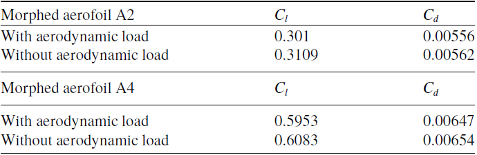
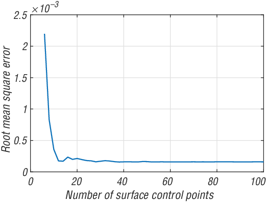
Figure 11. Variation of surface reconstruction error with respect to number of surface control points.
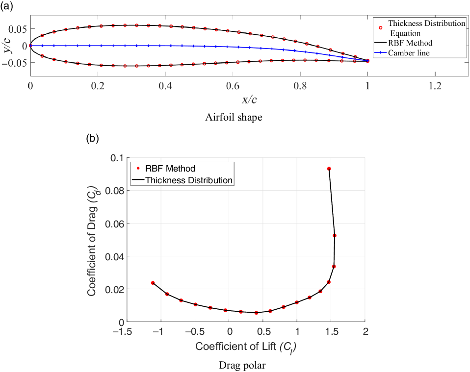
Figure 12. Comparison of aerofoils generated using RBF [Reference Fincham and Friswell29] and thickness distribution approach.
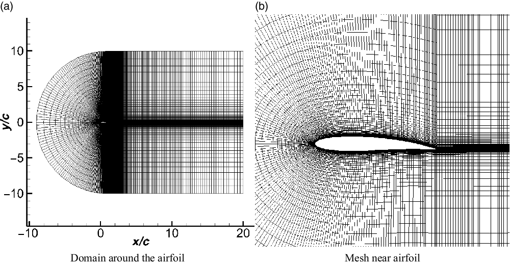
Figure 13. C-type mesh.
2.3 Aerodynamic analysis
To investigate the aerodynamic characteristics of the morphed aerofoils, two different CFD solvers (ANSYS Fluent and OpenFOAM) are employed in this study. A C-type structured mesh as shown in Fig. 13 is used for the baseline as well as morphed configurations. The C segment measures 10c in radius, and the rectangular block measures $20c \times 20c$
, where
$20c \times 20c$
, where $c = 1$
m is the chord length of the aerofoil.
$c = 1$
m is the chord length of the aerofoil.
For the CFD simulations, the flow over the aerofoil is considered to be turbulent; Menter’s $k-\omega$
Shear Stress Transport (SST) model is used as it is known to accurately predict flow separation in the presence of adverse pressure gradients [Reference Bardina, Huang and Coakley31,Reference Menter32]. An average
$k-\omega$
Shear Stress Transport (SST) model is used as it is known to accurately predict flow separation in the presence of adverse pressure gradients [Reference Bardina, Huang and Coakley31,Reference Menter32]. An average $y^+$
$y^+$ $\approx$
1 is maintained for the first layer of mesh nodes over the aerofoil to accurately resolve the turbulent boundary layer. A second-order-accurate reconstruction is employed for the momentum, turbulent kinetic energy and dissipation terms, and the SIMPLE algorithm is used for the solution of the discretised equations. THe freestream velocity is set to 14.6m/s, corresponding to a chord-based Reynolds number of 1
$\approx$
1 is maintained for the first layer of mesh nodes over the aerofoil to accurately resolve the turbulent boundary layer. A second-order-accurate reconstruction is employed for the momentum, turbulent kinetic energy and dissipation terms, and the SIMPLE algorithm is used for the solution of the discretised equations. THe freestream velocity is set to 14.6m/s, corresponding to a chord-based Reynolds number of 1 $\times$ $10^6$
, and the inflow turbulence intensity is fixed to be 1%. The angle-of-attack (
$10^6$
, and the inflow turbulence intensity is fixed to be 1%. The angle-of-attack ( $\alpha$
) is varied for each case such that the generated coefficient of lift (
$\alpha$
) is varied for each case such that the generated coefficient of lift ( $C_l$
) lies approximately in the range 0–1.3. This
$C_l$
) lies approximately in the range 0–1.3. This $C_l$
range represents the flight phase in UAVs as reported by Nickol et al. [Reference Nickol, Guynn, Kohout and Ozoroski33]. The
$C_l$
range represents the flight phase in UAVs as reported by Nickol et al. [Reference Nickol, Guynn, Kohout and Ozoroski33]. The $\alpha$
range for all cases is presented in Table 3.
$\alpha$
range for all cases is presented in Table 3.
Three different sets of boundary conditions are used for zero, positive and negative angles of attack. For $\alpha = 0^\circ$
, the C portion of the boundary and the upper and lower boundaries of the rectangular block are set to velocity inlet boundary condition while the right boundary is made a pressure outlet. When
$\alpha = 0^\circ$
, the C portion of the boundary and the upper and lower boundaries of the rectangular block are set to velocity inlet boundary condition while the right boundary is made a pressure outlet. When $\alpha > 0^\circ$
, a velocity inlet boundary condition is imposed on the C boundary of the mesh and lower boundary of the rectangular block, while pressure outlet boundary conditions are imposed on the upper and right boundaries. For cases with
$\alpha > 0^\circ$
, a velocity inlet boundary condition is imposed on the C boundary of the mesh and lower boundary of the rectangular block, while pressure outlet boundary conditions are imposed on the upper and right boundaries. For cases with $\alpha < 0^\circ$
, a velocity inlet boundary condition is imposed on the C portion and the upper boundary of the rectangular block, while pressure outlet boundary conditions are imposed on the right and lower boundaries. The boundary conditions for zero, positive and negative angles of attack are shown in Fig. 14. In all cases, no-slip condition is imposed on the aerofoil surface. A convergence criterion of
$\alpha < 0^\circ$
, a velocity inlet boundary condition is imposed on the C portion and the upper boundary of the rectangular block, while pressure outlet boundary conditions are imposed on the right and lower boundaries. The boundary conditions for zero, positive and negative angles of attack are shown in Fig. 14. In all cases, no-slip condition is imposed on the aerofoil surface. A convergence criterion of $10^{-6}$
is set for all the computed residuals. A total of five different meshes are made for the baseline NACA0012 aerofoil to perform the grid independence study. CFD simulation using Fluent is done at
$10^{-6}$
is set for all the computed residuals. A total of five different meshes are made for the baseline NACA0012 aerofoil to perform the grid independence study. CFD simulation using Fluent is done at $\alpha = 0^\circ$
for all the grids, and the
$\alpha = 0^\circ$
for all the grids, and the $C_d$
results are plotted in Fig. 15. As seen from this figure, the fourth grid comprising nearly 68,755 cells seems to give a result identical to the most refined mesh and is thus chosen for the rest of this study.
$C_d$
results are plotted in Fig. 15. As seen from this figure, the fourth grid comprising nearly 68,755 cells seems to give a result identical to the most refined mesh and is thus chosen for the rest of this study.
Table 3. Angle-of-attack ( $\alpha$
) range for SCVC aerofoil
$\alpha$
) range for SCVC aerofoil

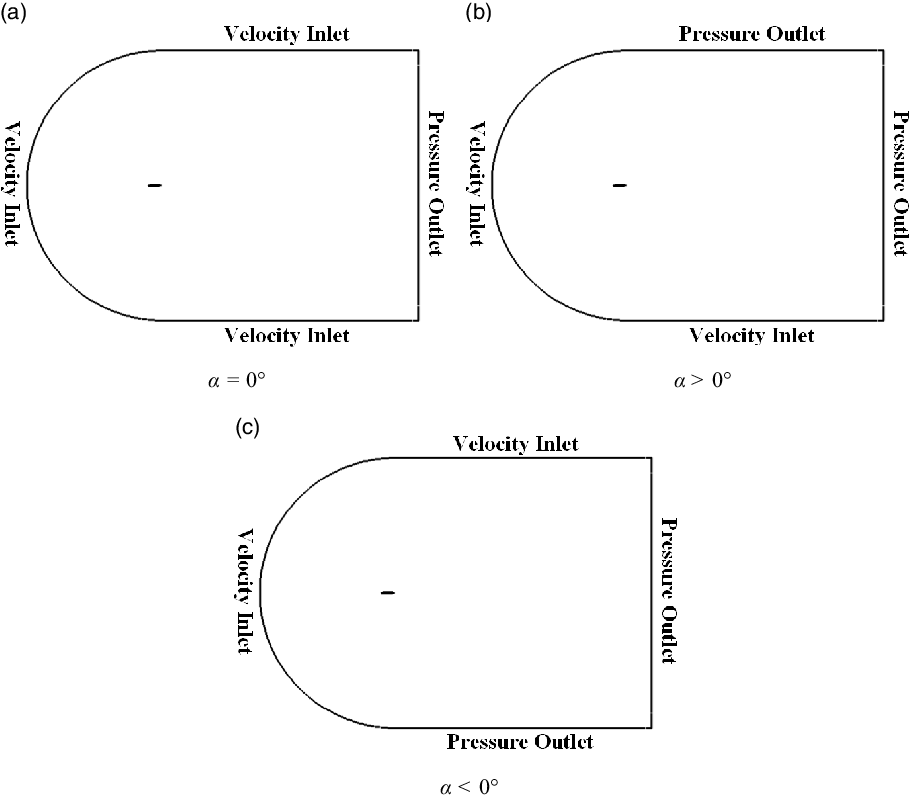
Figure 14. Boundary conditions.
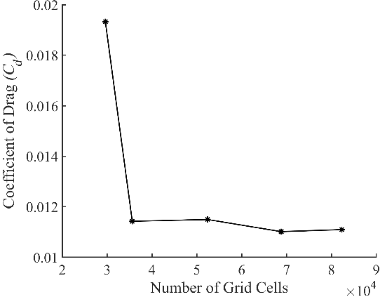
Figure 15. Grid convergence study.
In this study, a panel method (XFoil)-based analysis is also incorporated, as previous studies(11,34) indicate that prediction of aerodynamic coefficients by low-fidelity tools is comparable to their prediction by high-fidelity tools at low angles of attack. As such, this study also attempts to compare the results of XFoil and CFD analysis to explore the possibility of replacing high-fidelity tools with low-fidelity tools for morphed aerofoils in view of reduced computational costs. Viscous effects in XFoil are realised using a two-equation lagged dissipation integral method, and the transition is predicted using the $e^N$
method [Reference Drela and Giles36]. While the CFD results assume fully turbulent flow, the XFoil analysis incorporates flow transition.
$e^N$
method [Reference Drela and Giles36]. While the CFD results assume fully turbulent flow, the XFoil analysis incorporates flow transition.

Figure 16. Deformed profiles of single corrugated structure due to end loads.
3.0 Results and Discussion
A validation of the structural model is presented first, followed by a validation of the numerical methods (for computational aerodynamics) against aerofoil experimental data. Thereafter, the morphed aerofoil configurations are compared with the baseline aerofoil for a $C_l$
range [0, 1.3] to identify the effect of morphing on the lift-to-drag ratio and endurance factor. The range of lift coefficient is chosen such that it represents the entire flight regime [Reference Nickol, Guynn, Kohout and Ozoroski33]: take-off/landing, loiter and dash of a UAV.
$C_l$
range [0, 1.3] to identify the effect of morphing on the lift-to-drag ratio and endurance factor. The range of lift coefficient is chosen such that it represents the entire flight regime [Reference Nickol, Guynn, Kohout and Ozoroski33]: take-off/landing, loiter and dash of a UAV.
3.1 Validation of structural model
To establish the accuracy of the proposed structural model, the results are compared with the ABAQUS® solution with and without EMC skin for various loading conditions. The deflected profiles of the corrugated structure are shown in Figs 16 and 17. Two loading cases are considered for comparison of the structure without skin: Load-1 and Load-2, and three loading cases for the structure with skin: Load-3, Load-4 and Load-5, as described in Table 4 and 5, respectively. Figures 16 and 17 show that the results obtained from the proposed method match very closely with those obtained using ABAQUS® for all load cases.
The proposed structural model is written in MATLAB® [37] (facilitating integration and geometry definition) and allows for significantly faster analysis of the single corrugated structure with distributed loading than when using ABAQUS®. The deformed shapes and camber lines of the morphed aerofoil for different morphing angles (A2, A6 and A10) obtained from the structural analysis are shown in Fig. 18 for the applied tendon forces.
Table 4. Loading parameters for corrugated structure without skin
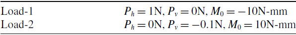
Table 5. Loading parameters for the corrugated structure with top skin
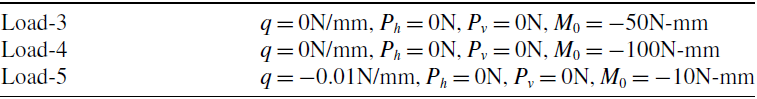
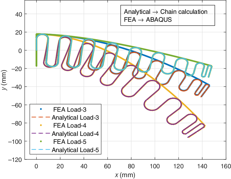
Figure 17. Deformed shapes of cantilever single corrugated structure with skin on top surface.
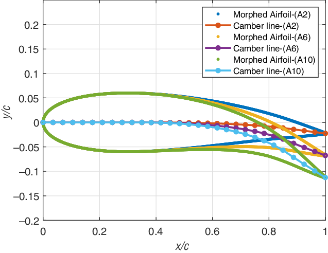
Figure 18. Deformed morphing aerofoil surfaces and camber lines for various morphing angles.

Figure 19. Drag polar for baseline aerofoil: validation of numerical methods.
3.2 Validation of numerical methods for aerodynamic calculations
The validation of the numerical methods and comparison of the different solvers allows for some conclusions to be drawn regarding the choice of tool for efficient computation. To compare the results from XFoil, Fluent and OpenFOAM simulations with experimental data [Reference Loftin and Smith38], the variation of the coefficient of drag ( $C_d$
) with respect to the coefficient of lift (
$C_d$
) with respect to the coefficient of lift ( $C_l$
), that is, the drag polar, is plotted for the baseline NACA0012 aerofoil in Fig. 19.
$C_l$
), that is, the drag polar, is plotted for the baseline NACA0012 aerofoil in Fig. 19.
From these plots, it can be observed that the estimation of $C_d$
by the two CFD solvers is roughly similar at lower values of
$C_d$
by the two CFD solvers is roughly similar at lower values of $C_l$
, that is, at lower angles of attack, while there is a noticeable disparity in
$C_l$
, that is, at lower angles of attack, while there is a noticeable disparity in $C_d$
at higher angles of attack. For instance, at a
$C_d$
at higher angles of attack. For instance, at a $C_l$
of nearly 0.2, the disparity in
$C_l$
of nearly 0.2, the disparity in $C_d$
is just 0.2%, whereas at a
$C_d$
is just 0.2%, whereas at a $C_l$
of nearly 1.0, the
$C_l$
of nearly 1.0, the $C_d$
prediction by OpenFOAM is almost 7% higher than that of Fluent. The XFoil simulations on the other hand consistently display lower
$C_d$
prediction by OpenFOAM is almost 7% higher than that of Fluent. The XFoil simulations on the other hand consistently display lower $C_d$
. This is because the XFoil simulations employ a transition model, which results in a laminar–turbulent boundary layer over the aerofoil and hence lower skin friction compared with a boundary layer that is turbulent over the entire aerofoil. As skin friction is expected to be dominant at low angles of attack, the drag predicted by XFoil is lower compared with the fully turbulent CFD simulations computed using OpenFOAM or Fluent. At lower
$C_d$
. This is because the XFoil simulations employ a transition model, which results in a laminar–turbulent boundary layer over the aerofoil and hence lower skin friction compared with a boundary layer that is turbulent over the entire aerofoil. As skin friction is expected to be dominant at low angles of attack, the drag predicted by XFoil is lower compared with the fully turbulent CFD simulations computed using OpenFOAM or Fluent. At lower $C_l$
, that is, 0
$C_l$
, that is, 0 $\leq$ $C_l$
$C_l$ $\leq$
0.6, the experimental data reported by Loftin and Smith [Reference Loftin and Smith38] are nearly similar to the drag predictions of XFoil. However, when
$\leq$
0.6, the experimental data reported by Loftin and Smith [Reference Loftin and Smith38] are nearly similar to the drag predictions of XFoil. However, when $C_l$
$C_l$ $>$
0.7, the experimental data deviate from the XFoil predictions and approach the values predicted by the CFD solvers. Comparisons could not be drawn beyond
$>$
0.7, the experimental data deviate from the XFoil predictions and approach the values predicted by the CFD solvers. Comparisons could not be drawn beyond $C_l$
$C_l$ $>$
1 due to the lack of experimental data in this region. Thus, it can be argued that, while drag predictions using XFoil are accurate at lower
$>$
1 due to the lack of experimental data in this region. Thus, it can be argued that, while drag predictions using XFoil are accurate at lower $\alpha$
(or more appropriately lower
$\alpha$
(or more appropriately lower $C_l$
), the actual drag at higher lift is expected to lie somewhere between the prediction obtained using a CFD solver (with a fully turbulent flow assumption) and that predicted by XFoil. To further investigate the differences in predicted aerodynamic coefficients across the different numerical methods,
$C_l$
), the actual drag at higher lift is expected to lie somewhere between the prediction obtained using a CFD solver (with a fully turbulent flow assumption) and that predicted by XFoil. To further investigate the differences in predicted aerodynamic coefficients across the different numerical methods, $C_p$
and
$C_p$
and $C_f$
plots are compared for three different angles of attack marked in Fig. 19 in Appendix A.
$C_f$
plots are compared for three different angles of attack marked in Fig. 19 in Appendix A.
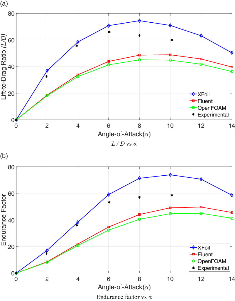
Figure 20. Variation of lift-to-drag ratio and endurance factor with angle-of-attack for baseline aerofoil.
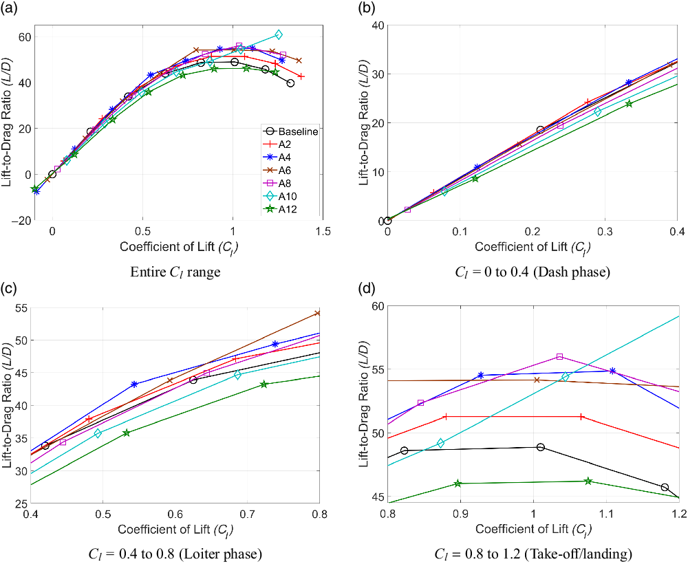
Figure 21. Coefficient of lift versus lift-to-drag ratio (Fluent) for SCVC aerofoils.

Figure 22. Coefficient of lift versus lift-to-drag ratio (XFoil) for SCVC aerofoils.
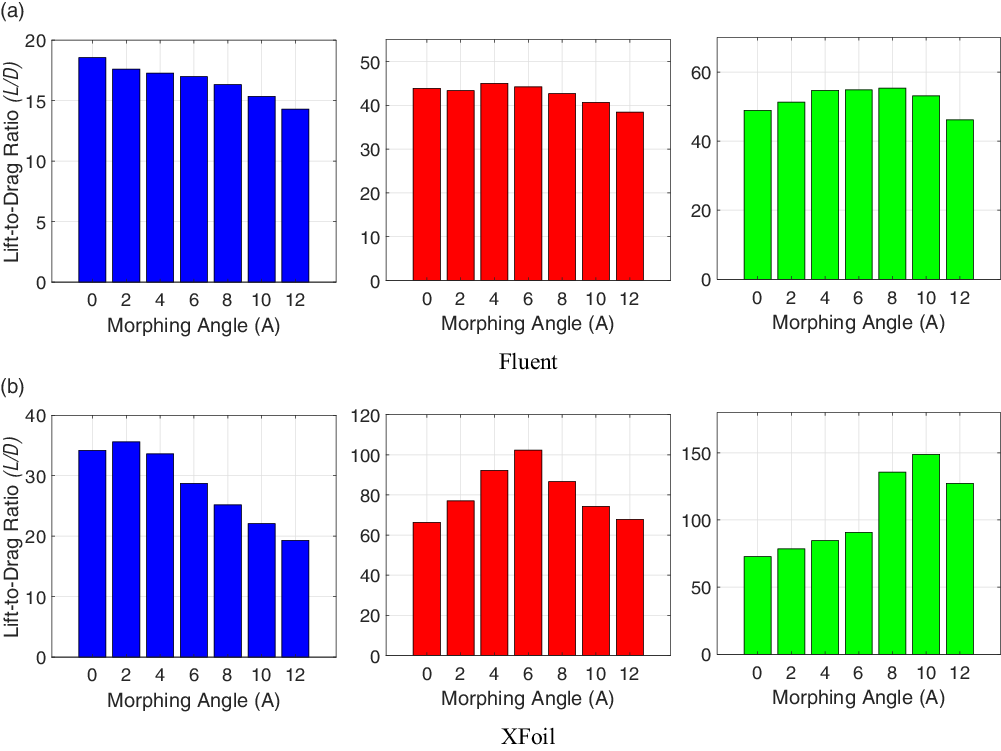
Figure 23. Lift-to-drag ratio versus morphing angle for $C_l$
= 0.2 (blue),
$C_l$
= 0.2 (blue), $C_l$
= 0.6 (red) and
$C_l$
= 0.6 (red) and $C_l$
= 1.0 (green).
$C_l$
= 1.0 (green).
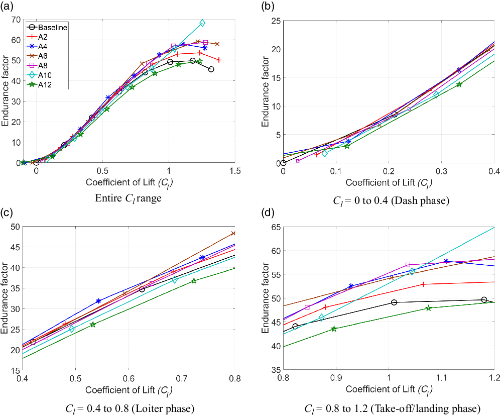
Figure 24. Coefficient of lift versus endurance factor (Fluent) for SCVC aerofoil.
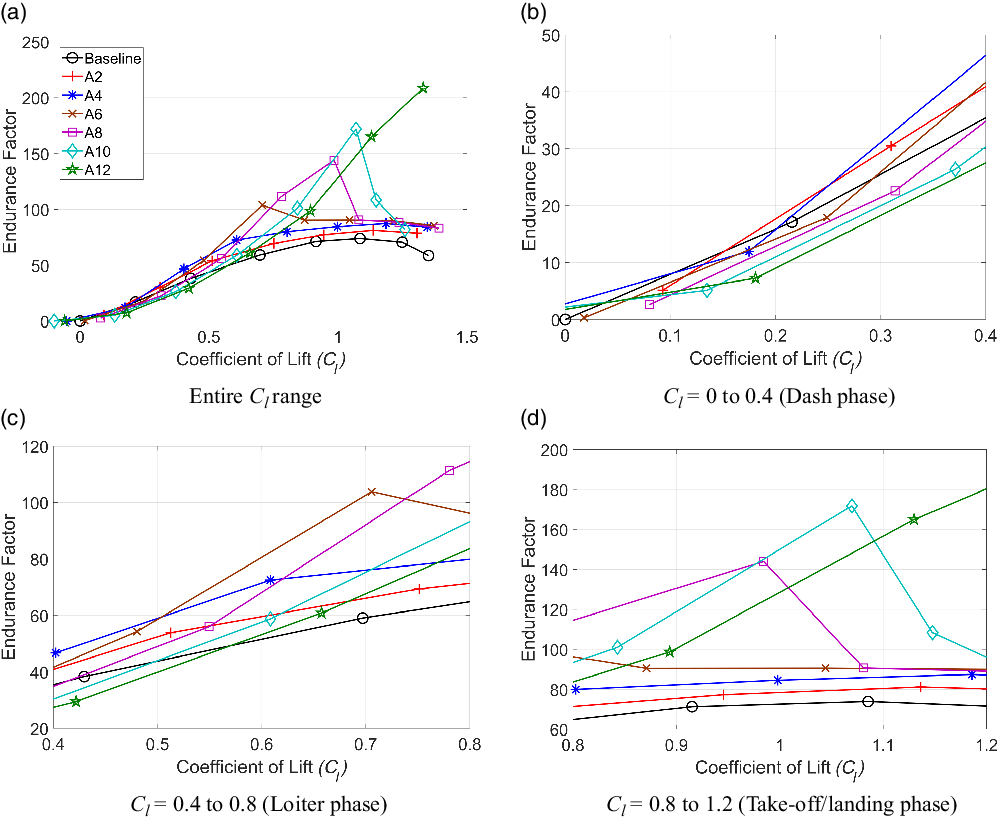
Figure 25. Coefficient of lift versus endurance factor (XFoil) for SCVC aerofoil.
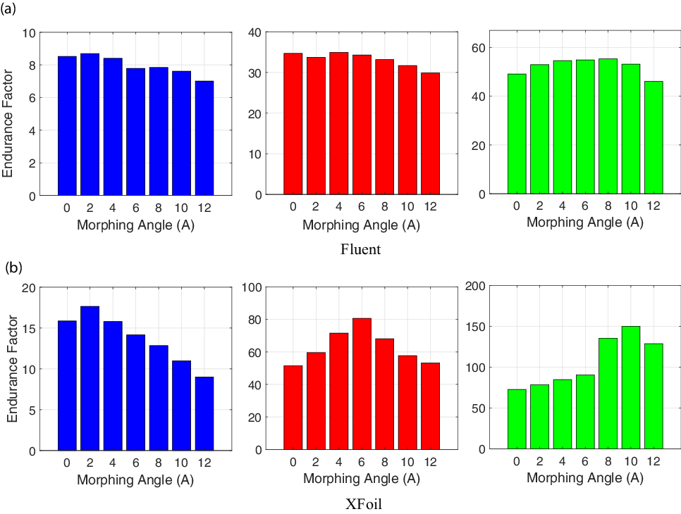
Figure 26. Endurance factor versus morphing angle for $C_l$
= 0.2 (blue),
$C_l$
= 0.2 (blue), $C_l$
= 0.6 (red) and
$C_l$
= 0.6 (red) and $C_l$
= 1.0 (green).
$C_l$
= 1.0 (green).
The variation of the lift-to-drag ratio ( $L/D$
) and endurance factor with the angle-of-attack (
$L/D$
) and endurance factor with the angle-of-attack ( $\alpha$
) is shown in Fig. 20(a) and (b). As can be seen from these figures, the
$\alpha$
) is shown in Fig. 20(a) and (b). As can be seen from these figures, the $L/D$
ratio and endurance factor estimated by the two CFD solvers are nearly identical until
$L/D$
ratio and endurance factor estimated by the two CFD solvers are nearly identical until $\alpha = 6^\circ$
. Beyond this
$\alpha = 6^\circ$
. Beyond this $\alpha$
, the disparity between the predictions of the two solver is more noticeable and grows with increase in
$\alpha$
, the disparity between the predictions of the two solver is more noticeable and grows with increase in $\alpha$
. The
$\alpha$
. The $L/D$
ratio and endurance factor predicted by XFoil are somewhat larger than the CFD estimations. This is due to the fact that the drag predicted by XFoil is lower than the fully turbulent CFD predictions, as observed in Fig. 19. The
$L/D$
ratio and endurance factor predicted by XFoil are somewhat larger than the CFD estimations. This is due to the fact that the drag predicted by XFoil is lower than the fully turbulent CFD predictions, as observed in Fig. 19. The $L/D$
ratio and endurance factor obtained from the experimental data are comparable to the XFoil predictions until
$L/D$
ratio and endurance factor obtained from the experimental data are comparable to the XFoil predictions until $\alpha = 6^\circ$
, after which the experimental data begin to deviate and tend to approach the CFD estimations. The largest
$\alpha = 6^\circ$
, after which the experimental data begin to deviate and tend to approach the CFD estimations. The largest $L/D$
ratios displayed by XFoil, Fluent and OpenFOAM predictions are 74.5 at
$L/D$
ratios displayed by XFoil, Fluent and OpenFOAM predictions are 74.5 at $\alpha$
=
$\alpha$
= $8^\circ$
, 48.9 at
$8^\circ$
, 48.9 at $\alpha = 10^\circ$
and 45 at
$\alpha = 10^\circ$
and 45 at $\alpha = 8^\circ$
, respectively. In the case of experimental data, the largest
$\alpha = 8^\circ$
, respectively. In the case of experimental data, the largest $L/D$
ratio of 66 is seen at
$L/D$
ratio of 66 is seen at $\alpha = 6^\circ$
. The peak endurance factors exhibited by the XFoil, Fluent and OpenFOAM predictions are 74 at
$\alpha = 6^\circ$
. The peak endurance factors exhibited by the XFoil, Fluent and OpenFOAM predictions are 74 at $\alpha = 10^\circ$
, 49.7 at
$\alpha = 10^\circ$
, 49.7 at $\alpha = 12^\circ$
and 45 at
$\alpha = 12^\circ$
and 45 at $\alpha = 12^\circ$
, respectively. The greatest endurance factor observed in the experimental data is 58.5 at an
$\alpha = 12^\circ$
, respectively. The greatest endurance factor observed in the experimental data is 58.5 at an $\alpha$
of nearly
$\alpha$
of nearly $10^\circ$
. It is also observed that the CFD predictions by Fluent compare better with experimental data than the OpenFOAM predictions.
$10^\circ$
. It is also observed that the CFD predictions by Fluent compare better with experimental data than the OpenFOAM predictions.
A point to note is that, although an attempt is made in this work to use the same solver options in OpenFOAM and Fluent, that is the same, higher-order extension (second-order upwind), incompressible solver (SIMPLE) and turbulence model (Menters SST), there are inadvertent differences present. For instance, the gradient reconstruction methods for the two solvers are not the same (Green–Gauss node based for Fluent but Gauss linear for OpenFOAM) as the same option is not available. Furthermore, the implementation of the turbulence model also has apparent differences (for instance, the way the eddy viscosity is defined) as listed in the Fluent [39] and OpenFOAM [40] manual pages. The aforementioned factors may play a role in the differences observed between the Fluent and OpenFOAM results. All subsequent CFD simulations presented in this work use Fluent.
3.3 Effect of morphing on aerodynamic characteristics
The aerodynamic performance of an aerofoil provides insight into the optimum aerofoil configuration in different flight phases. It can be quantitatively estimated by calculating the lift-to-drag ratio ( $L/D$
), which determines the maximum range of the aircraft, and the endurance factor
$L/D$
), which determines the maximum range of the aircraft, and the endurance factor $(C_l^{3/2}/C_d)$
, indicative of its propulsive power requirement and hence endurance. In this section, the variation of the
$(C_l^{3/2}/C_d)$
, indicative of its propulsive power requirement and hence endurance. In this section, the variation of the $L/D$
ratio and endurance factor with
$L/D$
ratio and endurance factor with $C_l$
is presented for both Fluent and XFoil simulations. Furthermore, the effect of morphing on these characteristics at a constant
$C_l$
is presented for both Fluent and XFoil simulations. Furthermore, the effect of morphing on these characteristics at a constant $C_l$
is also investigated.
$C_l$
is also investigated.
3.3.1 Lift-to-drag ratio (L/D)
To determine the effect of morphing on the aerodynamic performance, the $L/D$
ratio is plotted against
$L/D$
ratio is plotted against $C_l$
in Fig. 21. The aerodynamic coefficients in these figures are obtained from Fluent simulations. Figure 21(a) illustrates the variation of
$C_l$
in Fig. 21. The aerodynamic coefficients in these figures are obtained from Fluent simulations. Figure 21(a) illustrates the variation of $L/D$
for all the morphed cases over the entire range of
$L/D$
for all the morphed cases over the entire range of $C_l$
. The entire
$C_l$
. The entire $C_l$
range is further subdivided into three sub-ranges that roughly correspond to the three different flight phases, namely dash (Fig. 21(b)), loiter (Fig. 21(c)) and take-off/landing (Fig. 21(d)).
$C_l$
range is further subdivided into three sub-ranges that roughly correspond to the three different flight phases, namely dash (Fig. 21(b)), loiter (Fig. 21(c)) and take-off/landing (Fig. 21(d)).
In Fig. 21(b), which can be considered to represent the dash phase, it is seen that $L/D$
decrease with increase in the morphing angle. Clearly, non-morphed aerofoils and morphed aerofoils with small morphing angle (A2 and A4) perform better than aerofoils with medium morphing angles (A6 & A8) or large morphing angles (A10 & A12). In the loiter flight phase, as shown in Fig. 21(c), the effect of morphing is seen to have a positive effect on the
$L/D$
decrease with increase in the morphing angle. Clearly, non-morphed aerofoils and morphed aerofoils with small morphing angle (A2 and A4) perform better than aerofoils with medium morphing angles (A6 & A8) or large morphing angles (A10 & A12). In the loiter flight phase, as shown in Fig. 21(c), the effect of morphing is seen to have a positive effect on the $L/D$
ratio relative to the baseline aerofoil. Morphed aerofoils with small and medium morphing angles seem to outperform the baseline case and aerofoils with large morphing angles. Finally, for the highest
$L/D$
ratio relative to the baseline aerofoil. Morphed aerofoils with small and medium morphing angles seem to outperform the baseline case and aerofoils with large morphing angles. Finally, for the highest $C_l$
range (take-off/landing phase), as shown in Fig. 21(d), the
$C_l$
range (take-off/landing phase), as shown in Fig. 21(d), the $L/D$
for all the aerofoils except A10 seemed to have peaked. All the morphed cases with the exception of A12 outperform the baseline aerofoil.
$L/D$
for all the aerofoils except A10 seemed to have peaked. All the morphed cases with the exception of A12 outperform the baseline aerofoil.
The aerodynamic performance of the SCVC aerofoils as predicted by XFoil is shown in Fig. 22. As can be seen from Fig. 22(a), the range of $L/D$
is greater than observed in the Fluent simulations. This is expected as
$L/D$
is greater than observed in the Fluent simulations. This is expected as $C_d$
predicted by XFoil is relatively lower, whereas
$C_d$
predicted by XFoil is relatively lower, whereas $C_l$
values are close, compared with the Fluent simulations, which results in higher
$C_l$
values are close, compared with the Fluent simulations, which results in higher $L/D$
ratios compared with Fluent predictions. Distinct peaks in
$L/D$
ratios compared with Fluent predictions. Distinct peaks in $L/D$
are also observed for certain morphed configurations in the plot. It is seen that, in the dash phase as shown in Fig. 22(b), the baseline and aerofoils with lower degrees of morphing such as A2 and A4 display larger
$L/D$
are also observed for certain morphed configurations in the plot. It is seen that, in the dash phase as shown in Fig. 22(b), the baseline and aerofoils with lower degrees of morphing such as A2 and A4 display larger $L/D$
when compared with other morphed configurations. In the loiter flight phase as seen in Fig. 22(c), morphing is seen to have a largely positive effect on the aerodynamic performance. It can be seen that small and medium morphing angles exhibit significantly greater
$L/D$
when compared with other morphed configurations. In the loiter flight phase as seen in Fig. 22(c), morphing is seen to have a largely positive effect on the aerodynamic performance. It can be seen that small and medium morphing angles exhibit significantly greater $L/D$
when compared with large morphing angles as well as the baseline case. Finally, in the take-off/landing flight phase as shown in Fig. 22(d), all morphed aerofoils are seen to display greater
$L/D$
when compared with large morphing angles as well as the baseline case. Finally, in the take-off/landing flight phase as shown in Fig. 22(d), all morphed aerofoils are seen to display greater $L/D$
when compared with the baseline aerofoil throughout the entire flight phase. It can also be observed that aerofoils with large morphing angles are more favourable.
$L/D$
when compared with the baseline aerofoil throughout the entire flight phase. It can also be observed that aerofoils with large morphing angles are more favourable.
Figure 23 shows the variation of $L/D$
with morphing angle at
$L/D$
with morphing angle at $C_l$
= 0.2, 0.6 and 1.0. These
$C_l$
= 0.2, 0.6 and 1.0. These $C_l$
values serve as representative values for each of the three flight phases of dash, loiter and take-off/landing. The
$C_l$
values serve as representative values for each of the three flight phases of dash, loiter and take-off/landing. The $L/D$
for all the cases corresponding to the representative
$L/D$
for all the cases corresponding to the representative $C_l$
values are obtained through linear interpolation. The baseline case is represented by a morphing angle of
$C_l$
values are obtained through linear interpolation. The baseline case is represented by a morphing angle of $0^\circ$
. As seen from the Fluent results in Fig. 23(a), at
$0^\circ$
. As seen from the Fluent results in Fig. 23(a), at $C_l$
= 0.2, increasing the morphing angle decreases the aerodynamic performance. For instance, the
$C_l$
= 0.2, increasing the morphing angle decreases the aerodynamic performance. For instance, the $L/D$
at baseline is approximately 18.6 while that of A12 is 14.3. In the loiter phase at
$L/D$
at baseline is approximately 18.6 while that of A12 is 14.3. In the loiter phase at $C_l$
= 0.6, at a morphing angle of
$C_l$
= 0.6, at a morphing angle of $4^\circ$
, the
$4^\circ$
, the $L/D$
reaches a maximum of nearly 45 and any further increase in morphing angle reduces
$L/D$
reaches a maximum of nearly 45 and any further increase in morphing angle reduces $L/D$
. The largest morphing angle
$L/D$
. The largest morphing angle $12^\circ$
displays the lowest
$12^\circ$
displays the lowest $L/D$
of nearly 38.4. Finally at a
$L/D$
of nearly 38.4. Finally at a $C_l$
= 1.0, increasing the morphing angle results in increase of
$C_l$
= 1.0, increasing the morphing angle results in increase of $L/D$
until A8, where the
$L/D$
until A8, where the $L/D$
is 55.3. After this angle,
$L/D$
is 55.3. After this angle, $L/D$
drops, reaching a minimum of 46.1 at A12.
$L/D$
drops, reaching a minimum of 46.1 at A12.
Figure 23(b) shows the variation of $L/D$
with morphing angle as predicted by XFoil. In the dash phase, where
$L/D$
with morphing angle as predicted by XFoil. In the dash phase, where $C_l$
= 0.2, it is evident that A2 displays the largest
$C_l$
= 0.2, it is evident that A2 displays the largest $L/D$
of 35.6. Increasing the morphing angle further reduces
$L/D$
of 35.6. Increasing the morphing angle further reduces $L/D$
, with A12 exhibiting an
$L/D$
, with A12 exhibiting an $L/D$
of 19.3. At
$L/D$
of 19.3. At $C_l$
= 0.6,
$C_l$
= 0.6, $L/D$
increases with increasing morphing angle until
$L/D$
increases with increasing morphing angle until $6^\circ$
where
$6^\circ$
where $L/D$
is approximately 102.
$L/D$
is approximately 102. $L/D$
then starts to decrease with further increase in morphing angle. The baseline displays the lowest
$L/D$
then starts to decrease with further increase in morphing angle. The baseline displays the lowest $L/D$
of nearly 66 in this flight phase. Lastly at
$L/D$
of nearly 66 in this flight phase. Lastly at $C_l$
= 1.0, it is can be seen that increase in morphing angle is associated with increase in
$C_l$
= 1.0, it is can be seen that increase in morphing angle is associated with increase in $L/D$
until A10, where it reaches a maximum value of 149. After this morphing angle,
$L/D$
until A10, where it reaches a maximum value of 149. After this morphing angle, $L/D$
drops. The baseline aerofoil displays the lowest
$L/D$
drops. The baseline aerofoil displays the lowest $L/D$
of nearly 72.73.
$L/D$
of nearly 72.73.
From these observations, it can be stated that an optimum value of morphing exists for each flight stage, and that this value increases with the lift coefficient required. Thus, while a morphing angle of $2^\circ$
is best suited for the dash phase, the best morphing angle is
$2^\circ$
is best suited for the dash phase, the best morphing angle is $10^\circ$
for the take-off/landing.
$10^\circ$
for the take-off/landing.
3.3.2 Endurance factor
The variation of the endurance factor with $C_l$
from the Fluent simulations is plotted in Fig. 24. Similar to the
$C_l$
from the Fluent simulations is plotted in Fig. 24. Similar to the $L/D$
versus
$L/D$
versus $C_l$
plots, the
$C_l$
plots, the $C_l$
range is divided into three flight regimes, namely dash, loiter and take-off/landing. In the dash phase as seen in Fig. 24(b), morphed cases with small morphing angles exhibit marginally higher endurance in comparison with the baseline case. However, morphed cases with medium and large morphing angles exhibit lower endurance when compared with the baseline case. In the loiter phase as shown in Fig. 24(c), the effect of morphing is more pronounced. It can be seen that most morphing angles (small to medium) exhibit nearly similar or larger endurance relative to the baseline, while morphed cases with large morphing angles such as A10 and A12 are seen to display lower endurance. In the take-off/landing phase as seen in Fig. 24(d), morphing is seen to be most beneficial as almost all the morphing angles (with the exception of A12) display larger endurance relative to the baseline.
$C_l$
range is divided into three flight regimes, namely dash, loiter and take-off/landing. In the dash phase as seen in Fig. 24(b), morphed cases with small morphing angles exhibit marginally higher endurance in comparison with the baseline case. However, morphed cases with medium and large morphing angles exhibit lower endurance when compared with the baseline case. In the loiter phase as shown in Fig. 24(c), the effect of morphing is more pronounced. It can be seen that most morphing angles (small to medium) exhibit nearly similar or larger endurance relative to the baseline, while morphed cases with large morphing angles such as A10 and A12 are seen to display lower endurance. In the take-off/landing phase as seen in Fig. 24(d), morphing is seen to be most beneficial as almost all the morphing angles (with the exception of A12) display larger endurance relative to the baseline.
The variation of the endurance factor with $C_l$
as predicted by XFoil is shown in Fig. 25. The endurance factor predicted by XFoil is qualitatively similar to those predicted by Fluent across the different
$C_l$
as predicted by XFoil is shown in Fig. 25. The endurance factor predicted by XFoil is qualitatively similar to those predicted by Fluent across the different $C_l$
ranges, albeit larger in magnitude. In general, morphing results in better aerodynamic performance compared with the baseline aerofoil. Specifically, in the range of
$C_l$
ranges, albeit larger in magnitude. In general, morphing results in better aerodynamic performance compared with the baseline aerofoil. Specifically, in the range of $C_l$
identified with take-off/landing shown in Fig. 25(d), all the morphed cases display enhanced endurance relative to the baseline case throughout the entire phase.
$C_l$
identified with take-off/landing shown in Fig. 25(d), all the morphed cases display enhanced endurance relative to the baseline case throughout the entire phase.
Figure 27. $L/D$
ratio and endurance factor for fixed transition (at 5% chord) simulations in Xfoil:
$L/D$
ratio and endurance factor for fixed transition (at 5% chord) simulations in Xfoil: $C_l$
= 0.2 (blue),
$C_l$
= 0.2 (blue), $C_l$
= 0.6 (red) and
$C_l$
= 0.6 (red) and $C_l$
= 1.0 (green).
$C_l$
= 1.0 (green).
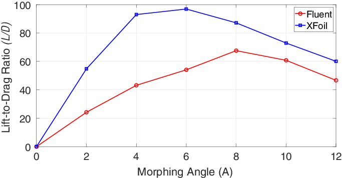
Figure 28. Variation of $L/D$
with morphing angle (A) at
$L/D$
with morphing angle (A) at $\alpha = 0^\circ$
.
$\alpha = 0^\circ$
.
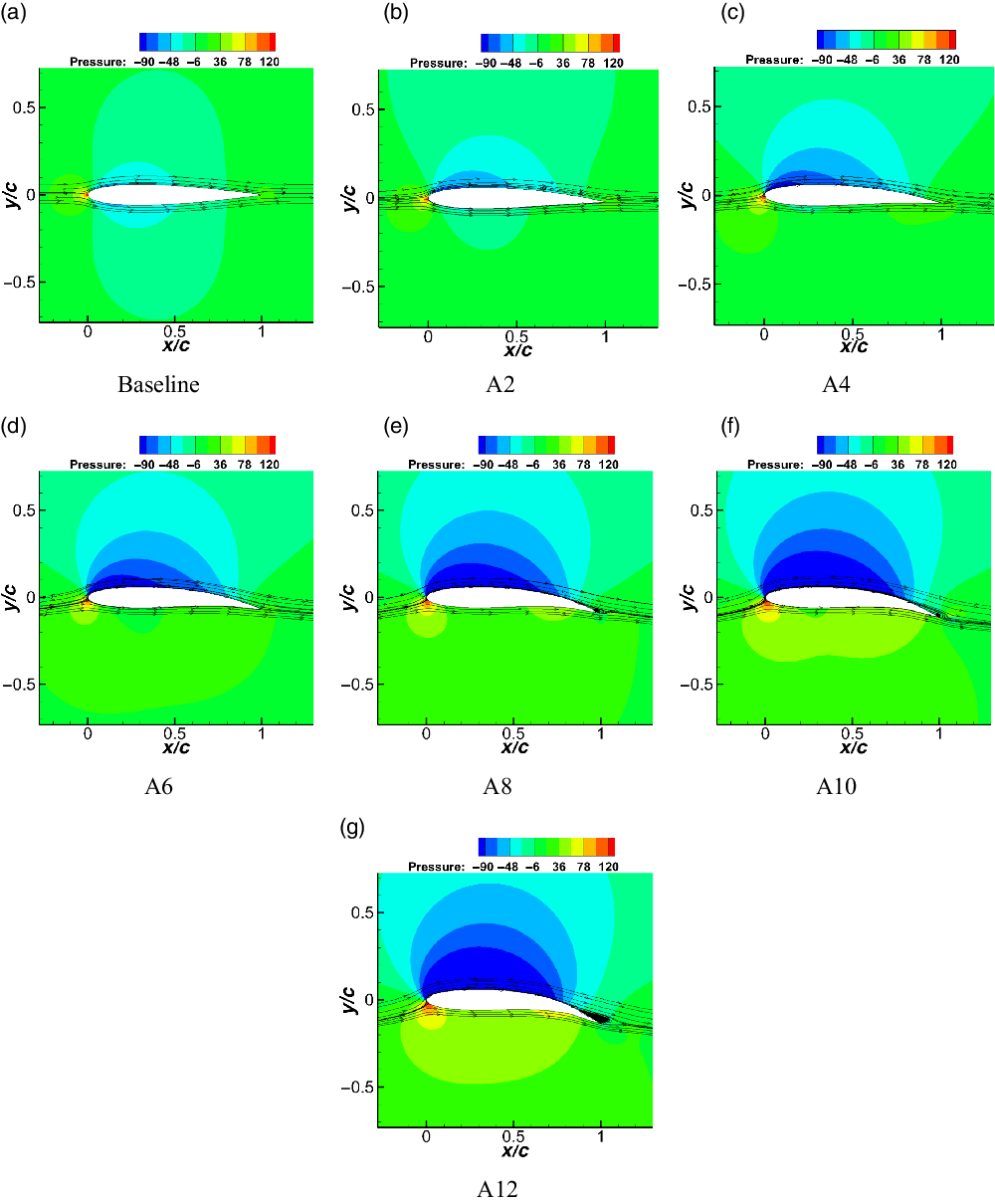
Figure 29. Pressure contours around different morphed aerofoils at $\alpha = 0^\circ$
.
$\alpha = 0^\circ$
.
The effect of morphing on the endurance factor at representative $C_l$
values of 0.2, 0.6 and 1.0 from the three flight phases as predicted by Fluent and XFoil is shown in Fig. 26. Similar to Fig. 23, the baseline aerofoil is represented by a morphing angle of
$C_l$
values of 0.2, 0.6 and 1.0 from the three flight phases as predicted by Fluent and XFoil is shown in Fig. 26. Similar to Fig. 23, the baseline aerofoil is represented by a morphing angle of $0^\circ$
. At a dash phase
$0^\circ$
. At a dash phase $C_l$
= 0.2, a marginal increase in endurance is observed when the baseline is morphed to
$C_l$
= 0.2, a marginal increase in endurance is observed when the baseline is morphed to $2^\circ$
, as seen in Fig. 26(a) from the Fluent predictions. Further increase in morphing angle is seen to decrease the endurance factor. Morphed aerofoil A2 displays the highest endurance of 8.7, while A12 displays the lowest endurance of 7. For
$2^\circ$
, as seen in Fig. 26(a) from the Fluent predictions. Further increase in morphing angle is seen to decrease the endurance factor. Morphed aerofoil A2 displays the highest endurance of 8.7, while A12 displays the lowest endurance of 7. For $C_l$
= 0.6, the endurance factor peaks to a value of nearly 35 at a morphing angle of
$C_l$
= 0.6, the endurance factor peaks to a value of nearly 35 at a morphing angle of $4^\circ$
. Further increase in morphing angle results in decrease of endurance factor, with A12 displaying the lowest endurance of nearly 29.9. Finally, at
$4^\circ$
. Further increase in morphing angle results in decrease of endurance factor, with A12 displaying the lowest endurance of nearly 29.9. Finally, at $C_l$
= 1.0, increasing the morphing angle increases the endurance factor until A8, where the endurance value is approximately 55.3. Subsequently, increasing the morphing angle reduces the endurance factor, with A12 exhibiting the least endurance factor of 46.
$C_l$
= 1.0, increasing the morphing angle increases the endurance factor until A8, where the endurance value is approximately 55.3. Subsequently, increasing the morphing angle reduces the endurance factor, with A12 exhibiting the least endurance factor of 46.
Figure 26(b) shows the variation of the endurance factor with morphing angle as predicted by XFoil. At $C_l$
= 0.2, morphing the baseline aerofoil to
$C_l$
= 0.2, morphing the baseline aerofoil to $2^\circ$
increases the endurance to a maximum value of nearly 17.7. Increasing the morphing angle further decreases the endurance factor. The aerofoil with the highest degree of morphing (A12) displays the lowest endurance factor of 9. In the loiter phase represented by a
$2^\circ$
increases the endurance to a maximum value of nearly 17.7. Increasing the morphing angle further decreases the endurance factor. The aerofoil with the highest degree of morphing (A12) displays the lowest endurance factor of 9. In the loiter phase represented by a $C_l$
= 0.6, the endurance increases with increase in morphing angle until it reaches a maximum value at a morphing angle of
$C_l$
= 0.6, the endurance increases with increase in morphing angle until it reaches a maximum value at a morphing angle of $6^\circ$
. The endurance then drops with further increase in morphing angle. Morphed aerofoil A6 shows a maximum endurance factor of 80.6, and the baseline aerofoil displays the lowest endurance of nearly 51.6. At
$6^\circ$
. The endurance then drops with further increase in morphing angle. Morphed aerofoil A6 shows a maximum endurance factor of 80.6, and the baseline aerofoil displays the lowest endurance of nearly 51.6. At $C_l$
= 1.0, the endurance increases with increase in the degree of morphing until a morphing angle of
$C_l$
= 1.0, the endurance increases with increase in the degree of morphing until a morphing angle of $10^\circ$
, where the value of endurance is nearly 150.1. Increasing the morphing angle further to
$10^\circ$
, where the value of endurance is nearly 150.1. Increasing the morphing angle further to $12^\circ$
decreases the endurance factor. The baseline case exhibits the lowest endurance factor of approximately 73. Evidently, these observations are similar to the conclusions drawn from Fig. 23. At lower
$12^\circ$
decreases the endurance factor. The baseline case exhibits the lowest endurance factor of approximately 73. Evidently, these observations are similar to the conclusions drawn from Fig. 23. At lower $C_l$
, that is, in the dash phase, morphing is predominantly detrimental. In the loiter phase, intermediate morphing angles seem to be more favourable than the rest. Finally, in the take-off/landing stage, larger morphing angles are desired.
$C_l$
, that is, in the dash phase, morphing is predominantly detrimental. In the loiter phase, intermediate morphing angles seem to be more favourable than the rest. Finally, in the take-off/landing stage, larger morphing angles are desired.
An important observation that can be made based on the results presented in Section 3.3 is that, as the desired $C_l$
increases, so does the optimal morphing angle. Further, this is primarily evident from the XFoil simulations but not from those obtained from Fluent. The possible reason that explains these observations is that the laminar-to-turbulent transition at a particular
$C_l$
increases, so does the optimal morphing angle. Further, this is primarily evident from the XFoil simulations but not from those obtained from Fluent. The possible reason that explains these observations is that the laminar-to-turbulent transition at a particular $C_l$
value shifts downstream as the morphing angle is increased, similar to what happens when cruise flaps are used [Reference McAvoy and Gopalarathnam41]. Thus, aerofoils with larger morphing have lower drag at the same lift, resulting in higher lift-to-drag ratio and endurance factor. Also, since Fluent simulations are run as fully turbulent, it cannot predict this trend. To validate this hypothesis, XFoil simulations are recomputed at a fixed transition location of low
$C_l$
value shifts downstream as the morphing angle is increased, similar to what happens when cruise flaps are used [Reference McAvoy and Gopalarathnam41]. Thus, aerofoils with larger morphing have lower drag at the same lift, resulting in higher lift-to-drag ratio and endurance factor. Also, since Fluent simulations are run as fully turbulent, it cannot predict this trend. To validate this hypothesis, XFoil simulations are recomputed at a fixed transition location of low $x/c$
(5% chord), and the aerodynamic parameters (
$x/c$
(5% chord), and the aerodynamic parameters ( $L/D$
and endurance factor) are plotted at fixed lift values and different morphing angles. This is shown in Fig. 27. The figure reveals that, when the transition location is fixed close to the leading edge, the aerodynamic parameters have similar values as predicted by the Fluent computations (Figs 23(a) and 26(a)), which do not account for flow transition, and neither show any clear benefit due to camber morphing, nor a clear shift in the optimal morphing angle as
$L/D$
and endurance factor) are plotted at fixed lift values and different morphing angles. This is shown in Fig. 27. The figure reveals that, when the transition location is fixed close to the leading edge, the aerodynamic parameters have similar values as predicted by the Fluent computations (Figs 23(a) and 26(a)), which do not account for flow transition, and neither show any clear benefit due to camber morphing, nor a clear shift in the optimal morphing angle as $C_l$
increases.
$C_l$
increases.
3.4 Optimal morphing at fixed $\alpha$

To investigate the effect of morphing at a particular angle-of-attack, the lift-to-drag ratio predicted by XFoil and Fluent is plotted against the morphing angle (A) for the SCVC aerofoil at $\alpha = 0^\circ$
in Fig. 28. The baseline aerofoil is indicated by a morphing angle of
$\alpha = 0^\circ$
in Fig. 28. The baseline aerofoil is indicated by a morphing angle of $0^\circ$
. It can be seen that both plots show the presence of an optimal morphing angle at which the
$0^\circ$
. It can be seen that both plots show the presence of an optimal morphing angle at which the $L/D$
ratio reaches a maximum. In the case of XFoil, the peak
$L/D$
ratio reaches a maximum. In the case of XFoil, the peak $L/D$
occurs at A6, whereas for the Fluent case, the peak is displaced to a larger morphing angle at A8. The
$L/D$
occurs at A6, whereas for the Fluent case, the peak is displaced to a larger morphing angle at A8. The $L/D$
in the Fluent cases are relatively lower than obtained using XFoil because the Fluent simulations are performed under fully turbulent flow condition over the aerofoil.
$L/D$
in the Fluent cases are relatively lower than obtained using XFoil because the Fluent simulations are performed under fully turbulent flow condition over the aerofoil.
To better understand the observations made in Fig. 28, the pressure contours (along with streamlines) for the baseline and morphed configurations at $\alpha$
=
$\alpha$
= $0^\circ$
from the Fluent simulations are shown in Fig. 29. As the morphing angle increases from zero (thus producing a cambered aerofoil), the suction pressure over the aerofoil also correspondingly decreases (larger negative
$0^\circ$
from the Fluent simulations are shown in Fig. 29. As the morphing angle increases from zero (thus producing a cambered aerofoil), the suction pressure over the aerofoil also correspondingly decreases (larger negative $C_p$
). This results in larger lift generation along with an increase in
$C_p$
). This results in larger lift generation along with an increase in $L/D$
. However, as morphing angle of A8 is reached (which provides the maximum
$L/D$
. However, as morphing angle of A8 is reached (which provides the maximum $L/D$
ratio in this case), a small re-circulation region begins to develop near the trailing edge of the aerofoil due to flow separation. Increasing the morphing angle moves the separation point further upstream, resulting in a larger re-circulation region. Due to this, the pressure drag also correspondingly increases, thereby reducing the
$L/D$
ratio in this case), a small re-circulation region begins to develop near the trailing edge of the aerofoil due to flow separation. Increasing the morphing angle moves the separation point further upstream, resulting in a larger re-circulation region. Due to this, the pressure drag also correspondingly increases, thereby reducing the $L/D$
ratio. Although the present discussion considers a particular choice of
$L/D$
ratio. Although the present discussion considers a particular choice of $\alpha$
, a similar trend is expected to exist for different
$\alpha$
, a similar trend is expected to exist for different $\alpha$
, wherein an optimal value of camber exists that gives the maximum
$\alpha$
, wherein an optimal value of camber exists that gives the maximum $L/D$
ratio.
$L/D$
ratio.
4.0 Conclusions
This work investigates the aerodynamic characteristics of an aerofoil morphed using the single corrugated variable-camber concept. The following points are observed from this study:
-
Small-deformation analysis of the SCVC morphing wing is investigated using a beam model which is based on chain calculations. The deflected profiles obtained from this proposed model are verified and compared with ABAQUS®. The results from both methods agree well.
-
Aerodynamic coefficients are estimated using two different CFD solvers and XFoil. Both Fluent and OpenFOAM predict nearly similar results, while the XFoil simulations predict relatively lower drag as it employs a transition model. Further, it is also observed through comparison with experimental data that, while lift/drag predictions using XFoil are accurate at lower lift values, the actual lift/drag at moderate and higher lift values is expected to lie somewhere between the predictions obtained using a CFD solver (with fully turbulent flow assumption) and XFoil.
-
In the dash flight phase, characterised by a requirement for low
$C_l$
, the non-morphed baseline aerofoil performs better than morphed aerofoils. In the other flight phases, that is, loiter and take-off/landing, wherein the
$C_l$
requirement becomes progressively higher, the morphed aerofoils exhibit superior performance with respect to the baseline aerofoil. It is also observed that the maximum values of both the lift-to-drag ratio and endurance factor increase with morphing. These effects are primarily captured by the XFoil results but not in the Fluent simulations. The reason for this shift in the aerofoil optimal performance at larger morphing angles to higher
$C_l$
values is attributed to the downstream shift of transition (at fixed
$C_l$
) on the aerofoil surface as the morphing increases. This is verified by calculating the lift-to-drag ratio and endurance factor in XFoil for fixed transition near the leading edge (5% of chord) at representative
$C_l$
values (0.2, 0.6 and 1.0). The results obtained in this case are similar to those predicted by Fluent, which does not take flow transition into account. This indicates that benefits of camber morphing can only be (clearly) predicted by flow solver(s) that account for flow transition, as the change in the transition location with morphing plays an important role in this case. -
It is illustrated through the choice of a particular
$\alpha$
(=
$0^\circ$
) that there potentially exists a morphing angle for which the
$L/D$
ratio becomes a maximum for any
$\alpha$
. This is expected to happen, as flow separation can occur at higher morphing angles, which can offset the gain in lift achieved through camber morphing through an increase in pressure drag.


Acknowledgements
The work presented here was funded by grants from the Defense Research and Development Organization with sanction no. DRDO/DFTM/04/3304/PC/02/776/D(R $\&$
D).
$\&$
D).
APPENDIX
A Pressure and skin friction comparison among XFoil, Fluent and Open FOAM
The pressure distribution around the baseline aerofoil computed by XFoil and the two CFD solvers at three different angles of attack highlighted in Fig. 19 is shown in Fig. A.1. As seen in Fig. A.1(a), at $\alpha = 2^\circ$
, the coefficient of pressure (
$\alpha = 2^\circ$
, the coefficient of pressure ( $C_p$
) distributions over the surface of the aerofoil are nearly overlapping for the two CFD solvers. The
$C_p$
) distributions over the surface of the aerofoil are nearly overlapping for the two CFD solvers. The $C_p$
distribution for XFoil, however, is marginally different from the
$C_p$
distribution for XFoil, however, is marginally different from the $C_p$
distribution of the CFD solvers. On the suction side of the aerofoil, the pressure is slightly lower than that of the CFD solvers until
$C_p$
distribution of the CFD solvers. On the suction side of the aerofoil, the pressure is slightly lower than that of the CFD solvers until $x/c = 0.47$
. At this point, the pressure suddenly rises, indicating that the flow has transitioned from laminar to turbulent. Past the transition point, the suction pressure predicted by XFoil is nearly similar to the pressure predicted by the CFD solvers. On the pressure side of the aerofoil, the
$x/c = 0.47$
. At this point, the pressure suddenly rises, indicating that the flow has transitioned from laminar to turbulent. Past the transition point, the suction pressure predicted by XFoil is nearly similar to the pressure predicted by the CFD solvers. On the pressure side of the aerofoil, the $C_p$
is nearly identical for the two CFD solvers and XFoil, with the exception of the point
$C_p$
is nearly identical for the two CFD solvers and XFoil, with the exception of the point $x/c = 0.86$
where the pressure rises slightly, indicating the point of transition on the bottom side of the aerofoil. For the case
$x/c = 0.86$
where the pressure rises slightly, indicating the point of transition on the bottom side of the aerofoil. For the case $\alpha = 6^\circ$
as shown in Fig. A.1(b), similar to the previous case, the pressure distributions predicted by the two CFD solvers are nearly coincident. On the other hand, the pressure distribution predicted by XFoil is noticeably different in the region 0
$\alpha = 6^\circ$
as shown in Fig. A.1(b), similar to the previous case, the pressure distributions predicted by the two CFD solvers are nearly coincident. On the other hand, the pressure distribution predicted by XFoil is noticeably different in the region 0 $\leq \textrm{x}/\textrm{c} \leq 0.1$
as compared with the CFD solvers. The XFoil prediction exhibits a relatively higher peak negative pressure over the aerofoil. The transition on the top surface occurs at around
$\leq \textrm{x}/\textrm{c} \leq 0.1$
as compared with the CFD solvers. The XFoil prediction exhibits a relatively higher peak negative pressure over the aerofoil. The transition on the top surface occurs at around $x/c = 0.08$
. After the transition point, the
$x/c = 0.08$
. After the transition point, the $C_p$
distribution of XFoil is marginally lower than that of the two CFD solvers. The
$C_p$
distribution of XFoil is marginally lower than that of the two CFD solvers. The $C_p$
distribution on the bottom side is virtually similar for the CFD solvers and XFoil. Transition on the bottom side is not seen for this case. At
$C_p$
distribution on the bottom side is virtually similar for the CFD solvers and XFoil. Transition on the bottom side is not seen for this case. At $\alpha = 10^\circ$
as shown in Fig. A.1(c), the
$\alpha = 10^\circ$
as shown in Fig. A.1(c), the $C_p$
distribution trend among the CFD solvers and XFoil is similar to that of the other cases. The transition point on the top side occurs further upstream at
$C_p$
distribution trend among the CFD solvers and XFoil is similar to that of the other cases. The transition point on the top side occurs further upstream at $x/c = 0.024$
, while the transition point on the bottom side is not seen. The disparity in
$x/c = 0.024$
, while the transition point on the bottom side is not seen. The disparity in $C_l$
(higher for XFoil) observed at these
$C_l$
(higher for XFoil) observed at these $\alpha$
in Fig. 19 can be correlated to the difference in
$\alpha$
in Fig. 19 can be correlated to the difference in $C_p$
distribution of the XFoil and CFD solvers.
$C_p$
distribution of the XFoil and CFD solvers.

Figure A.1. $C_p$
distribution on baseline aerofoil.
$C_p$
distribution on baseline aerofoil.
To compare the skin friction drag predicted by the CFD solvers and XFoil, the distribution of coefficient of skin friction ( $C_f$
) is plotted for three different angles of attack, namely
$C_f$
) is plotted for three different angles of attack, namely $\alpha = 2^\circ$
,
$\alpha = 2^\circ$
, $6^\circ$
and
$6^\circ$
and $10^\circ$
, in Fig. A.2. As can be seen from this figure, the
$10^\circ$
, in Fig. A.2. As can be seen from this figure, the $C_f$
distribution is nearly coincident for both CFD solvers for all three cases of
$C_f$
distribution is nearly coincident for both CFD solvers for all three cases of $\alpha$
. The
$\alpha$
. The $C_f$
distribution from XFoil, however, follows a different trend. This variation in
$C_f$
distribution from XFoil, however, follows a different trend. This variation in $C_f$
distribution occurs due to the fact that flow transition is accounted for in XFoil. For instance, the
$C_f$
distribution occurs due to the fact that flow transition is accounted for in XFoil. For instance, the $C_f$
values experience a sudden increase at
$C_f$
values experience a sudden increase at $x/c = 0.47$
for
$x/c = 0.47$
for $\alpha = 2^\circ$
on the top surface of the aerofoil, while on the bottom surface it occurs at
$\alpha = 2^\circ$
on the top surface of the aerofoil, while on the bottom surface it occurs at $x/c = 0.96$
, indicating flow transition. Similar transition points can be observed on the top surface of the aerofoil at
$x/c = 0.96$
, indicating flow transition. Similar transition points can be observed on the top surface of the aerofoil at $x/c = 0.08$
for
$x/c = 0.08$
for $\alpha = 6^\circ$
and
$\alpha = 6^\circ$
and $x/c = 0.024$
for
$x/c = 0.024$
for $\alpha = 10^\circ$
. These points also correspond to the transition locations (which show a sudden jump in pressure) observed in Fig. A.1. The
$\alpha = 10^\circ$
. These points also correspond to the transition locations (which show a sudden jump in pressure) observed in Fig. A.1. The $C_f$
predicted by XFoil is lower than that predicted by the CFD solvers upstream of the transition point. This explains the lower
$C_f$
predicted by XFoil is lower than that predicted by the CFD solvers upstream of the transition point. This explains the lower $C_d$
predicted by XFoil in Fig. 19.
$C_d$
predicted by XFoil in Fig. 19.
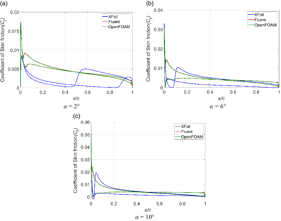
Figure A.2. $C_f$
distribution on baseline aerofoil.
$C_f$
distribution on baseline aerofoil.


 Open access