


Introduction
A prediction of the permanent income hypothesis is that households use savings in the event of an income shock to smooth consumption over their lifetimes. However, when households are lacking assets, it is likely that they have insufficient savings and face credit constraints, which render consumption smoothing almost impractical (Jappelli and Pistaferri Reference Jappelli and Pistaferri2010; Hallegatte et al. Reference Hallegatte, Vogt-Schilb, Bangalore and Rozenberg2017). It becomes obvious that an income shock to a low-asset household would imply a reduction in consumption expenses. Whether a reduction in expenses is concentrated in one consumption category or multiple categories is an important and relevant question for household well-being after income shocks.
The objective of this study is twofold: first, to determine how farm households adjust consumption expenses after an unexpected income loss due to natural disasters, and second, to evaluate whether an income loss experience affects producers' risk-taking behavior. We further complement the analysis with a survey of producers' resilience capacity against natural disasters. We focus specifically on specialty crop farm households in the Midwestern state of Indiana. This is due to the fact that (i) specialty crops in the Midwestern region are vulnerable to natural disasters, (ii) specialty crops' acres are the least covered by federal crop insurance, and (iii) Indiana specialty crop enterprises are mainly small in size and rely on family labor. In our results, we find that farm households reduce their monthly expenditures of food and miscellaneous categories by ~$119 and ~$280, respectively, after an income loss of 20–32 percent.Footnote 1 We also find that producers are less willing to take financial risk after an income loss experience.
Our study contributes to the literature on agricultural vulnerability to climate change and weather shocks (Walthall et al. Reference Walthall, Hatfield, Backlund, Lengnick, Marshall, Walsh, Adkins, Aillery, Ainsworth, Ammann, Anderson, Bartomeus, Baumgard, Booker, Bradley, Blumenthal, Bunce, Burkey, Dabney, Delgado, Dukes, Funk, Garrett, Glenn, Grantz, Goodrich, Hu, Izaurralde, Jones, Kim, Leaky, Lewers, Mader, McClung, Morgan, Muth, Nearing, Oosterhuis, Ort, Parmesan, Pettigrew, Polley, Rader, Rice, Rivington, Rosskopf, Salas, Sollenberger, Srygley, Stöckle, Takle, Timlin, White, Winfree, Wright-Morton and Ziska2013; Kistner et al. Reference Kistner, Kellner, Andresen, Todey and Morton2018; Grabrucker and Grimm Reference Grabrucker and Grimm2020). We estimate the potential impact of income loss due to natural disasters on Indiana specialty producers' household consumption expenses. Furthermore, our study contributes to the literature on producers' risk preferences in two areas: (i) We measure producers' risk preferences immediately after they experience natural disasters because it is an important time in terms of farm investment and household consumption decisions and (ii) we assess whether producers who receive a hypothetical negative income shock are more risk-averse than a counterfactual group of producers. These contributions relate to the literature on decreasing absolute risk aversion (Pratt Reference Pratt1964; Arrow Reference Arrow1971) and the nonstability of risk preferences over time (Malmendier and Nagel Reference Malmendier and Nagel2011; Guiso, Sapienza, and Zingales Reference Guiso, Sapienza and Zingales2018).
Specialty crops' production in the Midwestern United States was worth $5.24 billion in market value in 2017 (National Agricultural Statistics Service 2019c).Footnote 2 These crops' yields are subject to weather and climate threats, which are projected to be intensified by wetter springs and drier summers in the future (Kistner et al. Reference Kistner, Kellner, Andresen, Todey and Morton2018). It is already the case that U.S. agricultural losses are primarily driven by weather and climate disasters, that is, floods, droughts, and severe freezes (Smith Reference Smith2018). How well do producer households recover from a disaster depends on the recovery tools and mechanisms in place. Despite federal crop insurance being an important risk management tool for U.S. agricultural producers, specialty crops are among the least covered agricultural crops. Nationally, only 34 percent of eligible vegetable crops' acreage was enrolled in federal crop insurance programs in 2015 as compared to 89 percent of major crops, that is, corn, wheat, and soybean (Shields Reference Shields2017). In the case of fruits and nuts, 74 percent of the acreage was insured, which is still much lower than that of major crops (Shields Reference Shields2017). Moreover, the average total loss deductible for vegetables (35 percent) and fruits and nuts (41 percent) is higher than that for major crops (26 percent) (Shields Reference Shields2017).Footnote 3 Meanwhile, 86 percent of Indiana vegetable farms are classified as small and medium (less than $10,000 and $250,000 gross annual sales, respectively), and these farms mainly rely on family labor (Torres and Marshall Reference Torres and Marshall2016). Although farming is the primary occupation of around 41 percent of Indiana specialty producers (National Agricultural Statistics Service 2019a), the agricultural and asset losses from natural disasters can still have a deleterious effect on every farm household's income.
The consumption of low-income households is relatively more vulnerable to the negative effects of natural disasters than that of high-income households because low-income households often lack the assets to protect them against natural disasters (Hallegatte et al. Reference Hallegatte, Vogt-Schilb, Bangalore and Rozenberg2017). When a low-income household's consumption falls across food, health, and education categories, the household suffers a loss in well-being (Hallegatte et al. Reference Hallegatte, Vogt-Schilb, Bangalore and Rozenberg2017). For instance, a consumption decline across food, health, and education categories can translate into poor health for household members or low employment prospects for their children in the future.
Given that farm producers' insurance, marketing, and commodity supply decisions partially depend on their risk-taking capacity (Chavas and Holt Reference Chavas and Holt1996; Eckman, Patrick, and Musser Reference Eckman, Patrick and Musser1996; Zhao and Yue Reference Zhao and Yue2020), we investigate producers' risk preferences after a natural disaster and income loss experience. Understanding producers' consumption and risk behavior after a disaster can help with policies related to household recovery and designing credit and insurance instruments that can lessen the negative effects of natural disasters.
The study of consumption response and risk behavior after transitory income shocks is an active research area, although mired with data limitations (Attanasio and Weber Reference Attanasio and Weber2010; Christelis et al. Reference Christelis, Georgarakos, Jappelli, Pistaferri and van Rooij2019). A natural disaster, or any income shock, happens at irregular intervals, while survey collections mostly happen at regular intervals, so aligning them together becomes difficult, particularly if interest is in measuring consumption and risk before and after a shock. To the best of our knowledge, we are the first to study farm household consumption responses to exogenous income shocks, where identification is clearly obtained by using an experimental design, albeit through a hypothetical survey. Our methods can be easily extended to other contexts to study producers' household and farm decisions.
Literature Review
Agricultural production activity is mired with risk due to price and production volatility, policies, institutional arrangements, and weather (Hardaker et al. Reference Hardaker, Huirne, Anderson and Lien2004, pp. 1–4). In the case of rare “catastrophic” risks posed by natural weather events, producers lose crop production, which can directly affect their farm finances (Ogurtsov, Asseldonk, and Huirne Reference Ogurtsov, Asseldonk and Huirne2008). Agricultural risk can affect farm output and finances, hence the reason that U.S. agricultural policy allocates considerable resources to farm risk management. In what follows, we discuss research related to agricultural losses due to natural disasters and their potential economic impacts. Next, we discuss the literature on farmers' and nonfarmers' risk preferences, which are sometimes measured in the aftermath of natural disasters.
Too little or too much of precipitation, compounded with erratic temperatures, can bring about drought, floods, and severe freezes. Such natural disasters pose substantial and perpetual threats to agricultural production. In the U.S., droughts inflicted $15 billion in crop losses in 1988–1989 (Reibsame, Changnon, and Karl Reference Reibsame, Changnon and Karl1991), reduced corn and soybean yields by 0.1 percent to 1.2 percent per additional drought-week in 2001–2013 (Kuwayama et al. Reference Kuwayama, Thompson, Bernknopf, Zaitchik and Vail2019), and inflicted losses of $2 billion (crops) and $553 million (dairy and livestock) in California in 2014–2016 (Howitt et al. Reference Howitt, Medellín-Azuara, MacEwan, Lund and Sumner2014, Reference Howitt, Medellín-Azuara, MacEwan, Lund and Sumner2015; Medellín-Azuara et al. Reference Medellín-Azuara, MacEwan, Howitt, Sumner and Lund2016). The 1993 flooding in the Central United States caused $5 billion in crop losses (Shannon and Motha Reference Shannon and Motha2015). In 2019, the flooding in Nebraska led to $440 million in crop losses (Di Liberto Reference Di Liberto2019). Damaging freezes, which are common to the U.S. and Canada, have historically led to orange and citrus production losses in California and Florida; and crop and fruit damage in the Plains, the South, and the Midwest in 2007 (Shannon and Motha Reference Shannon and Motha2015). In 2020, the COVID-19 pandemic (if considered a natural disaster) severely affected the U.S. agricultural sector; it is estimated that the net farm income will decrease by about $20 billion (Westhoff et al. Reference Westhoff, Meyer, Binfield and Gerlt2020). The derecho of August 10, 2020, wreaked havoc on crops in Iowa and the U.S. Midwest—the estimated losses are projected to be about $4 billion, thus making the 2020 derecho one of the costliest weather events of the past decade (Voiland Reference Voiland2020).
Although natural disasters are a threat to agricultural production, they have pushed U.S. farmers to adapt and consider new methods and strategies, for instance, the use of climate data in farm decision-making, participation in crop insurance programs, crop diversification, soil conservation, and livestock breed selection (Walthall et al. Reference Walthall, Hatfield, Backlund, Lengnick, Marshall, Walsh, Adkins, Aillery, Ainsworth, Ammann, Anderson, Bartomeus, Baumgard, Booker, Bradley, Blumenthal, Bunce, Burkey, Dabney, Delgado, Dukes, Funk, Garrett, Glenn, Grantz, Goodrich, Hu, Izaurralde, Jones, Kim, Leaky, Lewers, Mader, McClung, Morgan, Muth, Nearing, Oosterhuis, Ort, Parmesan, Pettigrew, Polley, Rader, Rice, Rivington, Rosskopf, Salas, Sollenberger, Srygley, Stöckle, Takle, Timlin, White, Winfree, Wright-Morton and Ziska2013). Adaptive strategies may protect farm production if there is climatic stability; however, the twenty-first century is predicted to have more variable climatic conditions (Walthall et al. Reference Walthall, Hatfield, Backlund, Lengnick, Marshall, Walsh, Adkins, Aillery, Ainsworth, Ammann, Anderson, Bartomeus, Baumgard, Booker, Bradley, Blumenthal, Bunce, Burkey, Dabney, Delgado, Dukes, Funk, Garrett, Glenn, Grantz, Goodrich, Hu, Izaurralde, Jones, Kim, Leaky, Lewers, Mader, McClung, Morgan, Muth, Nearing, Oosterhuis, Ort, Parmesan, Pettigrew, Polley, Rader, Rice, Rivington, Rosskopf, Salas, Sollenberger, Srygley, Stöckle, Takle, Timlin, White, Winfree, Wright-Morton and Ziska2013). Erratic weather and climate are specifically harmful to specialty crops, which are more sensitive to climatic stressors than row crops (Kistner et al. Reference Kistner, Kellner, Andresen, Todey and Morton2018). From 1989 to 2015, specialty crops in the Midwest have been constantly affected by weather hazards (Kistner et al. Reference Kistner, Kellner, Andresen, Todey and Morton2018). In 2007, California lost about 20 percent of orange production due to severe freeze (Shannon and Motha Reference Shannon and Motha2015).
Given that natural disasters affect specialty crops' production, the low insurance coverage of these crops poses a financial risk to specialty crop farms. Despite the availability of the Non-Insurance Assistance Program (NAP) under the Federal Crop Insurance Reform Act of 1994, research shows that specialty producers were not compensated well enough compared with ad hoc disaster payments in 1988–1993 (Lee, Harwood, and Somwaru Reference Lee, Harwood and Somwaru1997). The Whole Farm Revenue Protection (WFRP) insurance serves as an attractive risk management option for specialty crop producers due to its higher premium subsidy rates than other insurance policies; however, participation rates for WFRP remain low (for instance, 0.1 percent of all insurance policies in Indiana are WFRP) (Olen and Wu Reference Olen and Wu2017). The gist of the above literature points toward the increasing vulnerability of farms and farmer livelihoods to climate change, more so true for small family farms (Walthall et al. Reference Walthall, Hatfield, Backlund, Lengnick, Marshall, Walsh, Adkins, Aillery, Ainsworth, Ammann, Anderson, Bartomeus, Baumgard, Booker, Bradley, Blumenthal, Bunce, Burkey, Dabney, Delgado, Dukes, Funk, Garrett, Glenn, Grantz, Goodrich, Hu, Izaurralde, Jones, Kim, Leaky, Lewers, Mader, McClung, Morgan, Muth, Nearing, Oosterhuis, Ort, Parmesan, Pettigrew, Polley, Rader, Rice, Rivington, Rosskopf, Salas, Sollenberger, Srygley, Stöckle, Takle, Timlin, White, Winfree, Wright-Morton and Ziska2013).
The impact of natural disasters on farmers' income and consumption is well documented for developing countries, where farming is small scale, and livelihoods depend on agricultural production. For instance, natural disasters' effects have been studied for consumption (Townsend Reference Townsend1994; Morduch Reference Morduch1995; Kazianga and Udry Reference Kazianga and Udry2006; Porter Reference Porter2012), farm and livestock management (Rosenzweig and Binswanger Reference Rosenzweig and Binswanger1993; Hoddinott Reference Hoddinott2006), and nutrition and health (Hoddinott Reference Hoddinott2006; Kazianga and Udry Reference Kazianga and Udry2006). Results from a recent study on the effects of rainfall shocks in rural Thailand suggest that (i) the impact of weather-based agricultural shocks is larger than what the current literature suggests and (ii) agricultural shocks affect input availability and costs for farm and nonfarm enterprises, and consumption expenditures for farm households (Grabrucker and Grimm Reference Grabrucker and Grimm2020). Our study contributes to the above strand of literature by estimating the potential impact of income loss due to natural disasters on Indiana specialty producers' consumption expenditures.
Given that farmers make decisions in risky environments, it is also important to understand their risk preferences, which affect business decisions regarding crop insurance, marketing, and commodity supply (Chavas and Holt Reference Chavas and Holt1996; Eckman, Patrick, and Musser Reference Eckman, Patrick and Musser1996; Zhao and Yue Reference Zhao and Yue2020). Following are the two key findings in the literature on farmers' risk preferences: (i) farmers' risk preferences are not the same across studies; on average, farmers are risk-averse, and (ii) from a methodological perspective, farmers should be able to comprehend the risk elicitation task, which can be improved with a contextualized presentation of the elicitation task (Iyer et al. Reference Iyer, Bozzola, Hirsch, Meraner and Finger2020). In terms of methodological developments in measuring farmers' risk preferences, the multi-item 5-point scales and lottery-based choice tasks are the most widely used methods since 2010, especially in European studies (Iyer et al. Reference Iyer, Bozzola, Hirsch, Meraner and Finger2020).
While there is a large economics literature on measuring risk preferences (see Starmer Reference Starmer2000; DellaVigna Reference DellaVigna2009; Barseghyan et al. Reference Barseghyan, Molinari, O'Donoghue and Teitelbaum2018), there is comparatively less on exploring how risk preferences might respond to exogenous income shocks or catastrophic disasters. In this regard, Chuang and Schechter (Reference Chuang and Schechter2015) provide a literature review of risk preferences after natural disasters, where some studies find an increase in risk aversion after disasters (Cameron and Shah Reference Cameron and Shah2015), others find a reduction in risk aversion (Eckel, El-Gamal, and Wilson Reference Eckel, El-Gamal and Wilson2009), and some find no change in risk aversion (Becchetti, Castriota, and Conzo Reference Becchetti, Castriota and Conzo2012). The diverging results on risk preferences after natural disasters are probably due to subtleties intrinsic to natural disasters, or it is possible that the experimental method in each study is contributing to the different results across studies (Chuang and Schechter Reference Chuang and Schechter2015). By measuring producers' risk preferences immediately after they experience a hypothetical natural disaster, our study aims to contribute to the diverse findings on disasters' effect on risk preferences (Chuang and Schechter Reference Chuang and Schechter2015).
Conceptual Framework
The decision-making units in our study are farm households. We are interested in investigating the effect of an unexpected income loss due to natural disasters on farm household consumption categories.
Chetty and Szeidl (Reference Chetty and Szeidl2007) provide the theoretical framework and initial evidence that when income shocks are “small” (income loss of up to 33 percent), households make downward adjustment in the consumption expenditures of “adjustable” goods like food rather than “commitment” goods such as durables, which have adjustment costs associated with them. The authors show that less than 33 percent of U.S. households cut the expenditures of durables like apparel and furniture; however, about 42 percent and 49 percent of U.S households cut the expenditures of adjustable goods like food and entertainment, respectively.
Regarding the impact of income loss due to natural disasters on farm household consumption expenditures, our first hypothesis is as follows:
H1: After a farm household receives a small negative income shock due to natural disasters, it will reduce the consumption expenditures of adjustable goods such as food, education, transportation, clothing, utilities, and miscellaneous.
Under assumption 4 of Chetty and Szeidl (Reference Chetty and Szeidl2007), the presence of commitments (like durables) in household consumption magnifies risk aversion with respect to wealth (income) in the (S,s) band (Chetty and Szeidl Reference Chetty and Szeidl2007). The (S,s) band is a rule where a household finds it optimal to hold onto a durable good as long as the after-shock income level is within an upper (S) and lower (s) band; however, when the after-shock income falls outside the (S,s) band, it is optimal to adjust the consumption of the durable good. For instance, if a household head gets unemployed and the income level falls below (s), then it would be optimal to move to a lower-rent house rather than reducing food and health consumption by a large amount. Chetty and Szeidl (Reference Chetty and Szeidl2007) classify an income loss of up to 33 percent as a small income shock, which allows income to stay within the (S,s) band, hence allowing a household to only reduce the consumption of adjustable categories (Chetty and Szeidl Reference Chetty and Szeidl2007). This is true for the following two reasons: (i) the elasticity of adjustable goods with respect to income is higher in the presence of commitments than without commitments and (ii) the complementarity between adjustable and commitment goods magnifies risk aversion (Chetty and Szeidl Reference Chetty and Szeidl2007).
Our second objective is to estimate the impact of income loss on producers' risk behavior. Our second hypothesis is about the risk aversion of producers after receiving a negative income shock, that is,
H2: Producers that lose income after a natural disaster (treatment group) will be more risk averse compared to producers that do not lose income (control group).
The second hypothesis implies a decreasing absolute risk aversion. Arrow (Reference Arrow1971) and Pratt (Reference Pratt1964) argue that absolute risk aversion is decreasing in wealth (income). Also, numerous studies provide the evidence for decreasing absolute risk aversion, for instance, Binswanger (Reference Binswanger1980, Reference Binswanger1981), Lins, Gabriel, and Sonka (Reference Lins, Gabriel and Sonka1981), Hamal and Anderson (Reference Hamal and Anderson1982), Chavas and Holt (Reference Chavas and Holt1996), Bar-Shira, Just, and Zilberman (Reference Bar-Shira, Just and Zilberman1997), and Holt and Laury (Reference Holt and Laury2002).
Survey Design
In order to test the study hypotheses and to collect socioeconomic and farm operation data on Indiana specialty producers, we administered a survey in the second half of 2019. The survey had three major sections (see supplementary material for survey questionnaire). The first section pertains to assessing producers' resiliency in the face of natural disasters. The second section is about producers' income and consumption, that is, their average monthly income and itemized consumption expenditures in the last 12 months, and how consumption expenditures would change in the next 12 months for a given income loss due to a natural disaster.Footnote 4 The third section pertains to eliciting producers' risk preferences.
In terms of sample selection, we first identified the population of Indiana specialty producers, which amounts to 2,301 producers based on the 2017 Census of Agriculture (National Agricultural Statistics Service 2019b). We created our survey sample by combining unique producers from five sources, that is, Farm Market ID, Indiana Horticultural Society (IHS), Indiana Vegetable Growers Association (IVGA), Indiana Grown—Indiana State Department of Agriculture (ISDA), and MarketMaker. We sent surveys to a total of 1,600 unique producers, which is about 70 percent of the population sample. We conducted the survey in three different phases, where each phase included an invitation letter, the survey itself, and a follow-up notification. In the first phase in July 2019, we sent mail surveys to a thousand unique specialty crop producers. In the second and third phases in August 2019 and November 2019, we sent online surveys to 400 and 200 unique specialty crop producers, respectively. The overall response rate was 6 percent (98 surveys) with 14 incomplete surveys that were discarded. The usable sample size of 84 remaining surveys yields a sampling error of ±10.5 percent for a binary question, with 95 percent confidence. Despite this wide confidence interval, as we soon discuss, we are mainly interested in making comparisons of individuals assigned to treatment and control groups, for which we have greater power to reject the null of no difference. It is also worth noting that although we only have a small share of producers represented in our survey (84 out of 2,301), we have a much larger share of specialty crop acres represented (5,432 acres out of 24,930 irrigated acres in the state).
Respondents were randomly assigned to either a treatment or a control group. The treatment variable is a hypothetical income loss shock. Also, the treatment group is made up of five subgroups. Each treatment subgroup differs from the others based on the size of the hypothetical income shock assigned. Households in each treatment subgroup receive an income loss shock of 20 percent, 24 percent, 26 percent, 30 percent, or 32 percent.Footnote 5 The size of income shock to a household in the control group is only $120, which is about 0.2 percent of income. Households' preshock income is calculated as the total after-tax income from farm and nonfarm sources in the last 12 months. The source of income loss for the treatment group is crop and house damage due to a natural disaster. The source of income loss for the control group is farm equipment damage due to a natural disaster.
Both the treatment and the control groups go through the hypothetical income loss intervention by observing pictures of flooding and crop freeze. The pictures do not change between these two groups.Footnote 6 Treatment producers are told to imagine that due to the natural disasters as shown in the pictures, they suffer crop yield losses and home damage. Treatment producers are then told that these two types of damage reduce their average monthly income by 20–32 percent for the next 12 months. Control group producers are told to imagine that the natural disasters as shown in the pictures destroy parts of their town, and fortunately, they affect only some of their farm equipment that can be fixed with expenses of $120. Hence, control group households' average monthly income in the next 12 months is lower by only a mere $10. Itemized household-level expenditures are recorded before and after the income loss intervention.Footnote 7 Income and consumption expenses are actual (hypothetical) in the preshock (postshock) period.
In order to let the household budget constraint bind in the postshock period, we control additional aspects in the household's economic environment like insurance coverage, borrowing limits, assets usage, and labor supply. Producers in the treatment group are told that their average monthly income drops by 20–32 percent in the next 12 months, including any partial amounts from their insurance coverage, loan application, and savings account. Finally, respondents are asked to assume that household labor in nonfarm jobs is held constant for the postshock 12 months, with no additional opportunities for extra hours of work.
In order to elicit the risk preferences of producers, first, we employ an 11-point Likert scale question as in Dohmen et al. (Reference Dohmen, Falk, Huffman, Sunde, Schupp and Wagner2011). We place this question before the hypothetical income loss exercise. Producers are asked, “Are you generally a person who is willing to take risks in financial matters or do you try to avoid taking risks in financial matters?” By ordering the 0–10-point Likert scale into intervals, our first method provides a measure of relative risk aversion as in Guiso, Sapienza, and Zingales (Reference Guiso, Sapienza and Zingales2018). Second, we present to the producers a series of hypothetical risky prospect choices as in Guiso, Sapienza, and Zingales (Reference Guiso, Sapienza and Zingales2018), which is similar to the Holt and Laury (Reference Holt and Laury2002) task. We present a risky lottery ($10,000 versus $0) with equal chances and then ask the producers whether they will choose the risky lottery or a certain amount, which keeps increasing, that is, $100, $500, etc. The second method is presented after the hypothetical income shock and provides us with a quantitative measure of absolute risk aversion. The second method is adjusted in wording to make it relevant for a producer's agribusiness context: “Imagine you are offered a farm investment opportunity, called the ‘first opportunity,’ that will pay you an annual net return of either $10,000 or nothing ($0). The chances are half-and-half like a coin toss: $10,000 when heads turn up and $0 when tails turn up. Alternatively, you are offered a ‘second opportunity’ that has a fixed annual net return all the time. If the fixed annual net return is $100, would you choose it instead of the first opportunity?”
Descriptive Statistics
Before presenting our empirical results regarding consumption and risk behavior, we discuss the descriptive statistics of producers' sociodemographics, farm operation, and resiliency. We also present covariates' balance between control and treatment samples. For sociodemographics and farm operation statistics, we also provide corresponding statistics from the USDA 2017 Census of Agriculture to get a sense of the representative nature of our sample.Footnote 8
As presented in appendix Table A1, the overall sample is characterized by producers with a mean age of about 58 years, a household size of three members, and farm assets that are five times as large as household assets (approximately $2.5 million versus $0.5 million). Furthermore, about 80 percent of producers are male, 75 percent are married, and almost everyone classifies as White. More than half of producers and their wives have above high school education. A majority of producers work more than 50 percent of their time in farming, while their spouses do not. In comparison with our sample, USDA Indiana census is characterized by a slightly larger family size (+1), a lower level of farm assets (−$0.5 million), and a higher percentage of females (+10 percent). These slight differences might emerge because the census statistics represent all agricultural producers.
Moving to producers' farm operation statistics (appendix Table A2), the mean percentage of farm ownership is about 71 percent, which means that specialty producers in Indiana hold a majority of share in their farm operations. In our sample, the mean irrigated acreage of each vegetables and melons category (~60), fruits, nuts, and berries category (~8), and other crops category (~640) is bigger than the respective acreage of Indiana specialty producers in the USDA 2017 Census of Agriculture. This difference is most certainly due to a couple of producers in our sample with large-scale operations. The most prevalent legal status of operation is family- or individual-run business (more than 50 percent), followed by corporation (30.6 percent) and partnership (21 percent). In terms of the financial instrument that is available to run a farm operation, more than half of our sample producers select insurance, bank loan, personal savings, and credit card. This is in sharp contrast to government loan and relatives' loan, which are selected by less than half of producers. Interestingly, about 8 percent of our sample producers consider none of the listed financial instruments as available to them.
When evaluating covariates' balance between treatment and control groups, we use the normalized differences method of Imbens and Rubin (Reference Imbens and Rubin2015), which is the difference in the mean covariate value between treatment and control groups, divided by the square root of the average of sample variances. A normalized score above 0.25 or 0.5 indicates a presence of distributional imbalance, which is concerning in the case of variables that are specifically relevant for the study (Imbens and Rubin Reference Imbens and Rubin2015).
Using data from the regression sample, we present normalized difference scores for sociodemographic variables (Table 1). The regression sample includes only those respondents who fully answer the questions in the consumption and risk attitude sections. The average normalized difference score for all sociodemographic variables is 0.25. Seven variables have normalized difference scores above 0.25 but not above 0.5, representing a reasonable enough balance. The variable Household Assets has the highest score of 0.56; however, we would be more concerned if the variable Farm Assets had a score above 0.5. The variable Farm Assets is directly relevant to farming and it is much larger in dollar value than Household Assets. The normalized difference score for Farm Assets is 0.04.
Table 1. Treatment/Control Balance—Producer Demographics and Farm Operation Variables

Notes: Normalized difference scores are calculated based on the Imbens and Rubin (Reference Imbens and Rubin2015) method (please see the text for more discussion of this table and normalized scores). The mean of “Acres of Vegetables and Melons” in the treatment group is quite large compared with the control mean. This is due to a single producer in the treatment arm with a large number of vegetable and melon acres.
In Table 2, we present average monthly income and consumption expenses by treatment and control households during the pre- and postshock periods. We observe that treatment (control) households' average monthly income reduces by about 28 percent (0.2 percent) after the shock, expenses for the commitments category reduce by 8 percent (4 percent), and expenses for the adjustables category reduce by 25 percent (5 percent). We clearly see that a large reduction in the treatment households' income is accompanied by a large reduction in their expenses for the adjustables category. We follow Table 1 of Chetty and Szeidl (Reference Chetty and Szeidl2007) to identify if an expense belongs to the commitments category or to the adjustables category. Expenses for health, rent, and furnishings belong to the commitments category, and the rest of the expenses belong to the adjustables category. Since our definition of transportation includes gas and maintenance, and clothing includes personal care items, we assign these expenses to the adjustables category.
Table 2. Household Income and Consumption Expenses Before/After the Income Shock

Notes: We follow the definition of Chetty and Szeidl (Reference Chetty and Szeidl2007) for “commitments” and “adjustables” categories, and follow their Table 1 in identifying which expenses belong to each commitments and adjustables category. Expenses for health, rent, and furnishings belong to the commitments category, and the rest of the expenses belongs to the adjustables category. Since our definition of transportation includes gas and maintenance, and clothing includes personal care items, we assign these expenses to the adjustables category.
In appendix Table A3, we evaluate the distributional balance of income and consumption variables from the preshock period. The average normalized difference score for all variables in appendix Table A3 is 0.17, and four variables have a score above 0.25 but below 0.5, hence representing a good balance. In appendix Table A3, the last column presents each consumption category's mean share of income. Interestingly, adjustables' mean share of income is 64 percent, which is about four times larger than 18 percent of commitments. Also, the total consumption's mean share of income is 80 percent.
Estimation Strategy
Using data from the randomized survey of specialty producers in Indiana, we aim to empirically identify whether farm households reduce the consumption expenses of adjustable goods after the hypothetical income shock. Using panel data from the randomized survey, the empirical specification for testing hypothesis one is a differences-in-differences (DiD) regression model with household-fixed effects, that is,

where Y ijt represents the level of monthly expenditures as reported by household i in treatment group j at time period t. Additionally, ρ i is a household-specific intercept (“fixed effect”), capturing time-invariant household unobservable factors. P t is an indicator variable for the preshock (P t = 0) and postshock (P t = 1) periods. ${\bf {\cal D}}_j$ is an indicator variable for the treatment $\lpar {\bf {\cal D}}_j = 1\rpar$
 and control $\lpar {\bf {\cal D}}_j = 0\rpar$
 groups. Our parameter of interest is δ, which measures the average difference in expenditures between treatment and control households in the postshock period in comparison with the preshock period. Error terms are denoted by u ijt. We use cluster–robust standard errors when estimating equation 1. We cluster the error terms at the household level and assume error independence across households.
Regarding empirical testing of hypothesis 2, we follow the quantitative risk elicitation method of Guiso, Sapienza, and Zingales (Reference Guiso, Sapienza and Zingales2018). Hypothesis 2 states that producers who lose income after a natural disaster (treatment group) are more risk-averse than producers who do not lose income (control group). The quantitative risk elicitation method elicits producers' certainty equivalent in the face of a risky lottery ($10,000 versus $0) with equal chances. The certainty equivalent amount gradually increases as in the following sequence, so the producer may choose a given amount: $100, $500, $1,500, $3,000, $4,000, $5,000, $5,500, $7,000, $9,000, and more than $9,000. We then calculate the risk premium of each producer, which is the expected value of the risky lottery less the certainty equivalent, that is, $5,000—CE. The quantitative risk elicitation method provides us with a measure of absolute risk aversion. We use the interval regression method to model the risk premium (r i) of producer i as

where δ is our coefficient of interest which captures the average difference in risk premium between treatment and control producers. We also control for producers' sociodemographics and farm operation variables, X i. We assume the error terms u i to be normally distributed.
Results
In Table 3, we present the main results on farm households' consumption behavior after the income shock. From left to right, we present results by (i) total consumption expenses, (ii) expenses for the commitments category, which includes health, rent, and furnishings, and (iii) expenses for the adjustables category, which include expenses for food and every other expense up to miscellaneous.Footnote 9 In a DiD specification with household-fixed effects, we identify whether a change in the average level of consumption expenses between preshock period and postshock period is statistically different between treatment and control households. We find a statistically significant reduction in the consumption expenses of treatment households for the following categories: (i) total consumption expenses (~$675) and (ii) expenses for the adjustables category (~$579) and its two subcategories that are food (~$119) and miscellaneous (~$280). We find a statistically insignificant reduction in the consumption expenses of treatment households for the commitments category and its two subcategories (i.e., health and furnishings). Finally, we observe that treatment households increase the consumption expenses of rent and education; however, the changes are small and insignificant.
Table 3. Differences-in-Differences Regression—Household Consumption Expenses with Income Shock as a Treatment Variable
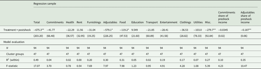
Notes: In the above regression setup, there are two treatment groups, that is, treatment and control groups, and two periods that are separated by an income shock event, which happens at the start of the second year. The treatment group receives an income shock based on the after-tax income from the last 12 months. There are five subtreatment groups and each receives an income loss shock of 20 percent, 24 percent, 26 percent, 30 percent, or 32 percent. The five treatment groups are pooled together. We follow the definition of Chetty and Szeidl (Reference Chetty and Szeidl2007) for “commitments” and “adjustables” categories, and follow their Table 1 in identifying which expenses belong to each commitments and adjustables category. Expenses for health, rent, and furnishings belong to the commitments category, and the rest of the expenses belongs to the adjustables category. Since our definition of transportation includes gas and maintenance, and clothing includes personal care items, we assign these to the adjustables category. All regressions are fixed-effects (within) regressions with household-level fixed effects. Cluster–robust standard errors are in parentheses—clustered at the household level. Significance level: *p < 0.05, **p < 0.01, ***p < 0.001.
The above results are in conformity with the theoretical predictions of Chetty and Szeidl (Reference Chetty and Szeidl2007), that is, after a small income shock, households reduce the consumption expenses of adjustable goods. We find evidence in support of our first hypothesis (H1) for the following expenses: all adjustable goods (a reduction of ~$579), food (a reduction of ~$119), and miscellaneous (a reduction of ~$280). However, we do not find evidence in support of our first hypothesis (H1) for the following expenses: education, transportation, clothing, and utilities. Two key takeaways from the consumption analysis of farm households in our sample are as follows: (i) a small income shock results in a downward adjustment of total consumption expenses, with the adjustment primarily concentrated in the adjustables category and (ii) within the adjustables category, a reduction in consumption expenses emanates from food and miscellaneous subcategories. In the last two columns of Table 3, we also show the regression results for commitments' and adjustables' share of preshock income. Among treatment households, on average, adjustables' share of income reduces by a significant 18.7 percent, which is in sharp contrast to the insignificant reduction of commitments' share of income (3.45 percent).
Risk Behavior Before and After Income Shock
Our risk elicitation method before the income loss intervention is based on an 11-point Likert scale method of Dohmen et al. (Reference Dohmen, Falk, Huffman, Sunde, Schupp and Wagner2011), while the risk elicitation method after the intervention is based on the risky lottery choice method of Guiso, Sapienza, and Zingales (Reference Guiso, Sapienza and Zingales2018). The former and the latter risk elicitation methods provide measures of “relative risk aversion” and “absolute risk aversion,” respectively (Guiso, Sapienza, and Zingales Reference Guiso, Sapienza and Zingales2018).Footnote 10
Using an ordered logit specification for the relative risk aversion measure, we do not find any significant difference in risk-taking behavior between treatment and control producers (see Table 4). However, in an interval regression specification for the absolute risk-aversion measure, we find that, on average, the risk premium of treatment producers is about $2,307 higher than that of control producers after the income loss intervention. Since an increase in risk premium translates into an increase in absolute risk aversion, we find the evidence in support of our second hypothesis (H2). We also confirm that absolute risk aversion is decreasing in wealth (income) as argued by Arrow (Reference Arrow1971) and Pratt (Reference Pratt1964).
Table 4. Producers' Risk Aversion Before/After the Income Shock

Notes: As discussed in the text, the qualitative risk measure elicits producers' willingness to take risk in the financial domain, following the Dohmen et al. (Reference Dohmen, Falk, Huffman, Sunde, Schupp and Wagner2011) method. It is referred to as the measure of relative risk aversion in Guiso, Sapienza, and Zingales (Reference Guiso, Sapienza and Zingales2018), and we model it using an ordered logit specification. The quantitative risk measure elicits producers' certainty equivalent in the face of a risky lottery ($10,000 versus $0) with equal chances. The quantitative risk measure is referred to as the absolute risk aversion measure in Guiso, Sapienza, and Zingales (Reference Guiso, Sapienza and Zingales2018). We then calculate the risk premium of each producer, which is the expected value of the lottery less certainty equivalent amount ($5,000—CE). We use the interval regression method to model the risk premium of producers. The qualitative risk measure is presented at the beginning of the survey (before income shock), and the quantitative measure is presented toward the end of the survey, after the shock. We dropped four observations because of inconsistency in response to risk questions. Two producers selected five or less (i.e., risk-averse) on the Likert scale for the qualitative measure, but they are extremely risk lovers after the shock (having a risk premium of −4,000 or less). Two other producers started as high risk takers (choosing 9 and 10 on the Likert scale), which dropped by two points each when asked the same question after the shock; however, their choice of risk premium (−4,000 or less) shows no indication of drop in risk taking. Robust standard errors are in parentheses. Significance level: *p < 0.05, **p < 0.01, ***p < 0.001.
Discussion of Results
During the summer of 2019, when we started implementing the survey, the emotional state of Indiana farmers was mired with frustration due to the concurrent rainfalls, which postponed the growing season. The flooding in some Midwestern states like Nebraska cost many farm producers their year-long farm yields. Such erratic weather outcomes are to be expected due to climate change (IPCC 2018). In the agriculture sector, farm producers are the most vulnerable to the adverse effects of natural disasters. After a disaster's negative income shock, the impact on producers' household consumption and individual risk behavior cannot be discounted.
Due to a disaster's hypothetical income loss, the treatment producers in our study reduced their food and miscellaneous expenses by about $119 and $280, respectively. Each of these two downward adjustments is equal to ~21 percent of the expenses for the food and miscellaneous categories before the income loss, respectively. It is easy to adjust food and miscellaneous expenses during hard times, but they can have real consequences over producers' life. Meanwhile, a postdisaster increase in risk aversion can have implications for specialty producers' financial decisions. For instance, postdisaster farm investment can be critical for farm output and revenues, but an increase in producers' risk aversion would mean that they are not willing enough to take on farm investment.
In our study, we find that Indiana specialty producers have a moderate resiliency against natural disasters. When we compare the consumption and risk-taking findings in our study against the moderate resiliency of specialty producers in our study, it becomes clear that the producer households and their farm enterprises are vulnerable to natural disasters. On average, 42 percent of the total planted acres in our survey sample are insured, which is not quite high enough (appendix Table A4). We also learn that about 80 percent of producers' farms have been affected by extreme events at some point, but only 53 percent of producers engage in farm financial planning for worst times such as farm losses due to a natural disaster (appendix Table A4). Potential solutions for improving the resilience capacity of Indiana specialty producers could include (i) connecting producers with digital technologies to help them in predicting weather and climate risks and (ii) educating producers about farm risk management tools that could help them to proactively manage their farms.
Conclusion
Specialty crops play a vital role in the U.S. farm sector due to their contribution to farm income and U.S. households' nutrition. However, specialty crops' production involves more risk than commodity crops' production due to adverse weather shocks, specialty crops' low insurance coverage and low participation rates, labor shortages, and perishability of fresh produce. Also, it is mainly the small- and medium-sized producers who are easily exposed to the aforementioned risks and challenges. The objective of this study is twofold: first, to determine how specialty producers' household consumption responds to adverse income shock due to natural disasters, and second, to evaluate whether an income loss experience affects specialty producers' risk-taking behavior.
In this study, we focus on specialty producers in the Midwestern state of Indiana. We administered a split-sample survey in the second half of 2019, where we randomly assigned producers to treatments that vary the size of a hypothetical income shock due to natural disasters. We collected information on (i) producers' resiliency in the face of natural disasters, (ii) households' monthly consumption expenditures before and after an income loss of 20–32 percent due to natural disasters, and (iii) producers' risk preferences.
We find that farm households in our sample reduce their monthly expenses of food and miscellaneous categories by ~$119 and ~$280, respectively, after an income loss of 20–32 percent. We also find that our sample producers are less willing to take financial risks after an income loss experience, that is, they have decreasing absolute risk aversion. Finally, we find in our data that Indiana specialty producers have a moderate resilience capacity to withstand the adverse effects of natural disasters. Although specialty crops' production is risky and challenging, the good news is that specialty producers can become resilient and manage farm risk with sufficient knowledge and resources. We believe Indiana specialty producers would benefit from (i) farm financial planning for the worst times, (ii) immediate access to federal aid and commercial loans after natural disasters, (iii) high participation rate in federal crop insurance, (iv) investment in agriculture-related digital technologies, and (v) more research on vulnerability and adaptive capacity of specialty producers.
Supplementary material
The supplementary material for this article can be found at https://doi.org/10.1017/age.2021.2.
Data Availability Statement
Survey instruments are available through the supplementary materials section of the article.
Appendix
Table A1. Indiana Specialty Crop Producers’ Demographics
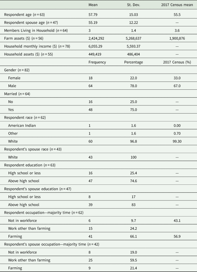
Table A2. Indiana Specialty Crop Producers Farm Operation Statistics

Table A3. Treatment/Control Balance—Household Income and Consumption Expenses Before the Income Shock
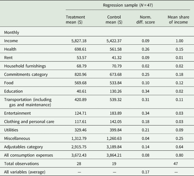
Table A4. Indiana Specialty Crop Producers' Resiliency Against Natural Disasters


 Open access