


Introduction
Evidence of racial disparities in policing is an urgent and highly relevant policy question in empirical research. A growing number of studies have focused on this critical topic (Baumgartner, Epp, and Shoub Reference Baumgartner, Epp and Shoub2018; Christiani et al. Reference Christiani, Shoub, Baumgartner, Epp and Roach2021; Eckhouse Reference Eckhouse2017; Edwards, Lee, and Esposito Reference Edwards, Lee and Esposito2019; Epp and Erhardt Reference Epp and Erhardt2020; Shoub et al. Reference Shoub, Epp, Baumgartner, Christiani and Roach2020). However, studies of racial disparities are fraught with methodological challenges (Goel, Rao, and Shroff Reference Goel, Rao and Shroff2016; Ridgeway Reference Ridgeway2006; Ridgeway and MacDonald Reference Ridgeway and MacDonald2009). Recent work by Knox, Lowe, and Mummolo (Reference Knox, Lowe and Mummolo2020, hereafter KLM) provides important new results on the difficulties of learning about racial disparities in policing from administrative data. One key point made by KLM is that such investigations have an intrinsic selection bias because administrative records only contain those encounters in which civilians are detained. If there is racial discrimination in police detainment in the first place, any naive analysis using the administrative data may then suffer from potentially severe selection bias.
Here, we present a research note on this important topic with two purposes. First, KLM focused on several local causal estimands that are being used in the empirical studies. We demonstrate that these local estimands—even when identified with observational data—cannot be used to make inferences about more global effects like the average treatment effect. Second, we introduce a global causal risk ratio estimand that is straightforward to interpret and requires fewer assumptions to identify than either the local effects considered by KLM or global risk differences. Although it still depends on some quantities that need to be estimated from external data, we demonstrate how we can use Bayes’ formula to avoid the hard problem of estimating the probability of detainment in police–civilian encounters. We conclude this research note with a reanalysis of the New York City Police Department (NYPD) Stop-and-Frisk dataset and some further discussion. Our empirical results show that a naive analysis of police administrative datasets that ignores the selection bias can severely underestimate the risk of police force for minorities. We present results that suggest a naive approach may understate the effect of civilian race on risk of police violence by a factor of 10 or more.
Review
We begin with a brief review of the key quantities in KLM. Following their work, the unit of analysis is an encounter between civilians and police, where an encounter is defined as all events in which the police sight a civilian, including those in which a civilian is allowed to pass undisturbed. There are n encounters indexed by I = 1,…,n. We denote the outcome with Yi , where Yi = 1 indicates the use of force by the police in encounter i. Next, Di is a binary variable where Di = 1 records the race of the civilian as a minority. While the race of the civilian is not manipulable, we adopt the approach in KLM where the counterfactual is the replacement of the civilian in an encounter with a separate, comparable civilian engaged in comparable behavior, but differing on race (Knox, Lowe, and Mummolo Reference Knox, Lowe and Mummolo2020, 621). We use Mi to indicate a police detainment or stop of a civilian. Critically, Mi = 1 for the subset of encounters that resulted in a stop by the police and are present in the administrative data. Finally, Xi represents a collection of covariates that describe aspects of the stops in the data. These could include measures for time of day, location, age, sex, and civilian behavior at the time when first encountered by police. Unless stated otherwise, conditioning on X is implicit.
For formal causal inference, we introduce the potential outcomes for Mi and Yi. We have the potential mediator Mi (d), which represents whether encounter i would have resulted in a stop if civilian race is d. Next, Yi (d,m) is the potential outcome for the use of force if race is d and the mediating variable is set to m; similarly, Yi (d) is the potential outcome if race is d. Throughout this note we make the stable unit treatment assumption (SUTVA), so Mi (Di ) = Mi and Yi (Di ,Mi ) = Yi (Di ) = Yi. This assumption means that the observed mediator (detainment) and outcome (use of force) are consistent with their corresponding counterfactual values. Hereafter, we assume the variables Di ,Mi , and Yi and the potential outcomes of Mi and Yi are drawn independently from the same unknown distribution. To simplify the exposition, we will drop the i subscript.
KLM studied the following “naive” treatment effect estimand:
 $$ \Delta =\unicode{x1D53C}\left[Y|D=1,M=1\right]-\unicode{x1D53C}\left[Y|D=0,M=1\right], $$
where
 $ \unicode{x1D53C} $
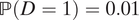
denotes expectation over a random police–civilian encounter. Intuitively, ∆ compares the average rates of force between different racial groups who are detained by police. KLM showed that, if there is racial discrimination in detainment and an unmeasured confounder between detainment and use of force (see Figure 1), the naive treatment effect ∆ can be quite misleading when used to represent the causal effect of race on police violence.
$ \unicode{x1D53C} $
denotes expectation over a random police–civilian encounter. Intuitively, ∆ compares the average rates of force between different racial groups who are detained by police. KLM showed that, if there is racial discrimination in detainment and an unmeasured confounder between detainment and use of force (see Figure 1), the naive treatment effect ∆ can be quite misleading when used to represent the causal effect of race on police violence.
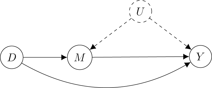
Figure 1. KLM’s Directed Acyclic Graph (DAG) Model for Racial Discrimination in Policing with an Unmeasured Mediator-Outcome Confounder U
Note:The treatment D is race of the civilian. The mediator M is an indicator for police detainment and the outcome Y is an indicator for police use of force. Administrative records only contain observations with M = 1.
The key issue is that the structure of the data implies all estimates are conditional on M—a posttreatment variable, which often leads to biased estimators of the causal effect (Rosenbaum Reference Rosenbaum1984). Bias of this type occurs in many applied problems in social science (Elwert and Winship Reference Elwert and Winship2014; Montgomery, Nyhan, and Torres Reference Montgomery, Nyhan and Torres2018) and medicine (Paternoster, Tilling, and Davey Smith Reference Paternoster, Tilling and Smith2017).
Using the principal stratification framework of Frangakis and Rubin (Reference Frangakis and Rubin2002), KLM showed that it is still possible to either identify or partially identify certain forms of average treatment effects using a set of tailored causal assumptions. These assumptions include mandatory reporting, mediator monotonicity, and treatment ignorability. Specifically, KLM derived nonparametric bounds for the average treatment effect of race on use of force among those who are detained by the police:
 $$ {\mathrm{ATE}}_{M=1}=\unicode{x1D53C}\left[Y(1)-Y(0)|M=1\right]. $$
They also derived a point identification formula for the average treatment effect among those who are minorities and detained by the police:
 $$ {\mathrm{ATT}}_{M=1}=\unicode{x1D53C}\left[Y(1)-Y(0)|D=1,M=1\right]. $$
Notice that their results rely on an external estimate of the proportion of racially motivated detainments among all reported minority detainments—that is,
 $ \mathrm{\mathbb{P}}\left(M(0)=0|D=1,M=1\right) $
. See KLM (631) for a discussion on estimating this quantity. Moreover, KLM also derived an identification formula for the average treatment effect
$ \mathrm{\mathbb{P}}\left(M(0)=0|D=1,M=1\right) $
. See KLM (631) for a discussion on estimating this quantity. Moreover, KLM also derived an identification formula for the average treatment effect
 $ \mathrm{ATE}=\unicode{x1D53C}\left[Y(1)-Y(0)\right] $
given external estimates of the rate of detainments
$ \mathrm{ATE}=\unicode{x1D53C}\left[Y(1)-Y(0)\right] $
given external estimates of the rate of detainments
 $ \mathrm{\mathbb{P}}\left(M=1|D=d\right) $
by race d = 0,1.
$ \mathrm{\mathbb{P}}\left(M=1|D=d\right) $
by race d = 0,1.
The identification results in KLM depend crucially on the following assumption:
Assumption 1 (Mandatory reporting). (i) Y(0,0) = Y(1,0) = 0 and (ii) the administrative data contains all detainments/stops of civilians by the police.
The first part of this assumption assumes that there will be no police violence if the civilian is not stopped in the first place. The second part assumes we observe a sample from the conditional distribution of the variables given M = 1, which is essential for statistical inference. We will make Assumption 1 throughout this note and further discuss its practical implications before the real data analysis.
Average Treatment Effects Conditional on the Mediator
In many causal analyses, investigators are focused on the sample average treatment effect (ATE), which is the average difference in potential outcomes averaged over the study population. At times, researchers define the ATE over specific subpopulations, which makes the ATE more local; for example, the average treatment effect might be defined for the subpopulation exposed to the treatment or the average treatment effect on the treated (ATT). Often the “global” ATE is the goal in many studies and is preferred over more local effects (Gerber and Green Reference Gerber and Green2012, chap. 2). For example, IV studies have been strongly critiqued for identifying a local average treatment effect (LATE) instead of the global ATE (Deaton Reference Deaton2010; Swanson and Hernán Reference Swanson and Hernán2014). Moreover, even some defenders of IV studies view the LATE as a “second choice” estimand compared with the global ATE (Imbens Reference Imbens2014).
As KLM outlined, the global ATE has not generally been the target causal estimand in this literature. Instead, researchers have focused on ATE
M=1 and ATT
M=1 which are both conditional on the mediator M. Notice that these estimands not only are more local than the global ATE but also condition on a posttreatment quantity. Nonetheless, they are not the first estimands in causal inference that condition on posttreatment quantities. Other examples of estimands that condition on posttreatment quantities include the survivor average treatment effect in Frangakis and Rubin (Reference Frangakis and Rubin2002) (though conceptually the always survivor principal stratum can be thought as a pretreatment variable), effect modification by a posttreatment quantity (Ertefaie et al. Reference Ertefaie, Hsu, Page and Small2018; Stephens, Keele, and Joffe Reference Stephens, Keele and Joffe2016), and the probability of causation
 $ \mathrm{\mathbb{P}}\left[Y(0)=0|D=1,Y=1\right] $
(Dawid, Musio, and Murtas Reference Dawid, Musio and Murtas2017; Pearl Reference Pearl1999; Robins and Greenland Reference Robins and Greenland1989).
$ \mathrm{\mathbb{P}}\left[Y(0)=0|D=1,Y=1\right] $
(Dawid, Musio, and Murtas Reference Dawid, Musio and Murtas2017; Pearl Reference Pearl1999; Robins and Greenland Reference Robins and Greenland1989).
The local effects in this context may have important policy relevance. As such, the preference for a global ATE may not always be warranted in this domain. However, an inexperienced researcher might think these local estimands are informative about the global ATE or even an estimand such as the controlled direct effect:
 $ \unicode{x1D53C}\left[Y\left(1,1\right)-Y\left(0,1\right)\right] $
. Next, we build upon the population stratification framework in KLM and clarify the difference between the conditional estimands in KLM and estimands like the global ATE.
$ \unicode{x1D53C}\left[Y\left(1,1\right)-Y\left(0,1\right)\right] $
. Next, we build upon the population stratification framework in KLM and clarify the difference between the conditional estimands in KLM and estimands like the global ATE.
To simplify the illustration, we will consider the case where there is no mediator-outcome confounder (i.e., no variable U in the diagram in Figure 1). The issues we describe below will still occur if there is mediator-outcome confounding. In mediation analysis, a standard way to decompose the average treatment effect is
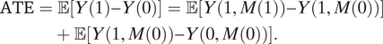 $$\begin{align}\mathrm{ATE}& =\unicode{x1D53C}\left[Y(1)-Y(0)\right]=\unicode{x1D53C}\left[Y\left(1,M(1)\right)-Y\left(1,M(0)\right)\right]\\&\quad+\unicode{x1D53C}\left[Y\left(1,M(0)\right)-Y\left(0,M(0)\right)\right].\end{align}$$
The two terms on the right-hand side are called the pure indirect effect (PIE) and pure direct effect (PDE; Robins and Greenland Reference Robins and Greenland1992). Under the nonparametric structural equation model with indeendent errors model (Pearl Reference Pearl2009; Richardson and Robins Reference Richardson and Robins2013) and Assumption 1, they can be expressed as (See the Appendix section A)
 $$ \mathrm{PIE}={\beta}_M\cdot \unicode{x1D53C}\left[Y\left(1,1\right)\right],\mathrm{PDE}={\beta}_Y\cdot \unicode{x1D53C}\left[M(0)\right], $$
where
 $ {\beta}_M=\unicode{x1D53C}\left[M(1)-M(0)\right] $
is the average effect of race on detainment and
$ {\beta}_M=\unicode{x1D53C}\left[M(1)-M(0)\right] $
is the average effect of race on detainment and
 $ {\beta}_Y=\unicode{x1D53C}\left[Y\left(1,1\right)-Y\left(0,1\right)\right] $
is the controlled direct effect of race on police violence. An immediate consequence of the above expressions is that
$ {\beta}_Y=\unicode{x1D53C}\left[Y\left(1,1\right)-Y\left(0,1\right)\right] $
is the controlled direct effect of race on police violence. An immediate consequence of the above expressions is that
 $$ \mathrm{ATE}\hskip2pt \ge \hskip2pt 0\hskip2pt \mathrm{if}\hskip2pt {\beta}_M,{\beta}_Y\hskip2pt \ge \hskip2pt 0\hskip0.5em \mathrm{and}\hskip0.5em \mathrm{ATE}\hskip2pt \le \hskip2pt 0\hskip2pt \mathrm{if}\hskip2pt {\beta}_M,{\beta}_Y\hskip2pt \le \hskip2pt 0. $$
In words, the global ATE is nonnegative whenever both the direct and indirect effects are nonnegative, and vice versa. This property also holds for the ATT because in the simple setting here the treatment D is completely randomized.
In the Appendix, we use principal stratification to show that neither ATE M=1 or ATT M=1 is guaranteed to inherit the sign of βM and βY and satisfy the property in Equation 2. Specifically, we outline concrete examples in which
-
(i) The pure direct and indirect effects are both positive, but ATE M=1 < 0;
-
(ii) The pure direct and indirect effects are both negative, but ATE M=1 > 0 and ATT M=1 > 0.
That is, when there is racial discrimination of the same direction in both police detainment and the use of force, it is still possible for ATE M=1 and ATT M=1 to have the opposite sign. We refer the reader to the Appendix for some concrete counterexamples and further comments on this phenomenon.
In sum, the local estimands ATE M=1 and ATT M=1 are generally different from the global estimands that are routinely the target in causal analyses. As such, we urge applied researchers to use caution when using these local estimands to infer anything about the global estimands.
A New Estimator for the Causal rRisk Ratio
KLM also derived an identification formula for ATE
M=1 using external estimates of the rate of detainment
 $ \mathrm{\mathbb{P}}\left(M=1|D=d\right) $
for race d = 0,1. Unfortunately, it is often difficult to quantify the frequency of stops among all police–civilian encounters, as noted in their paper. In particular, it can be difficult to determine the magnitude of
$ \mathrm{\mathbb{P}}\left(M=1|D=d\right) $
for race d = 0,1. Unfortunately, it is often difficult to quantify the frequency of stops among all police–civilian encounters, as noted in their paper. In particular, it can be difficult to determine the magnitude of
 $ \mathrm{\mathbb{P}}\left(M=1|D=d\right) $
. Here, we show that by formulating the estimand on a relative scale, we can avoid this difficulty and obtain point identification.
$ \mathrm{\mathbb{P}}\left(M=1|D=d\right) $
. Here, we show that by formulating the estimand on a relative scale, we can avoid this difficulty and obtain point identification.
More specifically, we consider the following causal risk ratio (CRR) for covariate level x:
 $$ \mathrm{CRR}(x)=\frac{\unicode{x1D53C}\left[Y(1)|X=x\right]}{\unicode{x1D53C}\left[Y(0)|X=x\right]}. $$
When this term is equal to one, the risk of police violence does not vary with the race of the civilian. When this term is greater than one, the risk of violence is higher for minorities. Risk ratios, while not commonly used in political science, have been used in the literature on policing (Christiani et al. Reference Christiani, Shoub, Baumgartner, Epp and Roach2021; Eckhouse Reference Eckhouse2017; Edwards, Lee, and Esposito Reference Edwards, Lee and Esposito2019). However, previous researchers that use risk ratios have tended to present them as descriptive values rather than as causal quantities. Moreover, risk ratios can be a powerful rhetorical tool for understanding discussions of racial disparities. In the context of police violence, it may be tempting to use the following ratio to measure racial disparities:
 $$ \mathrm{Naive}\hskip0.5em \mathrm{risk}\hskip0.5em \mathrm{ratio}=\frac{\unicode{x1D53C}\left[Y|D=1,M=1,X=x\right]}{\unicode{x1D53C}\left[Y|D=0,M=1,X=x\right]}. $$
This quantity divides the rates of police violence experienced by minorities and nonminorities, given that they have the same covariate x and are detained by the police. We will see below that the naive risk ratio is generally not the same as the causal risk ratio due to conditioning on the colliding variable M (detainment); in fact, these two quantities can be drastically different.
Expressing results in a relative fashion can be an effective way of communication, especially when the risk of police violence is fairly low among a specific population. For example, let’s say in one specific locale, the risk of police violence for Black residents is 0.01% and is 0.001% for white residents. The difference in these risks is obviously very small. However, in relative terms, the risk of police violence for Black residents is 10 times that for white residents. As such, even if the absolute risk is low, a large increase in relative risk is likely to be of significant interest.
Using treatment ignorability (i.e., the DAG model in Figure 1 conditional on X) and Assumption 1, the causal effect of race can be identified based on the decomposition
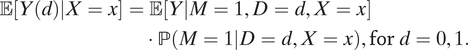 $$ \begin{align}\unicode{x1D53C}\left[Y(d)|X=x\right] &= \unicode{x1D53C}\left[Y|M=1,D=d,X=x\right]\\ &\cdot \mathrm{\mathbb{P}}\left(M=1|D=d,X=x\right),\mathrm{for}\hskip2.5pt d=0,1.\end{align} $$
The same result is derived in KLM and forms the basis of their identification of the ATE. We simplify their proof in the Appendix and show that some of KLM’s identification assumptions can be relaxed. Specifically, we can arrive at the same result without invoking mediator monotonicity and relative nonseverity of racial stops (Assumptions 2 and 3 in KLM).
By using Bayes formula for the last term on the right hand side (see the Appendix), we obtain the following identification result:
 $$ \begin{align}\mathrm{CRR}(x)&=\underset{\mathrm{naive}\hskip0.5em \mathrm{risk}\hskip0.5em \mathrm{ratio}}{\underbrace{\frac{\unicode{x1D53C}\left[Y|D=1,M=1,X=x\right]}{\unicode{x1D53C}\left[Y|D=0,M=1,X=x\right]}}}\\ &\underset{\mathrm{bias}\hskip0.5em \mathrm{factor}}{\underbrace{\cdot\left\{\frac{\mathrm{\mathbb{P}}\left(D=1|M=1,X=x\right)}{\mathrm{\mathbb{P}}\left(D=0|M=1,X=x\right)}\right\}/\left\{\frac{\mathrm{\mathbb{P}}\left(D=1|X=x\right)}{\mathrm{\mathbb{P}}\left(D=0|X=x\right)}\right\}}}.\end{align} $$
Therefore, by targeting the causal risk ratio, we are able to avoid the difficulties associated with estimating the absolute rate of detainment
 $ \mathrm{\mathbb{P}}\left(M=1\right) $
through cancellation.
$ \mathrm{\mathbb{P}}\left(M=1\right) $
through cancellation.
The first term on the right-hand side of Equation 3 is the naive risk ratio estimand conditional on baseline covariates. It is the risk ratio counterpart to the naive risk difference in Equation 1, and both of them ignore the possible bias from the selection process into the administrative data. The second term inside the curly brackets is a ratio of probability ratios. The first ratio of probabilities measures the relative probability of a detainment being with a minority conditional on covariate X = x, which can be estimated from the administrative data. The second ratio measures the relative probability (odds) of an encounter being with a minority conditional on covariate X = x, but these probabilities need to be approximated or bounded with a second data source. This ratio between the last two terms is thus an odds ratio that characterizes the bias of the naive estimator; for this reason, we call it the “bias factor.” That is, if minorities are overrepresented in the administrative data, the bias factor corrects that overrepresentation and so increases the magnitude of the risk ratio. For example, if the probability of a detainment being with a minority is 0.8 in the administrative data and 0.25 in a random police–civilian encounter, the bias factor would be (0.8/0.2) / (0.25/0.75) = 12, which would increase the magnitude of the naive risk ratio when it is larger than 1. All the terms in Equation 3 can be estimated using generalized linear models (such as logistic regression) or more flexible models. Confidence intervals can be estimated using the bootstrap or the delta method.
Note that if we are willing to assume stochastic mediator monotonicity:
 $ \unicode{x1D53C}\left[M(1)|X=x\right]\hskip2pt \ge \hskip2pt \unicode{x1D53C}\left[M(0)|X=x\right] $
(i.e., there is racial bias against the minority in detainment), the bias factor can indeed be lower bounded by 1. In this case, the naive risk ratio (first term on the right hand side of Equation 3) provides a lower bound for the causal risk ratio CRR(x).
$ \unicode{x1D53C}\left[M(1)|X=x\right]\hskip2pt \ge \hskip2pt \unicode{x1D53C}\left[M(0)|X=x\right] $
(i.e., there is racial bias against the minority in detainment), the bias factor can indeed be lower bounded by 1. In this case, the naive risk ratio (first term on the right hand side of Equation 3) provides a lower bound for the causal risk ratio CRR(x).
While the risk ratio estimand does avoid Assumptions 2 and 3 in KLM critical complications are still present. That is, the constraints that tend to arise from the use of two data sources remain a significant source of complexity. In particular, the administrative dataset can only be used to estimate the first two terms on the right hand side of Equation 3. We must find an additional data source that allows us to estimate the racial distribution conditional on the covariates—
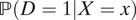 $ \mathrm{\mathbb{P}}\left(D=1|X=x\right) $
and
$ \mathrm{\mathbb{P}}\left(D=1|X=x\right) $
and
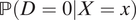 $ \mathrm{\mathbb{P}}\left(D=0|X=x\right) $
—since the administrative data only contain those encounters where M = 1. However, secondary data sources tend to also contain data on stops rather than encounters (sightings of civilians by the police). As such, typically, we use population level data on police stops to approximate encounter rates by racial group. To the extent that these quantities are proportional, the method will be accurate. However, to the extent that these quantities differ, the measure will be biased. Moreover, there may be measurement inconsistencies between the secondary data and the administrative data. This can be partly addressed by a sensitivity analysis; see the next section for an example. See also Knox and Mummolo (Reference Knox and Mummolo2020) for further discussion on the usage of external datasets in this context.
$ \mathrm{\mathbb{P}}\left(D=0|X=x\right) $
—since the administrative data only contain those encounters where M = 1. However, secondary data sources tend to also contain data on stops rather than encounters (sightings of civilians by the police). As such, typically, we use population level data on police stops to approximate encounter rates by racial group. To the extent that these quantities are proportional, the method will be accurate. However, to the extent that these quantities differ, the measure will be biased. Moreover, there may be measurement inconsistencies between the secondary data and the administrative data. This can be partly addressed by a sensitivity analysis; see the next section for an example. See also Knox and Mummolo (Reference Knox and Mummolo2020) for further discussion on the usage of external datasets in this context.
Take the NYPD database of police stops as an example. This data source was used in KLM and will be reanalyzed in the next section. For a second data source, we will use the Current Population Survey (CPS), which contains measures for race and also has geographic information that allows us to restrict the data to the metro area in the state of New York (which is larger than the five boroughs of New York City). However, The CPS does not contain any more fine-grained geographic identifiers or any measures of police encounters or stops. Another data source we will use is the Police-Public Contact Survey (PPCS) collected by the U.S. Department of Justice. However, PPCS is a national survey and geographic identifiers are not available to researchers. As such, if we use the PPCS, we can do little to measure the prevalence of police–minority interactions in New York City. Additionally, the PPCS collects data on police stops and not encounters. As such, we cannot measure rates of encounters with either data source.
In other settings such as traffic stops, one may use the “veil of darkness” test (Grogger and Ridgeway Reference Grogger and Ridgeway2006) and use nighttime police stops in the same dataset to estimate the bias factor, as police are less likely to know the race of a motorist. However, this still requires the assumption that the racial distribution of motorists is the same during the day and at night. Moreover, data sources on encounters are exceedingly rare, and despite the limitations, as we show next, the results using the risk ratio with different data sources can still be useful and illuminate the probable bias in the naive estimator. They can also serve as the baseline of a sensitivity analysis.
We conclude this section, with a final comment on data constraints. Identification of the risk ratio estimand as well as those derived in KLM depend on mandatory reporting (Assumption 1). It is important to note that this assumption is both a restriction on potential outcomes and a feature of the data collection. The first part of the assumption says that the potential outcome Y(d,m) is equal to 0 whenever m = 0. This assumption is reasonable because, besides inadvertent collateral damage, there should be virtually no police violence if the civilian is not stopped by the police in the first place. The second part of the assumption is needed so that we can use the administrative dataset to get the conditional distribution of (D,Y,X) given M = 1. For a given administrative data source, it is possible that some police stops are unrecorded. If that is the case, any analysis relying on Assumption 1 needs to be interpreted with care. This is not a major concern in the NYPD dataset reanalyzed below, as all NYPD police officers are required to report all the stops.
A Reanalysis of the NYPD Stop-and-Frisk Dataset
We used the identification formula in Equation 3 to estimate the causal risk ratio using the NYPD “Stop-and-Frisk” dataset analyzed in Fryer (Reference Fryer2019) and KLM. Specifically, we use the replication data from KLM. As such, we followed KLM’s preprocessing of the dataset, with the one exception that we removed all races other than Black and white. We also focused on all forms of force rather than estimate the effects for different types of force. We used CPS 2013 and PPCS 2011 data to estimate the third term in Equation 3. See the end of this section for a sensitivity analysis where we perturb the estimates from census data. Because PPCS does not contain a geographic identifier, we also used the racial distributions for different subsets of the PPCS data. Specifically, we used subgroups for those in the survey that experienced a motor vehicle stop, any other kind of police stop, and those in a large metro area. We further explored weighting the PPCS respondents by their reported number of face-to-face contacts with the police. Respondents with more than 30 reported contacts with the police were excluded in that analysis. See the Appendix section C for details on the exact survey items we used in this analysis. As we noted above, neither CPS or PPCSD records police–civilian encounters per our definition (sighting of civilians), so they can only be regarded as approximations of the actual racial distribution in encounters.
Table 1 reports the estimated risk ratios using different estimators and external datasets. Using the naive estimator—the first term in Equation 3, we find a modest causal effect: Black people have 29% higher risk of the police using force than white people. Recall that we can view this as lower bound on the true causal risk ratio if we are willing to assume stochastic mediator monotonicity (i.e., there is discrimination against Black civilians in police detainments on average). The estimator from Equation 3 that adjusts for the selection bias shows a very different picture. No matter which external dataset we used, the estimated risk ratio for Black versus white is always greater than 10.
Table 1. Estimates of the Causal Effect of Minority Race (Black) on Police Violence
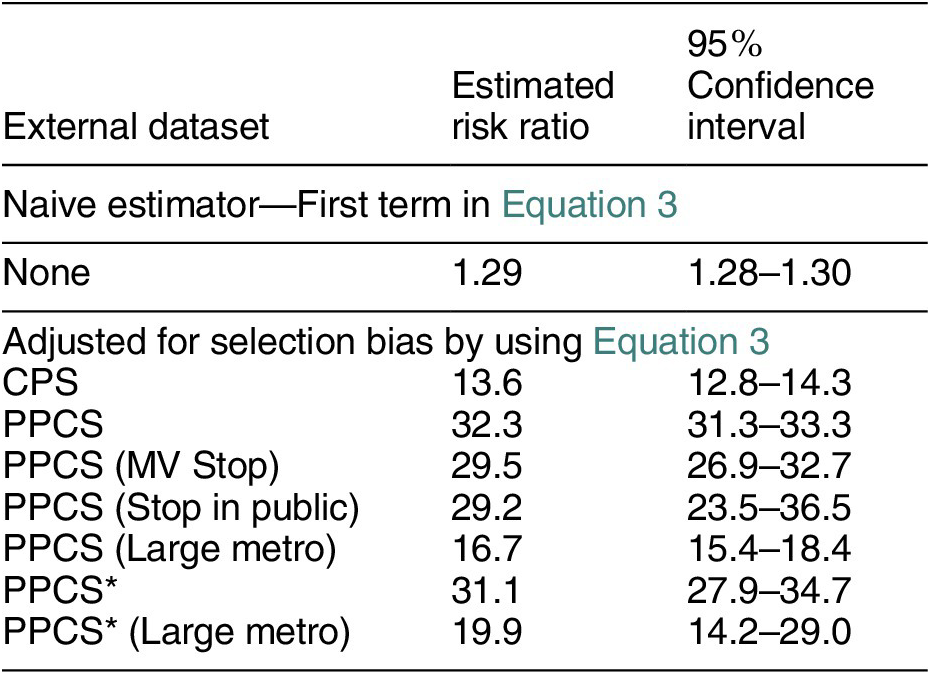
Note: CPS is the Current Population Survey. PPCS is Police-Public Contact Survey. PPCS* is PPCS, with the respondents weighted by their reported number of face-to-face contacts with the police. MV Stop is the subset of survey respondents that has been the passenger in a motor vehicle that was stopped by the police. Large Metro is the subset that lives in a region with more than 1 million population. Confidence intervals were computed using the nonparametric bootstrap.
The estimates in Table 1 did not condition on any covariate that confounds the effect of race on police use of force. In the Appendix section D, we report the results of a stratified analysis by age and gender of the civilian. The estimates are broadly consistent with those reported in Table 1, but it appears that female minorities have a much smaller risk ratio (less discriminated against) than male minorities. Age does not appear to be an important effect modifier.
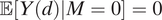
Another potentially important confounder is the location of the police–civilian encounter. However, detailed geographic information is not available in CPS or PPCS. The NYPD currently has 77 precincts that are responsible for the law enforcement within a designated geographic area. Using census blocks and the 2010 census data, Keefe (Reference Keefe2020) constructed a population breakdown for each NYPD precinct. This allows us to compare the proportion of Black residents (among Black and white residents) with the proportion of detainments of Black civilians in each precinct (Figure 2). It is evident from this figure that in most of the precincts, Black civilians make up less than half of the population but more than half of the detainment records. This shows that the bias factor in Equation 3 can be quite large in this problem.
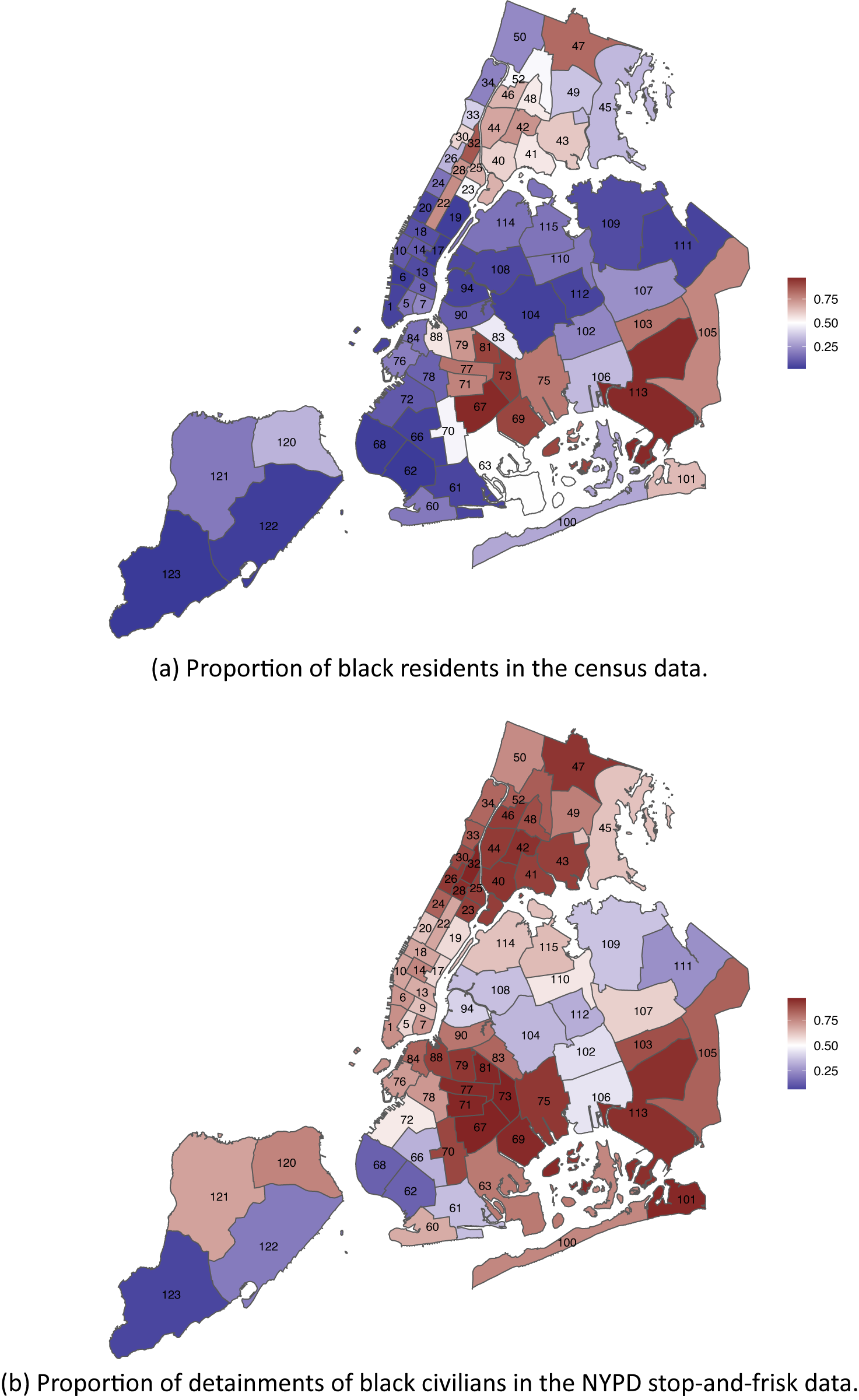
Figure 2. Racial Distributions (Indicated by the Filled Color) in Each NYPD Precinct
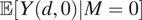
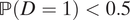
By using the census data to estimate the last term in Equation 3, Figure 3 compares the naive risk ratio estimator and selection-adjusted risk ratio estimator for each precinct. The selection-adjusted estimates are almost always much larger except for three outliers—precincts 67 and 113, where Blacks account for more than 90% of the population, and precinct 22 (Central Park), where only 25 residents were recorded and the majority of police–civilian encounters were likely with nonresidents. It is likely that in these precincts, the residential distribution in the census data poorly approximate the racial distribution in police–civilian encounters because the civilians could be visitors from other precincts or anywhere else in the world. Most of the precincts with the highest estimated risk ratios are wealthy neighborhoods in Manhattan and Brooklyn. In several precincts, our method estimated that the risk of police use of force for Blacks is more than 30 times higher than the risk for whites. This may be due in part to increased suspicion of minorities in areas where there presence is not common. Finally, Figure 4a shows a strong negative correlation between the estimated risk ratios and the percentage of Black residents in the precinct. This indicates that the racial discrimination in police use of force may be strongly moderated by characteristics of the geographic location such as the racial composition, affluence, and average crime rate of the neighborhood.
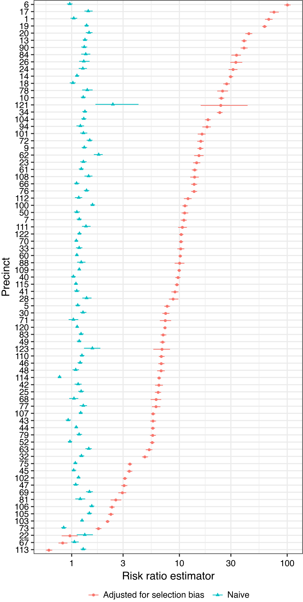
Figure 3. Risk Ratio Estimates for Every NYPD Precinct
Note: The error bars correspond to 95% confidence intervals computed by the bootstrap. We did not resample the census data because that is already the residential distribution (instead of a statistical estimate). The blue estimates are obtained by using the naive estimator, the first term in Equation 3; the red estimates further take into account the bias factor due to sample selection in Equation 3.
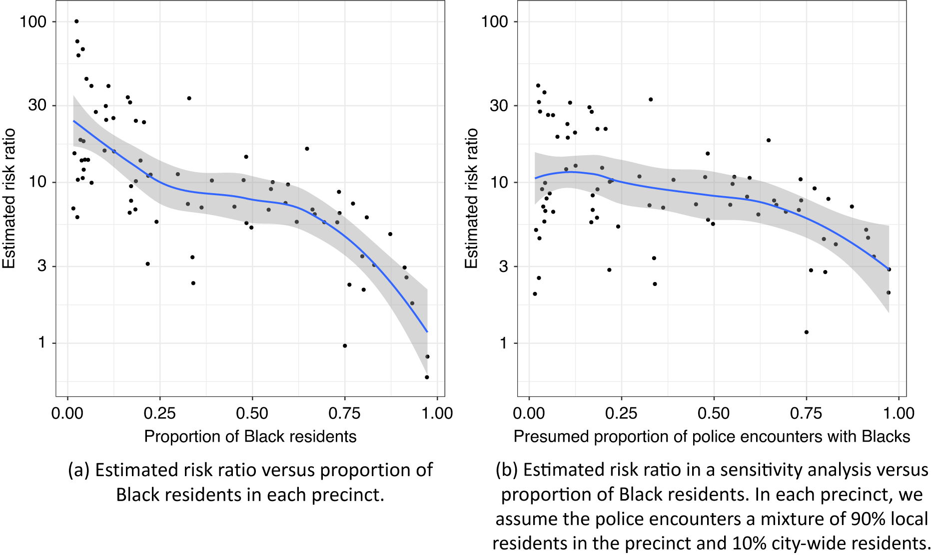
Figure 4. Estimated Risk Ratio versus Proportion of Black Residents in Each Precinct
The above analysis relies on the assumption that the racial distribution in police–civilian encounters can be well approximated by the racial distribution in census or survey datasets. A sensitivity analysis can be useful to gauge the potential bias due to poor approximations of the racial distribution in police–civilian encounters. Figure 4b presents such a sensitivity analysis, where the civilians who encountered the police are assumed to be a mixture of local and citywide residents. More precisely, this sensitivity analysis assumes that in each precinct, there is a 90% chance of the police encountering a local resident and a 10% chance of the police encountering a resident from another precinct. According to the census data, 36.7% of the population in New York City (excluding races other than Black and white) was Black in 2010. Thus, in this sensitivity analysis, the presumed proportion of encounters with Black civilians is higher than the proportion of Black residents in the precinct, if the proportion of Black residents is lower than 36.7%. This shrinks the estimated causal risk ratio towards a common value, especially for precincts that are predominantly white or predominantly Black, as shown in Figure 4b.
Conclusions
In this research note, we studied some causal estimands in the context of racial discrimination in policing. We found that the ATE that conditions on the mediator (police detainment) can differ in sign from the unconditional ATE and other routinely used causal estimands, so extra caution is needed when using these estimands and interpreting the results. We also proposed a new estimator for the causal risk ratio, which is straightforward to interpret and avoids the difficult task of discerning the percentage of stops in all police–civilian encounters. In a reanalysis of the NYPD Stop-and-Frisk dataset with causal risk ratio being the estimand, we found that for Blacks the risk of experiencing force is much higher than for whites.
When interpreting the results of our reanalysis, the reader should keep in mind its limitations. First, it is difficult to find a good external dataset to estimate the bias factor. The datasets we used should only be viewed as crude approximations to the racial distribution in police–civilian encounters in New York City. Second, our measure of the causal risk ratio is conditional on covariates X; identification requires treatment ignorability conditional on confounders included in X. In principle, that would involve conditioning simultaneously on confounders like time, location, and other relevant characteristics of the police–civilian encounter. However, such covariates are not always available in external datasets and our analysis only conditions on NYPD precinct. Additionally, our method does not yet have a way to summarize over multiple covariate strata even if the conditional risk ratios are identified and estimated. Since we did not use visible features of the civilians that are associated with race and criminal activity (they are not available in the data), this may have led to overestimation of the effect of race on use of force. It is highly implausible that this bias could fully explain the large measures of association found here. Finally, since New York is a metropolitan in which people move around a great deal on a daily basis, the racial distribution of the residents in a precinct might poorly represent the racial distribution in police–civilian encounters, especially when the residential distribution is extreme, as demonstrated in our sensitivity analysis. In other words, Figure 4a may have exaggerated the effect modification by the racial distribution of the local residents. A further analysis on carefully selected precincts (e.g., residential areas with different racial compositions) is needed to better quantify the effect modification.
Nevertheless, our empirical results show that a naive analysis of police administrative datasets that ignores the selection bias can severely underestimate the risk of police force for minorities. This also highlights the importance of defining the causal estimand clearly in observational studies. Further careful analyses are needed to better quantify the racial discrimination in policing and understand the socioeconomic factors that moderate racial discrimination.
Finally, we offer a concrete suggestion for applied analysts based on our results. KLM conclude by outlining a feasible research design for policing studies. Our risk-ratio-based analysis and the associated sensitivity analysis are useful additions to their suggested research plan. Our methods provide useful complements to the analyses outlined by KLM. Any policing study will depend on strong assumptions and a broad set of results that agree will provide higher quality evidence.
Supplementary Materials
To view supplementary material for this article, please visit http://doi.org/10.1017/S0003055421000654.
Data Availability Statement
Research data that support the findings of this study are openly available at the American Political Science Review Dataverse: https://doi.org/10.7910/DVN/ZQMYII.
Acknowledgments
The authors thank Dean Knox, Joshua Loftus, Jonathan Mummolo, and four anonymous reviewers for their helpful suggestions.
Conflict of Interest
The authors declare no ethical issues or conflicts of interest in this research.
Ethical Standards
The authors affirm this research did not involve human participants.
Appendix
A Note on Posttreatment Selection in Studying Racial Discrimination in Policing
A Average Treatment Effects Conditional on the Mediator
We assume the variables (D,M,Y) are generated from a nonparametric structural equation model:
![]() , where
, where
![]() are mutually independent (Pearl Reference Pearl2009). Potential outcomes for M and Y can be defined by replacing random variables in the functions by fixed values; for example,
are mutually independent (Pearl Reference Pearl2009). Potential outcomes for M and Y can be defined by replacing random variables in the functions by fixed values; for example,
![]() . Because the errors are independent, D, {M(0), M(1)}, and {Y(0,0), Y(0,1), Y(1,0), Y(1,1)} are mutually independent (Richardson and Robins Reference Richardson and Robins2013). We also make the mandatory assumption (Assumption 1). The derivations below do not need mediator monotonicity (M(1) ≥ M(0)).
. Because the errors are independent, D, {M(0), M(1)}, and {Y(0,0), Y(0,1), Y(1,0), Y(1,1)} are mutually independent (Richardson and Robins Reference Richardson and Robins2013). We also make the mandatory assumption (Assumption 1). The derivations below do not need mediator monotonicity (M(1) ≥ M(0)).
We next derive expressions of ATE
M=1 and ATT
M=1 using two basic causal effects:
 $ {\beta}_M=\unicode{x1D53C}\left[M(1)-M(0)\right] $
, the racial bias in detainment, and
$ {\beta}_M=\unicode{x1D53C}\left[M(1)-M(0)\right] $
, the racial bias in detainment, and
 $ {\beta}_Y=\unicode{x1D53C}\left[Y\left(1,1\right)-Y\left(0,1\right)\right] $
, the controlled direct effect of race on police violence. To simplify the interpretation, we introduce a new variable to denote the the principal stratum (see Figure 2 in KLM):
$ {\beta}_Y=\unicode{x1D53C}\left[Y\left(1,1\right)-Y\left(0,1\right)\right] $
, the controlled direct effect of race on police violence. To simplify the interpretation, we introduce a new variable to denote the the principal stratum (see Figure 2 in KLM):
 $$ S=\left\{\begin{array}{ll}\mathrm{always}\ \mathrm{stop}\hskip2pt \left(\mathrm{al}\right),& \mathrm{if}\hskip2pt M(0)=M(1)=1,\\ {}\mathrm{minority}\ \mathrm{stop}\hskip2pt \left(\mathrm{mi}\right),& \mathrm{if}\hskip2pt M(0)=0,M(1)=1,\\ {}\mathrm{majority}\ \mathrm{stop}\hskip2pt \left(\mathrm{ma}\right),& \mathrm{if}\hskip2pt M(0)=1,M(1)=0,\\ {}\mathrm{never}\ \mathrm{stop}\hskip2pt \left(\mathrm{ne}\right),& \mathrm{if}\hskip2pt M(0)=M(1)=0,\end{array}\right. $$
Let S = {al, mi, ma, ne} be all possible values for S. Using this notation, we have
 $$ {\beta}_M=\sum \limits_{s\in \mathcal{S}}\unicode{x1D53C}\left[M(1)-M(0)|S=s\right]\mathrm{\mathbb{P}}\left(S=s\right)=\mathrm{\mathbb{P}}\left(S=\mathrm{mi}\right)-\mathrm{\mathbb{P}}\left(S=\mathrm{ma}\right). $$
By using the independence between M(d) and Y(d, m) and assump:m0y0, it is easy to show that
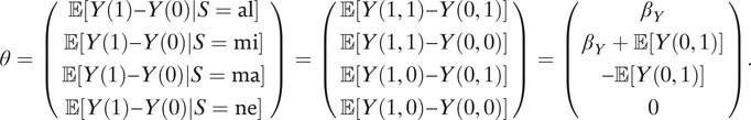 $$ \theta =\left(\begin{array}{c}\unicode{x1D53C}\left[Y(1)-Y(0)|S=\mathrm{al}\right]\\ {}\unicode{x1D53C}\left[Y(1)-Y(0)|S=\mathrm{mi}\right]\\ {}\unicode{x1D53C}\left[Y(1)-Y(0)|S=\mathrm{ma}\right]\\ {}\unicode{x1D53C}\left[Y(1)-Y(0)|S=\mathrm{ne}\right]\\ {}\end{array}\right)=\left(\begin{array}{c}\unicode{x1D53C}\left[Y\left(1,1\right)-Y\left(0,1\right)\right]\\ {}\unicode{x1D53C}\left[Y\left(1,1\right)-Y\left(0,0\right)\right]\\ {}\unicode{x1D53C}\left[Y\left(1,0\right)-Y\left(0,1\right)\right]\\ {}\unicode{x1D53C}\left[Y\left(1,0\right)-Y\left(0,0\right)\right]\\ {}\end{array}\right)=\left(\begin{array}{c}{\beta}_Y\\ {}{\beta}_Y+\unicode{x1D53C}\left[Y\left(0,1\right)\right]\\ {}-\unicode{x1D53C}\left[Y\left(0,1\right)\right]\\ {}0\\ {}\end{array}\right). $$
Average treatment effects, whether conditional on M or D or not, can be written as weighted averages of the entries of θ.
Proposition 1. Suppose there is no unmeasured mediator-outcome confounder (i.e., no U) in Figure 1. Under Assumption 1, the estimands ATE
M=1, ATT
M=1,
 $ \mathrm{ATE}=\unicode{x1D53C}\left[Y(1)-Y(0)\right] $
, and
$ \mathrm{ATE}=\unicode{x1D53C}\left[Y(1)-Y(0)\right] $
, and
 $ \mathrm{ATT}=\unicode{x1D53C}\left[Y(1)-Y(0)|D=1\right] $
can be written as weighted averages
$ \mathrm{ATT}=\unicode{x1D53C}\left[Y(1)-Y(0)|D=1\right] $
can be written as weighted averages
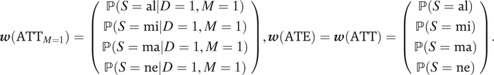
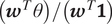 $ \left({\boldsymbol{w}}^T\theta \right)/\left({\boldsymbol{w}}^T\mathbf{1}\right) $
(1 is the all-ones vector) with weights given by, respectively,
$ \left({\boldsymbol{w}}^T\theta \right)/\left({\boldsymbol{w}}^T\mathbf{1}\right) $
(1 is the all-ones vector) with weights given by, respectively,
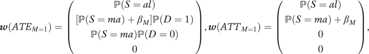 $$ \boldsymbol{w}\left({ATE}_{M=1}\right)=\left(\begin{array}{c}\mathrm{\mathbb{P}}\left(S= al\right)\\ {}\left[\mathrm{\mathbb{P}}\left(S= ma\right)+{\beta}_M\right]\mathrm{\mathbb{P}}\left(D=1\right)\\ {}\mathrm{\mathbb{P}}\left(S= ma\right)\mathrm{\mathbb{P}}\left(D=0\right)\\ {}0\\ {}\end{array}\right),\boldsymbol{w}\left({ATT}_{M=1}\right)=\left(\begin{array}{c}\mathrm{\mathbb{P}}\left(S= al\right)\\ {}\mathrm{\mathbb{P}}\left(S= ma\right)+{\beta}_M\\ {}0\\ {}0\\ {}\end{array}\right), $$
and
 $$ \boldsymbol{w}(ATE)=\boldsymbol{w}(ATT)=\left(\begin{array}{c}\mathrm{\mathbb{P}}\left(S= al\right)\\ {}\mathrm{\mathbb{P}}\left(S= mi\right)\\ {}\mathrm{\mathbb{P}}\left(S= ma\right)\\ {}\mathrm{\mathbb{P}}\left(S= ne\right)\\ {}\end{array}\right)=\left(\begin{array}{c}\mathrm{\mathbb{P}}\left(S= al\right)\\ {}\mathrm{\mathbb{P}}\left(S= ma\right)+{\beta}_M\\ {}\mathrm{\mathbb{P}}\left(S= ma\right)\\ {}\mathrm{\mathbb{P}}\left(S= ne\right)\\ {}\end{array}\right). $$
Proof. Let’s first consider ATE M=1. By using the law of total expectations, we can first decompose it into a weighted average of principal stratum effects:
 $$ {\mathrm{ATE}}_{M=1}=\unicode{x1D53C}\left[Y(1)-Y(0)|M=1\right]=\sum \limits_{s\in \mathcal{S}}\unicode{x1D53C}\left[Y(1)-Y(0)|M=1,S=s\right]\cdot \mathrm{\mathbb{P}}\left(S=s|M=1\right). $$
We can simplify the principal stratum effects using recursive substitution of the potential outcomes and the assumption that D, {M(0), M(1)}, and {Y(0,0), Y(0,1), Y(0,1), Y(1,1)} are mutually independent. For m 0, m 1 ϵ {0,1},
 $$ {\displaystyle \begin{array}{l}\unicode{x1D53C}\left[Y(1)-Y(0)|M=1,M(0)={m}_0,M(1)={m}_1\right]=\unicode{x1D53C}\left[Y\left(1,M(1)\right)-Y\left(0,M(0)\right)|M=1,M(0)={m}_0,M(1)={m}_1\right]\\ {}=\unicode{x1D53C}\left[Y\left(1,{m}_1\right)-Y\left(0,{m}_0\right)|M=1,M(0)={m}_0,M(1)={m}_1\right]\\ {}=\unicode{x1D53C}\left[Y\left(1,{m}_1\right)-Y\left(0,{m}_0\right)|M(0)={m}_0,M(1)={m}_1\right]\\ {}=\unicode{x1D53C}\left[Y\left(1,{m}_1\right)-Y\left(0,{m}_0\right)\right].\end{array}} $$
The third equality uses the fact that
 $ M\perp \left\{Y\left(1,{m}_1\right),Y\left(0,{m}_0\right)\right\}\mid \left\{M(0),M(1)\right\} $
because given {M (0), M (1)} the only random term in M = D M(1) + (1 − D) M(0) is D. Thus ATE
M=1 can be written as
$ M\perp \left\{Y\left(1,{m}_1\right),Y\left(0,{m}_0\right)\right\}\mid \left\{M(0),M(1)\right\} $
because given {M (0), M (1)} the only random term in M = D M(1) + (1 − D) M(0) is D. Thus ATE
M=1 can be written as
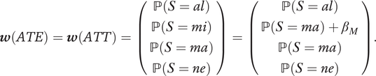
 $$ {\mathrm{ATE}}_{M=1}={\theta}^T\boldsymbol{w}\left({\mathrm{ATE}}_{M=1}\right),\mathrm{where}\hskip2pt \boldsymbol{w}\left({\mathrm{ATE}}_{M=1}\right)=\left(\begin{array}{c}\mathrm{\mathbb{P}}\left(S=\mathrm{al}|M=1\right)\\ {}\mathrm{\mathbb{P}}\left(S=\mathrm{mi}|M=1\right)\\ {}\mathrm{\mathbb{P}}\left(S=\mathrm{ma}|M=1\right)\\ {}\mathrm{\mathbb{P}}\left(S=\mathrm{ne}|M=1\right)\\ {}\end{array}\right). $$
Similarly, ATT M=1, ATE, and ATT can also be written as weighted averages of the entries of θ, where the weights are
 $$ \boldsymbol{w}\left({\mathrm{ATT}}_{M=1}\right)=\left(\begin{array}{c}\mathrm{\mathbb{P}}\left(S=\mathrm{al}|D=1,M=1\right)\\ {}\mathrm{\mathbb{P}}\left(S=\mathrm{mi}|D=1,M=1\right)\\ {}\mathrm{\mathbb{P}}\left(S=\mathrm{ma}|D=1,M=1\right)\\ {}\mathrm{\mathbb{P}}\left(S=\mathrm{ne}|D=1,M=1\right)\\ {}\end{array}\right),\boldsymbol{w}\left(\mathrm{ATE}\right)=\boldsymbol{w}\left(\mathrm{ATT}\right)=\left(\begin{array}{c}\mathrm{\mathbb{P}}\left(S=\mathrm{al}\right)\\ {}\mathrm{\mathbb{P}}\left(S=\mathrm{mi}\right)\\ {}\mathrm{\mathbb{P}}\left(S=\mathrm{ma}\right)\\ {}\mathrm{\mathbb{P}}\left(S=\mathrm{ne}\right)\\ {}\end{array}\right). $$
Next we compute the conditional probabilities for the principal strata in w(ATE M=1) and w(ATT M=1). By using Bayes’ formula, for any m 0, m 1ϵ{0,1},
 $$ {\displaystyle \begin{array}{l}\hskip.7em \mathrm{\mathbb{P}}\left(M(0)={m}_0,M(1)={m}_1|M=1\right)\\ {}\propto \hskip2pt \mathrm{\mathbb{P}}\left(M(0)={m}_0,M(1)={m}_1\right)\cdot \mathrm{\mathbb{P}}\left(M=1|M(0)={m}_0,M(1)={m}_1\right)\\ {}=\mathrm{\mathbb{P}}\left(M(0)={m}_0,M(1)={m}_1\right)\cdot \sum \limits_{d=0}^1\mathrm{\mathbb{P}}\left(M=1,D=d|M(0)={m}_0,M(1)={m}_1\right)\\ {}=\mathrm{\mathbb{P}}\left(M(0)={m}_0,M(1)={m}_1\right)\cdot \sum \limits_{d=0}^1{1}_{\left\{{m}_d=1\right\}}\mathrm{\mathbb{P}}\left(D=d|M(0)={m}_0,M(1)={m}_1\right)\\ {}=\mathrm{\mathbb{P}}\left(M(0)={m}_0,M(1)={m}_1\right)\cdot \sum \limits_{d=0}^1{1}_{\left\{{m}_d=1\right\}}\mathrm{\mathbb{P}}\left(D=d\right).\end{array}} $$
The last two equalities used M = M(D) and
 $ D\perp \left\{M(0),M(1)\right\} $
. For this, it is straightforward to obtain the form of w(ATE
M=1) in Proposition 1. Similarly,
$ D\perp \left\{M(0),M(1)\right\} $
. For this, it is straightforward to obtain the form of w(ATE
M=1) in Proposition 1. Similarly,
 $$ \mathrm{\mathbb{P}}\left(M(0)={m}_0,M(1)={m}_1|D=1,M=1\right)\hskip2pt \propto \hskip2pt \mathrm{\mathbb{P}}\left(M(0)={m}_0,M(1)={m}_1\right)\cdot {1}_{\left\{{m}_1=1\right\}}. $$
From this we can derive the form of w(ATT M=1) in Proposition 1.
Proposition 2.
Under the same assumptions as above,
 $ \mathrm{PIE}={\beta}_M\cdot \unicode{x1D53C}\left[Y\left(1,1\right)\right] $
and
$ \mathrm{PIE}={\beta}_M\cdot \unicode{x1D53C}\left[Y\left(1,1\right)\right] $
and
 $ \mathrm{PDE}={\beta}_Y\cdot \unicode{x1D53C}\left[M(0)\right] $
.
$ \mathrm{PDE}={\beta}_Y\cdot \unicode{x1D53C}\left[M(0)\right] $
.
Proof. This follows from the definition of pure direct and indirect effects and the following identity,
 $$ \unicode{x1D53C}\left[Y\left(d,M\left({{d^{\prime}}^{\prime}}^{\prime}\right)\right)\right]=\unicode{x1D53C}\left[Y\left(d,1\right)|M\left({d}^{\prime}\right)=1\right]\cdot \mathrm{\mathbb{P}}\left(M\left({d}^{\prime}\right)=1\right)=\unicode{x1D53C}\left[Y\left(d,1\right)\right]\cdot \mathrm{\mathbb{P}}\left(M\left({d}^{\prime}\right)=1\right), $$
for any
 $ d,{d}^{\prime}\in \left\{0,1\right\} $
.
$ d,{d}^{\prime}\in \left\{0,1\right\} $
.
Using the forms of weighted averages in Proposition 1, we can make the following observation on the sign of the causal estimands when βM and βy are both nonnegative or both nonpositive:
Corollary 1. Let the assumptions in Proposition 1 be given. If βM ≥ 0 and βY ≥ 0, then ATE = ATT ≥ 0. Conversely, if βM ≤ 0 and βY ≤ 0, then ATE = ATT ≤ 0. However, both of these properties are not true for ATE M=1 and the second property is not true for ATT M=1.
The fact that ATT and ATE would have the same sign as βM when βM and βY have the same sign follows immediately from Proposition 2. However, this important property does not hold for ATE M=1 and ATT M=1. Here are some concrete counterexamples:
-
(i) When βM = βY =0.01,
 $ \mathrm{\mathbb{P}}\left(S=\mathrm{al}\right)=0.1 $
,
$ \mathrm{\mathbb{P}}\left(S=\mathrm{ma}\right)=0.05 $
,
$ \unicode{x1D53C}\left[Y\left(0,1\right)\right]=0.1 $
, and
$ \mathrm{\mathbb{P}}\left(D=1\right)=0.01 $
, we have ATE
M=1 = −0.003884.
$ \mathrm{\mathbb{P}}\left(S=\mathrm{al}\right)=0.1 $
,
$ \mathrm{\mathbb{P}}\left(S=\mathrm{ma}\right)=0.05 $
,
$ \unicode{x1D53C}\left[Y\left(0,1\right)\right]=0.1 $
, and
$ \mathrm{\mathbb{P}}\left(D=1\right)=0.01 $
, we have ATE
M=1 = −0.003884. -
(ii) When βM = βY = −0.01,
$ \mathrm{\mathbb{P}}\left(S=\mathrm{al}\right)=0.1 $
,
$ \mathrm{\mathbb{P}}\left(S=\mathrm{ma}\right)=0.05 $
,
$ \unicode{x1D53C}\left[Y\left(0,1\right)\right]=0.1 $
, and
$ \mathrm{\mathbb{P}}\left(D=1\right)=0.99 $
, we have ATE
M=1 = 0.002514. -
(iii) When βM = βY = –0.01,
$ \mathrm{\mathbb{P}}\left(S=\mathrm{al}\right)=0.1 $
,
$ \mathrm{\mathbb{P}}\left(S=\mathrm{ma}\right)=0.05 $
,
$ \unicode{x1D53C}\left[Y\left(0,1\right)\right]=0.1 $
, and
$ \mathrm{\mathbb{P}}\left(D=1\right)=0.01 $
, we have ATT
M =1 = 0.0026.


Heuristically, this is due to the fact that all of the causal estimands above, including βM , βY , ATE, ATE M=1, and ATT M=1 only measure some weighted average treatment effect for police detainment and/or use of force. Conditioning on the posttreatment M may correspond to unintuitive weights. The possibility that ATE M=1 and ATE can have different signs can be understood from the following iterated expectation:
 $$ \mathrm{ATE}={\mathrm{ATE}}_{M=1}\mathrm{\mathbb{P}}\left(M=1\right)+\unicode{x1D53C}\left[Y(1)-Y(0)|M=0\right]\mathrm{\mathbb{P}}\left(M=0\right). $$
In this decomposition, the second term may be nonzero and have the opposite sign of ATE
M=1. An inexperienced researcher might be tempted to drop the second term because of Assumption 1, as Y(0,0) = Y(1,0) = 0 with probability 1. However, conditioning on M = 0 is not the same as the intervention that sets M = 0. This means that we cannot deduce
 $ \unicode{x1D53C}\left[Y(d)|M=0\right]=0 $
from Y(d,0) = 0, because
$ \unicode{x1D53C}\left[Y(d)|M=0\right]=0 $
from Y(d,0) = 0, because
 $ \unicode{x1D53C}\left[Y(d)|M=0\right]=\unicode{x1D53C}\left[Y\left(d,M(d)\right)|M=0\right] $
is not necessarily equal to
$ \unicode{x1D53C}\left[Y(d)|M=0\right]=\unicode{x1D53C}\left[Y\left(d,M(d)\right)|M=0\right] $
is not necessarily equal to
 $ \unicode{x1D53C}\left[Y\left(d,0\right)|M=0\right] $
.
$ \unicode{x1D53C}\left[Y\left(d,0\right)|M=0\right] $
.
The fundamental problem driving this paradox is that conditioning on the posttreatment variable M alters the weights on the principal strata, as shown in Proposition 1. ATE
M=1 and ATT
M=1 then depend on not only the racial bias in detainment and use of force (captured by βM
and βY
) but also the baseline rate of violence
 $ \unicode{x1D53C}\left[Y\left(0,1\right)\right] $
and the composition of race
$ \unicode{x1D53C}\left[Y\left(0,1\right)\right] $
and the composition of race
 $ \mathrm{\mathbb{P}}\left(D=1\right) $
. For instance, in the first counterexample above, even though the minority group D = 1 is discriminated against in both detainment and use of force, because the baseline violence is high and the minority group is extremely small, ATE
M=1 becomes mostly determined by the smaller bias (captured by
$ \mathrm{\mathbb{P}}\left(D=1\right) $
. For instance, in the first counterexample above, even though the minority group D = 1 is discriminated against in both detainment and use of force, because the baseline violence is high and the minority group is extremely small, ATE
M=1 becomes mostly determined by the smaller bias (captured by
 $ \mathrm{\mathbb{P}}\left(S=\mathrm{ma}\right)=\mathrm{\mathbb{P}}\left(M(0)=1,M(1)=0\right) $
) experienced by the much larger majority group.
$ \mathrm{\mathbb{P}}\left(S=\mathrm{ma}\right)=\mathrm{\mathbb{P}}\left(M(0)=1,M(1)=0\right) $
) experienced by the much larger majority group.
We make some further comments on the above paradox. First of all, the second counterexample can be eliminated if we additionally assume
 $ \mathrm{\mathbb{P}}\left(D=1\right)<0.5 $
, that is D = 1 indeed represents the minority group. With this benign assumption, one can show that ATE
M=1 < 0 whenever βM, βY
< 0. Furthermore, it can be shown that ATT
M=1 < 0 whenever βM, βY
> 0. So in a very rough sense we might say that as causal estimands, ATE
M=1 is unfavorable for the minority group (because ATE
M=1 can be negative even if both βM, βY
> 0) and ATE
M=1 is unfavorable for the majority group (because ATT
M=1 can be positive even if both βM, βY
< 0).
$ \mathrm{\mathbb{P}}\left(D=1\right)<0.5 $
, that is D = 1 indeed represents the minority group. With this benign assumption, one can show that ATE
M=1 < 0 whenever βM, βY
< 0. Furthermore, it can be shown that ATT
M=1 < 0 whenever βM, βY
> 0. So in a very rough sense we might say that as causal estimands, ATE
M=1 is unfavorable for the minority group (because ATE
M=1 can be negative even if both βM, βY
> 0) and ATE
M=1 is unfavorable for the majority group (because ATT
M=1 can be positive even if both βM, βY
< 0).
Our second comment is about the first counterexample. We can eliminate such possibility by assuming mediator monotonicity
 $ \mathrm{\mathbb{P}}\left(S=\mathrm{ma}\right)=0 $
, or in other words, by assuming that the majority race group is never discriminated against in any police–civilian encounter. KLM indeed used mediator monotonicity to obtain bounds on ATE
M=1 and ATT
M=1. So a supporter of the estimand ATE
M=1 may argue that if one is willing to assume mediator monotonicity, there is no paradox regarding ATE
M=1. However, it is worthwhile to point out that under mediator monotonicity, the pure indirect effect is guaranteed to be nonnegative because
$ \mathrm{\mathbb{P}}\left(S=\mathrm{ma}\right)=0 $
, or in other words, by assuming that the majority race group is never discriminated against in any police–civilian encounter. KLM indeed used mediator monotonicity to obtain bounds on ATE
M=1 and ATT
M=1. So a supporter of the estimand ATE
M=1 may argue that if one is willing to assume mediator monotonicity, there is no paradox regarding ATE
M=1. However, it is worthwhile to point out that under mediator monotonicity, the pure indirect effect is guaranteed to be nonnegative because
 $ {\beta}_M=\mathrm{\mathbb{P}}\left(S=\mathrm{mi}\right)-\mathrm{\mathbb{P}}\left(S=\mathrm{ma}\right)=\mathrm{\mathbb{P}}\left(S=\mathrm{mi}\right)\hskip2pt \ge \hskip2pt 0 $
. Empirical researchers should be mindful of and clearly communicate the consequences of the mediator monotonicity assumption unless it is compelling in the specific application. See KLM’s discussion after their Assumption 2 on when mediator ignorability may be violated. This concern can be alleviated if future work can incorporate nonzero
$ {\beta}_M=\mathrm{\mathbb{P}}\left(S=\mathrm{mi}\right)-\mathrm{\mathbb{P}}\left(S=\mathrm{ma}\right)=\mathrm{\mathbb{P}}\left(S=\mathrm{mi}\right)\hskip2pt \ge \hskip2pt 0 $
. Empirical researchers should be mindful of and clearly communicate the consequences of the mediator monotonicity assumption unless it is compelling in the specific application. See KLM’s discussion after their Assumption 2 on when mediator ignorability may be violated. This concern can be alleviated if future work can incorporate nonzero
 $ \mathrm{\mathbb{P}}\left(S=\mathrm{ma}\right) $
as sensitivity parameters in KLM’s bounds.
$ \mathrm{\mathbb{P}}\left(S=\mathrm{ma}\right) $
as sensitivity parameters in KLM’s bounds.
B Derivation of the Causal Risk Ratio
To simplify the derivation, we will omit the conditioning on X = x below. Fix a
 $ d\hskip2pt \in \hskip2pt \left\{0,1\right\} $
. Using assump:m0y0,
$ d\hskip2pt \in \hskip2pt \left\{0,1\right\} $
. Using assump:m0y0,
 $ \unicode{x1D53C}\left[Y(d)|M(d)=0\right]=\unicode{x1D53C}\left[Y\left(d,0\right)|M(d)=0\right]=0 $
. Therefore,
$ \unicode{x1D53C}\left[Y(d)|M(d)=0\right]=\unicode{x1D53C}\left[Y\left(d,0\right)|M(d)=0\right]=0 $
. Therefore,
 $$ \begin{align}\unicode{x1D53C}\left[Y(d)\right]&=\unicode{x1D53C}\left[Y(d)|M(d)=1\right]\cdot \mathrm{\mathbb{P}}\left(M(d)=1\right) \\ &=\unicode{x1D53C}\left[Y\left(d,1\right)|M(d)=1\right]\cdot \mathrm{\mathbb{P}}\left(M(d)=1\right)\\ &=\unicode{x1D53C}\left[Y\left(d,1\right)|M(d)=1,D=d\right]\cdot \mathrm{\mathbb{P}}\left(M(d)=1\right) \\ &=\unicode{x1D53C}\left[Y|M=1,D=d\right]\cdot \mathrm{\mathbb{P}}\left(M(d)=1\right). \end{align} $$
The third equality above uses treatment ignorability:
 $ D\perp Y\left(d,1\right)\mid M(d) $
(this follows from the single world intervention graph corresponding to Figure 1); the last equality follows from the consistency (or stable unit value treatment) assumption for potential outcomes. By further using
$ D\perp Y\left(d,1\right)\mid M(d) $
(this follows from the single world intervention graph corresponding to Figure 1); the last equality follows from the consistency (or stable unit value treatment) assumption for potential outcomes. By further using
 $ D\perp M(d) $
, we have
$ D\perp M(d) $
, we have
 $ \mathrm{\mathbb{P}}\left(M(d)=1\right)=\mathrm{\mathbb{P}}\left(M(d)=1|D=d\right)=\mathrm{\mathbb{P}}\left(M=1|D=d\right) $
. Plugging this into the last display equation, we have
$ \mathrm{\mathbb{P}}\left(M(d)=1\right)=\mathrm{\mathbb{P}}\left(M(d)=1|D=d\right)=\mathrm{\mathbb{P}}\left(M=1|D=d\right) $
. Plugging this into the last display equation, we have
 $$ \unicode{x1D53C}\left[Y(d)\right]=\unicode{x1D53C}\left[Y|M=1,D=d\right]\cdot \mathrm{\mathbb{P}}\left(M=1|D=d\right),d=0,1. $$
Thus we have recovered KLM’s Proposition 2 (point identification of ATE) without assuming their Assumption 2 (mediator monotonicity) and Assumption 3 (relative nonseverity of racial stops). To get the causal risk ratio, we only needs to take a ratio between
 $ \unicode{x1D53C}\left[Y(1)\right] $
and
$ \unicode{x1D53C}\left[Y(1)\right] $
and
 $ \unicode{x1D53C}\left[Y(0)\right] $
and apply Bayes’ formula to cancel
$ \unicode{x1D53C}\left[Y(0)\right] $
and apply Bayes’ formula to cancel
 $ \mathrm{\mathbb{P}}\left(M=1\right) $
.
$ \mathrm{\mathbb{P}}\left(M=1\right) $
.
C Implementation Details of the Empirical Analysis
To estimate encounter rates in our empirical analysis using the PPCS data we used the following three survey questions:
The following are questions about any time in the last 12 months when police have initiated contact with you. In the last 12 months, have you:
V11 Been stopped by the police while in a public place, but not a moving vehicle? This includes being in a parked vehicle.
V13 Been stopped by the police while driving a motor vehicle?
V21 Have you been stopped or approached by the police in the last 12 months for something I haven’t mentioned?
We created two binary measures as indicators of police encounters. The first measure (Stop in Public in Table 1) was 1 for being stopped by the police if the respondent answered Yes to either V11 or V21 and 0 otherwise. We used V13 as the measure for being stopped in a motor vehicle (MV Stop in Table 1).
In our alternative analysis (labelled as PPCS * in Table 1), the stop indicators are weighted by the responses to the following question:
V30 Thinking about the times you initiated contact with the police and the times they initiated contact with you, how many face-to-face contacts did you have with the police during the last 12 months?
In that analysis, we excluded outliers with more than 30 reported contacts with the police.
D Stratified Analysis by Age and Gender
Our identification in Equation 3 of the causal risk ratio depends on conditioning on all the confounders in X. Here we report the results of an additional analysis where the police–civilian encounters were stratified by the age and gender of the civilian. Similarly, the survey respondents were also stratified by their age and gender. The same analyses that generated Table 1 were repeated for each stratum, and the results are reported in Figure D.1. It appears that gender is an important effect modifier but age is not.
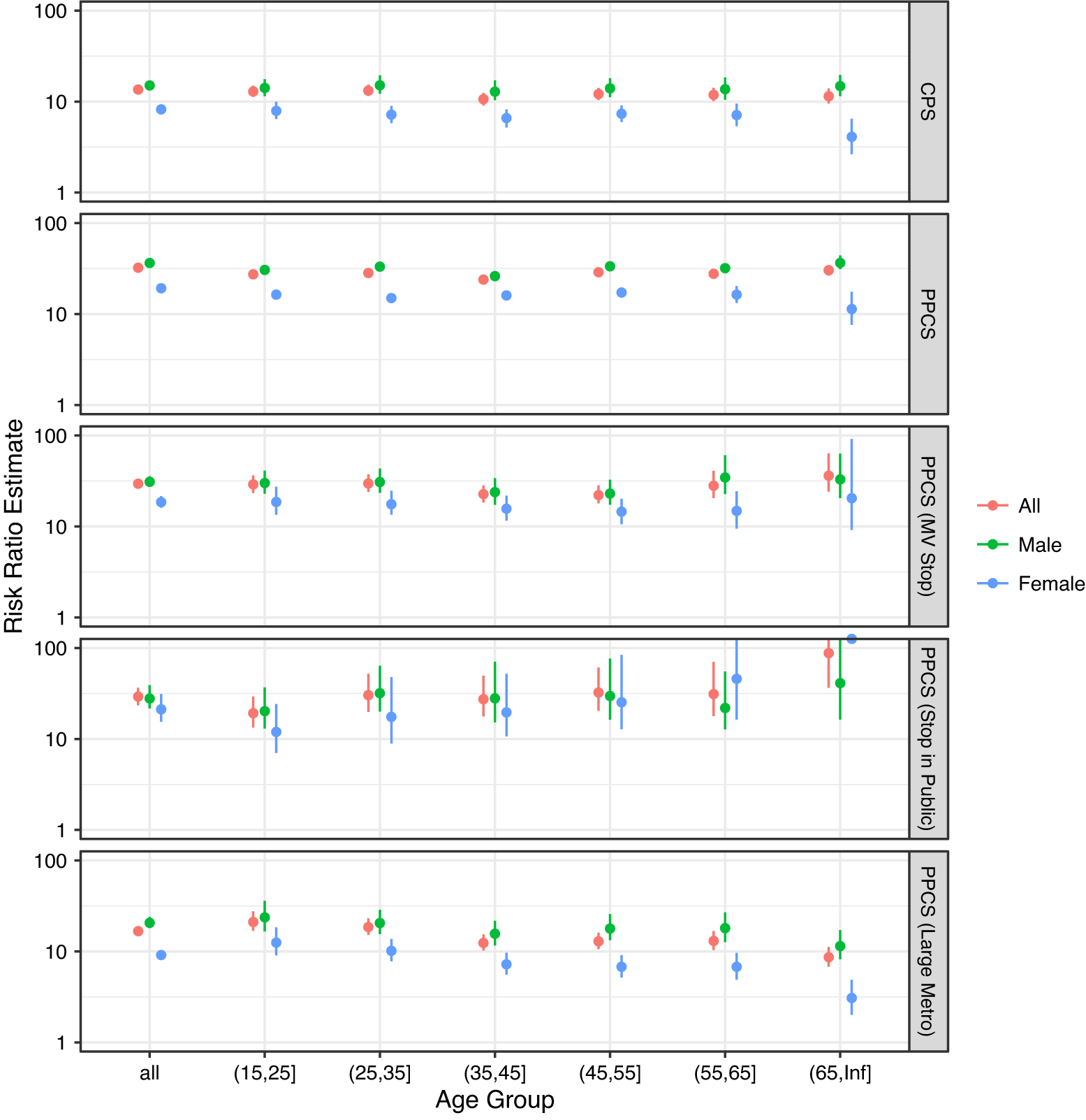
Figure D.1. Results of the Stratified Analysis of the NYPD Stop-and-Frisk Dataset by Age and Gender. The Estimated Risk Ratio Is Truncated at 100


 Open access
Comments
No Comments have been published for this article.