


1. Details of software download and set-up
DivFolio is an open public domain freely available software application developed in R Shiny environment for supporting wealth management in green finance. All materials and brief instructions are deployed on the GitHub repository:
https://github.com/QuantFILab/Divfolio.
Users can access the tool via three optional ways: web application, executable package, and running on RStudio.
Web Application
Web applications are the simplest way to access the tool online. Users are not required to install the application to a local machine. It only require an internet connection to utilize the tool. It was deployed on the shinyapps.io, an open source deployment sever provided by RStudio. The tool can be assessed via the URL:
https://quantfilab.shinyapps.io/divfolioserveri/
Note here that some features are limited due to processing capability of the deployment server. The details are given in Appendix A.2. For complete set of features, users can run the executable package locally on their computer or compile the github provided code, as described in the next section.
Executable Package
The executable package can be installed on Windows machines, Windows emulators on Mac, and Linux on the GitHub repository. It can be accessed on GitHub, https://github.com/QuantFILab/Divfolio, by downloading the folder name “ExecutablePackage” to the local machine and then doubly click on the Divfolio.exe to run the tool. It may take a long time to open the application in the first time. Unlike the web application mode, the executable package only requires an internet connection during installation. Once installed on the local machine, the users can utilize the tool without an internet connection. The executable file is self-contained, and it is not required to have an R environment installed to run the code. The file’s size is very large (1Gb), so it is advisable to download it on a network connection for faster file download. For an optimal user experience, it is highly recommended to follow the instructions provided on the GitHub repository for setting up and running the executable file. Note that the construction of the executable file utilised an R packaged called “electron-packer,” which we have unit tested and found it demonstrated satisfactory performance in our tests on Windows 10 operating system; however, we cannot vouch for comparable reliability on all possible operating systems. Given these constraints, and to prevent potential inconveniences, we suggest that if users find the executable is not configured to work with their operating system, they should revert to using DivFolio either via the Web application or running the source code from RStudio environment (or any IDE for R as outlined below).
Running from RStudio
Users who already have R installed may also run the Shiny application directly within an R environment that matches the specified user requirements as provided on the GitHub repository and in the readme file of the tool where required dependencies are listed. This option is suitable for R users. R and RStudio are required to be installed. In addition, the package “shiny” need to be called in R code. The code is simply:
library(shiny)
shiny::runGitHub("QuantFILab/Divfolio")
This option may be problematic when the package and R version do not match the code. Based on the most recent update, Version 4.2.2 or later of R is suggested. On GitHub, the most recent version of the packages and their dependencies can be found.
2. Introduction to DivFolio application
The main purpose of the software (DivFolio) is to support the development and assessment of portfolios that consider decarbonization and Environmental Social Governance (ESG) investing and divestment practices following the climate change prevention trends arising in wealth management practices. The software offers functionality for generating divestment plans and sustainable portfolios as well as for comparing the corresponding risk/return profiles, ESG scores, and customized attributes of portfolios, such as carbon intensity. The assessment is based on simulations that collect and incorporate relevant historical market data before and after divestment while also considering varying rates of divestment planning. The software allows the user to apply these assessments to publicly traded equity assets, exchange-traded funds (ETFs), exchange-traded notes (ETNs), and depositary receipts (DR).
Climate change has become a permanent long-term systemic risk. Regulators, consumers, and investors are becoming increasingly concerned about sustainability, which is driving a paradigm shift in investment and wealth management practices; see Fang et al. (Reference Fang, Tan and Wirjanto2019), Focardi & Fabozzi (Reference Focardi and Fabozzi2020), Benedetti et al. (Reference Benedetti, Biffis, Chatzimichalakis, Fedele and Simm2021), Tokat-Acikel et al. (Reference Tokat-Acikel, Aiolfi, Johnson, Hall and Jin2021) and Marupanthorn et al. (Reference Marupanthorn, Nikitopoulos, Ofosu-Hene, Peters and Richards2022). At a macroeconomic level, the majority of G10 countries and United Nations member states are increasingly focusing on developing targets and strategies to incentivise the transition toward a low carbon economy globally via frameworks such as the Sustainable Development Goals (SDGs)Footnote 1 and the 2030 Agenda (Miralles-Quirós & Miralles-Quirós, Reference Miralles-Quirós and Miralles-Quirós2021). The resultant actions involve mixed strategies, including both direct actions in terms of cutting emissions and moving away from fossil fuel-intensive industry and power generation, but also indirect actions such as incentivizing changes in investment practices. This manuscript focuses on these indirect actions related to wealth management and investment practices that try to align capital deployment with a green finance framework in order to reward commercial entities actively engaging in aligning with the United Nations SDGs. These practices also seek to achieve optimal target scores on ratings, such as the ESG scoring systems, which many financial rating agencies are actively developing, see Pagano et al. (Reference Pagano, Sinclair and Yang2018). The current ESG scores are in their infancy, which brings a lack of alignment in ESG scoring and rating methodology (Dimson et al., Reference Dimson, Marsh and Staunton2020). Nevertheless, such methods will mature and standardize and eventually become the metrics by which investors will evaluate corporate activities when it comes to environmental perspectives and actions. It is important to understand how this can influence and consequently affect portfolio and wealth management performance, as all listed companies in most major economies are now being actively rated for ESG criteria. This places expectations on the companies to achieve adequate ratings to satisfy increasing numbers of environmentally focused investment practices both in the retail markets and the wealth management population.
These changing perspectives on how to monitor, track, and analyze actions aiming to mitigate the effects of climate change are being encoded in various ways. For example, via the ESG scoring frameworks being developed in the financial investment space or via the development of the notion of carbon footprints of investment portfolios, see examples in Boermans & Galema (Reference Boermans and Galema2019) and Boermans et al. (Reference Boermans and Galema2017) who studied carbon footprints of large pension funds. In the asset management space, there is an ongoing debate about how to best incentivize corporations in order to foster private sector initiatives that will actively create a paradigm shift in decision-making toward more sustainable and environmentally friendly corporate decisions, eventually leading to a reduction in environmental impact. Such movements in investment practice are critical indirect drivers of change as they generate active decision-making that eventually leads to mitigation strategies that reduce carbon emissions, a primary driver of climate change. Even though there are many alternative approaches to achieve these strategic changes, including engagement, this manuscript and the proposed software consider the concept of “fossil-fuel divestment strategies”. Investors and asset managers are increasingly interested in optimal divestment strategies of their holdings from companies that either produce large amounts of carbon as part of their primary business models, such as fossil fuel companies in the energy sector, or companies classified as non-compliant or performing poorly on the environmental component of ESG ratings. For most institutional investors, such as pension funds (Rempel & Gupta, Reference Rempel and Gupta2020) and mutual funds (Guo et al., Reference Guo, Liang, Umar and Mirza2022), divestment is sometimes expensive without careful long-term planning, and on fund management expense (Marupanthorn et al., Reference Marupanthorn, Nikitopoulos, Ofosu-Hene, Peters and Richards2022). Mechanisms to develop, study, and analyze various divestment strategies are an essential component of carbon reduction strategies, while the rate at which investors should divest has become a critical aspect of effective divestment (Marupanthorn et al., Reference Marupanthorn, Nikitopoulos, Ofosu-Hene, Peters and Richards2022). In this manuscript, we present a software application that provides a comprehensive approach to analyze asset allocation methodologies to address and assess this impact over time on global equity portfolios and ETFs.
DivFolio is a public domain free software that acts as a digital platform constructed as an R Shiny application that users can utilize at their own risk as a decision-making tool on optimal divestment strategies based on historical data. The application embeds both manual and automatic options. Users can study a variety of divestment strategies, either by manually selecting their preferred stocks to invest/divest from or by utilizing the software to automatically select divestment assets based on quantiles of ESG scores. Users would be only required to select a proportion of divestment positions. The software uses the multiperiod optimization, i.e., time-dependent portfolio optimization, divestment frameworks proposed in Marupanthorn et al. (Reference Marupanthorn, Nikitopoulos, Ofosu-Hene, Peters and Richards2022). Note that these divestment strategies are designed for static-asset portfolio allocations, i.e., the investor does not aim to add new assets during divestment. The R Shiny application allows the user to select from globally listed equity assets, ETFs, and ETNs and to select these in both investment and divestment categories based on criteria such as ESG rankings, performance, and carbon emissions. The software interface also provides a variety of sets of multiperiod portfolio risk, return, and ESG-based analytics to explore the effects of divestment practices related to ESG and carbon footprints on different divestment and rate of divestment choices.
DivFolio allows users to compare the risk/return profiles, ESG scores, and customized attributes of portfolios (before and after divestment) based on the simulation using historical data. Furthermore, advanced options are considered, such as the assessment of portfolio stability via clustering and Graphical Lasso-based diversification assessment of correlation structures. The tool is also useful for investigating the impact of divestment on portfolio performance in multidimensional views of risk/return of the portfolio over time, the portfolio stability in risk/return profile, and the diversification structure in the portfolio, as divestment unfolds over time. DivFolio also affords the user the benefits of a general-purpose portfolio performance comparison, especially in ESG investing and sustainable investing. Furthermore, users can customize the attributes of comparable portfolios by uploading prepared comma-separated values (CSV) files on the tool instead of generating portfolios in order to compare their existing portfolio positions to those automatically generated by the scenarios users select in the DivFolio application.
The aim of the paper is to present the DivFolio software, explain its functionality, and demonstrate its applicability. Therefore, the paper should be treated as a guideline manual for users. Given that this is a software paper, we focus on presenting and explaining the software and do not attempt to provide a detailed account of the financial interpretations of the associated divestment strategies. For the financial interpretations and implications of findings on divestment strategies, we refer users to the empirical study Marupanthorn et al. (Reference Marupanthorn, Nikitopoulos, Ofosu-Hene, Peters and Richards2022) that presents the multiperiod optimization divestment frameworks built in DivFolio. Note that study, Marupanthorn et al. (Reference Marupanthorn, Nikitopoulos, Ofosu-Hene, Peters and Richards2022) does not provide a description of DivFolio, even though DivFolio has been used to carry out the empirical analysis of the study. Furthermore, the case studies considered in this paper for demonstration purposes and the case studies investigated in Marupanthorn et al. (Reference Marupanthorn, Nikitopoulos, Ofosu-Hene, Peters and Richards2022) are different to ensure novelty.
The remaining of this paper is arranged as follows. Section 3 explains the methodologies and algorithms embedded in the software. Section 4 presents illustrative examples on environmental score assets divestment in the energy and utility sectors and overall ESG score assets divestment in FTSE100. Section 5 presents an application of DivFolio to evaluate the impact of divestment on the risks and return of mixed pension portfolios using environmental risk score analysis. Section 6 concludes. The guidelines on how to use DivFolio are presented in Appendix A.
3. Overview of the methodology in the DivFolio application
The divestment methodology underpinning the DivFolio application and the corresponding mathematical frameworks are detailed in Marupanthorn et al. (Reference Marupanthorn, Nikitopoulos, Ofosu-Hene, Peters and Richards2022). Accordingly, we keep this section brief and refer the interested reader to the aforementioned paper for details.
3.1. DivFolio: multiperiod optimal portfolio selection with divestment
The three sequential processes used in DivFolio are summarized below.
Process 1: Generation of core portfolios
DivFolio offers five core portfolio choices. The Passive Equal-Weighted Portfolio (PEW) is a buy-and-hold portfolio with a passive investment long-only structure that provides a long-term investment strategy. The weights of all assets are fixed and do not fluctuate over time, i.e., $w_i = 1/N$
for
$w_i = 1/N$
for $i$
in the universe of
$i$
in the universe of $N$
assets, and short positions are forbidden. The Active Equal-Weighted Portfolio (AEW) is a portfolio in which the weights are balanced to achieve relative equal weighting. In other words, it is a return-weighted portfolio whose objective is to achieve the same return from each asset. The Global Minimum Variance Portfolio (GMV) tries to diversify assets with the lowest portfolio risk, as assessed by portfolio variance (Markowitz, Reference Markowitz1968; Markowitz, Reference Markowitz1952). In the case of the GMV portfolio, the optimal weights to invest for each asset are determined using the classical optimization problem that minimizes the variance of the portfolio’s return according to the Mean-Variance Markowitz framework as follows:
$N$
assets, and short positions are forbidden. The Active Equal-Weighted Portfolio (AEW) is a portfolio in which the weights are balanced to achieve relative equal weighting. In other words, it is a return-weighted portfolio whose objective is to achieve the same return from each asset. The Global Minimum Variance Portfolio (GMV) tries to diversify assets with the lowest portfolio risk, as assessed by portfolio variance (Markowitz, Reference Markowitz1968; Markowitz, Reference Markowitz1952). In the case of the GMV portfolio, the optimal weights to invest for each asset are determined using the classical optimization problem that minimizes the variance of the portfolio’s return according to the Mean-Variance Markowitz framework as follows:
 \begin{equation} \min _{{w}} \ \frac{1}{2}{w\Sigma w^T} \ \ \text{s.t.} \ \ {w1} = 1, \end{equation}
where $\Sigma$
is the covariance matrix of the asset returns,
$\Sigma$
is the covariance matrix of the asset returns, $w$
is the vector of the asset weights, and
$w$
is the vector of the asset weights, and $1$
is the column vector of ones. The Maximum Sharpe Ratio Portfolio (MS) is a portfolio that aims to achieve the maximum risk-adjusted return. The optimization problem assigns weights so as to maximize the Sharpe ratio of the portfolio (Sharpe, Reference Sharpe1966). The MS’s optimization is given as the solution to the classical Mean-Variance Markowitz framework as follows:
$1$
is the column vector of ones. The Maximum Sharpe Ratio Portfolio (MS) is a portfolio that aims to achieve the maximum risk-adjusted return. The optimization problem assigns weights so as to maximize the Sharpe ratio of the portfolio (Sharpe, Reference Sharpe1966). The MS’s optimization is given as the solution to the classical Mean-Variance Markowitz framework as follows:
 \begin{equation} \max _{{w}} \ {w}^T\mu - \frac{1}{2}{w\Sigma w^T} \ \ \text{s.t.} \ \ {w1} = 1, \end{equation}
where $\mu$
is the expected return of the portfolio assets. DivFolio also provides a set of portfolio strategies based on risk factor decompositions using the Principal Portfolios (PC) framework. This is created through a convex combination of the sub-portfolios generated by each principal component of the assets covariance matrix, with the convex weight coefficient determined by the eigenvalues,
$\mu$
is the expected return of the portfolio assets. DivFolio also provides a set of portfolio strategies based on risk factor decompositions using the Principal Portfolios (PC) framework. This is created through a convex combination of the sub-portfolios generated by each principal component of the assets covariance matrix, with the convex weight coefficient determined by the eigenvalues,
 \begin{equation} R_{PC} = \sum _{k = 1}^d \widetilde{\lambda }_k \sum _{i = 1}^N v_{i,k} R_i, \end{equation}
where $i$
is an index of the asset in universe with
$i$
is an index of the asset in universe with $N$
assets and
$N$
assets and $k$
is an index of the principal component with
$k$
is an index of the principal component with $d$
outstanding principal components such that
$d$
outstanding principal components such that $ 0 \leq d \leq N$
,
$ 0 \leq d \leq N$
, $\widetilde{\lambda }_k$
is a normalized eigenvalue of the principal component
$\widetilde{\lambda }_k$
is a normalized eigenvalue of the principal component $k$
such that
$k$
such that $\sum _{k = 1}^d \widetilde{\lambda }_k$
= 1, and
$\sum _{k = 1}^d \widetilde{\lambda }_k$
= 1, and $v_{ik}$
is the coordinate of the principal component
$v_{ik}$
is the coordinate of the principal component $k$
of asset
$k$
of asset $i$
(Yang, Reference Yang2015). The improved version of the PC with minimum variance is used in the application.Footnote 2
$i$
(Yang, Reference Yang2015). The improved version of the PC with minimum variance is used in the application.Footnote 2
DivFolio allows the user to consider both short and long positions (which are permitted in portfolio formation), except for the strategies of PEW and AEW portfolios, which restrict short positions. However, to avoid excessive leverage in the portfolio that arises when unrestricted short positions are admissible, we impose a “box” constraint to mitigate excess leverage. We introduce the box constraint in the multiperiod portfolio optimization by re-normalizing asset weights incrementally. These constraints are as follows:
 \begin{equation} w^s_{box} = \begin{cases} SL\times (w^s/\sum _{s \in S}{w^s}), & \ \sum _s w^s \gt SL, \\ w^s, & \sum _s w^s \leq SL, \end{cases} \end{equation}
where $S$
is the collection of assets that is taking short positions, and the weight
$S$
is the collection of assets that is taking short positions, and the weight $w^s$
indicates the size of the short position for an asset from set
$w^s$
indicates the size of the short position for an asset from set $S$
. The total leverage on the short positions is capped at level
$S$
. The total leverage on the short positions is capped at level $SL$
. Therefore, there are
$SL$
. Therefore, there are $N-|S|$
assets making up the subset of long positions, denoted by set
$N-|S|$
assets making up the subset of long positions, denoted by set $L$
, each having long positions of weight
$L$
, each having long positions of weight $w^l$
. Next, a sum of long positions is normalized to be
$w^l$
. Next, a sum of long positions is normalized to be $1 + SL$
if the short ratio exceeds the limit as detailed below:
$1 + SL$
if the short ratio exceeds the limit as detailed below:
 \begin{equation} w^l_{box} = \begin{cases} (1+SL)\times (w^l/\sum _{l \in L}{w^l}), & \ \sum _l w^l \gt SL, \\ w^l, & \sum _l w^l \leq SL. \end{cases} \end{equation}
This ensures that the portfolio limits excess leverage according to the user-defined or regulation-defined restrictions on long-short equity funds in asset management.
Process 2: Divestment controlled by a user-specified divestment schedule
Mathematically, the divestment schedule is an extra restriction imposed by the portfolio optimization problem over multiple time periods corresponding to the user’s selected divestment time horizon. In addition, it represents a multiperiod problem since the divestment schedule, $D(t)$
, is time-dependent. As a guide to the user, DivFolio offers three (simple) functional rates of divestment, including, for instance, linear and hyperbolic decaying. The user can select parameters for these different divestment schedules, the start and end periods, and the set of assets to divest from. In the case of instant divestment, the controlling equation is denoted by
$D(t)$
, is time-dependent. As a guide to the user, DivFolio offers three (simple) functional rates of divestment, including, for instance, linear and hyperbolic decaying. The user can select parameters for these different divestment schedules, the start and end periods, and the set of assets to divest from. In the case of instant divestment, the controlling equation is denoted by
 \begin{equation} D(t) = 0, \end{equation}
for all $t$
, where
$t$
, where $D(t)$
is the divestment schedule at time
$D(t)$
is the divestment schedule at time $t$
. The linear rate gradually withdraws divestable assets by the equal capital reduction of
$t$
. The linear rate gradually withdraws divestable assets by the equal capital reduction of $m$
each time step. The governing equation is given by
$m$
each time step. The governing equation is given by
 \begin{equation} D(t) = m \times (t -t_{end}), \end{equation}
where $t_{end}$
is the index of the last date of divestment. Finally, the hyperbolic rate allows to withdraw divestable assets more rapidly in the early time step, based on a hyperbolic decaying function with exponent
$t_{end}$
is the index of the last date of divestment. Finally, the hyperbolic rate allows to withdraw divestable assets more rapidly in the early time step, based on a hyperbolic decaying function with exponent $a$
that is user-defined. The governing equation is given by
$a$
that is user-defined. The governing equation is given by
 \begin{equation} D(t) = 1/t^a, \end{equation}
where $a$
is the non-negative exponent. The end date of divestment is the last date of divestment. After this date, the sum of the weights of all divestable assets is set to zero.
$a$
is the non-negative exponent. The end date of divestment is the last date of divestment. After this date, the sum of the weights of all divestable assets is set to zero.
The resulting portfolio optimization problem is then a multiperiod problem with a functional constraint over time, which is approximated via a sequence of locally constrained portfolio optimization problems. This is very important for practical reasons related to the speed at which results are produced by the application. The performance of this approximation in large portfolios with 500+ assets is assessed in Marupanthorn et al. (Reference Marupanthorn, Nikitopoulos, Ofosu-Hene, Peters and Richards2022). It is shown that, relative to slower numerical solvers, the approximation has acceptable accuracy and significantly speeds up the solution attainment.
To approximate the multiperiod problem, we separate the optimization into two subproblems: divestment and reinvestment. The process is applied when the portfolio is rebalanced. Let $L$
and
$L$
and $S$
be the sets of indices of the long-position and short-position assets, and the superscript
$S$
be the sets of indices of the long-position and short-position assets, and the superscript $\cdot ^{div}$
indicates the divestable assets. In the divestment stage, if the sum of the weight of the divestable assets hits or exceeds the divestment schedule
$\cdot ^{div}$
indicates the divestable assets. In the divestment stage, if the sum of the weight of the divestable assets hits or exceeds the divestment schedule $D(t)$
,
$D(t)$
, $\sum _{l \in L}w^{l,div}_{box} \geq D(t)$
, or/and,
$\sum _{l \in L}w^{l,div}_{box} \geq D(t)$
, or/and, $\sum _{s \in S}w^{s,div}_{box} \leq -D(t)$
, then it is scaled in the bound as follows:
$\sum _{s \in S}w^{s,div}_{box} \leq -D(t)$
, then it is scaled in the bound as follows:
 \begin{equation} \widetilde{w}^{l,div}= D(t) \times \frac{w^{l,div}_{box}}{\sum _{l \in L}w^{l,div}_{box}}, \quad \text{or/and} \quad \widetilde{w}^{s,div} = -D(t) \times \frac{w^{s,div}_{box}}{\sum _{s \in S}w^{s,div}_{box}}. \end{equation}
Otherwise, we keep the weights without scaling, e.g., $\widetilde{w}^{s,div} = w^{s,div}_{box}$
, or/and,
$\widetilde{w}^{s,div} = w^{s,div}_{box}$
, or/and, $\widetilde{w}^{l,div} = w^{l,div}_{box}$
.
$\widetilde{w}^{l,div} = w^{l,div}_{box}$
.
Process 3: Reinvestment of excess investment weight
The reinvestment stage is to reallocate the capital, called the excess weights, from the divestable assets to the investable assets. The excess weights are allocated to the assets according to their proportion in the portfolio such that the assets with larger position sizes, i.e., larger weights gain more than those with lower portfolio weightings. The excess weights are defined by
 \begin{equation} w_{ex} = \begin{cases} \sum _{l \in L}\widetilde{w}^{l,div}_{box} - D(t), & \text{if} \ \sum _{l \in L}w^{l,d}_{box} \geq D(t), \\[4pt] \sum _{s \in S}w^{s,div}_{box} + D(t), & \text{if} \ \sum _{s \in S}w^{s,div}_{box} \leq -D(t), \\[4pt] \sum _{l \in L}w^{l,div}_{box} + \sum _{s \in S}w^{s,div}_{box}, & \text{if} \ \sum _{l \in L}w^{l,div}_{box} \geq D(t), \ \text{and} \ \sum _{s \in S}w^{s,div}_{box} \leq -D(t), \\[4pt] 0, & \text{otherwise}. \end{cases} \end{equation}
Then the new weight of the investable assets in the divested portfolio is calculated by
 \begin{equation} \widetilde{w}^{inv} = w^{inv} + \frac{w^{inv}}{\sum _{l \in L}w^{inv}} \times w_{ex}. \end{equation}
The obtained weight satisfies the normalizing condition, ${\widetilde{w}}^{l,div}{1} +{\widetilde{w}}^{s,div}{1} +{\widetilde{w}}^{inv}{1} = 1$
, where the superscript
${\widetilde{w}}^{l,div}{1} +{\widetilde{w}}^{s,div}{1} +{\widetilde{w}}^{inv}{1} = 1$
, where the superscript $\cdot ^{inv}$
indicates the investable assets.
$\cdot ^{inv}$
indicates the investable assets.
3.2. DivFolio: portfolio stability analysis by dynamic risk and return feature clustering using CLARA
DivFolio also collects throughout the multiperiod investment/divestment timeline, as selected by the user, a collection of portfolio risk measures and performance measures which act as feature vectors in period-by-period clustering analysis. This allows DivFolio to assess whether large changes in portfolio behavior are observed relative to non-divestment strategies as a result of different divestment strategies. It also forms a type of risk and performance-sensitive stability assessment for the portfolio strategies and divestment strategies as selected by the user.
Portfolio stability refers to the similarity of the relative movement of an attribute, such as return, volatility, VaR, drawdown etc., across a collection of portfolios over time. When one starts to impose divestment strategies of various forms within a given portfolio strategy, this reduces the possible universe of investable assets increasingly over time. This can affect risk and return profiles for the performance of the strategy relative to the same strategy without such restrictions. DivFolio provides valuable feedback in this regard by mapping which user-defined components of strategy and divestment set selection and divestment rate is most likely to cause instability in risk/return profiles. Therefore, users can seek outcomes that may minimise such effects in their investment decisions.
Producing results in a timely manner for DivFolio users is achieved using a machine learning unsupervised clustering technique based on the feature vectors for daily portfolio performance within each rebalancing period (using a default 30-day rebalancing window). As proposed in Kaufman & Rousseeuw (Reference Kaufman and Rousseeuw2009), Clustering Large Applications (CLARA) is utilized by DivFolio to group the following risk-return characteristics: return, volatility, Sharpe ratio, maximum drawdown, Sortino ratio, cumulative return, and value at risk into daily feature vectors for clustering for any given portfolio strategy. The risk profiles of each portfolio are presented as time series. CLARA is applied multiple times during distinct time frames. The performance of portfolios belonging to the same cluster is comparable and not significantly different, implying stability of the risk profiles of portfolios over time.
The algorithm for CLARA implemented in DivFolio is summarized in pseudo-code in the guide in the associated GitHub repository. CLARA is designed to pull numerous samples from the dataset, apply partitioning around medoids algorithm (PAM) to each sample, identify the medoids, and then return the optimal grouping. The PAM algorithm is then applied to $D'$
to identify the
$D'$
to identify the $k$
medoids, calculate the current dissimilarity utilizing these
$k$
medoids, calculate the current dissimilarity utilizing these $k$
medoids and the dataset
$k$
medoids and the dataset $D$
. If it is smaller than the previous iteration’s result, these
$D$
. If it is smaller than the previous iteration’s result, these $k$
medoids are retained as the optimal
$k$
medoids are retained as the optimal $k$
medoids. The entire procedure is repeated a predetermined number of times.
$k$
medoids. The entire procedure is repeated a predetermined number of times. $S$
is the subset index, and
$S$
is the subset index, and $Q$
and
$Q$
and $q$
are arbitrarily large values such that
$q$
are arbitrarily large values such that $Q \gt q$
initially.
$Q \gt q$
initially.
3.3. DivFolio: diversification profile of portfolios under divestment via Graphical Lasso regularization
Different portfolio constructions and divestment strategies (selection of divestment assets, rate of divestment, and timeline of divestment) may affect the diversification of portfolios over time. DivFolio includes a visual graph-based interface that allows users to assess these effects by plotting the evolution of the most significant (positive or negative) portfolio correlation relationships as the portfolio is progressively rebalanced over time, and the divestment assets are progressively removed from the portfolio.
This assessment is performed by using a robust covariance shrinkage technique. Graphical least absolute shrinkage and selection operator (glasso) Zhao et al. (Reference Zhao, Liu, Roeder, Lafferty and Wasserman2012) is suitable for studying the strongest/most robust dynamic correlation structure within a portfolio over time. From graphs of the correlation relationships over time within a portfolio undergoing divestment, one can learn about the influence that divestment may have on aspects of portfolio diversification. The glasso problem aims to find the best sparse and robust estimate covariance matrix under regularization. Mathematically, the optimization of the glasso considers the sparse Gaussian graphical model (Meinshausen & Bühlmann, Reference Meinshausen and Bühlmann2006) with the following minimization problem,
 \begin{equation} \hat{G} = \mathop{\textrm{arg min}}\limits_{G \in CG}{\frac{1}{2}\text{Tr}(G^TSG) - \text{Tr}(G^TS) + \lambda \lVert G \lVert _1}, \end{equation}
where $CG = \{G \in \mathbb{R}^{N \times N} | G_{i,i} = 0 \ \ \text{for} \ i = 1,\dots,N\}$
is a set of estimate sparse covariance matrix,
$CG = \{G \in \mathbb{R}^{N \times N} | G_{i,i} = 0 \ \ \text{for} \ i = 1,\dots,N\}$
is a set of estimate sparse covariance matrix, $\hat{G}$
is the best sparse estimate covariance matrix,
$\hat{G}$
is the best sparse estimate covariance matrix, $S$
is a simple covariance matrix, and
$S$
is a simple covariance matrix, and $\lambda$
is a positive regularization parameter governing the sparsity level. The optimization is analogous to fitting lasso to each variable using the other variables as predictions.
$\lambda$
is a positive regularization parameter governing the sparsity level. The optimization is analogous to fitting lasso to each variable using the other variables as predictions.
The strength of the correlation structure of the portfolio positions in assets can be investigated using glasso. The correlations of the assets in $\hat{G}$
that survive after regularization, i.e., the ones that remain nonzero after regularization, are the strongest relationships in the portfolio and have the strongest effects on diversification. DivFolio identifies these at each stage of rebalancing and divestment and provides a visual tool to explore these over time, allowing for the multiple comparisons of different portfolio strategies and divestment decisions. Thus, the application provides a powerful visual aid to capture the impact of investment decisions on portfolio diversification profiles over time in complex portfolio selections.
$\hat{G}$
that survive after regularization, i.e., the ones that remain nonzero after regularization, are the strongest relationships in the portfolio and have the strongest effects on diversification. DivFolio identifies these at each stage of rebalancing and divestment and provides a visual tool to explore these over time, allowing for the multiple comparisons of different portfolio strategies and divestment decisions. Thus, the application provides a powerful visual aid to capture the impact of investment decisions on portfolio diversification profiles over time in complex portfolio selections.
4. Illustrative example: divestment of a portfolio of UK stocks using DivFolio
We consider next an illustrative example based on a small portfolio of FTSE100 stocks from the Health Care, Energy, and Utilities sectors. We employ DivFolio to investigate the impact of a linear divestment schedule and assess performance in terms of improving the environmental score and affecting the risk profiles and other attributes over time. The asset universe consists of the following tickers: AZN.L, BP.L, DCC.L, GSK.L, HIK.L, NG.L, SHEL.L, SN.L, SSE.L, SVT.L, and UU.L, and the duration of the divestment is from January 2020 to December 2020. We select a set of assets from the Energy and Utilities sectors to be divested from based on their environmental scores being lower relative to Health Care sector assets. Divesting in this manner would improve the portfolio’s environmental rating. However, the divestment may drastically alter the risk profile or other characteristics of the divested portfolio relative to the original portfolio. All files used in this illustration can be found on our GitHub.
4.1. Guidelines of using DivFolio for the illustrative example
The input of the data for this example is detailed in the step-by-step visual aid in Figs. B.1–B.5 presented in the Appendix, with the optional tool components being illustrated in Figs. B.6–B.8. In each illustration, users are also shown the required format data files, if the manual upload is preferred, see for further details at our Github.
In Step 1, we enter a ticker into the software, for instance, the AstraZeneca PLC ticker, namely AZN.L. See an example of the DivFolio GUI in Fig. 1 for the corresponding collected foundation data, sustainability scores, candlestick chart of the asset’s price, and risk profiles for different time periods in Step 1. Next, each asset in the universe is added to the box in the Cart icon’s dropdown. The selected tickers are initially displayed in the Potential Assets box in Step 2. Next, we assign the investment status of the possible assets by dragging and dropping them into the Investable Assets or Divestable Assets boxes. The assets in Energy and Utilities sectors are dropped in the area of divestable assets, while the assets in Health care sector are dropped in the area of investable assets. We submit the assets list to receive the ESG scores by clicking the summary button. The data will be displayed on the table of attributes; see Fig. 2. The table should be saved as file F1 to avoid calling data from the server. To receive the returns in Step 3, we enter the initial date, 2020-01-03, and the final date, 2020-12-31, into the corresponding boxes in the Calendar icon’s dropdown menu. Then we click the Submit button. This table can be locally stored as an F2 file. Steps 1 to 3 are now complete in the sequential component.

Figure 1 Screenshots of the sustainability score, the candlesticks of historical data, and the bar chart of risk profiles in various time windows in Step 1.

Figure 2 Screenshots of the drag and drop menus: potential assets, investable assets and divestable assets, and the table of attributes in Step 2.

Figure 3 Screenshots of the table of rebalancing portfolio weight, the time series of asset weight, assets allocation, and the allocation of attributes in the portfolio in Step 4.

Figure 4 Screenshots of the distribution of attributes for long positions, the distribution of attributes for short positions, the distribution of portfolio risk profiles, and the efficiency frontier in Step 4. Screenshots of the distribution of the percentage of relative change between non-divested and divested portfolios in Step 5.

Figure 5 Screenshots of the table of divestment schedule, the portfolio weight after divestment, the sum of weights of divestable assets, the sum of allocated weights and investable assets weights in Step 5.

Figure 6 Screenshots of the time series of asset weight, the assets allocation, the attribute allocation in the portfolio, the distribution of attributes for long positions, and the distribution of attributes for short position in Step 5.
We aim next to generate the global minimum variance portfolio with a short limit of 0.3 in Step 4; see Fig. 3. For pairs of assets with an extremely high linear correlation, only one should be selected if the portfolio is to undergo a mean-variance optimization. We navigate to the drop-down menu of the bars icon, pick global minimum variance, toggle limit short-selling weight, and enter 0.3 in the short-selling limit box. The portfolio is rebalanced typically monthly. Therefore, we set the option for rebalancing frequency and the number of days for computing weights to 20. The process may be time-consuming proportionally to the number of assets in the portfolio. Portfolio weights will be shown in the Table of rebalancing portfolio weight. This table is equivalent to the file F3. A selection of some of the outputs of DivFolio based on the steps described in previous sections is shown in Figs. 3 and 4. Note that the efficient frontier is only accessible for the portfolio created by DivFolio. The efficiency boundaries are formed by the backward lag return of $\tau$
days selected in Step 4, whereas the dots represent the expected return vs the risk of the portfolios whose weights were derived using the backward lag return of
$\tau$
days selected in Step 4, whereas the dots represent the expected return vs the risk of the portfolios whose weights were derived using the backward lag return of $\tau$
, but applied to the subsequent return window.
$\tau$
, but applied to the subsequent return window.
Further, we assume a linear rate of divestment with a slope $m = -0.1$
, by setting the end date at 2020-12-10. DivFolio’s generated divestment schedule is displayed, and the results of this stage are equivalent to file F4, which can be downloaded locally for future use. Fig. 5 displays examples of comparison outputs from DivFolio that illustrate differences between divested portfolio and the non-divested portfolio. The weight of the divestable assets reduces over time according to the divestment schedule. Step 5 that displays changes in the attributes over time are also examined in the panel of attribute allocation in the portfolio and their distribution in the plots of the distribution of attributes for long and short positions (see Fig. 6).
$m = -0.1$
, by setting the end date at 2020-12-10. DivFolio’s generated divestment schedule is displayed, and the results of this stage are equivalent to file F4, which can be downloaded locally for future use. Fig. 5 displays examples of comparison outputs from DivFolio that illustrate differences between divested portfolio and the non-divested portfolio. The weight of the divestable assets reduces over time according to the divestment schedule. Step 5 that displays changes in the attributes over time are also examined in the panel of attribute allocation in the portfolio and their distribution in the plots of the distribution of attributes for long and short positions (see Fig. 6).
4.2. Sequential assessment with DivFolio
We assess the divestment effect of the global minimum variance long-short portfolio (less than 30% in short weight) with a linear schedule for one year, from 2020-01-03 to 2020-12-31. We consider divesting holdings from the Energy and Utilities sectors and after completing the sequential process from Steps 1 to 5, we present an illustration of results obtained using DivFolio. Note that, it is beyond the purpose of this paper to demonstrate every aspect of the DivFolio software output. We only provide some illustrative selections of the results generated by the software. This illustration intends to demonstrate the tool’s outcomes and should not be considered a detailed case study. The interested reader in a such detailed analysis of financial portfolios and divestment strategies using DivFolio are referred to Marupanthorn et al. (Reference Marupanthorn, Nikitopoulos, Ofosu-Hene, Peters and Richards2022).
Fig. 1 demonstrates core attributes for each individual asset. These attributes help users with decisions about which assets are relatively weaker on ESG, E, S, or G scores compared to others, so they can make more informed decisions on portfolio divestment. In Fig. 1 demonstration, we see an example of the pharmaceutical company AstraZeneca PLC, its ESG, E, S, and G scores, as well as its share price, trading volume profiles, and a risk profile decomposition over multiple time scales for the individual asset.
In Fig. 2, the user has an interactive display of various sets of assets they may choose to invest or divest from. Note that the user also has a selection of predefined global indexes with a visual tool for selection by country, should they be exploring assets in various countries and wish to have automated asset population features. In this illustrative example, we have selected UK-listed equity assets (as indicated by the .L after the ticker). This figure demonstrates how easy it is to get a summary of the current portfolio decisions regarding assets to invest in and those to divest from over time.
Fig. 3 illustrates the types of results this stage of the DivFolio software provides the users. For instance, we see that for the user-selected portfolio investment set/divestment set of assets and user-selected portfolio strategy and divestment rate (set in Step 3) the output from Step 4 summarizes visuals of the performance of the portfolio over time. It displays each asset position weights in the portfolio, the sector weightings concentrated on in the portfolio over time for each asset, and long/short investment position total positions over time together with their portfolio weighted ESG, E, S, and G scores.
Furthermore, as shown in Fig. 5, users are provided with further information regarding the portfolio performance. For example, for each period of time when rebalancing is undertaken, they can see the risk-return plane efficient frontiers and where their portfolio sits in this regard, as divestment is performed. Furthermore, they observe the violin (box plot and density) plots of the risk measures for the portfolios daily performance for that rebalancing period and the portfolios views of the ESG, E, S, and G scores for comparable divested and non-divested portfolios. In this illustrative example, users are provided with a detailed breakdown of the ESG portfolio positions for the divested assets and contrast to the positions that otherwise would have been taken, had divestment not been applied, for the user-selected portfolio strategy, see Fig. 6.
In addition, users are provided with a detailed breakdown of the ESG scores for the portfolio, throughout the divestment process. It allows one to assess the effects of divestment choices. Fig. 6 also displays an illustrative example of the portfolio’s environmental score benefits from divestment. It is clear that over time, the divestment portfolio is improving in the E scores; however, this comes at the cost of worsening S and G scores for the portfolio. This is evident from both the sequential decomposition plots of the portfolio long and short ESG, E, S, and G scores over time, and the net results from the boxplots provided contrasting the non-divestment case with the divestment outcomes of the portfolio ESG score analysis. Hence, this example illustrates that the reinvestment in the Health care sector from funds divested from the Energy sector degrades performance in the total ESG score of the portfolio since the environmental score improvement is offset by the social and governance scores degrading.
The software also allows users to assess the portfolio risk measures, by providing a comprehensive risk assessment of the users’ portfolio strategy when combined with divestment choices. Fig. 6 illustrates a comparison of risk profiles that is very valuable for investors’ decision-making regarding divestment practices. For instance, this example demonstrates that divestment creates excess risk in all dimensions of the risk assessment. The larger body of the boxplot indicates greater profile variation. The mean and median of the risk profile distribution of the divested portfolio are also less favorable than those of the original portfolio, indicating that divestment in this case has made the portfolio riskier.
4.3. DivFolio’s advanced analytics Options I, II, and III
We next examine some examples of the types of results that users can obtain from the optional advanced analytics by DivFolio and demonstrate the functionality of the individual advanced analytics tools embedded in DivFolio, namely Options I, II, and III. Recall that these tools allow the comparison of multiple portfolios. To produce this illustrative example, we use File F5 from DivFolio in Step 5 containing the weights of four portfolios as of the rebalancing date. These portfolios include the original portfolio (PEW), the divested portfolio with a linear rate of divestment (Linear, $m = -0.1$
), the hyperbolic rate (Hyber,
$m = -0.1$
), the hyperbolic rate (Hyber, $a = 1.2$
), and the instant divestment (Instant). The names of the portfolios are listed in the ‘PORTNAME’ column. Note that, the file F2 is obtained from Step 1. Files F1 and F6 can be either used here as they contain the commonly required columns of “Ticker” and “Status”.
$a = 1.2$
), and the instant divestment (Instant). The names of the portfolios are listed in the ‘PORTNAME’ column. Note that, the file F2 is obtained from Step 1. Files F1 and F6 can be either used here as they contain the commonly required columns of “Ticker” and “Status”.
We conduct a performance comparison of these four portfolios by using Option I. Fig. 7 compares the relative weights of the divestable and the investable assets along with a plot of attribute allocation in a portfolio calculated by Eq. (A3). Fig. 8 compares the distribution of weighted attributes for the long position (there is no short position in the PEW) and the distribution of risk profiles. The distribution of attributes for PEW and instant rates is uniform, as their weights remain constant over time. Finally, the plots of the relative change in the percentage of each portfolio compared to the benchmark (PEW) are illustrated in Fig. 9.

Figure 7 Screenshots of the time series of assets weight, the sum of weights of divestable assets, the sum of weights allocated to investable assets and the attribute allocation in portfolio in Option I.

Figure 8 Screenshots of the distribution of attributes for a long position (left) and the distribution of risk profiles (right) in Option I.

Figure 9 Screenshots of the distribution of the percentage of relative change compared to benchmarks in Option I.
Option II contains the stability analysis results. The number of days in the time window, $\tau$
and the number of days used in cluster analysis,
$\tau$
and the number of days used in cluster analysis, $t$
, are both set to 20 days (monthly) for this illustration. Fig. 10 compares the aggregate risk profiles with the average of the previous 20 days. Distinctions between the benchmark, immediate, and hyperbolic rates of divestment are evident. Fig. 11 depicts the heatmaps of cluster labels utilizing CLARA for each risk profile. Since the beginning of the study period, the instant and hyperbolic divestment rates have produced stable portfolio performance throughout the study results, as their labels of the cluster have remained consistent over time, except for the Sharpe and Sortino ratios at the first rebalance.
$t$
, are both set to 20 days (monthly) for this illustration. Fig. 10 compares the aggregate risk profiles with the average of the previous 20 days. Distinctions between the benchmark, immediate, and hyperbolic rates of divestment are evident. Fig. 11 depicts the heatmaps of cluster labels utilizing CLARA for each risk profile. Since the beginning of the study period, the instant and hyperbolic divestment rates have produced stable portfolio performance throughout the study results, as their labels of the cluster have remained consistent over time, except for the Sharpe and Sortino ratios at the first rebalance.

Figure 10 Screenshots of the aggregate time series of risk profiles in Option II.

Figure 11 Screenshots of the clustering results in Option II.
In Fig. 12, Option III component analyzes the diversification profile of portfolios under divestment. The most persistent and strongest correlations between pairs of assets in the portfolio positions are extracted, in a graph format, where each vertex is a portfolio asset position over time and each edge is a strong correlation relationship between the portfolio sub-positions at this point in time. The figure contrasts the graph structure of correlation in Eq. (A6) in three-time steps of rebalancing: the second, ninth, and twelfth out of twelve times rebalancing. Over time, the weighted covariance of the portfolio’s assets decreases proportionally, as shown by fewer links than the initial rebalancing in all portfolios. The consistency of the graph structures during and after divestment suggests that, in this example, the allocation of investment weight from divestable assets to investable assets does not significantly impact the correlation relationships between the changing positions for pairs of assets over time.

Figure 12 Screenshots of the portfolio network structure of covariance in Option III.
5. Applying DivFolio to evaluate the impact of divestment on risk and return in mixed pension portfolios using environmental risk score analysis
Fully funded pension schemes designate specific reserves for members’ pensions and channel investments into assets such as equities and real estate to foster capital appreciation. While these schemes present distinct investment prospects and transparent valuation metrics, they are also susceptible to market volatilities and administrative expenses. Furthermore, unfunded schemes – often referred to as Pay-as-you-go systems – depend on contemporaneous contributions to meet pension obligations. These systems are inherently streamlined, cost-efficient, and insulated from market perturbations. However, they grapple with challenges stemming from demographic trends and legislative amendments. Aligning both funds using the mean-variance methodology can potentially fine-tune the equilibrium between risk and return, underscoring the rationale for the integration of funded pensions with their unfunded counterparts Dutta et al. (Reference Dutta, Kapur and Orszag2000).
In this section, we demonstrate the application of the DivFolio framework to evaluate the impact of divestment on the risk and return profile of mixed pension funds, integrating both funded and unfunded components within the mean-variance framework.
5.1. Mixed pension fund portfolio
We explore the interplay between risk and return in both fully funded and mixed funded-unfunded pension structures, referencing the work in Dutta et al. (Reference Dutta, Kapur and Orszag2000). Let $ r$
represents the return from the funded pension, and
$ r$
represents the return from the funded pension, and $ g$
the return from the unfunded pension. If
$ g$
the return from the unfunded pension. If $ w^f$
signifies the investment weight of the funded pension, then
$ w^f$
signifies the investment weight of the funded pension, then $ 1-w^f$
represents that of the unfunded pension. Given the portfolio dynamics of the mixed pension fund, the pension return is represented as
$ 1-w^f$
represents that of the unfunded pension. Given the portfolio dynamics of the mixed pension fund, the pension return is represented as
 \begin{equation} P = w^{f}r + (1-w^{f})g. \end{equation}
Adopting the minimum variance portfolio approach, our objective function becomes:
 \begin{equation} w^{f}_{\ast } = \mathrm{arg\,max}_{w^{f}} \quad \mathbb{E}(P) - \frac{\gamma }{2} \text{Var}(P), \end{equation}
where $ \gamma$
denotes the risk-aversion parameter. For cases where
$ \gamma$
denotes the risk-aversion parameter. For cases where $ \mu _r \gt \mu _g$
, an analytical solution is provided in Aaron (Reference Aaron1966):
$ \mu _r \gt \mu _g$
, an analytical solution is provided in Aaron (Reference Aaron1966):
 \begin{equation} w^{f}_{\ast } = \frac{\mu _r - \mu _g + \gamma (\sigma _g^2 - \sigma _{rg})}{\gamma (\sigma _{r}^2 + \sigma _{g}^2 - 2\sigma _{rg})}, \end{equation}
with $ \sigma _{rg}$
being the covariance between
$ \sigma _{rg}$
being the covariance between $ r$
and
$ r$
and $ g$
.
$ g$
.
5.2. Mixed pension fund divestment methodology
The mixed pension portfolio can be bifurcated into two distinct segments: the unfunded and the funded pension portfolios. Within our analytical paradigm, GDP growth serves as the representative metric for the returns of an unfunded pension, denoted as $ g_t$
. This choice is anchored in the methodology elucidated in Dutta et al. (Reference Dutta, Kapur and Orszag2000). The GDP growth rate at any given time can be expressed as
$ g_t$
. This choice is anchored in the methodology elucidated in Dutta et al. (Reference Dutta, Kapur and Orszag2000). The GDP growth rate at any given time can be expressed as
 \begin{equation} g_t = \frac{GDP_{t} - GDP_{t-1}}{GDP_{t-1}}. \end{equation}
Note that the divestment strategy is not applicable to the unfunded segment.
The funded pension portfolio is constructed using constituents from major national indices, specifically the S&P 500 for the United States and the FTSE 100 for the United Kingdom. To model this, we employ an equal-weighted portfolio strategy. Given a portfolio with $N$
constituents, the capital is evenly allocated across each asset, such that
$N$
constituents, the capital is evenly allocated across each asset, such that $w_{i} = \frac{1}{N}$
. The return of this non-divested portfolio can be formulated as
$w_{i} = \frac{1}{N}$
. The return of this non-divested portfolio can be formulated as
 \begin{equation} r_{t}^{\text{non-div}} = \sum _{i = 1}^N w_{i,t} r_{i,t} \end{equation}
where $w_{i,t} = \frac{1}{N}$
signifies the investment weight, and
$w_{i,t} = \frac{1}{N}$
signifies the investment weight, and $r_{i,t}$
represents the return of asset
$r_{i,t}$
represents the return of asset $i$
at time
$i$
at time $t$
. On the other hand, the return of the divested funded portfolio is defined as
$t$
. On the other hand, the return of the divested funded portfolio is defined as
 \begin{equation} r_{t}^{\text{div}} = \sum _{i = 1}^N w^{\text{div}}_{i,t} r_{i,t} \end{equation}
In this equation, $w^{\text{div}}_{i,t}$
is the investment weight that is constrained by the divestment schedule. This weight is determined by the divestment methodology outlined in Marupanthorn et al. (Reference Marupanthorn, Nikitopoulos, Ofosu-Hene, Peters and Richards2022) and can also be generated using the DivFolio tool.
$w^{\text{div}}_{i,t}$
is the investment weight that is constrained by the divestment schedule. This weight is determined by the divestment methodology outlined in Marupanthorn et al. (Reference Marupanthorn, Nikitopoulos, Ofosu-Hene, Peters and Richards2022) and can also be generated using the DivFolio tool.
Ultimately, the mixed pension portfolio is derived from the amalgamation of both the funded and unfunded portions. The return of the original portfolio, which does not incorporate any divestment, can be computed as
 \begin{equation} P_t^{\text{non-div}} = w^{f,\text{non-div}}_{\ast } r_{t}^{\text{non-div}} + \Big(1-w^{f,\text{non-div}}_{\ast }\Big) g_t, \end{equation}
where $w^{f,\text{non-div}}_{\ast }$
denotes the weight of the funded portion in the mixed pension portfolio for a non-divested portfolio,
$w^{f,\text{non-div}}_{\ast }$
denotes the weight of the funded portion in the mixed pension portfolio for a non-divested portfolio, $r_{t}^{\text{non-div}}$
is the return from the non-divested funded portfolio, and
$r_{t}^{\text{non-div}}$
is the return from the non-divested funded portfolio, and $g_t$
represents the GDP growth rate as previously defined.
$g_t$
represents the GDP growth rate as previously defined.
Similarly, the return for the divested mixed pension portfolio can be expressed as
 \begin{equation} P_t^{\text{div}} = w^{f,\text{div}}_{\ast } r_{t}^{\text{div}} + \Big(1-w^{f,\text{div}}_{\ast }\Big) g_t, \end{equation}
where $w^{f,\text{div}}_{\ast }$
is the weight of the funded portion in the mixed pension portfolio for a divested portfolio. The proposed formulation assumes that divestment strategies affect only the funded portion of the mixed pension portfolio, leaving the unfunded portion unchanged.
$w^{f,\text{div}}_{\ast }$
is the weight of the funded portion in the mixed pension portfolio for a divested portfolio. The proposed formulation assumes that divestment strategies affect only the funded portion of the mixed pension portfolio, leaving the unfunded portion unchanged.
5.3. Experimental design and data description
The primary objective of this case study is to discern the effects of divestment, informed by environmental scores, on the risk-return profile of mixed pension funds relative to their foundational investment strategies. Emphasizing assets that rank in the uppermost 50% based on environmental risk scores, the methodology entails the application of two specific divestment rates: instantaneous and fast. Initially, the divestment strategy targets a segment of the funded pension portfolio. The historical return data and the ESG evaluations related to equities in the indices; the latter datasets are retrievable using the DivFolio platform. The simulation’s temporal dimension spans a decade, from 2013 to 2023, focusing intently on the primary indices of two pivotal financial markets: the USA’s S&P 500 and the UK’s FTSE 100. Note that the chosen equities must have available ESG information and should have been active in the market from 2013 to 2023. The portfolio undergoes an annual rebalancing process, wherein each quarterly iteration maintains consistent investment weights until the subsequent rebalancing phase. Subsequently, this segment of the funded pension merges with the unfunded fraction, which correlates with national GDP growth. For the GDP growth metrics, the data were meticulously sourced from the Federal Reserve’s economic database.
We examine the impact of divestment on both the risk and return of the funded pension portfolio and the mixed pension portfolio. This study seeks to assess the viability of divestment strategies for mixed pension schemes, focusing on both slow and instantaneous divestment approaches. The term “slow divestment” is defined as a linear rate aiming to decrease the allocation of assets falling within the bottom 50% of the environmental (E) risk score by 0.05 on an annual basis. Additionally, we consider the covariance between the funded and unfunded portfolios, as well as the investment weight of the minimum variance pension. From this, we can infer whether divestment aids in reducing the correlation between these investments. We also explore the combined effect of divestment and risk aversion on optimal funding. To this end, the objective of this case study is to demonstrate the feasibility of incorporating the DivFolio tool into actuarial investment analysis.
5.4. Incorporating DivFolio into the mixed pension portfolio divestment problem
Building upon the insights from the preceding sections, this section details the methodological approach for integrating the DivFolio tool into the divestment procedures for mixed pension portfolios, specifically focusing on the funded pension portfolio component. For users aiming to reproduce the results without downloading directly from the server, files F1 through F5 for both S&P 500 and FTSE 100 are made available in the GitHub repository under the folder “Example Files for Pension Divestment.”
Batching ESG Data in Step 2
To retrieve the constituents of the index, users should utilize the “Selecting Assets from World Major Indices” panel. Subsequently, they should batch the ESG data for all assets in the selected index, ensuring to do so for both the S&P 500 and FTSE 100. For indices with a significant number of constituents, users might need to batch the data in smaller subsets to avoid being blocked by the Yahoo Finance database.
Once the ESG data are obtained, it is imperative to address any missing ESG values. This cleaning process can be efficiently undertaken using the “Table of Attributes” panel. The option to remove rows with missing data is accessible via the “remove NA rows” button located at the bottom of this panel.
Next, users should proceed to manage the divestment by employing the tickbox option titled “Manage Divestment”. From the dropdown menu, select “E”. Then, input 0.5 in the “Percentile” box and choose “less than” from the “Top or Bottom” dropdown menu. After making these selections, update the ESG table summary. Users can preserve these results by downloading the table as a CSV file to their local machine.
If users encounter difficulties, particularly being blocked by the server during the ESG data batching process, they can access files F1 for both the S&P 500 and FTSE 100 from the provided GitHub repository folder “Example Files for Pension Divestment," i.e., F1US.csv and F1UK.csv. This alternative method ensures reproducibility of the results.
Batching Historical Returns in Step 3
In Step 3, the historical returns of equities within the indices can be batched. First, users should set the data range for batching from 2012-04-01 to 2023-01-01. We selected the starting date as 2012-04-01 because we are using a calculation window of either four months or a year. Once the data are retrieved, address any missing data by navigating to the “Missing Data Handling” panel and selecting the “Linear Interpolation” option. Missing data can lead to computational errors in subsequent steps. This procedure should be repeated for the constituents of both the S&P 500 and FTSE 100.
After downloading the data, it is essential to convert it to quarterly returns before moving on to the next step, given that the GDP data are recorded at a quarterly frequency. It is noteworthy that DivFolio currently lacks a function for data frequency conversion. However, this transformation can be accomplished using other platforms, such as Excel or separated R script. For convenience, the transformed data are also available in the GitHub repository, named F2US.csv and F2UK.csv.
Portfolio Optimization in Step 4
Calculating portfolio weight is covered in Step 4. Here, instead of directly using the data from Step 3, we utilize the “upload file” feature due to the need to refine the data frequency after obtaining data in Step 3. The refined files, labeled F2US.csv and F2UK.csv, are available in the GitHub repository. Once the file is uploaded, users should select the passive equal weight option and set the rebalancing period to 4 days (which represents 4 months in this context), mirroring the calculation window of 4 days. Details on the portfolio return, risk profiles, and sustainability can be accessed on this channel. This process can be repeated for the constituents of the US and UK indices.
The table of portfolio weights should be retained if the users intend to use Options I, II, and III to construct the file type F5. These files are also available on the GitHub repository, labeled as F3US.csv and F3UK.csv.
Divestment in Step 5
The results from Step 4 are instrumental for this step. In this step, users should choose the instant divestment schedule and the linear divestment schedule with a slope parameter of $-0.05$
, respectively. Next, repeat for both US and UK. Upon completion, two files containing the divested portfolio weights for each country will be generated. These files, named F5USInst.csv, F5USSlow.csv, F5UKInst.csv, and F5UKSlow.csv, are available on the GitHub repository.
$-0.05$
, respectively. Next, repeat for both US and UK. Upon completion, two files containing the divested portfolio weights for each country will be generated. These files, named F5USInst.csv, F5USSlow.csv, F5UKInst.csv, and F5UKSlow.csv, are available on the GitHub repository.
At this juncture, we possess adequate data to produce file F5, especially if comparisons involving Options I, II, and III are sought. In the interest of conciseness, we have chosen not to showcase screenshots from DivFolio. However, the results can be effortlessly recreated with the tool. Instead, we leverage the data acquired from these files to construct the mixed pension portfolio and its associated divestment strategies in the subsequent section.
5.5. Mixed pension funds analysis
This step should be executed either in a distinct R script or on a platform other than DivFolio. First, users should obtain the GDP data from the FRED database. If needed, this data can also be found on Github under the name gdpandport.csv. Subsequently, they should compute the quarterly GDP growth using Eq. (16). After this, merge the GDP growth data with the funded components from Steps 4 and 5 to formulate the mixed pension portfolio returns using Eqs. (20) and (19). This procedure should be carried out for both the US and UK portfolios. The requisite R script for this processing is provided in the Github repository as mixedpension.R.
Table 1 presents the mean and variance of the quarterly GDP growths, acting as a proxy for the unfunded portfolio. The table also details the returns on the equally weighted non-divested and divested portfolios for the period 2013–2023 in both the US and UK. These portfolios represent the funded portfolio. The covariance and correlation between the unfunded and funded portfolios are highlighted in the last two columns. The funded segment of pensions (equity) is characterized by a high mean return coupled with a substantial risk. For the US, divested funded portfolios produce superior returns relative to the non-divested ones, which is further echoed in the variance figures. Instantaneous divestment in the US offers enhanced returns when juxtaposed with the original portfolio. In contrast, in the UK, gradual divestment does not outperform the original portfolio. Interestingly, while divestment decreases portfolio correlation in the US, it amplifies it in the UK.
Table 1. GDP growth rates and total equity return comparisons: non-divested vs. divested portfolios (2013–2023)

Note: Covariance and correlation metrics were employed to evaluate the relationship between GDP growth and the return on equity for each dataset. There is no statistically significant difference between the quarterly average (mean) returns of equities pre-and post-divestment (PEW vs. Slow and Instant). This finding is based on a $ t$
-test at a 99% confidence level with 39 observations for each dataset, or
$ t$
-test at a 99% confidence level with 39 observations for each dataset, or $ n_1 = n_2 = 39$
, covering a quarterly period from 2013-01-01 to 2022-07-01.
$ n_1 = n_2 = 39$
, covering a quarterly period from 2013-01-01 to 2022-07-01.
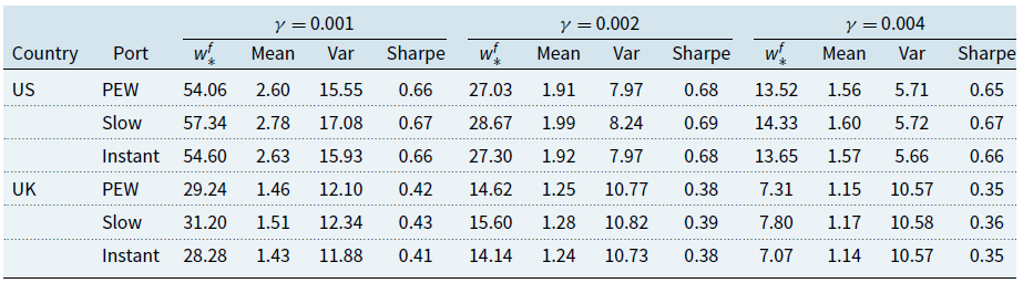
Table 2 presents the optimal mean-variance weights calculated using Eq. (15), taking into account risk aversion. Since variance-covariance parameters differ across countries, there will be a corresponding variation in the optimal funding levels. Additionally, this table includes the mean, variance, and the Sharpe ratio, which are derived from the returns of the mixed pension funds in Eqs. (19) and (20) between 2013 and 2023.
Table 2. Funding weight (%), expected return (%), variance, and Sharpe ration of the mixed pension portfolios with varying risk aversion parameters
Note: There is no statistically significant difference between the quarterly average (mean) returns of equities pre-and post-divestment (PEW vs. Slow and Instant). This finding is based on a $ t$
-test at a 99% confidence level with 39 observations for each dataset, or
$ t$
-test at a 99% confidence level with 39 observations for each dataset, or $ n_1 = n_2 = 39$
, covering a quarterly period from 2013-01-01 to 2022-07-01.
$ n_1 = n_2 = 39$
, covering a quarterly period from 2013-01-01 to 2022-07-01.
With the same risk aversion parameters, the optimal funding weight for the US is greater than that for the UK. Furthermore, slow divestment leads to the highest return and Sharpe ratio. The plot of Sharp ratio versus the log of risk aversion parameters for the US and UK can be found in Fig. 13. However, the improvement in portfolio return due to divestment does not have a statistically significant effect on the return. Specifically, the difference in mean returns pre- and post-divestment for the portfolios is not statistically significant, as evidenced by the $ t$
-test at a 99% confidence level.
$ t$
-test at a 99% confidence level.

Figure 13 Comparison of risk aversion vs. Sharpe ratio for original mixed pension portfolio vs. divested portfolio by scanning environmental risk score.
With the same risk aversion parameters, the optimal funding weight for the US is greater than that for the UK. Furthermore, slow divestment leads to the highest return and Sharpe ratio. The plot of the Sharpe ratio versus the log of risk aversion parameters for the US and UK is illustrated in Fig. 13. We find that the enhancement in portfolio return attributed to divestment does not significantly impact the return. Specifically, the difference in mean returns before and after divestment for the portfolios is not statistically significant, as confirmed by the $ t$
-test at a 99% confidence level. In addition, the maximum difference in the Sharpe ratio before and after divestment is only
$ t$
-test at a 99% confidence level. In addition, the maximum difference in the Sharpe ratio before and after divestment is only $3\%$
in the US with
$3\%$
in the US with $\gamma = 0.004$
between the PEW and the slow divestment.
$\gamma = 0.004$
between the PEW and the slow divestment.
The divestment strategy, based on environmental score scanning, at least in our case study, does not statistically affect the average quarterly return of the mixed pension fund portfolios. Even if the statistical test overlooks it, slow divestment yields both a better return and a superior return per risk for both the US and UK portfolios. Therefore, there is an incentive to prioritize divestment by scanning for environmental risks in the mixed pension fund.
6. Conclusion
This paper introduces DivFolio, an innovative and multipurpose software application for assisting investors, both retail and professionals such as portfolio and asset managers, global investment and fund managers, with ESG-related portfolio divestment decisions. The application is created in a R/Shiny environment, making it accessible to non-programmers. The software provides options for portfolio design, evaluating asset performance, creating ESG reports, comparing risk/return profiles of portfolios with and without divestment, assessing the stability of risk profiles using clustering, and examining the correlation structure via graphical lasso. The divestment capabilities distinguish DivFolio from other accessible portfolio management applications. By uploading data files, users are also able to customize the attribute for divestment, rather than only the sustainability scores that are embedded in the software, extending the tool’s application to more general divestment and portfolio comparison challenges.
A detailed set of guidelines are presented in the paper to explain the functionalities of the software and demonstrate divestment-related applications. There are two key modes offered in the software. The first mode is a sequential mode guiding users through selections of investment and divestment assets, a variety of portfolio and divestment strategies and analytics. The second mode is standalone and consists of three optional functionalities that can be executed individually. The first functionality (Option I) compares risk profiles and attributes of multiple portfolios, contrary to pairs of portfolios attained from the first mode. The second functionality (Option II) provides cluster analysis to determine the stability of portfolios risk profiles over time, offering a relative performance risk assessment of portfolios with and without divestment. The last functionality (Option III) compares the correlation structure between assets and portfolios. Regularization allows Graphical Lasso to extract sufficiently strong correlations, being advantageous for assessing the impact of divestment on the correlation of assets in portfolios.
We also demonstrate the applicability of DivFolio with illustrative examples that serve the purpose in such a paper as illustrating the types of results one may obtain from the tool, rather than a detailed financial case study. The first illustration utilizes the sequential mode to assess the impact of divestment on the environmental score and other attributes of small portfolios comprised of assets in the Energy, Utilities, and Healthcare sectors of FTSE100 (when divesting from the Energy and Utilities). Furthermore, the effects of the rate of divestment on the risk profiles and attributes of portfolios are examined.
Leveraging the DivFolio tool as part of our actuarial exploration, we examined the repercussions of divestment strategies on mixed pension funds within a mean-variance framework in the US and UK, with a focus on environmental risk scores. Our findings indicate that, while there are variations in returns attributed to divestment, they lack statistical significance. This emphasizes the inherent worth of environment-centric divestment strategies in pension fund management.
Divestment can be used to exert pressure on corporations to assume more social responsibility, including carbon emissions reductions, and upgrading the management of chemical waste. However, divestment can affect risk profiles and multiple attributes of portfolios. For instance, carbon divestment in ETFs may result in dividend yield penalties (Marupanthorn et al., Reference Marupanthorn, Nikitopoulos, Ofosu-Hene, Peters and Richards2022). Factors, such as the ratio of divestable assets and the quantity of capital relinquished can influence portfolios performance during divestment strategies. Indeed, divestment without planning may cause loss of wealth and tracking control. DivFolio offers a flexible and constructive assessment that would be valuable to asset and fund management considering divestment solutions.
Contributions
The authors contributed to this manuscript as follows:
-
1. PM: co-designed methodology, co-designed case studies, wrote code, and applications implementation, performed unit testing, co-wrote first draft of manuscript.
-
2. GWP: co-designed methodology, co-designed case studies, supervised code, and testing frameworks and co-designed interface, co-wrote first draft of manuscript.
-
3. EDO-H: co-designed methodology, co-designed case studies, supervised code, and testing frameworks and co-designed interface, co-wrote first draft of manuscript.
-
4. CSN: Co-designed case studies, commented methodology, and advised on synthetic test cases and commented first draft.
-
5. KAR: Co-designed case studies, commented methodology, and advised on synthetic test cases and commented first draft.
Data availability statement
The data and code that support the findings of this study are openly available on GitHub, hosted by Zenodo and accessible via the cataloged DOI https://zenodo.org/doi/10.5281/zenodo.10467310
Funding statement
This work received no specific grant from any funding agency, commercial, or not-for-profit sectors.
Competing interests
Author KAR is employed at company Fortlake Asset Management and University of Technology Sydney. Author PM, GWP, EDO-H, CSN declare none.
Appendix
A. DivFolio Software Components
DivFolio includes additional advanced features, such as stability assessments of portfolios via clustering and correlation structures via Graphical Lasso. These features are useful for investigating the impact of divestment on portfolio performance in multidimensional views. DivFolio can be used both to download relevant data using a convenient user interface and, to upload relevant historical price data or portfolio positions. Then comparisons can be drawn on various ESG-based automated or user-selected portfolio divestment actions. All outputs created by DivFolio, including ESG data collection, are conveniently made available to the user via a download to CSV or TXT option. Users can assess the benefits to their portfolio performance by taking certain divestment actions or even changing their investment strategy in comparison to their original portfolio strategy. This is readily achievable with DivFolio as the application allows users to upload their custom portfolio positions in easily prepared CSV files.
The front splash screen of DivFolio greets the user with a clear set of guidelines for the software’s purpose and functionality. Furthermore, it includes a user manual interface that provides basic instructions and a sequence of steps/actions they can take, either in a sequential manner or independently, see Fig. A.2, to begin the portfolio analysis. The first splash screen of the software is shown in Fig. A.1.

Figure A.1 Screenshots of the front splash screen of DivFolio.
As seen in Fig. A.1, the first channel, titled Welcome, is an introductory channel that describes the statement of purpose and main features of the software. The second channel, titled User Guide, gives an introduction, the guidelines for the use of the software, the structure of the CSV files that can be uploaded, and the outputs that the user can expect from each step. The software’s package dependency is also presented on this channel, which is useful for maintaining the use of this software in an R environment. The channel, titled Divestment Plan, is the main function of the software used for generating optimal portfolio selections and analytics for various portfolio strategies. This function accommodates divestment practice over multiple time frames and comparisons of various types of portfolio strategies, with and without divestment, applied for the user-selected equity asset universe of interest for investment and divestment. The last channel, titled Our Team, gives the bibliography and the contacts of contributors. The key components of DivFolio are detailed next.
A.1. DivFolio features comparison with existing portfolio analytic software
This section outlines how DivFolio complements and extends existing software packages for portfolio analytics and what novelty is introduced in DivFolio that is not available in these packages. We focus on available packages that are freely available, or the free components of commercial packages, as the intention of DivFolio is free access to all analytic involved in green finance and divestment practice.
The alternative software applications considered include Portfolio Visualizer, Personal Capital Finance, Yahoo Finance, Google Finance, and 3D Portfolio Optimiser, which are examples of outstanding open-source portfolio analysis software available online. Portfolio Visualizer and Personal Capital Finance both provide paid versions with access to additional features. Portfolio Visualizer is accessible without login or registration. Single- and multiperiod portfolio back-tests and portfolio analysis are provided for free. In addition, it offers robust capabilities for statistical models and quantitative analysis, including factor analysis, portfolio optimization, Monte Carlo simulation, and timing models. A fee is assessed for exporting the data. Personal Capital Finance provides a variety of financial tools, such as the Savings Planner and the Retirement Planner, for a specific purpose. The Socially Responsible Investing (SRI) tool is included in the payment plan. This software is exceptional for tracking real investment portfolios because the user may connect the tools to the broker. Yahoo Finance is among the largest databases for financial information and firm fundamentals, such as sustainability scores (ESG). It allows a user to compile a portfolio of prospective assets but cannot assign investment weights. The analysis is available for single assets but not for portfolio analytics. Google Finance also enables users to create portfolios. It is possible to construct the portfolio by allocating investment weight, and time; however, portfolio optimization is not permitted. Both Yahoo Finance and Google Finance are provided free of charge.
Although these software applications are advantageous for investors, they do not emphasize divestment and ESG investing. 3D Portfolio Optimiser, provided by ESG for Investors, is one of the tools that aims directly to perform assessments on ESG investing. It identifies the optimal portfolio allocation in terms of predicted return, risk, and climate effect based on Meinshausen & Melin (Reference Meinshausen and Melin2020), Kilmurray et al. (Reference Kilmurray, Meinshausen and Melin2021). They also offer Engagement Maximiser, a tool for investigating company sustainability scores. A limitation of the proposed tools is that the studying time cannot be customized. In other words, they provide only a single period or static portfolio optimization. Most of DivFolio’s features are centered on dynamically comparing the multiperiod portfolio’s characteristics and risk profiles, particularly in divestment and ESG investment. DivFolio also allows users to construct and compare a portfolio with a divested portfolio. The advanced comparisons include the stability analysis via clustering, as given in Section 3.2, and the strength of the correlation structure analysis, as reported in Section 3.3. The divestment functions and these advanced features distinguish DivFolio from other software programs. DivFolio does not allow users to connect to the commercial broker as it is not a real-time update application. The features comparison of the above-mentioned software applications is summarized in Table A.1.
Table A.1. Features comparison of available open portfolio analytics software

The available features were observed on 25/09/2022. Additional features may be developed after that date.
![]() means the feature is available without charge.
means the feature is available without charge.
![]() means the feature is unavailable.
means the feature is unavailable.
![]() means the feature is available with a charge for accessing.
means the feature is available with a charge for accessing.
A.2. User guideline
DivFolio can be used in two different modes of operation. The first mode is a sequence of steps that guide the user through the selection of assets for investment and divestment and sets up a variety of portfolio strategies, divestment strategies, and analytics, as shown on the left-hand side of DivFolio’s workflow displayed in Fig. A.2. This part consists of Steps 1 through 5, which must be executed sequentially. The final result of this part is a comparison of attributes and risk profiles between divested and original portfolios. The available risk profiles in DivFolio include return, cumulative return, volatility, Sharpe ratio, value at risk, max drawdown, and Sortino that enter a multiperiod portfolio optimization. If a CSV data file is prepared, users can upload it instead of producing it using the program. The uploaded files must be in the format specified in the user instructions.

Figure A.2 Workflow of DivFolio.
The second mode of operation involves advanced analytics tools, consisting of three optional parts that can be operated independently. This mode is displayed on the right-hand side of DivFolio’s workflow in Fig. A.2. This part allows users to generate a comparison of multiple portfolios, contrary to pairs of portfolios attained from the first mode of operation. More advanced comparisons, stability analysis via clustering, and graph structure of correlation are also provided. These advanced features allow the user to use DivFolio for assessing portfolio stability under different divestment decisions, assessing risk and return performance and changes in ESG and portfolio carbon footprint during divestment. Furthermore, a graph diversification-based analytics tool based on graphical lasso helps identify changes in diversification between assets in a portfolio as divestment evolves over time.
These independent functions require users to have prepared data for uploading, either from their existing portfolios or from outputs by the first mode of operation, as presented on the right-hand side of Fig. A.2. The detailed guidelines and instructions for file preparation (from the software, or via the user mapping their existing portfolio) into the required format for uploading to DivFolio are also provided to users, as detailed next.
A.3. Format of uploading CSV files
As it can be observed in the workflow diagram of Fig. A.2, the CSV files F0 to F6 can be uploaded to the tool. In practice, it is recommended to upload the files, as this will substantially accelerate the process and prevent blockage caused by excessive API data calls. In the sequential steps, the CSV files are optional, but they are compulsory in the independent functions. The format of the uploaded CSV files follows.
-
F0: List of tickers and their investment statuses This file is optional and requires: (i) a compulsory column name ‘Ticker’, consisting of tickers of all potential assets, and (ii) an optional column name ‘Status’, containing the investment status either as ‘Invest’ or ‘Divest’.
-
F1: List of tickers, their investment statuses, and some numerical attributes This file requires: (i) a compulsory column name ‘Ticker’, consisting of tickers for all potential assets and (ii) a compulsory column name ‘Status’, containing the investment status either as ‘Invest’ or ‘Divest’, and (iii) at least one column of any name that contains numerical attributes of the asset.
-
F2: Table of assets return This file requires: (i) a compulsory column name ‘Date’, consisting of dates in the form ‘year-month-day’, and (ii) other columns that are named by the ticker symbols of the selected potential assets in F1, containing the return of each asset over time.
-
F3: Table of portfolio weight This file requires: (i) a compulsory column name ‘Date’, containing dates of portfolio rebalancing in the form ‘year-month-day’ and (ii) other columns that are named by the tickers in the same order as in F2, containing the investment weights of each asset over time.
-
F4: Table of divestment schedule This file requires: (i) a compulsory column name ‘Date’, containing dates of portfolio rebalancing in the form ‘year-month-day’, and (ii) a compulsory column name ‘Bound’, containing the sequence of limits of the investment weight of the divestable assets.
-
F5: Table of portfolio weight with multiple portfolios This file requires: (i) a compulsory column name ‘Date’, containing dates of portfolio rebalancing in the form ‘year-month-day’ and (ii) a compulsory column name ‘PORTNAME’, containing any name of the portfolio as the label for separating data by portfolio type, and (iii) other columns that are named by the tickers, containing the investment weights of each asset over time.
-
F6: List of tickers and their investment statuses This file requires: (i) a compulsory column name ‘Ticker’, consisting of tickers of all potential assets, and (ii) a compulsory column name ‘Status’, containing the investment status either as ‘Invest’ or ‘Divest’.
See Figs. B.1–B.8 for examples of each of these files. It is required that the column names of each file are named exactly as provided in the quotes defined above and as demonstrated in the example files in the folder named “Example Files for Paper”.
A.4. Sequential component
Sequential steps are used for generating portfolios with and without divested assets and for comparing their performance and risk profiles. In this part, users would be able to generate portfolios and experiment with divestment strategies or upload optional CSV files for assessment. It requires progressing from Step 1 through Step 5, as discussed below.
Step 1: Asset Performance Investigation
This step is optional for users who wish to investigate the performance of assets and add them to portfolios. The list of potential assets will be added to the portfolio in Step 2.
Users should enter the ticker in the drop-down menu of the Gear icon to retrieve the selected company’s information, see Fig. B.1 for an example. The ticker must adhere to the Yahoo Finance format, i.e., the abbreviation of the market, except for U.S. markets. For example, XOM is the ticker of Exxon Mobil Corporation on the NYSE, SHEL.L is the ticker for Shell plc. on the LSE, and 600028.SS is China Petroleum & Chemical Corporation in Shanghai. Users should enter the ticker in the drop-down menu of the Cart icon to add the asset to the portfolio that would appear in Step 2. The ticker needs to be added one by one, and it is not case sensitive. The outputs of this step include foundation data of the company, such as dividend yield, currency, and market, the ESG scores, the candlestick of asset prices, and the risk profiles in different time windows.
Step 2: Selecting Divestable and Investable Assets
This step manages the assets in the portfolio and assigns their investment status. The investment status can be ‘Divest’ for divestable assets, or ‘Invest’ for investable assets. The potential assets are assigned in Step 1 unless CSV files are uploaded with user-defined assets selection. The investment status can be assigned by dragging and dropping between the panel’s prospective investable and divestable assets, as displayed in Fig. B.2. The assets in the panel, referred to as Potential Assets, are excluded from the final portfolio. To retrieve the sector, sub-sector, and ESG scores, users should click the green button, labelled summary. Once the investment status of the assets or the asset universe is updated, users should click the green button, labeled update summary. The option Manage Divestment allows a user to automatically assign the investment status to the assets in the portfolio by ranking them by the quantile of the selected attribute, such as ESG score. The ranking can be done in ascending or descending order. Another feature of DivFolio is “Selecting Assets from World Major Indices”. This functionality facilitates the retrieval of tickers associated with constituents in various global indices, eliminating the need for manual input. We recommend that users avoid frequent downloading of data, as the IP address may be blocked due to the query limitations of the API architecture. After obtaining the sustainability and sector data for the tickers, it’s possible that some company data might be unavailable. To ensure a smooth transition to Step 4 and avoid portfolios with missing sustainability weights during optimization, it’s essential to clear out these gaps. The “remove NA rows” button serves this purpose effectively.
If users have uploaded CSV files, F0 or F1 can be used in this step. If the list of tickers is available, users should upload F0. The investment status column is optional. This file allows users to add multiple tickers at once, rather than individually in Step 1. After uploading, users should click the green summary button to obtain the ESG scores. File F1 necessitates the tickers column, the status column, and at least one numeric column of attributes. This file enables users to examine the impact of divestment on other attributes besides ESG scores. If this file is uploaded, the result will be automatically calculated. The file F0 is uploaded via the Gear icon dropdown, whereas the file F1 is uploaded via the Check icon dropdown. Fig. B.2 depicts an example of uploading CSV files, where note that the highlighted columns are required.
The outputs of this step are twofold.
-
Table of Attributes shows the uploaded CSV file of investment status or the table of ESG scores, where the data is downloaded from the network. This table can be saved locally as an F1 file.
-
Comparison of Attributes Before-After Divestment in Percentage displays the score of attributes before and after divestment, as a percentage of change, under the assumption that all assets are equally weighted. The associated formula is given by
(A1)where \begin{equation} R = \frac{A_{after} - A_{before}}{A_{before}} \times 100\%, \end{equation}
$A_{before}$
and
$A_{after}$
is the attribute of the asset before and after divestment, respectively.
\begin{equation} R = \frac{A_{after} - A_{before}}{A_{before}} \times 100\%, \end{equation}
$A_{before}$
and
$A_{after}$
is the attribute of the asset before and after divestment, respectively.


Step 3: Batching Historical Data
This step retrieves the historical prices of the assets from portfolios selected in Step 2. To download historical prices, users should enter the range of dates in the Calendar icon’s drop-down menu. The historical stock prices provided are confined to trading days, excluding nonoperational market days. The date entered into the software designates the first and last available price dates, not the return dates, yielding returns for the operating day following the input date. This clarification is crucial for precise data interpretation and analysis within the software. Optionally, users can upload file F2 on Check icon’s drop-down menu. A demonstration is presented in Fig. B.3.
The outputs from this step are as follows.
-
Table of Historical Relative Return shows the return uploaded from a CSV file of historical data or the relative returns of data downloaded from the network. The relative return (RR) is calculated by
(A2)where
\begin{equation} RR = \frac{P_{t+1} - P_{t}}{P_{t}}, \end{equation}
$P_{t+1}$
and
$P_{t}$
are the adjusted closing prices at time
$t+1$
and
$t$
, respectively. This table can be saved locally as an F2 file.
-
Table of Assets Performance displays the average of asset performances over the selected period.
-
Missing Data Handling displays a heatmap of missing data, aiding users in identifying the absent information. Users are offered three alternatives for managing missing data: removing rows with absent data, substituting missing data with zero, or applying linear interpolation. It is crucial to note that the presence of missing data can lead to skewed and unreliable results.
-
Distribution of Asset Returns presents the distribution of the returns of the assets over the selected period.


Users can also select the picker option, labeled Arranging Plot, to sort the assets according to the selected performance.
Step 4: Constructing Investment Portfolios
Step 4 is used for constructing investment portfolios from assets selected in Steps 2 and 3. To generate the associated portfolio weights, users should click the Chart icon’s drop-down menu. The available options of portfolio construction methodologies include Passive Equal Weight, Active Equal Weight (AEW), Global Minimum Variance (GMV), Maximum Sharp Ratio (MS), and Principle Portfolio (PC). Further exposition of these methodologies is presented in Section 3.1. The Limit Short-Selling Weight option can be utilized to minimize leverage risk by limiting the short-selling ratio, $SL$
, in the Short-Selling Limit textbox, as illustrated in Fig. B.4. This option is based on the box constraints methodology that is presented in Eqs. (5) and (4). Rebalancing Frequency [in a day] is the number of days for the portfolio rebalancing window. This number should not exceed the number of days during the study period. Number of Days for Calculating Weights represents the number of days used in the past to calculate average return and a covariance matrix.
$SL$
, in the Short-Selling Limit textbox, as illustrated in Fig. B.4. This option is based on the box constraints methodology that is presented in Eqs. (5) and (4). Rebalancing Frequency [in a day] is the number of days for the portfolio rebalancing window. This number should not exceed the number of days during the study period. Number of Days for Calculating Weights represents the number of days used in the past to calculate average return and a covariance matrix.
If the file F3 with the portfolio weights for each rebalancing period is available, then users can upload it by clicking at the Check icon’s drop-down menu. The tool then automatically provides results. This feature allows users to apply any rebalancing portfolio mechanism by uploading a user-defined file, rather than using the portfolios generated by DivFolio.
There are ten outputs from this step, as listed and explained below.
-
Table of Rebalancing Portfolio Weight shows the portfolio weights uploaded from the CSV File of Portfolio’s Weight or portfolio weights for each rebalancing period where the portfolio weights are generated from the tool. This table can be saved locally as the file F3.
-
Time Series of Asset Weight displays the plot of the individual asset over time. Users can observe the dynamic behavior of each asset across time.
-
Assets Allocation presents the charts of portfolio weights at a given time, by using Select Date. Users can also observe the attribute of each asset by using the picker Select Factor.
-
Attribute Allocation in Portfolio displays the plot of the attribute weighted by portfolio weights,
(A3)where
\begin{equation} EA = \sum _{i = 1}^N w_iA_i, \end{equation}
$N$
is the portfolio’s asset count,
$w_i$
is the asset’s investment weight, and
$A_i$
is the asset’s attribute. It can be seen as the expected attribute, namely EA, and can be calculated for short and long positions separately. In this chart, users observe the behavior of the portfolio’s expected attribute over time.
-
Distribution of Attributes for Long Position and Distribution of Attributes for Short Position show the boxplots of distribution of attributes separated by holding positions. The white dot represents the average value of the distribution. item[Table of Time Series of Attributes] displays the expected attribute of the portfolio over time separated by holding positions.
-
Distribution of Portfolio Risk Profiles shows the boxplots of distribution of portfolio’s performances over the sample period. The white dot represents the average value of the distribution.
-
Efficiency Frontier displays the plot of portfolio standard deviation versus return. The picker has multiple options that allow the user to observe many curves in the same plot.
-
Table of Risk Profiles summarizes the table of risk profiles calculated backward before each rebalancing over time.
-
Time Series of Risk Profiles displays the plot of risk profiles calculated backward before each rebalancing over time.


Step 5: Divestment
The divestment step involves allocating funds proportionally from the divestable assets to the investable assets, as detailed in Marupanthorn et al. (Reference Marupanthorn, Nikitopoulos, Ofosu-Hene, Peters and Richards2022). This section constructs divested portfolios based on portfolios generated in Step 4, and the divestment schedule – the maximum investment weights for divestable assets at a given time. To construct the divestment schedule and divested portfolio, users should navigate to the Minus icon’s dropdown menu; see Fig. B.5. The three possible rates of divestment are given as options: Instant, Linear, and Hyperbolic, see Eqs. (6), (7), and (8), respectively. Accordingly, users should select one of the options, then set parameters, and finally, click the submit button to generate a divestment schedule and divested portfolios.
If the F4 file of the divestment schedule is accessible, then it can be uploaded through the Check icon’s drop-down option in order to acquire the divested portfolio. This option allows users to specify the divestment schedule – that would differ from the rates of divestment offered in DivFolio.
Most of the outcomes of this step resemble those of Step 4. In addition, the comparison of the original portfolio with the divested portfolio is included in Step 4. The additional outputs from Step 5 are listed below.
-
Table of Divestment Schedule shows the divestment schedule uploaded from CSV File of Divestment Schedule or the divestment schedule generated by DivFolio. This table can be saved as an F4 file.
-
Portfolio Weight After Divestment shows the weights of the divested portfolio over time according to the divestment schedule.
-
Sum of Weights of Divestable shows the chart of the sum of the weights of divestable assets over time. It is observable that the divestable assets decrease over time, as the capital is allocated to the investable assets. The weights allocated to the investable assets are equivalent to the difference between the weights in the divestable assets and the divestment boundary in line with the divestment schedule (10).
-
Sum of Allocated Weights and Investable Assets Weights presents the chart of the sum of the weights allocated from the divestable and investable asset weights. This is the sum of the new weights of the investable assets in the divested portfolio at a certain time (see Eq. (11)).
-
Distribution of Percentage of Relative Change between non-divested and divested portfolios displays the boxplots of the distribution of the percentage of non-divested and divested portfolios spread out. It is calculated by
(A4)where
\begin{equation} PR = \frac{AP_{divest} - AP_{non-divest}}{AP_{non-divest}} \times 100\%, \end{equation}
$AP_{non-divest}$
and
$AP_{divest}$
are the attribute or risk profile of the portfolio, before and after divestment, respectively.


B.5. Independent component
The functions of the independent component operate separately from the others, thus users have access to Option I, Option II, and Option III without having to preoccupy other panels. For the functionalities to execute, the data download must be completed before operating and a certain CSV file format is required.
Option I: Multiple Portfolios Comparison
The objective of this panel is to compare the results of risk profiles and attributes of multiple portfolios. The necessary files that should be uploaded include the file of portfolios weight (F5), the file of historical return (F2), and the file of asset attributes and investment status (F1), as shown in Fig. B.6. The majority of functions are similar to Step 5, but this step allows for comparisons of multiple portfolios. The multiple comparison functions added in this panel are Table of Percentage of Relative Change compared to Benchmarks and Distribution of Percentage of Relative Change compared to Benchmarks which are the table and plot of the percentage of relative change compared to benchmarks. It captures the difference between the benchmark portfolios and others. The associated formula is given by
 \begin{equation} PR = \frac{AP_{other} -AP_{benchmark}}{AP_{benchmark}} \times 100\%, \end{equation}
where $AP_{benchmark}$
and
$AP_{benchmark}$
and $AP_{other}$
are the attribute, or risk profile of the benchmark, and comparing portfolio, respectively. More than one benchmark portfolio can be selected. The non-benchmark portfolios are compared to the nearest benchmark portfolio located before them. The names of portfolios are arranged according to the input CSV file.
$AP_{other}$
are the attribute, or risk profile of the benchmark, and comparing portfolio, respectively. More than one benchmark portfolio can be selected. The non-benchmark portfolios are compared to the nearest benchmark portfolio located before them. The names of portfolios are arranged according to the input CSV file.
Option II: Stability Analysis via Clustering
This optional panel is used to assess the stability performance of portfolios. To investigate stability, we apply CLARA, a close approximation to k-medoids methods (discussed in Section 3.2). Clustering was performed using the following criteria: return, cumulative return, volatility, Sharpe ratio, value at risk, maximum drawdown, and Sortino. CLARA is used to cluster the aggregation time series of risk profiles using a $\tau$
-day time window. Every
$\tau$
-day time window. Every $t$
day, the clustering algorithm is applied. These parameters are configurable within DivFolio. The clustering silhouette identifies the ideal number of clusters. Over time, portfolios with similar relative performance would belong to the same cluster.
$t$
day, the clustering algorithm is applied. These parameters are configurable within DivFolio. The clustering silhouette identifies the ideal number of clusters. Over time, portfolios with similar relative performance would belong to the same cluster.
To access this function, the required CSV files, F5 and F2, need to be uploaded on the Check icon’s drop-down menu. Users should enter the number of days in the time window, $\tau$
, and the number of days in cluster analysis,
$\tau$
, and the number of days in cluster analysis, $t$
, to process the function. Fig. B.7 displays an illustration of Option II.
$t$
, to process the function. Fig. B.7 displays an illustration of Option II.
The outcomes of this optional panel are as follows:
-
Table of Aggregate Time Series of Risk Profiles displays the aggregate time series of risk profiles of portfolios over time.
-
Time Series of Risk Profiles shows the plots of the aggregate time series of risk profiles of portfolios over time.
-
Table of Clustering Silhouette depicts the silhouette information of clustering. The column name is the number of clusters.
-
Clustering Results display the heatmaps of the clustering of all portfolios over time. The number inside the cells and color represent the label of the cluster.
Option III: DivFolio Portfolio Diversification via Graphical Structure Correlation Analysis
The Option III panel can be used to investigate the correlation structure of the assets in portfolios using the graphical least absolute shrinkage and selection operator (glasso) Zhao et al. (Reference Zhao, Liu, Roeder, Lafferty and Wasserman2012), as detailed in Section 3.3. To assess the correlation structure in DivFolio, the covariance matrix of $N$
asset returns weighted by their investment weight should be generated as follows:
$N$
asset returns weighted by their investment weight should be generated as follows:
 \begin{equation} \tilde{\Sigma }_{ij} = \text{cov}(w_ir_i,w_jr_j) = w_iw_j\text{cov}(r_i,r_j), \end{equation}
where $w_i$
and
$w_i$
and $w_j$
are the investment weights and
$w_j$
are the investment weights and $r_i$
and
$r_i$
and $r_j$
are the returns of the asset
$r_j$
are the returns of the asset $i$
and
$i$
and $j$
, for
$j$
, for $i,j = 1,\dots,N$
. The optimization in (12) is resolved by setting
$i,j = 1,\dots,N$
. The optimization in (12) is resolved by setting $S = \tilde{\Sigma }$
, resulting in the optimally estimated sparse covariance matrix. The optimal
$S = \tilde{\Sigma }$
, resulting in the optimally estimated sparse covariance matrix. The optimal $\lambda$
is calculated by the package “huge”, see Zhao et al. (Reference Zhao, Liu, Roeder, Lafferty and Wasserman2012). Under the provided regularization parameter, the links in the network of the produced sparse matrix suggest a correlation between the assets in the portfolio that is sufficiently strong.
$\lambda$
is calculated by the package “huge”, see Zhao et al. (Reference Zhao, Liu, Roeder, Lafferty and Wasserman2012). Under the provided regularization parameter, the links in the network of the produced sparse matrix suggest a correlation between the assets in the portfolio that is sufficiently strong.
To access this function, the CSV files F5 and F2 are required. The file F6 is optional. Users should navigate to the Check icon’s drop-down menu to upload those files, see Fig. B.8.

Figure B.1 Input management in Step 1.
The associated output includes Covariance Portfolio Network Structure that illustrates the graph network generated from the estimated sparse covariance matrix calculated using the glasso algorithm. The tool enables the user to compare structures over three-time steps. Users should select a time in the picker, select Date, and click the submit button to execute the algorithm. The asset’s correlation is shown by the link, whose thickness indicates its strength. Red and green, respectively, represent the negative and positive associations. The network’s nodes represent assets, and their colors indicate investment status if file F6 was submitted. The investable assets are depicted in blue, while the divestable assets are depicted in yellow. The labels of nodes are arranged alphabetically and anticlockwise, with the first node positioned in the top-center position. It should be emphasized that the method can be computationally expensive even for a relatively small portfolio. Thus, the computation time is dependent on the number of assets and portfolios.
B. Input Windows and Uploading Files Format

Figure B.2 Input management in Step 2.

Figure B.3 Input management in Step 3.

Figure B.4 Input management in Step 4.

Figure B.5 Input management in Step 5.

Figure B.6 Input management in Option I.

Figure B.7 Input management in Option II.

Figure B.8 Input management in Option III.
C. List of R Packages Integrated in DivFolio
Table C.1. List of the packages used for developing DivFolio


 Open access