


INTRODUCTION
Cryo-seismology has become a popular approach to study glacier dynamics (see reviews of Podolskiy and Walter, Reference Podolskiy and Walter2016; Aster and Winberry, Reference Aster and Winberry2017, and references therein). Seismic records allow observing glacial processes and inferring englacial and subglacial conditions in previously inaccessible areas, independent from visibility conditions, over a wider area than point measurements at boreholes, and with high temporal resolution. While strong cryogenic seismic signals, such as those generated by iceberg calving at glaciers and icestreams, are observed at ranges up to regional and even teleseismic distances (e.g. Ekström and others, Reference Ekström, Nettles and Abers2003; O'Neel and others, Reference O'Neel, Larsen, Rupert and Hansen2010; Köhler and others, Reference Köhler, Nuth, Schweitzer, Weidle and Gibbons2015), local glacier microseismicity, mainly related to brittle ice failure (crevasse opening) and basal processes (e.g., stick-slip), is best monitored with stations installed on the ice surface or in shallow boreholes (e.g. West and others, Reference West, Larsen, Truffer, O'Neel and LeBlanc2010; Walter and others, Reference Walter, Canassy, Husen and Clinton2013; Röösli and others, Reference Röösli2014; Helmstetter and others, Reference Helmstetter, Nicolas, Comon and Gay2015b). In this study, we analyze a 4.5-months-long record of a single three-component seismic sensor deployed on a glacier on the Arctic archipelago of Svalbard (74–81°N, 10–35°E) in 2016. We detect and group icequakes, and use waveform polarization analysis and seismic waveform modeling to investigate the nature of their sources. The aim of this study is to show how the analysis of glacier seismicity from a single station (Helmstetter and others, Reference Helmstetter, Moreau, Nicolas, Comon and Gay2015a; Gajek and others, Reference Gajek, Trojanowski and Malinowski2017) can generate insight into related glacier surface and dynamic processes, as a cost-effective preparation for larger deployments or in remote areas where a network deployment is not feasible for logistical reasons.
DATA AND STUDY AREA
We use a passive seismic record collected between 14 April and 27 August 2016 with a temporary seismic station (HDF in the following) deployed on Holtedahlfonna, a 368 km2 (Nuth and others, Reference Nuth2013) ice field in Northwest Svalbard (Fig. 1), that drains through Kronebreen into Kongsfjord about 15 km East of the research settlement of Ny Ålesund. Kronebreen is one of the fastest marine-terminating glaciers in Svalbard with annual frontal ablation between 0.2 and 0.5 km3a−1 within the past 15 years (Schellenberger and others, Reference Schellenberger, Dunse, Kääb, Kohler and Reijmer2015; Köhler and others, Reference Köhler2016) which is 96% of the total annual ice loss of the glacier (Nuth and others, Reference Nuth, Schuler, Kohler, Altena and Hagen2012). The seismic installation was located 15 km upstream from the terminus of Kronebreen at 13.2126°E, 78.9064°N and at 520 m elevation. The recording unit was a 4.5 Hz three-component geophone (SENSOR PE-6/B) connected to a Omnirecs DATA-CUBE data logger operating with a sampling frequency of 100 Hz and using a 12 V, 57 Ah AGM battery as power supply. Station HDF was located in the ablation zone where the ice surface is exposed during summer, at about 10 km distance downstream from the summer snow line (Winsvold and others, Reference Winsvold2018). The snow layer was ~2 m thick during installation in April. After digging a snow pit, a borehole was drilled 1 m into the ice to accommodate the geophone. The borehole was filled with water to freeze the instrument in and couple with the glacier ice. After refilling the snow pit, the battery and data logger were placed on top of the snow surface, co-located with a dual-phase global navigation satellite system (GNSS) receiver. The seismic instrument recorded until battery drainage at the end of August, and the data logger was retrieved a few weeks later, the geophone still being frozen in the ice. The temporary deployment was a pilot study to access the potential of on-ice installations on glaciers in Svalbard using a simple and low-cost instrumental setup. For logistical reasons, no further geophones were installed on the glacier that year. Glacier velocity data from the GNSS receiver is only available between 29 June and 17 July 2016 due to instrumental failure.
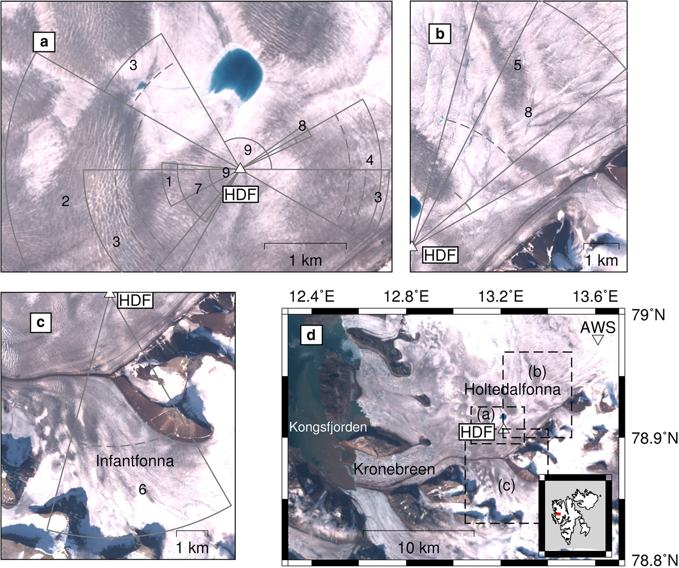
Fig. 1. Study area. (a)–(c) Location of seismic station HDF and source areas of glacier seismicity. Sectors indicate directions for each group of observed icequakes. Group numbers can appear several times in different panels since different master events are merged into a single group. Dashed arc segment is estimate of lower and solid arc of upper epicentral distance for each group. (d) Location of study area in Svalbard (lower right corner) and extent of maps in (a)–(c). Inverted triangle is location of automated weather station (AWS). Background images: Copernicus Sentinel 4 August 2016 20:03:58.
Air temperature and solar radiation measurements are available from an automatic weather station at 12 km distance, upstream of HDF (13.6115°E, 78.9805°N). Furthermore, we compare the observed seismicity with modeled meteorological and glacier mass-balance variables using a method similar to Van Pelt and Kohler (Reference Van Pelt and Kohler2015). As in Van Pelt and Kohler (Reference Van Pelt and Kohler2015), a coupled energy balance -- multi-layer snow model is used, driven by downscaled meteorological fields from the High Resolution Limited Area Model (HIRLAM Reistad and others, Reference Reistad, Breivik, Haakenstad, Aarnes and Furevik2009; Van Pelt and others, Reference Van Pelt2016). Here, we use 3-hourly and daily output of rainfall, snowfall, air temperature, snow mass, runoff and melt on a 1 km x 1 km grid. The subsurface routine accounts for density, temperature and water content changes after water percolation, refreezing and storage. Runoff is modeled as the local amount of water available at the base of the snow/firn pack and entering the glacier after potential refreezing or storage in the snow pack, if present. No transport of water from upstream is included.
STA/LTA EVENT DETECTION AND SEISMIC NOISE
In order to detect and categorize glacial seismicity in the HDF record, we utilized a short-term over long-term average (STA/LTA) trigger (Withers and others, Reference Withers1998) and master event cross-correlation (described in the next section), two methods which are common in glacial seismology (e.g. Stuart and others, Reference Stuart, Murray, Brisbourne, Styles and Toon2005; Carmichael and others, Reference Carmichael, Pettit, Hoffman, Fountain and Hallet2012; Röösli and others, Reference Röösli, Helmstetter, Walter and Kissling2016a). First, we applied the STA/LTA detector on bandpass-filtered data (1–50 Hz) to obtain an overview of the recorded seismicity using a STA length of 0.5 second, LTA length of 15 second, and STA/LTA threshold of 4.0 (Fig. 2). The detector parameters were found by testing different settings, requiring that most seismic events in representative, visually screened parts of the record are detected. We also computed seismic background noise levels by averaging seismogram envelopes of all three components (Z,N,E) over 1 hour after excluding time samples where the STA/LTA threshold was exceeded.
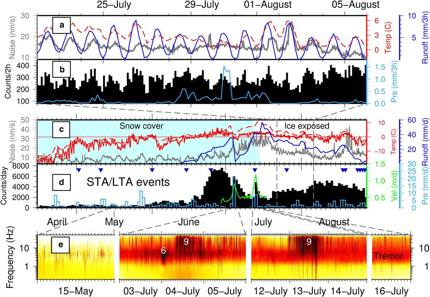
Fig. 2. Glacier seismicity at HDF. (a) Seismic background noise excluding detected events for 2 weeks (gray curve). (b) STA/LTA trigger event counts per 2 hours for 2 weeks. Precipitation, temperature, and runoff in (a) and (b) are modeled at HDF. (c) Seismic background noise at HDF (gray curve). Average air temperature is measured 12 km upstream of HDF (solid line) and modeled at HDF (dashed). Runoff is modeled at HDF. (d) STA/LTA trigger event counts per day. Daily precipitation modeled at HDF and glacier flow velocity at HDF from GNSS measurement are shown. Inverted triangles: Days visually inspected for seismic signals. (e) Spectrograms of different days distributed over the recording period. Red indicates high seismic amplitudes. Numbers refer to event groups predominantly visible as high-amplitude features at different frequencies. Amplitude decay at low frequencies is due to decreasing instrument sensitivity below 4.5 Hz.
Figure 2 provides a summary of the detections together with meteorological and glaciological observations and model output variables at HDF, and zooms on particularly interesting time periods. Figure 2d shows the temporal distribution of all seismic STA/LTA detections at HDF (black histograms). We detect about 400 events per day from April to the end of May, followed by an increase shortly after strong rain events. During the second half of June, the detection rate increases strongly to ~7000 events per day simultaneously with air temperatures staying above 0 °C. In July and August seismicity decreases to rates between 2000 and 5000 detections per day. Some short-term peaks correlate with fast glacier flow episodes (green curve) and strong rain events on 4 July and 13 July (blue bars). During the second half of July until August, detections exhibit a diurnal temporal distribution (Fig. 2b), correlating with variation in temperature and runoff. Figure 2e shows spectrograms of continuous seismic data in selected time periods. Icequakes are mainly visible as vertical stripes in the frequency band between 2 and 50 Hz. During glacier fast-flow periods in July, more high-frequency signals above 10 Hz are observed.
When interpreting the temporal distribution of seismic event detections, we must be aware that a changing seismic background noise level due to variability in meteorological conditions (i.e., wind and rain) and water flow affects the detection rate (Carmichael and others, Reference Carmichael, Pettit, Hoffman, Fountain and Hallet2012), and that therefore variability in event counts does not always correspond to a change in seismic activity at the source. For example, the high noise level in July (Fig. 2c) coincides with decreasing number of detections (Fig. 2d). However, noise variability is clearly not responsible for other temporal patterns that we observe such as the increase of seismicity in June and the diurnality.
In addition to increasing icequake activity, the spectrograms show a clear change in the seismic background noise character from spring to summer months (Fig. 2e). Spectral amplitudes are higher in the frequency range between 1 and 10 Hz during the melt season. The gray curve in Fig. 2c shows that noise amplitude varies over time and is highest in July when air temperatures stay above 0 °C for about 2 weeks. Noise amplitudes decrease again in the middle of July when temperatures vary ~0°. However, there are at least three episodes of positive temperatures in August when the noise amplitude also increases slightly for one or several days, most pronounced during the second half of August. The modeled runoff at HDF (blue curve in Fig. 2c) roughly follows the noise variability, although noise peaks seem to be delayed by a few days. Moreover, except during four rainy days between 28 and 31 July, noise amplitudes vary diurnally in the end of July when snow cover disappeared (light blue background color), slightly delayed with respect to runoff and number of seismic events (see zoom in Figs 2a and b). While higher noise level can be partly due to weak seismicity which is not STA/LTA-detected and therefore not excluded when averaging seismogram amplitudes, noise diurnality also shows that seismic event diurnality is not a result of the trigger sensitivity, i.e., decreased detectability due to higher noise level at night can be ruled out. On the other hand, the lower seismic detection rate in July can be a result of the high background noise level (compare Figs 2c and d).
The number of seismic signals generated by calving events at the terminus of Kronebreen lays typically between 100 and 350 events per day during highest calving activity in August (Köhler and others, Reference Köhler2016). Even though our STA/LTA trigger was not tuned to detect those signals, which have typical lengths of 10--20 second at 15 km distance (Köhler and others, Reference Köhler, Nuth, Schweitzer, Weidle and Gibbons2015), the slight increase of detections per day in August might in parts be related to calving seismicity.
CATEGORIZATION OF ICEQUAKES
The STA/LTA detections are further analyzed to identify different icequake sources. We will first describe the master event cross-correlation detection methodology and the determination of source directions. Then, a 1-D seismic velocity model at the study site is derived, required for modeling synthetic seismograms. Finally, we describe the different groups of icequakes observed at HDF and compare the signals with the synthetic waveforms.
Cross-correlation detection
In order to obtain an overview of existing event types, we first visually inspected the continuous seismic data and manually picked signal onsets for selected days spread over the entire recording period (see symbols in Fig. 2d for days). In total, we manually picked 1508 signals from which we sorted 1348 events into preliminary groups based on similar waveform characteristics such as signal length, frequency content and character of P and secondary wave onsets. In the next step, the waveform cross-correlation matrix of all picked events in each group was computed to assess signal similarity in a more quantitative and objective manner. Between 2 and 10 master events were selected from clusters of correlated signals within each group using a cross-correlation coefficient of 0.7 as a lower limit required for similarity. Events that do not correlate with more than two other events were not considered for automatic detection. Our method shares some similarities with the approach presented by Carmichael and others (Reference Carmichael, Pettit, Hoffman, Fountain and Hallet2012). However, our method is not fully automatic when it comes to the definition of signal clusters.
Next, a cross-correlation detector was applied to the entire, continuous record using all selected master events and a minimum correlation threshold between 0.55 and 0.7, depending on the icequake group (see Table 1). The cross-correlation coefficient was obtained by averaging the correlations of all three wavefield components (Z,N,E). A few preliminary event groups were merged since they exhibited similar temporal distribution and the corresponding signals arrived from similar directions (see next section), but different distances, finally resulting in nine different groups (see Table 1). Due to the vast amount of seismic signals in the record, i.e., ~325000 STA/LTA detections, our analysis is not a complete assessment of local glacier seismicity. It is restricted to repeating signals of similar waveforms, and we cannot expect to detect sporadic and/or scattered seismicity with the cross-correlation detector, although source mechanisms might be similar. Hence, the total number of cross-correlation detections is ~50% of the total number of STA/LTA detected signals. However, since the event groups are obtained from days spread over the entire measurement period and include similar signals, we expect to reveal the most active source areas and most frequent dynamic source processes at Holtedahlfonna.
Table 1. Icequake groups at HDF. NoMa: Number of master events. CT: cross-correlation coefficient threshold. Rg: short-period Rayleigh wave.

During visual inspection we found a few seismic signals that share similarities in their appearance, but exhibit dissimilar waveforms, unsuitable for master event cross-correlation detection. We refer to these icequakes as group 10 and discuss their characteristics below. However, no screening of the continuous record was feasible in this case.
Icequake source directions
Polarization analysis allows locating icequakes in single-station records (Helmstetter and others, Reference Helmstetter, Moreau, Nicolas, Comon and Gay2015a). Most event groups include signals that we can identify as P waves, S waves, or Rayleigh waves. We can exploit the fact that P waves and Rayleigh waves are polarized in the vertical plane containing the source and the seismometer to determine the azimuth of this plane with respect to North, and therefore the direction of the source location from the station, also called the back-azimuth. This can be done using the horizontal components and finding the azimuthal direction in which energy is maximized. Alternatively, we can find the azimuth in which the horizontal signal has the highest correlation with the vertical one. For Rayleigh waves, we need to account for a π/2 phase shift between the two components and perform therefore the correlation between the vertical component and the Hilbert transform of the radial one. Knowing back-azimuth, the seismograms can be expressed in the coordinate system vertical-radial-transverse. This ensures a separation of the P and Rayleigh waves, present on the vertical and radial components, from the Love waves, present on the transverse components.
We implemented an automatic procedure to measure back-azimuth from all cross-correlation detections. Since we know the time windows of P wave and secondary arrivals in the corresponding master event waveform, we can define the corresponding time windows for all detections. The directions maximizing the amplitude on the radial component of the P arrival and maximizing the cross-correlation between the vertical component and Hilbert-transformed radial component of the secondary arrivals (assuming dominant Rayleigh wave for near-surface signals) were determined. In the P wave case, the 180° back-azimuth ambiguity was avoided by searching the maximum radial amplitude within a range ±90° around the direction which maximizes the correlation between vertical and radial component in the P wave time window since those components should have the same polarity. A threshold for the maximum correlation of 0.65 was used to reject estimates of weak or mixed seismic phases, resulting in 71000 back-azimuth estimates for groups 1–8 combined in case of using secondary arrivals. In Fig. 1 we indicate schematically the azimuthal sector of source directions for each group.
Seismic velocity model
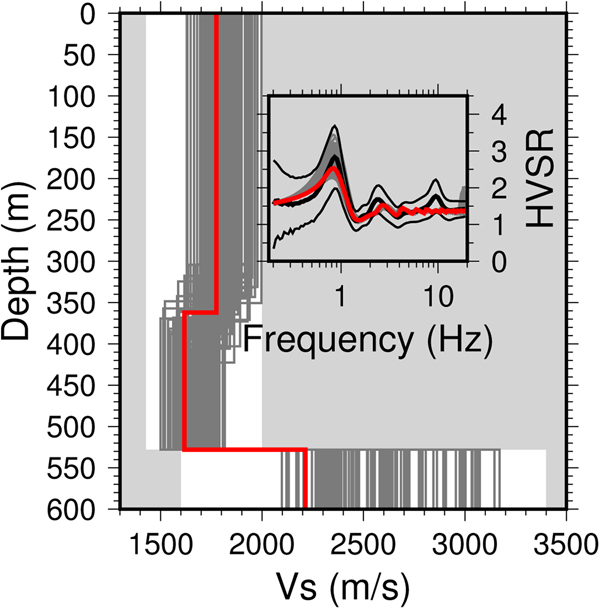
Glacier thickness at the HDF location is known from GPR measurements to be 528 m (Lindbäck and others, Reference Lindbäck2018). We used the Horizontal-to-Vertical Spectral Ratio method (HVSR, Nakamura, Reference Nakamura1989; Lachet and Bard, Reference Lachet and Bard1994; Lunedei and Malischewsky, Reference Lunedei, Malischewsky and Ansal2015; Sánchez-Sesma, Reference Sánchez-Sesma2017, and references therein) to infer the seismic velocities in the ice and below the glacier base following the approach of Picotti and others (Reference Picotti, Francese, Giorgi, Pettenati and Carcione2017) and Yan and others (Reference Yan2018). The HVSR technique is a passive seismic, single-station method that utilizes the characteristic of the continuous ambient seismic noise wavefield. We used the code of García-Jerez and others (Reference García-Jerez, Piña-Flores, Sánchez-Sesma, Luzón and Perton2016) based on the diffuse wavefield theory that allows inversion of the spectral ratios accounting for Rayleigh, Love and body waves in the noise record. After testing different parametrization (single layer and multiple layers), we finally chose a two layer over halfspace model with fixed lower depth of the second layer representing the known glacier thickness. The seismic P and S velocities, the Poisson ratios and the halfspace density were allowed to vary within realistic ranges (see Fig. 3). Ice density was fixed to 0.92 gcm−3. We inverted an averaged HVSR curve from data recorded on 17 April, since early in the season directional icequakes sources are less frequent and the diffuse wavefield assumption is more likely to be valid. Figure 3 and Table 2 present the inferred S-wave models and the HVSR fit. The best-fitting models exhibit lower seismic velocities in the second layer which indicates temperate below cold ice, which is common for Svalbard glaciers (Björnsson and others, Reference Björnsson1996). The HVSR fit above 5 Hz is poor, suggesting limited resolution at shallow depths (<50 m) which could be related to unfavorable noise characteristics at high frequencies such as lacking energy or directional sources.

Fig. 3. Measured H/V spectral ratio at HDF (black curve in inset with uncertainty) and best fitting sub-surface S wave velocity model (red). Gray models show set of best fitting models. White area indicates allowed range of Vs in inversion. The range of the other model parameters are; Vp ice: 2900–4000 ms−1; Vp halfspace: 3500–6000 ms−1; Poisson ratio ice: 0.3–0.34; Poisson ratio halfspace: 0.25–0.4; density halfspace: 1.9–2.6 gcm−3 .
Table 2. Velocity model inverted from H/V spectral ratios (Fig. 3). HS: halfspace

Synthetic seismograms
In order to further exploit the characteristic of the observed waveforms, synthetic seismograms were computed for sources of different types and different depths. For this purpose we use the reflectivity program QSEIS (Wang, Reference Wang1999) that produces complete three-component seismograms for sources and receivers located in a layered laterally homogeneous structure. We choose to use the structure obtained by the HVSR analysis in the previous section as representative for the average 1-D structure of the area around the sensor. This assumption is most likely valid for seismic waves in the vicinity of HDF and for signals traveling parallel to the glacier flow, assuming thickness is only changing slightly. For more distant sources and icequakes originated at tributary glaciers, 2-D and 3-D effects might become more important.
As several observed waveforms show dispersion, i.e., frequency depending propagation velocity, in the surface wave coda due to waveguide effects (see e.g., event group 4 below), we also tested models with low velocities at the surface, reproducing for example a zone of more crevassed ice at the surface (Lindner and others, Reference Lindner, Laske, Walter and Doran2018). The best fit is obtained using a linear gradient from the surface of the glacier to the top of the normal ice, 10 or 50 m further down. P and S-wave velocities were set at 2.0 and 1.0 km−1, respectively, at the surface, and the density at 0.8 gcm−3. We tested also models with a uniform 10 m thick low-velocity layer at the surface, with 2 m of snow cover at the surface, or with an additional low-velocity layer at the base of the ice, simulating soft bed conditions, but these models did not yield improved fit to the data and their synthetic waveforms are not shown here.
The receiver is located at 1 m depth in the ice and sources are located either close to the surface or close to the base of the glacier. We found that intermediate depth sources did not help to better constrain the source depth, and we, therefore, restrict our analysis on distinguishing between shallow and deep icequakes. The source time function is either an impulsive source (half-duration of 0.02 second) or a harmonic signal of the form sin(2π/T · t) · exp( −a · t) with different periods T. The decay constant a was chosen such that the source signal amplitude decayed to 0.1% for a specified duration of the source time function.
Waveforms shown here are generated with four basic source types (Fig. 4): opening of a vertical crevasse in horizontal direction (called Type 1 in the following), horizontal slip on a vertical plane (Type 2), opening of a horizontal cavity in the vertical direction (Type 3), and horizontal movement on a horizontal plane (Type 4). The orientation of the source fault plane with respect to the radial direction influences mostly the ratio between the transverse displacement and the vertical-radial ones. We, therefore, show only synthetics for one chosen source orientation, but discuss what the synthetics would look like for other orientations. To find source mechanisms for icequakes in our record, we perform a qualitative comparison of modeled and observed waveforms. For a good visual fit we require that the polarity of P and S phases, the dominant frequency, the presence of a coda, the S-P travel time difference, and the amplitude ratios between vertical and horizontal components are reproduced.

Fig. 4. Example of observed and modeled signals for group 3 using three different source models with shallow depths (Type 1: Opening of vertical crevasse, Type 2: Horizontal slip on vertical plane, Type 3: Opening in vertical direction, Type 4: Horizontal movement on horizontal plane), a deep source (520 m), and a shallow source in a model without a shallow seismic low-velocity structure.
Icequake groups 1–5
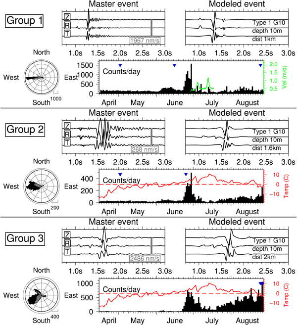
Figures 5–7 show the temporal distribution of event detections for each group together with waveforms of one or two master events and azimuthal distribution. Group 1 (Fig. 5) comprises short, high-frequency (>10 Hz) signals with duration <1 second and impulsive, clear P wave and dominant secondary wave onsets. Back-azimuth measurements and comparison with synthetic waveforms suggest a shallow source down-glacier, 800–1000 m to the West of HDF. The temporal distribution shows constant seismicity of 100--200 events per day from April until beginning of June, followed by a gradual increase until the middle of June, a slow decrease afterwards, and a sudden increase to a rate of 1000–1500 detections per day in the end of June. In July and August seismicity decreases to a level comparable to spring, however, interrupted by day-long peaks, two of them during fast glacier flow episodes (4 and 13 July). Groups 2 and 3 (Fig. 5) show similar temporal distribution as group 1, however, waveforms suggest a more distant source downstream of HDF, in the area of a large crevasse field (Fig. 1). Difference between group 2 and 3 is a stronger coda for group 2, source areas in different parts of the crevasse field, and group 3 showing much stronger and gradually increasing activity from the end of July until August. Combined, groups 2 and 3 have a similar number of events per day as group 1.

Fig. 5. Icequakes observed at HDF in groups 1-3. Panels show one master event, the modeled signal, back-azimuth distribution, and temporal distribution. Colored lines: Modeled air temperature in event source area and glacier flow velocity from GNSS measurements at HDF. Inverted triangles indicate timing of all master events in group. Rose diagram shows source directions estimated from secondary arrivals assuming Rayleigh waves (black) and obtained from P arrivals (gray). Gray bar in master event panel indicates amplitude scale in ground velocity. Source type, depth and epicentral distance are given in panel of modeled event. ‘G10’ stands for sub-surface model with a seismic velocity gradient in the upper 10 m.
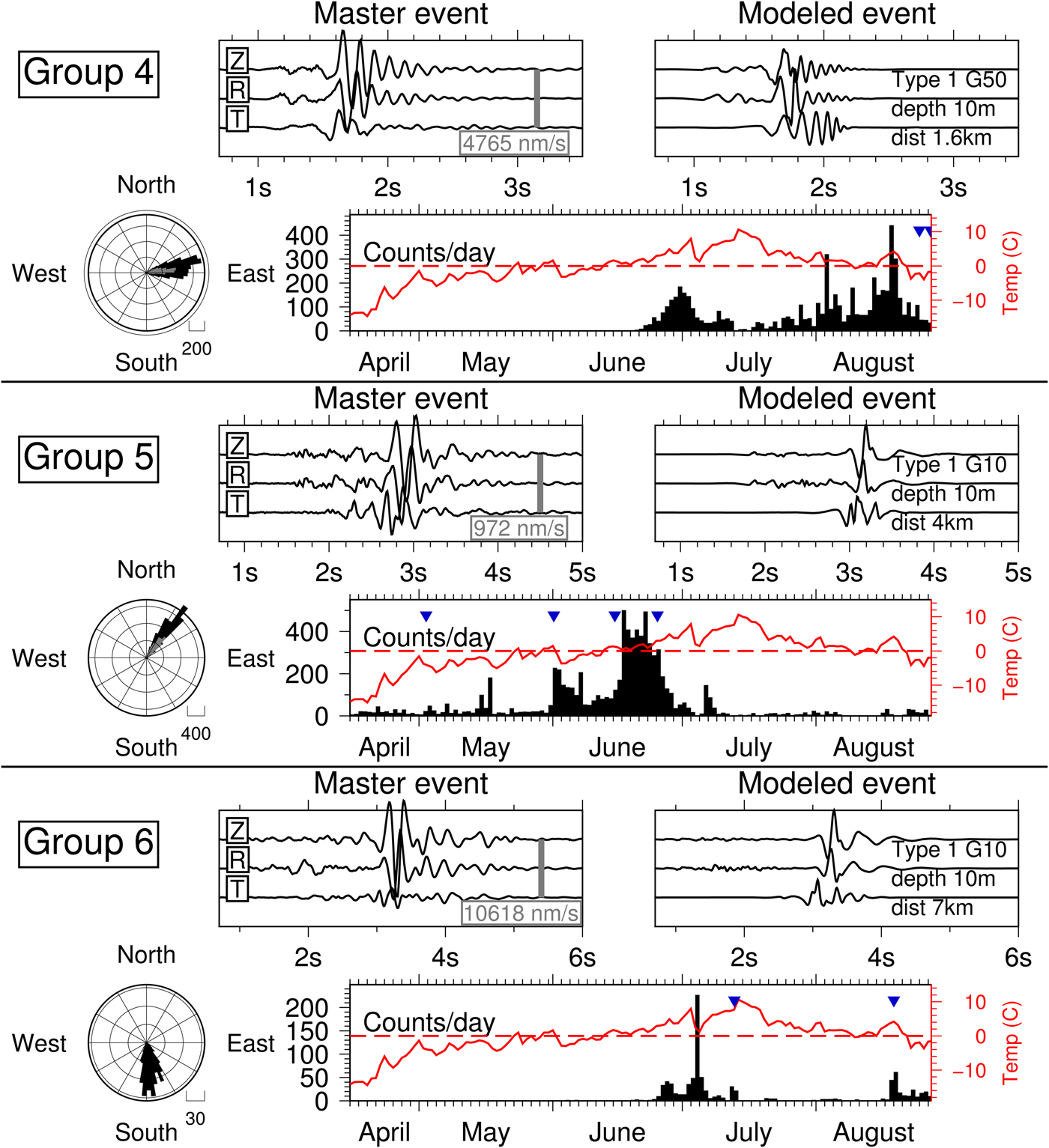
Fig. 6. Icequakes observed at HDF in groups 4–6. See explanation in caption of Fig. 5. ‘G50’ stands for a seismic velocity gradient in the upper 50 m.
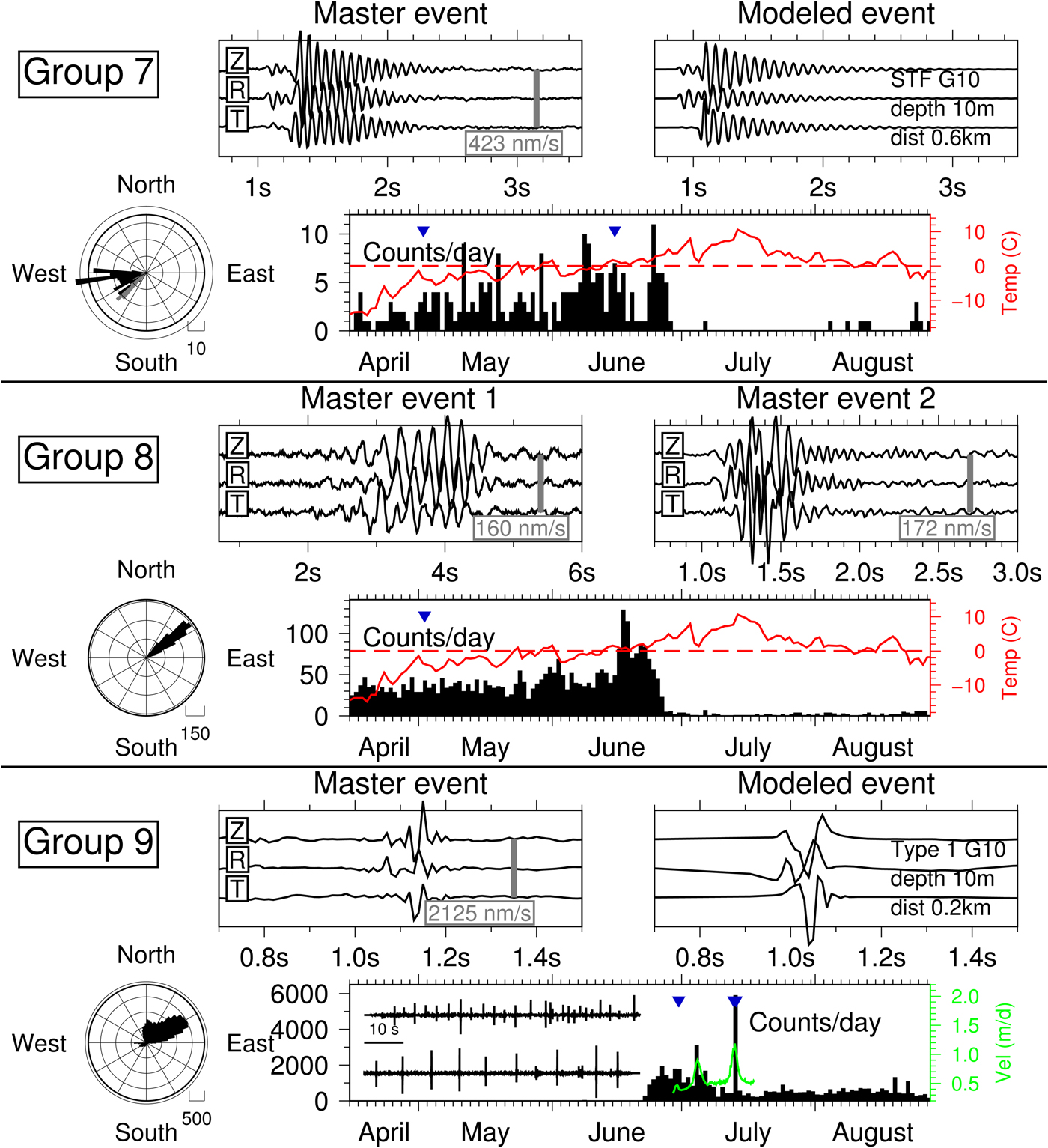
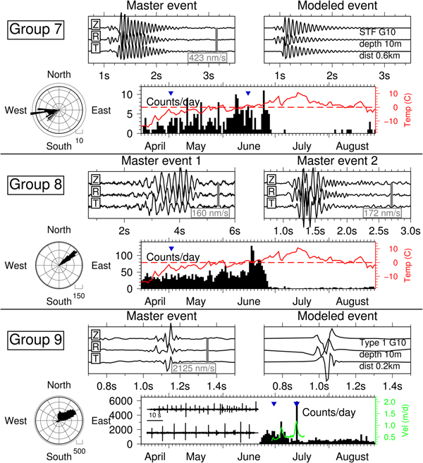
Fig. 7. Icequakes observed at HDF in groups 7–9. See explanation in caption of Fig. 5. For group 8 a second master event is shown instead of the modeled signal. For group 7 a harmonic source time function (STF) is used for seismic modeling (see text). For group 9 an extra inset shows two seismograms of 70 second length each with events during fast-flow episode on 13 July.
Events in group 4 and 5 (Fig. 6) originate from upstream the glacier, but from different distances. Signals of both groups exhibit weak and emergent P onsets, strong, harmonic coda, less impulsive secondary arrivals and tend to have cigar-shaped envelopes. The temporal distribution is distinct from each other. While group 4 shows peak activity in the end of June similar to groups 1–3 when air temperature becomes positive, no events are detected before the end of June, and detection rate is larger in August, with days of high activity coinciding with temperature maxima and local peaks in runoff. In contrast, group 5 exhibits event episodes in May and detections during the whole month of June. The first activity maximum in June is observed in the beginning of the month with air temperature just above 0 °C. Seismicity decreases again when temperature drops below zero. The second, stronger activity maximum for group 5 is observed when air temperatures begin to stay just above 0 °C, a week before the maximum for groups 1–4 when temperatures remain positive at ~5°–10°.
Master events for groups 1–5 are best modeled using a shallow source (10 m), reproducing the observed predominant Rayleigh wave in the secondary arrivals (elliptic polarization), which is much stronger than the P phase. Furthermore, modeling suggests a shallow seismic low-velocity zone with gradually increasing velocities below the ice surface (10–50 m), possibly related to more fractured ice or firn for signals originating upstream. Finally, source Type 1 corresponding to a tensile opening of a crevasse with perpendicular to sub-parallel orientations with respect to glacier flow direction explains the observations best. However, being restricted by an observation at a single station, a strike-slip along a vertically orientated fault (Type 2) would produce similar signals and cannot be excluded. Deep (basal) origin and source types corresponding to uplift (Type 3) and horizontal slip (Type 4) result in signals that do not resemble the observed signals in these groups (Fig. 4).
Icequake group 6
Azimuthal directions and signal lengths of group-6 events (Fig. 6) indicate an origin at Infantfonna, a tributary glacier of Holtedahlfonna to the south of HDF. The activity is low with ~50 detections per day during the temperature maximum in the end of June. The main activity period with 200 events per day is on 4 July, during a strong rain event and at the same day of a fast-flow event at Holtedahlfonna (see Fig. 2d). However, Fig. 2e shows that these signals with frequencies between 1 and 10 Hz mainly occur during morning hours on 4 July, while the increase in high-frequency seismicity at Holtedahlfonna (group-9 events) are being detected at midday. Signals are also being detected during the second rain event on 13 July and during the air temperature maximum in the end of August. Waveform modeling suggests a shallow Type 1 source similar to groups 1–5.
Icequake groups 7–8
Group 7 (Fig. 7) includes only a few events originating <1 km downstream of HDF. The main activity phase ends just before the June air temperature maximum with 10 events per day. The signals show remarkably harmonic waveforms for P wave and secondary arrivals (12–15 Hz) which modeling could not explain by a propagation path effect in a realistic structure (e.g., a guided wave). We were only able to model them by using the harmonic source-time function introduced above, which had been suggested previously to account for fluid resonance or transport in magmatic, hydrothermal, or glacial conduit systems (Lawrence and Qamar, Reference Lawrence and Qamar1979; Chouet, Reference Chouet1985). This simplified model is supposed to simulate a damped oscillation of the conduit/crack wall. We obtain a reasonable fit using a period of T = 0.075 second and a duration of 2.5 second. Retrograde, elliptic polarization of the secondary arrivals is best explained using a shallow source.
The temporal distribution of group 8 is very similar to group 7 (Fig. 7), however, with more events (30–40 per day) between April and the middle of June, followed by a peak and sudden decrease before air temperatures reach the highest seasonal values. In contrast to group 7, the signals seem to originate from upstream the glacier and exhibit cigar-shaped waveform envelopes without clear P phases. Hence, it is difficult to estimate the source distance. However, signal lengths and dominant frequency content vary strongly (see two master events in Fig. 7) and suggest at least two source areas at different distances.
Icequake group 9
Signals in group 9 (Fig. 7) are not longer than 0.2 second and seem to be under-sampled, i.e., frequency content probably exceeds 50 Hz. This suggests a very close source, <300 m away from the geophone. If the most energetic arrivals are interpreted as Rayleigh waves, back-azimuths would mainly point upstream and to the North of HDF. However, since seismic phase identification is difficult, this estimate might be biased. It is striking that activity phases of this group with 3000--5000 detections per day are mainly during fast-flow episodes of Holtedahlfonna (see also Fig. 2e). Seismicity is also present during temperature maximum in the end of June, which is usually the time of the summer speed-up of the glacier (Schellenberger and others, Reference Schellenberger, Dunse, Kääb, Kohler and Reijmer2015). Furthermore, signals seem to be evenly spaced in time during phases of burst-like activity lasting up to1 hour during these days. The regular inter-event times vary between 1 and 10 second. Signals close in time tend to be more similar, however, large waveform variability is present over the entire activity phases. Therefore, we had to use 10 master events to ensure a high event detection rate in visually inspected data.
Icequake group 10
We visually identified a group of signals with durations between 0.5 and 2 second, mainly during the glacier fast-flow episodes in July (Fig. 8). The main difference from other groups is the more equal amplitudes of the first and later phase arrivals. For a few cases, two phases can be identified which might correspond to P and S wave arrivals. However, some events have multiple and/or indistinguishable phases. Furthermore, group-10 events show no clear Rayleigh waves and strong first onsets. All these characteristics are also observed in the synthetic seismogram for a deep source (Fig. 4). Hence, these signals could represent basal icequakes.

Fig. 8. Examples of group 10-events which have presumably a deep source. Date (YYYMMDD) and time of observation (UTC).
DISCUSSION
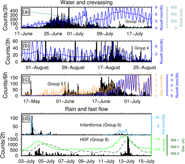
Glaciers are complex systems with multiple, interacting processes, affected by varying external forcings throughout the season. Interpreting the seismic signature of these processes using a single seismic sensor is therefore challenging. Nonetheless, we can at least exclude some processes and present potential alternatives compatible with our own observations as well as previous studies. Figure 9 shows close-ups of the temporal distribution of different icequake groups in interesting time periods together with horizontal glacier velocity, glacier uplift, and modeled runoff, melt, snow cover and precipitation.
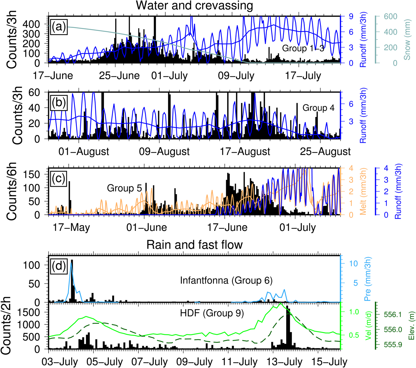
Fig. 9. Close-ups of interesting time periods for different icequake groups and two different source processes. Modeled runoff, snow mass, melt and precipitation in event source areas is given in mm water equivalent. Model outputs with daily and hourly resolution are shown in a–c. Horizontal glacier velocity and elevation are obtained from GNSS measurements.
Surface crevassing and hydrofracturing
Icequakes of groups 1–6 dominate the glacial seismicity at HDF between April and August, except during glacier fast-flow episodes in July. Although seismic signals originate from different source areas up- and downstream of HDF, all groups, except for group 5, share a similar temporal distribution, and all groups can be best modeled using an extensional shallow source that explains the Rayleigh wave-dominated signal as well as the polarity and relative amplitudes on the vertical, radial, and transverse components. We suggest that these signals represent brittle ice failure, i.e, (near-)surface crevasse/crack opening events, as a response to melt and runoff during the early melt season. Our interpretation is consistent with many previous studies that predominantly observed shallow icequakes caused by tensile fracturing of near-surface ice (Neave and Savage, Reference Neave and Savage1970; Deichmann and others, Reference Deichmann2000; Stuart and others, Reference Stuart, Murray, Brisbourne, Styles and Toon2005; Walter and others, Reference Walter2009; Peng and others, Reference Peng2014; Röösli and others, Reference Röösli2014). We cannot resolve the fracture orientation, but comparing modeled and observed signals indicates a range of possible orientations with respect to the event back-azimuth as expected for crevasse fields. A shear motion along a surface fracture would generate similar signals. However, we would expect such sources predominantly along the margins of the glacier which is not supported by the icequake locations indicated by event back-azimuths (Figs 5 and 6).
It is well known that meltwater production has a strong effect on glacial seismicity. Carmichael and others (Reference Carmichael, Pettit, Hoffman, Fountain and Hallet2012) for example found diurnal microseismicity due to thermal bending forces in lake and to a lesser extent in glacial ice during the absence of surface melt, while melt events caused larger, repetitive icequakes related to hydrofracturing. Röösli and others (Reference Röösli2014) found diurnal variation in icequake activity on the Greenland ice sheet caused by surface crevassing presumably depending on meltwater availability. Similarly, our results show an increase of icequake activity in the middle of June coinciding with the gradual increase in modeled runoff (Fig. 9a). However, although temperatures stay above zero and runoff increases further, icequake activity decays in July. Since more runoff would also increasethe seismic noise level, this may be partly explained by a higher detection threshold as discussed above. Another potential explanation is that early in the melt season, water is injected into all cracks leading to hydrofracturing and refreezing. As the melt season progresses, expanse in the hydrofracturing network ensures connection to a runoff path, such that water storage in cracks reduces, resulting in less fracturing despite more water production in the middle of the melt season. The disappearance of the snow pack in the beginning of July (see Fig. 9b and Winsvold and others (Reference Winsvold2018)) might also affect the seismic activity. The general increase in seismicity during the second half of July and August for example (Figs 5 and 9b) might be explained by the direct exposure of the ice surface. However, since runoff and therefore noise level decrease gradually, this can as well be an effect of improved detectability. On the other hand, variations of seismic activity on shorter timescales seem to have a more clear relation to runoff variability. For example, between 31 July and 3 August, as well as between 15 and 21 August (Fig. 9b) seismic activity increases similar as in the end of June. However, it is important to emphasize that the relation between the amount of hydro-fracturing events and runoff is not linear and presumably depends on other glacier conditions such as for example the state of the evolving drainage system as well as glacier flow and strain.
Similar to the diurnality observed by Carmichael and others (Reference Carmichael, Pettit, Hoffman, Fountain and Hallet2012), Podolskiy and others (Reference Podolskiy, Fujita, Sunako, Tsushima and Kayastha2018) reported diurnal variations of glacial seismicity related to large temperature fluctuations and thermal contraction in parts of an Himalayan glacier not protected by debris or thick snow cover. Hence, daily variability in runoff (Röösli and others, Reference Röösli2014) is not the only explanation, and the diurnality in the temporal distribution of STA/LTA detections could also be related to thermal stresses (Fig. 2b). This is supported by the absence of diurnal STA/LTA detections before the middle of July during the presence of sufficient snow cover insulating the ice surface (Fig. 2c and Winsvold and others, Reference Winsvold2018). However, in case of hydrofracturing, diurnal runoff-related fluctuations would also be dampened by potential refreezing and storage of meltwater in the snow pack. Furthermore, groups 1–4 exhibit clear diurnal activity peaks in phase or slightly delayed with respect to runoff also in June and not only in July and August (Figs 9a and b). Hence, we have good evidence that those icequake groups represent most likely hydrofracturing. However, since we do not have glacier flow velocity measurements during the second half of July and August, other processes cannot be excluded.
Group 5 exhibits seismicity earlier and the decay begins earlier than for groups 1–4 (Fig. 6), which seems counter-intuitive since icequakes originate ~4 km upstream, where melt is expected to increase later. However, Fig. 9c shows that there is a relation between seismic activity, melt events, and increase in runoff. Local maxima in meltwater production correlating with seismicity peaks exist in the time periods 14–15 May and 31 May – 3 June. Furthermore, the sudden increase in icequakes on 17 June coincides with the onset of glacier runoff. Finally, on 6 July seismic activity increases together with runoff after a 1–2 day long minimum. Therefore, while triggering of seismic hydrofracturing events clearly depends on meltwater availability, the resulting icequake activity seems to depend also on other so far unknown conditions that can for example make particular areas upstream more sensitive to changes in meltwater production than downstream.
Although the assumption of a 1-D seismic velocity model is probably no longer valid here, seismic waveforms of group-6 events originating at Infantfonna indicate a source process similar to groups 1–5. Since glacier flow velocity is lower than at HDF and the glacier is much smaller in area than Holtedahlfonna, less brittle failure events are observed as expected. The main activity phase on 4 July seems to be a result of a strong rain event which also caused the increase in glacier flow velocity at Holtedahlfonna (Fig. 9d). However, the seismic response of Infantfonna (group 6) and Holtedahlfonna (group 9) to the rain event is different with respect to timing and process (see also Fig. 2e). At Infantfonna rain water seemed to have initiated hydrofracturing close to the surface almost instantaneously, while it took longer at Holtedahlfonna for the discharge to reach the base and to initiate fast flow, which was responsible for another seismic source process which we will discuss later. The delay might exist because melt and rain water travels longer on the surface on Holtedahlfonna than on Infantfonna before it enters the glacier through moulins for example.
Fluid-resonance
Monochromatic signals with a decaying coda like those in group 7 have been observed at glaciers previously and are usually interpreted as being caused by resonance in fluid-filled cracks (Stuart and others, Reference Stuart, Murray, Brisbourne, Styles and Toon2005; West and others, Reference West, Larsen, Truffer, O'Neel and LeBlanc2010). This is in agreement with our modeled seismic signals using a corresponding source-time function (Lawrence and Qamar, Reference Lawrence and Qamar1979). The observations of Stuart and others (Reference Stuart, Murray, Brisbourne, Styles and Toon2005) were made during the surge of Bakaninbreen in southern Svalbard during 9 days in March and April, hence, suggesting the presence of liquid water injected from regions of warm and wet ice during cold meteorological conditions. Likewise, we detect events between April and June. While the absence of those events in July and August may be related to less pressurized liquid water in the system during the melt season due to the opening of more conduits and a more efficient drainage system, we cannot exclude a loss of correlation in the waveforms due to change in the propagation medium, what would prevent detections with the selected master events. The characteristic seismic frequency f 1 of glacial hydraulic fracturing and the quality factor Q, which describes the decay of the coda, can be used to determine the fracture length and fracture width using the method derived by Lipovsky and Dunham (Reference Lipovsky and Dunham2015). A full analysis is beyond the scope of this paper, but using the properties measured from our master event (f 1 = 14.5 Hz, Q=16), we obtain a crack length of ~2 m and width between 2 and 4 mm, which lays within the range of values found previously at different glaciers (see Fig. 7 in Lipovsky and Dunham, Reference Lipovsky and Dunham2015).
Fracturing and settling in firn and snow
Lough and others (Reference Lough, Barcheck, Wiens, Nyblade and Anandakrishnan2015) reported so-called firnquakes with frequency between 1 and 10 Hz that only consist of a dispersive surface wave signal and occur mainly during polar winter in the East Antarctic Ice Sheet. The authors related these signals to formation of macrocracks (crevasses) in the firn caused by thermal contraction during the winter when snow is hard enough to support the buildup of tensile stress that lead to fracturing. While the observation distance was much larger in Antarctica (100–1000 km), the occurrence of group 8 icequakes only before the onset of the melt season, the dominance of surface waves, the lack of earlier seismic phases and the location upstream in direction of the firn area may suggest a similar source process at Holtedahlfonna. The timing fits well with lack of melt and rain before the middle of June as well as observations of Winsvold and others (Reference Winsvold2018), who observed a fast transition from cold and dry conditions in the firn zone to wet-snow conditions above an elevation of 500 m between the middle and the end of June, at the same time as the disappearance of group 8 signals. We, therefore, speculate that static imbalances in the snow and firn may cause sudden settling or fracturing events that emit seismic signals. This seems to occur more frequently during temperature gradients and when air temperature changes between negative and positive degrees, most prominently in the middle of June (see Fig. 7). Since the source distance cannot be constrained, a relation to a firn aquifer discovered 20 km upstream remains unclear (Christianson and others, Reference Christianson, Kohler, Alley, Nuth and Van Pelt2015). Furthermore, even if temporal distributions and source directions are similar for events detected with both master events of group 8, each master event might represent a different process. In fact, the second master event shares some similarities with fluid resonance events in group 7.
Near-surface fracturing during glacier fast-flow
Fast-flow episodes of glaciers are for example caused by strong rain or lake drainage events, and are common at Holtedahlfonna (Bahr, Reference Bahr2015). Glacier uplift is suggested to be caused by high basal water pressure due to increased discharge which facilitates hydraulic jacking and glacier sliding. It is interesting to see a clear seismic signature of the fast-flow episodes on 4 and 14 July (Group 9, Fig. 7). Figure 9d shows that the timing of icequakes correlates well with the increase in horizontal glacier velocity and uplift. Most events occur when horizontal velocity is highest on 4 July. During the second episode icequake activity peaks are more in phase with the largest uplift.
Bursts of near-surface icequakes caused by tensile fracturing during high (dynamic) stress levels have been described for example by Peng and others (Reference Peng2014). Those signals were observed to be very similar, indicating repeated failure at a single source, and exhibited regular inter-event times modulated by passing teleseismic surface waves. However, we do not have indications for passing earthquake signals at the occurrence of group-9 events that could explain why signals at HDF are evenly spaced in time. Regular inter-event times have also been observed for icequakes generated by glacial stick-slip events in Antarctica on different temporal scales (Zoet and others, Reference Zoet, Anandakrishnan, Alley, Nyblade and Wiens2012; Winberry and others, Reference Winberry, Anandakrishnan, Wiens and Alley2013). However, the signal duration of group-9 events and weak P onsets suggest a near-surface origin. Hence, these events are probably not directly caused by basal slip during fast flow events.
Podolskiy and others (Reference Podolskiy2016) showed that tide- or melt-related ice flow variations can cause modulated microseismicity generated by surface crevassing. Strain rate variation due to longitudinal stretching of the glacier was suggested as the source process. Even though no regular inter-event times have been reported, the recorded seismic signals had very similar characteristics compared to our group-9 icequakes considering for example frequency content, duration and the indistinguishable P and S phases. We, therefore, suggest that the stress due to high strain rates during glacier fast-flow events generates bursts of near-surface crevassing icequakes. The regular inter-event times may represent repeated fracturing and stress loading in confined areas close to the geophone (distance <400 m). In contrast to strong crevassing signals in groups 1–6, group-9 signals are not caused by hydrofracturing and are recorded in a closer distance range.
Basal processes
During visual inspection we only found a few events that may originate at the glacier bed (group 10), which confirms previous observations that deep icequakes are rare (e.g. Röösli and others, Reference Röösli2014). The main evidence for a deep source is the absence of a clear Rayleigh wave and more dominant P wave onsets, waveforms that can be in parts reproduced by modeled signals (see deep signal in Fig. 4). However, the events show large waveform variability and ambiguous phase arrivals, so that further analysis and continuous detection is difficult without a seismic network. Deep icequakes have been interpreted as being caused by shear faulting (Walter and others, Reference Walter2009), basal tensile crevasse opening/deep brittle fracture (Stuart and others, Reference Stuart, Murray, Brisbourne, Styles and Toon2005; Walter and others, Reference Walter2009) and stick-slip (Helmstetter and others, Reference Helmstetter, Nicolas, Comon and Gay2015b; Röösli and others, Reference Röösli, Helmstetter, Walter and Kissling2016a). Sliding behavior is common at Kronebreen/Holtedahlfonna and is primarily influenced by water input variability affecting basal friction (Vallot and others, Reference Vallot2017), with subglacial drainage having pulse-like character (How and others, Reference How2017). Furthermore, it has been shown that the efficiency of the drainage system and location of water storage regions have a strong effect on long-term changes in ice flow at Kronebreen (How and others, Reference How2017). Further analysis of the spatial-temporal distribution of group 9 and 10 signals, which occur predominantly during glacier fast-flow events, may therefore help to better understand these processes.
Seismic noise and meltwater
We interpret seismic background noise between 2 and 10 Hz as mainly representing meltwater tremors as observed previously on different glaciers and ice sheets (Röösli and others, Reference Röösli2014, Reference Röösli, Walter, Ampuero and Kissling2016b; Bartholomaus and others, Reference Bartholomaus2015; Helmstetter and others, Reference Helmstetter, Moreau, Nicolas, Comon and Gay2015a). Meltwater production is highest during midday when the ice is most exposed to sunlight (see modeled runoff in Fig. 2a), which roughly correlates with maximum noise amplitudes at HDF. This would also explain the absence of noise diurnality before the snow cover disappeared in the middle of July (Fig. 2c). The time lag with respect to runoff, both on daily (Fig. 2c, 1–2 days delay) and hourly timescales (Fig. 2a, 0–6 hours delay), can be explained by dominant upstream contributions to the supra-, en- and/or subglacial discharge reaching HDF delayed in time. We may speculate that the absence of a delay between runoff and seismic event detections is caused by more channelized upstream runoff contribution which does not lead to increased hydro-fracturing around the sensor in contrast to local runoff. Even though it is present in the modeled runoff, diurnality disappears in the seismic noise for at least 3 days during the rainy time period between 28 and 31 July. Although diurnal meltwater production dominates the runoff signal, seismic noise in that time period is presumably mainly generated by rain drop impacts and/or supraglacial rain water discharge due to the proximity of the geophone to the ice surface. For the same reason, supraglacial meltwater discharge may contribute more to the seismic noise level during the entire melt season than subglacial flow. However, a seismic network is required to validate this hypothesis by locating dominant noise sources. While supraglacial channels are located over the entire glacier surface surrounding HDF, the crevasse field downstream of HDF and a glacier lake north of HDF (Fig. 1a) could represent such sources.
CONCLUSIONS
We have used a single three-component seismic station deployed on an Arctic glacier to investigate the seasonal glacial seismicity. Automatic detection using a STA/LTA trigger revealed a vast amount of icequakes with complex temporal distribution at Holtedahlfonna, Svalbard, between April and August 2016. We grouped visually-observed icequakes and used master event cross-correlation to detect similar signals in the record. Through polarization analysis, seismic waveform modeling, analysis of the temporal distribution, and comparison with previous studies, we concluded that the following glacial processes are presumably responsible for the observed signal categories, with meltwater availability being a crucial parameter for most of them:
1. Near-surface crevasse opening through hydrofracturing is the dominant process generating icequakes at Holtedahlfonna (groups 1–6). Monitoring this type of cryo-seismicity can help to better understand the seasonal evolution of glacier hydrology.
2. Near-surface crevassing due to high strain rates during glacier fast-flow episodes generates bursts of high-frequency icequakes (group 9) which may help to detect and better understand glacier speed-ups as well as the related glacier deformation.
3. Resonance in water-filled cracks is most likely the cause of a few events mainly observed in spring (group 7). These icequakes can be used to estimate the dimension of glacial fractures and potentially their spatial distribution.
4. Fracturing or settling events in dry firn or snow are possible sources for a group of icequakes observed from April until June (group 8). These observations may help to determine the timing of changes in conditions in the firn area with high temporal resolution.
5. Basal processes may be responsible for a few deep icequakes that can help to infer changing conditions at the glacier bed (group 10).
6. Meltwater discharge correlates with seismic background noise and thus can be used to better understand glacial hydrology at Holtedahlfonna.
The presence of seismic observations at a single sensor is in many cases not sufficient for a complete seismological analysis, but represents a rather common situation when we need to analyze local seismicity that is only observed at the closest station of a sparse network. To perform standard and advanced methods on glaciers and ice sheets, such as high-resolution hypocenter location including a good depth resolution, magnitude estimation, moment tensor inversion (e.g. Walter and others, Reference Walter2009), source process modeling (e.g. Lipovsky and Dunham, Reference Lipovsky and Dunham2016) and seismic noise interferometry (Preiswerk and Walter, Reference Preiswerk and Walter2018), there is a clear need for on-ice seismic networks. A seismic network deployment on Holtedahlfonna would allow us to analyze each of our observed signal category in more detail and to better understand the spatial distribution of meltwater noise sources. Nevertheless, our results show that through automatic detection, polarization analysis and waveform modeling, we can still obtain a good overview and characterization of potential cryo-seismic sources, and can draw reasonable conclusions. Furthermore, we recorded high-quality data with low noise level, despite using a simple and cheap instrumental setup with a geophone frozen into a shallow borehole. Moreover, single-station methods utilizing the ambient seismic noise wavefield, such as the HVSR method that we use here, can help to constrain a sub-surface seismic velocity model required for waveform modeling. Hence, if for logistical or financial reasons a network deployment is not feasible, our results strongly suggest that improving understanding of glacier dynamics and hydrology can benefit even from a single seismic station deployment as a complementary method for glacier monitoring allowing for detection and categorization of icequakes and meltwater tremors.
ACKNOWLEDGMENTS
This study was financed by the Norwegian Research Council funded CalvingSEIS (244196/E10) project. VM acknowledges support from the Research Council of Norway through its Centers of Excellence funding scheme, Project Number 223272. CN acknowledges support from ERC-ICEMass. The seismic data logger was provided by the Geophysical Instrument Pool (GIPP) of GFZ Potsdam, Germany. The seismic record of the temporary network stations will become freely accessible through GIPP after 1 October 2020 (http://gipp.gfz-potsdam.de/webapp/projects/view/536). We thank Christian Weidle for organizing instrument rental from GIPP and shipping the data logger to Svalbard. Special thanks go to Cesar Deschamps-Berger for helping during instrument deployment. We used ObsPy (Beyreuther and others, Reference Beyreuther2010) for seismic data analysis. The cross-correlation detector was implemented by Holland (Reference Holland2013). Figures were produced using GMT (Wessel and Smith, Reference Wessel and Smith1998). HVSRs were computed using Geopsy (http://www.Geopsy.org). We thank Antonio Garcia Jerez for providing us with the HV-Inv software to invert HVSRs using the diffuse wavefield theory. Copernicus Sentinel data from 2016 was used in Fig. 1. We thank Evgeny Podolskiy and Timothy Bartholomaus for reviewing the manuscript.


 Open access