


Introduction
Reconstructions of past changes in the thickness and extent of the Antarctic ice sheet are important for understanding past and present sea-level change, and for validating numerical models, necessary to make realistic predictions of changes under future possible environmental conditions. Direct observations of ice-sheet history from satellite data extend back until the 1970s; obtaining longer records requires the use of geologic and glaciological data. For example, radar-detected layers and dated ice cores have been used to infer changes in ice thickness through the Holocene (e.g. Reference Conway, Hall, Denton, Gades and WaddingtonConway and others, 1999; Reference WaddingtonWaddington and others, 2005; Reference Price, Conway and WaddingtonPrice and others, 2007). Marine geologic data have been used to infer ice-margin positions and the presence or absence of ice shelves during the Last Glacial Maximum (LGM) (e.g. Reference DomackDomack and others, 2005; Reference Hillenbrand, Melles, Kuhn and LarterHillenbrand and others, 2012; Reference Stolldorf, Schenke and AndersonStolldorf and others, 2012). Terrestrial geologic data, including drift sheets and moraines deposited by outlet glaciers, have also provided important constraints on past ice thickness. Mapping of these deposits is especially valuable when they can be dated by radiocarbon or cosmogenic-nuclide exposure methods (e.g. Reference Bockheim, Wilson, Denton, Anderson and StuiverBockheim and others, 1989; Reference HallHall, 2009; Reference BentleyBentley and others, 2010; Reference Bromley, Hall, Stone and ConwayBromley and others, 2012; Reference Whitehouse, Bentley and Le BrocqWhitehouse and others, 2012). Radar has also been used to locate past ice-stream margin positions (Reference Catania, Scambos, Conway and RaymondCatania and others, 2006), define boundaries between flow elements (e.g. Reference KingKing, 2009) and, when combined with surface ice-flow velocities and accumulation rates, estimate ages of buried unconformities (e.g. Reference CampbellCampbell and others, 2012) and infer differences in accumulation rates (e.g. Reference Arcone, Jacobel and HamiltonArcone and others, 2012).
In recent years, cosmogenic-nuclide exposure dating methods (Reference Gosse and PhillipsGosse and Phillips, 2001; Reference DunaiDunai, 2010; Reference BalcoBalco, 2011) have been used to date glacial deposits in Antarctica (e.g. Reference StoneStone and others, 2003; Reference Todd, Stone, Conway, Hall and BromleyTodd and others, 2010). Measurements of trace nuclides produced by cosmic-ray bombardment of rock surfaces are used to determine the exposure age of the surface. Although this technique has been used to reconstruct the overall pattern of LGM-to-present ice-sheet thinning in Antarctica, it has several limitations: (1) measurement precision decreases at low nuclide concentrations, so exposure ages from sites that have been exposed for less than ∼1000 years can be subject to large uncertainty; (2) when ice surface-elevation changes are not monotonic, i.e. ice-sheet thinning is interrupted or followed by thickening, exposure-age records are ambiguous; (3) exposure ages of samples collected from outcrops may reflect changes in local rather than regional flow, because the pattern of flow around outcrops is typically complex.
Here we evaluate the hypothesis that the internal stratigraphy of ice adjacent to nunataks contains information about changes in ice surface elevation and flow dynamics over the past hundreds to thousands of years. Subsurface and exposed nunataks affect ice flow and surface mass balance as the ice thickness changes. For example, ice will flow around rather than over a topographic obstacle as it emerges through the ice sheet, and protruding nunataks influence patterns of snow transport by wind, resulting in localized areas of accumulation and ablation. Such changes would be evident in the radar-detected stratigraphy. Following this reasoning, information from patterns of shallow stratigraphy near nunataks should help interpret exposure-age records of ice surface-elevation change over the past millennia. Also, interpretation of local shallow stratigraphy may provide insight into similarities or differences in local vs regional accumulation and flow patterns, which is useful for regional extrapolation of exposure-age data.
We pursue this idea by conducting an ice-penetrating radar study of the shallow (0–400 m) firn and ice surrounding the Schmidt Hills, Pensacola Mountains, Antarctica. We also measured surface ice-flow velocity and accumulation rate to help interpret the radar data. We show that the shallow-ice stratigraphy around these nunataks: (1) is complex; (2) reflects the interplay of through-flowing ice associated with the adjacent Childs Glacier/Foundation Ice Stream and locally sourced ice derived from alpine glaciers; and (3) displays features that may reflect change in the surface elevation of the ice stream.
Foundation Ice Stream and the Schmidt Hills
Foundation Ice Stream (FIS) is the southernmost ice stream that flows into the Ronne-Filchner Ice Shelf in the Weddell Sea Embayment. The catchment of FIS (∼566 000km2) consists of ice originating from both East and West Antarctica (Reference Joughin and BamberJoughin and Bamber, 2005; Reference Rignot, Mouginot and ScheuchlRignot and others, 2011). Thus, thickness and velocity changes in the lower FIS will contain a record of changes in both regions. The Schmidt Hills are a group of nunataks situated near the eastern edge of FIS as it enters the Filchner Trough embayment (Fig. 1) ∼ 4 0 km downstream of the currently estimated grounding line (SCAR, 2012). The hills are approximately 27 km long and 12 km wide, with nunatak elevations reaching >700m above the current ice surface. Childs Glacier drains from the southern boundary of the Schmidt Hills and turns north to merge into the eastern edge of FIS. Other small valley glaciers originating within the Schmidt Hills flow westward into Childs Glacier and FIS.
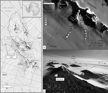
Fig. 1. Locator maps of the Schmidt Hills and Foundation Ice Stream showing: (a) elevations from the RADARSAT-1 Antarctic Mapping Project (RAMP) digital elevation model (DEM), the current grounding-line interpretation from the Antarctic Digital Database (ADD) and the location of the Schmidt Hills in the Pensacola Mountains relative to FIS and Ronne–Filchner Ice Shelf; (b) QuickBird 0.6 m pixel resolution satellite image of the Schmidt Hills showing location of the Childs Glacier/FIS flow relative to GPR profiles 1–4 (white solid lines, L1–L4), GPR profiles collected but not imaged (white dashed lines), surface ice-flow velocities (black arrows, underlined lettering; m a–1), the meltwater pond near line 2 (MW), blue-ice areas (BIA), accumulation rates (circles; cm a–1) and the location of the photo shown as (c) (white arrow, P); and (c) photo with approximate radar profile locations (dotted lines; L1–L4), the shear margin and FIS with dotted arrow pointing towards the Ronne–Filchner Ice Shelf. Imagery #2012 DigitalGlobe, Inc.
Reference Graf, Reinwarth, Oerter, Mayer and LambrechtGraf and others (1999) collected firn cores along a traverse up FIS; these cores show a regional pattern of increasing accumulation rate from the FIS grounding line to the north toward the ice-shelf edge. They estimated a 10.1 ± 3 . 0 cm w.e. a- 1 average accumulation rate between 1947 and 1994 at their core closest to the Schmidt Hills, ∼20 km from the end of our ground-penetrating radar (GPR) profile 1 (L1 in Fig. 1b). Reference Joughin and BamberJoughin and Bamber (2005) used regionally derived elevation and velocity data to estimate regional mass balance through a flux-gate method. They estimated a positive mass balance (+2.0 ± 1 . 1 cm w.e. a-1) for the FIS catchment. The currently mapped grounding line of FIS is ∼ 4 0 km up-glacier of the Schmidt Hills (Reference Rignot, Mouginot and ScheuchlRignot and others, 2011; SCAR, 2012), placing the floating shelf in front of the Schmidt Hills. The implication is that grounding-line changes have likely been an important control on Holocene changes in the configuration and thickness of FIS adjacent to the Schmidt Hills (e.g. Reference Conway, Hall, Denton, Gades and WaddingtonConway and others, 1999). Grounding-line advance and retreat would cause, respectively, thickening and thinning of FIS at this location (e.g. Reference Goldberg, Holland and SchoofGoldberg and others, 2009). Absent significant changes in local accumulation rates, this would also cause thickening or thinning of local glaciers in the Schmidt Hills.
Finally, the complex topography of the Schmidt Hills influences local snow accumulation and ablation. Sastrugi directions and the pattern of snow accumulation indicate that prevailing winds are from the east, perpendicular to the long axis of the Schmidt Hills towards FIS. This results in small pockets of firn-sastrugi (< 3 - 4m depth) occasionally overlying the scoured and exposed blue ice within the Schmidt Hills valleys, where winds are more confined (e.g. Reference BintanjaBintanja, 1999). In contrast, accumulation zones are situated near the mouth of each valley, where winds are not as confined.
Data Collection and Processing
During December–January 2010–11 we profiled stratigraphy and ice depths of the valley glaciers in the Schmidt Hills and the fringe icefields between the Schmidt Hills and Childs Glacier/FIS. We used a Geophysical Survey Systems Inc. (GSSI) SIR-3000 control unit and model 3107 100 MHz monostatic transceiver. The four radar transects we discuss here were collected perpendicular to the long axis of the Schmidt Hills towards Childs Glacier/FIS (Figs 2–5). The antenna was oriented perpendicular to profile direction, and the unit was towed via snowmobile at approximately 3–7 km h–1. Profile traces were recorded for 4000–6300 ns with 2048–4096 16-bit samples per trace for deep applications, and 100–400 ns at 2048 samples per trace for shallow applications. Approximately 8–16 traces s–1 were recorded, translating to 4–20 scans m–1 depending on tow speed. Lower profiling speeds were employed for deeper ice to ensure improved stacking capabilities. Profiles were recorded with range gain and post-processed with bandpass filtering to reduce noise. We applied distance and elevation corrections using regularly spaced 50 m GPS recording, and simultaneously recorded GPR distance markers with kinematic GPS survey data using a Trimble 5700 control unit and Zephyr Geodetic antenna. GPR post-processing also included stacking to increase the signal-to-noise ratio. Radar profiles were collected over both blue ice and firn. We used a relative permittivity of 3.0 (0.173m ns–1 wave velocity) to convert two-way travel time (TWTT) to depth for figures showing blue ice and firn and in full ice-depth profiles (Figs 2a and b, 3a, 4a–c and 5a). This slightly lower value provides some amount of correction for lower-permittivity firn overlying the higher-permittivity ice. A relative permittivity of 2.4 (0.189 mns–1 wave velocity) was used for figures which primarily image firn (Figs 2c, 3b, 4d and 5b).
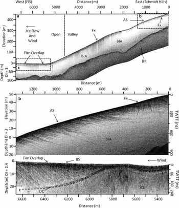
Fig. 2. Line 1 (L1) 100 MHz GPR profile. (a) Elevation-corrected full depth profile with labels for bedrock (BR), blue-ice areas (BIA), an ablation surface (AS), surface tensional ice fractures (Fx) and the approximate division between confined (valley) and unconfined (Open) ice flow. Depth is based on a dielectric permittivity (DI) of 3.0 and two-way travel time (TWTT). (b) Zoom from (a) showing detail of dipping stratigraphy in the BIA, AS and hyperbolas caused by the Fx. (c) Zoom from (a) showing detail of the firn overlap described as wind-deposited bedding sequences (BS), buried-firn–blue-ice unconformity (UC) and the ice beneath the UC which lacks internal stratigraphy.
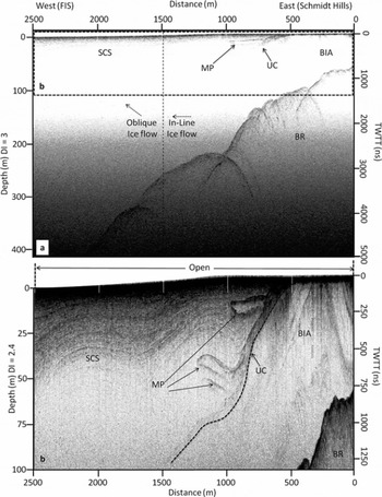
Fig. 3. Line 2 (L2) 100 MHz GPR profile. (a) Elevation-corrected full depth profile with labels for bedrock (BR), blue-ice areas (BIA), surface-conformable firn stratigraphy (SCS), an unconformity between the BIA and SCS (UC), interpreted refrozen melt ponds (MP), and region of the transect which resides in line with surface ice-flow velocity measurements (‘In Line’, 0–1500 m) relative to the region oriented oblique to the surface ice-flow velocities (‘Oblique’, 1500–2500 m). Depth is based on a dielectric permitivity (DI) of 3.0 and TWTT. (b) Zoom from (a) showing detail of BIA relative to the UC, a series of three refrozen melt ponds (MP) and the abutting SCS with depth scale based on a DI of firn (DI = 2.4).
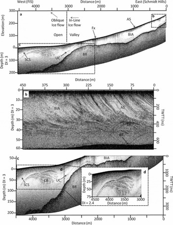
Fig. 4. Line 3 (L3) 100 MHz GPR profile. (a) Elevation-corrected full depth profile with labels for bedrock (BR), blue-ice areas (BIA), an ablation surface (AS) surface-conformable firn stratigraphy (SCS), an unconformity between the BIA and SCS (UC), and region of the transect which resides within the valley and in line with surface ice-flow velocity measurements (‘In-Line’, 0–3000 m) relative to the region which has exited the valley (‘Open’) and is oriented oblique to the measured surface ice-flow velocities (‘Oblique’, 3000–4600 m). Depth scale is based on a dielectric permitivity (DI) of 3.0 and TWTT. (b) Zoom from (a) showing detail of BIA which includes the AS and complex reflections (CR) above BR. (c) Zoom from (a) showing detail of SCS overlying potential cross-bedding (CV) or relict bedding planes and a blue-ice unconformity (UC) above BR. (d) Zoom from (c) showing potential relict cross-bedding in greater detail.

Fig. 5. Line 4 (L4) 100 MHz GPR profile. (a) Elevation-corrected full depth profile with labels for interpreted bedrock (BR, dashed line) and side reflections. Depth scale is based on a dielectric permitivity (DI) of 3.0 and TWTT. (b) Zoom of shallow features from (a) showing surface-conformable firn stratigraphy (SCS) overlying an unconformity (UC) and a reflection-free region below the UC which we interpret as being blue ice (ICE).
In December 2010 we placed eighteen 2 m long wooden ablation stakes (Fig. 1b) along radar profiles 2 (Fig. 3) and 3 (Fig. 4), at 250–500 m increments from each other, to determine local mass balance and surface ice-flow velocities. The stakes were placed by drilling holes into the firn or ice with a hand auger; ∼ 1 m of the stake extended above the surface. Prior to stake insertion, the hole locations were recorded using rapid-static surveys with two Trimble 5700 GPS receivers and Zephyr Geodetic antennas. One unit was used as a temporary base station on a nearby rock outcrop. The unit was used to measure the location of each stake hole. Stakes were resurveyed in December 2011 (375-377 days later) to determine mass balance and surface ice-flow velocities. The Canadian Spatial Reference System was used to geolocate the base stations. Mean uncertainty in the velocity components calculated over the 1.03 year interval is 0.04 m a- 1.
Data Description
We discuss four GPR profiles originating from the Schmidt Hills and terminating at the shear zone of Childs Glacier/FIS (Fig. 1b). Two profiles (1 and 3; Figs 2 and 4) were collected over glaciers that originate within valley cirques that merge into Childs Glacier, and two profiles (2 and 4; Figs 3 and 5) were situated immediately adjacent to nunataks closer to Childs Glacier/FIS (i.e. not originating within valley cirques). Each profile was collected approximately along the flowline within the valleys or when close to the nunataks, but our surface ice-flow velocity data imply that the radar profiles diverged from the flow direction as we approached the shear margin.
Profile 1 (Fig. 2)
This 6750 m long valley-glacier profile starts at 228 ma.s.l. in Nervo Valley and ends at 202m a.s.l. near the shear margin of Childs Glacier/FIS (L1 in Fig. 1b and c; Fig. 2a). Of the profiles collected, this is the most northerly and closest to the Ronne–Filchner Ice Shelf (Fig. 1a). The majority of the profile is within a topographically confined valley glacier; however, from 4500 to 6750 m the glacier is not valley-confined and is close to the same elevation as Childs Glacier/FIS (Fig. 2a). Ice-flow direction in this lower section of the glacier is likely influenced by FIS flow. A strong bedrock reflection at depths of 100-200 m is visible throughout the profile (Fig. 2a). From 0 to 1400 m (within Nervo Valley) the glacier consists of blue ice (BIA in Fig. 2b) with steeply dipping internal horizons (10-208 apparent dip towards the Schmidt Hills) beginning at depths of >60 m and truncated at the present ablation surface (AS in Fig 2b). The thickness of some of these internal layers increases with depth. Thin extensional fractures <0.5 m wide (Fig. 2a and b; Fx) were also evident on the blue-ice surface in the field from 0 to 1400 m and 2500 to 4000 m along the transect, resulting in visible hyperbolas in the unmigrated radar record. At ∼5300m the exposed blue ice is overlapped by firn, and from 5300 to 6750 m only firn was observed at the surface in the field. The radar profile shows this firn contains shallow-dipping parallel internal horizons (∼108 apparent dip towards the Schmidt Hills), which terminate at the surface (BS in Fig. 2c), and an unconformity that undulates between 2 and 20 m depth (UC, dashed line in Fig. 2c). Internal stratigraphy is not visible below the unconformity.
Profile 2 (Fig. 3)
This 2500m profile starts ∼100-200m from a nunatak situated between Mount Nervo and Mount Coulter in the Schmidt Hills (L2 in Fig. 1b and c). Elevations range from 183 ma.s.l. near the nunatak to 175ma.s.l. at the Childs Glacier/FIS shear margin. To the west of the nunatak and <50m north of the radar profile, meltwater derived from runoff from the nunatak had formed a small lake on the ice surface (MW in Fig 1b; Fig 3b, ∼0-500m). In some places near the edge, the lake was at least 1 m deep. We observed surface-exposed blue ice from 0 to 700 m (BIA in Figs 1b and 3b) under and to the south of the radar profile, and firn covering the surface between 700 and 2500 m. The profile shows ice thickness increasing from 75 m near the nunatak to >420 m (the depth limit permitted by this GPR configuration) near the shear margin (BR in Fig. 3a and b). The bed exhibits several benches intermixed with bowtie reflections and steeper topography, suggesting that a series of small overdeepenings might exist between each sub-horizontal bench. Migration of the radar data supports the interpretation of benches centered at 1100, 1600 and 2000 m but does not reveal any overdeepenings. In the shallower subsurface near the nunatak between 0 and 700 m, the profile shows steeply dipping blue-ice stratigraphy terminating at the surface (BIA in Fig. 3a and b). An unconformity that dips steeply to the west separates this unit from an overlying unit of surface-conformable firn stratigraphy (SCS in Fig. 3a and b). The surface-conformable stratigraphy (SCS) is visible to 55 m depth from 700 to 2500 m. Adjacent to the unconformity (UC in Fig. 3a and b), we observed unusual several-meter-thick units bounded by strong sub-horizontal reflections but with no internal stratigraphy (MP in Fig. 3a and b). These units are sub-parallel to the SCS but appear locally unconformable (MP in Fig. 3b).
Profile 3 (Fig. 4)
This profile traverses ∼9000m (L3, solid and dotted white line in Fig. 1a and b) from a cirque situated between Mount Coulter and an unnamed nunatak located to the northwest. We only show the first 4500 m of this profile that is proximal to the Schmidt Hills in the figures (L3, solid line in Fig. 1b; Fig. 4) because it has the most structural complexity. The remaining section that approaches the shear margin has relatively simple SCS and bedrock depths greater than the maximum range of our GPR system, precluding any significant interpretation. The profile starts at 525 ma.s.l. within the valley and ends at 181 m a.s.l. near the shear margin. The upper valley surface (0-2600m) consisted of a mix of exposed blue ice or thin pockets of wind drift and firn (&≤0.5 m thick) covering the ice (BIA in Figs 1b and 4a and b). At ∼2500-9000 m the surface appeared to be completely covered with firn once the glacier departed the valley confines (‘Open’ in Fig 4a). Ice depths range between 75 and 200 m in the portion of the profile shown in Figure 4 (BR in Fig. 4a). A ∼100 m deep basin occurs at 1300 m followed by thinning to only 50 m before ice exits the valley. Outside the valley confines, the ice depth increases rapidly to >400m while approaching the shear margin, similar to profile 2. The bedrock topography also exhibits a similar series of steps and benches to that in profile 2. The shallow subsurface between 0 and 1000 m exhibits steeply dipping (∼20° apparent dip towards the Schmidt Hills) blue-ice stratigraphy that tapers to near-horizontal layers intermixed with complex reflections near 40 m depth (CR in Fig. 4b). These layers are truncated at the blue-ice surface (AS in Fig. 4b). Between 2000 and 3000 m, surface cracks &≤0.5 m wide were visible in the field. These surface crevasses are related to increased noise and hyperbolic reflections in the radar profile (Fx in Fig. 4a). Continuous internal stratigraphy is not present in this blue-ice region. From 2600 to 6800 m a continuous upper SCS firn unit thickens from 0 to 75 m, initially overriding the blue ice of the valley glacier, resulting in a faint unconformity (UC in Fig. 4a and c). This unconformity fades between 2800 and 3200 m and is replaced at 3200-4400 m by a series of complex horizons that resemble cross-bedded layers at 25-75 m depth. The upper SCS firn layers conform to the top horizon of these cross-beds as opposed to terminating (CB in Fig. 4c and d). Stratigraphy is not evident below the potential cross-beds.
Profile 4 (Fig. 5)
Profile 4 is an 8000m long transect covering a relatively small elevation range between the Schmidt Hills and the FIS shear margin (250-173 ma.s.l., respectively (L4, solid and dashed line in Fig. 1b)). The entire profile was collected over firn, and the western 5 km was simple SCS with bedrock too deep to image, so we show only the eastern 3 km in figures (Fig. 5a). Ice thickness is ∼200m near the Schmidt Hills; however, the bedrock reflection (BR, dashed line in Fig. 5a) is faint and disappears at 750m distance along the profile, suggesting that the bed dips steeply and ice thickens quickly toward the shear margin. Faint side reflections also suggest complex bed topography. The surface unit in this profile is SCS throughout the length of the transect (SCS in Fig. 5a and b). However, between 0 and 1000 m the SCS overlies and terminates at a prominent unconformity (UC in Fig. 5b) at 20-60 m depth. The SCS horizons dip towards the Schmidt Hills at this termination. No stratification is visible below the unconformity.
Ablation-velocity stakes
One-year measurements of accumulation (Fig. 1b, circles) and surface ice-flow velocities (Fig. 1b, arrows) were collected along profiles 2 and 3. Accumulation rate measurements range from -5 ± 2 cm a - 1 within the upper ablation zone of the valley glacier (L3 in Fig. 1b) or near the nunatak on profile 2 (L2 in Fig. 1b) to 9 ± 2 cm a- 1 proximal to the Childs Glacier/FIS shear margin. The pattern is complex; for example, a pocket of ablation occurs within the Mount Coulter valley in profile 3, but upstream and down-glacier of this pocket a positive mass balance prevails. Surface ice-flow velocities range from as low as 0.04 ± 0.04 m a- 1 to 0.63 ± 0.04 m a- 1 . The vectors suggest a trend parallel to GPR profile 2 from 0 to 1500 m (L2 and arrows in Fig 1b; ‘In-Line’ and ‘Oblique’ ice flow in Fig. 3a) and from 0 to 3200 m for GPR profile 3 (L3 and arrows in Fig 1b; ‘In-Line’ and ‘Oblique’ ice flow in Fig. 4a) before diverging to the northwest. Note that caution is needed because the estimates of accumulation and surface velocity are derived from measurements spaced only 1 year apart.
Interpretation and Discussion
Observed radar-detected stratigraphy includes: (1) blue ice with internal stratigraphy; (2) blue ice that lacks internal stratigraphy; (3) surface-conformable firn stratigraphy (SCS); and (4) firn that exhibits complex bedding sequences (CB). These stratigraphic features represent a transition zone from local to regional weather patterns and ice-flow dynamics. We interpret the sequences of surface-conformable firn that show progressive overlap of underlying blue ice (L2-L4 in Fig. 2b; SCS in Figs 3b, 4b and 5b) as reflecting accumulation of firn on top of ice derived from Schmidt Hills glaciers, as this ice flows into accumulation zones in more open topography away from the hills. This contrasts with the firn that exhibits more complex bedding sequences (L1 in Fig. 1b; BS in Fig. 2c; CB in Fig. 4c and d), which is likely a result of accumulation and ablation caused by local topographic influences. The change in flow direction as the valley glaciers exit the Schmidt Hills valleys may further complicate the stratigraphic record as ice flows through successive accumulation and ablation regions.
Blue-ice areas (BIA)
The Schmidt Hills create complex local weather patterns resulting in steep wind exposure and snow accumulation gradients (e.g. Reference BintanjaBintanja, 1999). BIAs are prevalent in the Schmidt Hills (Fig. 6); BIAs evident in radar-detected stratigraphy along profiles 1 (L2 in Fig. 1b; BIA in Fig. 2a) and 3 (L3 in Fig. 1b; BIA in Fig. 4a) are caused by confined valley-winds; BIAs evident along profile 2 (L2 in Fig. 1b; BIA in Fig. 3b) are likely caused by topographic blocking.

Fig. 6. Block diagram showing regional and local dynamics that contribute to radar stratigraphy surrounding the Schmidt Hills. Regional dynamics include climate variability and ice-sheet mass balance (positive or negative), grounding-line changes (advance or retreat) resulting in associated changes in ice-flow velocities (black arrows), and ice-stream thicknesses which can alter buttressing and associated flow responses upstream and adjacent to FIS. Local dynamics include a lowering of the surface (which was originally regionally controlled) causing a change from previous ice-flow directions over topographic obstructions to current ice flow around these obstructions, a change in dominant katabatic wind patterns resulting in localized ablation and blue-ice areas (BIA) within valleys, and localized pockets of accumulation as either bedding sequences (BS) or through overlap of firn onto BIAs. Surface velocities, accumulation rates and radar stratigraphy provide estimates of positive or negative surface elevation changes relative to the combined dynamical processes.
Complex bedding sequences and surface-conformable stratigraphy
In profile 1 we interpret the dipping firn stratigraphy (‘Firn Overlap’ in Fig. 2c) as being a local bedding sequence similar to larger regional depositional features that form on windward slopes (e.g. Reference Arcone, Jacobel and HamiltonArcone and others, 2012). In this case, it is likely that increased wind speed caused by the local confining topography of Nervo Valley scours the upper glacier and deposits snow down-glacier where wind speeds decrease due to the lack of confining topography (BIA, ‘Local Accumulation’ and BS in Fig. 6). Note that the slight surface elevation rise approaching the FIS shear margin (Fig. 2c, 5800–6750 m), enhances this process (Reference Frezzotti, Gandolfi and UrbiniFrezzotti and others, 2002). In contrast to prograding bedding sequences, profiles 2–4 reveal thick SCS overlapping blue ice. The lack of windward slopes in each of these profiles may preclude the formation of prograding sequences (Reference Frezzotti, Gandolfi and UrbiniFrezzotti and others, 2002). However, the buried cross-beds in profile 3 (Fig. 4c and d) may be relict bedding sequences similar to those in profile 1 that formed up-glacier between 2000 and 3000 m where the topographic bedrock rise exists (BR in Fig. 4a).
Oblique ice flow
An alternative explanation of the bedding sequence observed along profile 1 (Fig. 2c) might be that the transition zone between the Schmidt Hills and the FIS shear margin has a large component of flow that is parallel to the ice stream. In this case, stratigraphic sequences in ice in the transition zone would reflect variations in accumulation and ablation inherited from upstream. Flow stripes visible in satellite imagery (Fig. 1b, QuickBird 0.6m resolution image) and surface ice-flow velocities (Fig. 1b, black arrows) oriented oblique to the long axis of the Schmidt Hills on profiles 1 and 2 suggest this is a plausible cause for the firn bedding sequence in profile 1 (Fig. 2c). In this case, a particular parcel of ice would experience ablation within the ablation zone of a valley glacier, flow out of the Schmidt Hills into a topographically controlled zone of accumulation near the shear margin and then be carried northwestward into another zone of ablation. The sequence of events evident in this stratigraphy could reflect a steady-state flow pattern and would not necessarily require a change in FIS surface elevation. This explanation is consistent with the observation that the upper stratified firn unit of profile 1 is the only truncated firn unit at the present surface of all four profiles collected. These two local scenarios could potentially be resolved with more extensive measurements of modern flow velocity and accumulation rates.
Regional and Local Links
We interpret the unstratified unit below the unconformities present in profiles 2–4 as being ice derived from Schmidt Hills valley glaciers; however, it appears unlikely that the thickness of ice towards the shear margin was entirely derived from valley glaciers, and more likely that this unit includes remotely sourced ice delivered by Childs Glacier/ FIS. We easily imaged the unconformity between the SCS and valley-glacier blue ice. However, we did not observe any additional boundaries at similar or greater depths in the lower unit that might reflect a separation of ice derived from valley glaciers and through-flowing Childs Glacier/FIS ice. If such a boundary does exist, it would imply either (1) the attenuation rate was too great to image the two blue-ice units at buried depths; (2) the two units are intermixed so that they cannot be resolved by the radar system; or (3) the contrast between the two units is below the sensitivity of the radar system. One possibility is that the underlying unstratified ice has undergone significant deformation during flow, resulting in minimal internal strata visible in the radar profiles. In contrast, the overlying firn or ice unit has well-defined stratigraphy due to minimal deformation since time of deposition. We view the question of distinguishing remotely sourced ice associated with FIS from locally derived valley-glacier ice as important to our overall objective of understanding the stratigraphic record of ice surface elevation changes near nunataks. Thus, better imaging of blue ice below the unconformity is an important future challenge in this work. The fact that we did successfully image stratigraphy within some areas of valley-glacier-derived blue ice (Figs 1a, 2 (top) and 3a) suggests that this is possible.
A final note on the blue ice in regard to changing surface elevations is worthy of mention. Preliminary results from cosmogenic-nuclide field sampling efforts suggest that at one time ice flowed over much of the Pensacola Mountains, as opposed to around as is now the case (‘Previous Ice Elevation’ and ‘Previous Ice Flow’ in Fig. 6). In this instance, the deglaciation of the Schmidt Hills resulted in a dramatic change of ice-flow trajectories and it is possible that some ice within the study area represents relict and now stagnant ice that has not yet been evacuated from the valley basins. We suggest that blue ice in the upper reaches of the basin that still exhibits stratigraphy may represent this past overriding ice that has ablated through time following deglaciation of the Schmidt Hills. A more detailed and expansive analysis of ice flow through this region, including an attempt to date different units within the radar stratigraphy, is needed to delineate the potential origins of these structures.
Stratigraphic ages and surface elevation changes
Combined field and radar observations suggest that the underlying unit in profiles 1–4 is blue ice because it is exposed in several locations at the surface where the unconformable horizons begin in each radar profile and these horizons dip away from the surface with continual overlapping of new accumulation over the down-flowing valley ice (Reference Welch and JacobelWelch and Jacobel, 2005). In profiles 2–4, stratigraphy terminates against this unconformity (UC in Figs 3b, 4c and 5b). Reference CampbellCampbell and others (2012) used surface ice-flow velocities and a single accumulation rate to estimate the age of buried radar stratigraphy. Here we use the ice-flow velocities to estimate the horizontal transit time for ice to flow from the beginning of the radar profile proximal to the Schmidt Hills to where the deepest location of the unconformity is located. We selected profile 2 for this calculation because the subsurface structure is relatively simple; SCS overlaps a strongly reflecting and relatively continuous unconformity (UC in Fig. 3b) and the profile was collected parallel to ablation stake surface velocities for the distance in which the unconformity is visible (Fig. 1b, black arrows). Using this approach we calculate that the ice at the maximum depth of the unconformity ( 1 0 5 ± 6 m ; Fig. 2b) is ∼1210 years old.
We also interpret the thick sub-horizontal units attached to the unconformity (MP in Fig. 3a and b) as being past surface melt ponds (i.e. similar to the pond that currently exists) that refroze and were subsequently buried and transported down-glacier. This interpretation is supported by field observations of the current melt pond, and radar measurements that indicate a strong dielectric contrast, appropriate phase polarity shift expected between firn and ice, and a lack of internal stratigraphy within the units (expected due to the prior melt). Three of these features exist; estimated ages at the maximum syncline point for each structure based on measured surface velocities are 150 years BP, 400 years BP and 480 years BP. Uncertainties due to measurement errors are ∼2%, but significantly larger uncertainties are likely because of variations in ice-flow velocities at the surface and with respect to depth as well as accumulation rates over time. However, these ages provide a first-approximation timescale for the radar-stratigraphic features observed.
We use these results with a distance-averaged accumulation rate of 2.8 ± 2 cm a- 1 from the five accumulation stakes placed at equally spaced intervals along the length of profile 2 (L2 in Fig. 1b; circles), as a first approximation to surface elevation change estimates of the Schmidt Hills glaciers. We use a distance-averaged accumulation rate because of the uncertainties associated with our 1 year mass-balance data. If this accumulation rate is representative of the mean value over 1200 years, we estimate that the mass flux out of the glacier relative to the mass flux into the glacier over this time period (determined from velocity vectors over the unconformity of radar profile 2) results in a -3.5 ± 2 m elevation decrease. In conclusion, it appears, to first order, that the ice apron connecting FIS to the Schmidt Hills has a slightly negative mass balance (-0.25 cm a-1) over this time period, implying that the elevation of the ice margin decreased whether or not there was any change in the surface elevation of FIS.
Regional vs local accumulation rates
The regional positive accumulation rate determined from a series of center-line sites on FIS (Reference Graf, Reinwarth, Oerter, Mayer and LambrechtGraf and others, 1999) shows approximate agreement with our short-term accumulation rate estimates. Using an estimated firn density of 0.43gcm- 3 , our most closely located accumulation-ablation stake suggests 9 ± 2 cm w. e. a - 1 relative to the closest firn core extracted by Reference Graf, Reinwarth, Oerter, Mayer and LambrechtGraf and others (1999) that is ∼26km distant (1999; ∼10cmw.e.a– 1 ) . The remaining stakes from our study indicate an increasing trend in accumulation rate from the ablating ice closest to the Schmidt Hills, towards FIS. We recognize the shortcoming of not being able to estimate interannual variability due to the short time period (377 days) from which our accumulation rates are derived. However, the general spatial trend of our data relative to the accumulation rate derived from the nearby site by Reference Graf, Reinwarth, Oerter, Mayer and LambrechtGraf and others (1999) is promising.
Conclusions
Radar-detected stratigraphic relationships indicate the following events: (1) deglaciation of the Schmidt Hills causing changing flow direction around the nunataks; (2) ablation in the upper and central portion of the down-flowing valley glaciers where winds are topographically confined; (3) local mass redistribution of the up-glacier ablated ice resulting in prograding growth of bedding sequences over the blue ice at the transition zone between the Schmidt Hills and FIS; (4) accumulation from regional precipitation causing progressive overlap of surface-conformable firn onto valley glacier blue ice at the transition zone between the Schmidt Hills and FIS. Comparison of radar-detected stratigraphy with velocity and accumulation measurements suggests that the transition zone between the Schmidt Hills and FIS has a slightly negative mass balance, implying a ∼ 3 m decrease in the ice-margin elevation over the past ∼1200 years.
Acknowledgements
We thank Richard Hindmarsh, Gwenn Flowers and two anonymous reviewers for carefully reviewing and improving the manuscript with their feedback. We thank Steven Arcone and John Stone for helpful comments during various stages of the project. We thank Nathan Lamie, Steven Decato and Jesse Stanley (US Army CRREL) for providing technical support prior to and following field seasons, and Robert Hawley and Steven Arcone for providing field equipment. We thank the Polar Geospatial Center for support and access to satellite imagery. Funding for this research was provided by the US National Science Foundation to Conway (ANT-0838783), Balco (ANT-0838784) and Todd (ANT-0838256).


