


Introduction
Because of the significant information crevasses can provide regarding glacier flow dynamics, an increased understanding of their evolution is important. However, crevasse dynamics are difficult to quantify due to numerous variables which affect their formation. Crevasses form when a yield tensile stress or critical strain rate is reached. Early research suggested critical strain rates of 0.01 a–1 are required in extending flow to form surface crevasses in temperate ice (Reference HoldsworthHoldsworth, 1969), while Reference MeierMeier (1958) suggested that crevasses in temperate ice and firn seem to form at lower strain rates than those required in cold firn. Reference Hambrey and MullerHambrey and Muller (1978) found new crevasses opening over strain rates ranging from 0.004 to 0.163 a–1. Other studies (Reference KehleKehle, 1964; Reference VaughanVaughan, 1993) used the concept of a principal stress at the ice surface exceeding a critical value to cause crevasse formation. Consistent with Meier’s suggestion, Reference VaughanVaughan (1993) found that 90–320 kPa are needed to cause crevasses in both cold and temperate glaciers while Reference Forster, Rignot, Isacks and JezekForster and others (1999) found 169–224 kPa are needed in temperate ice. However, Reference VaughanVaughan (1993) found no systematic relationship between firn temperatures and critical stresses, contrary to Reference MeierMeier’s (1958) original suggestion that cold firn or ice has a greater tensile strength than warmer firn and ice. Tensile strength, along with elastic properties of ice, are heavily temperature-dependent; however, Reference VaughanVaughan (1993) suggested that tensile strength also depends on density, bed and surface topography, ice depth, impurities (e.g. water or debris) and crystallography. The range of stresses, strains, nonlinear rheological properties, thermal regimes, geometric boundary conditions and the physical condition of firn and ice challenge the efficacy of crevasse evolution models in complex glaciers. Here we contribute to the published strain-rate estimates required for crevasse formation within polar (cold) glaciers using numerical models constrained by field-measured surface strain rates of a relatively simple glacier.
We consider a small, cold, alpine glacier located high in the Alaska Range, USA. Its extent is well defined, it contains minimal debris and water and it likely exhibits relatively constant annual velocities, alleviating some material property and associated modeling complexities. The lack of debris and water content was determined from observations made during two field seasons that includedshallow firn-core samples collected in 2010 and snow-pit samples collected in 2011 (Reference CampbellCampbell and others, 2012a). Our observations and GPS data confirmed this was an ice divide, while ground-penetrating radar (GPR) profiles revealed minimal deformation within surface-conformable stratigraphy (SCS). Most importantly the GPR profiles revealed buried crevasses at and immediately adjacent to the ice divide, which eliminated the possibility that the crevasses formed up-glacier. In addition, we expected minimal lateral variability in ice rheology due to the small dimensions of the site. This small saddle-shaped glacier is bounded by severe icefalls only 500 m from the divide, and the ice is likely frozen to the bed because of the low annual temperatures.
Given all these constraints, our objectives were to determine the strain rates required to cause these crevasses and to find the controls on their formation. If a finite-element model with reasonable assumptions for rheological control (e.g. temperature) can reproduce field-observed velocities then it may be used to explore factors that control strain rate. We used a three-dimensional (3-D) finite-element numerical model with material properties and boundary conditions from field data to produce strain-rate and stress distributions that may lead to crevasse formation. We used a surface DEM and GPR profiles collected over the glacier to constrain model geometry (e.g. surface and basal topography).
A unique feature of this site is that our GPR data also reveal that the ice-divide crevasse is buried at ∼ 5 0 m depth and may reach the bed. This depth suggests that these particular crevasses did not form at the surface, and so indicates maximum tensile stresses or strain rates within the ice. Evidence of buried crevasses within GPR profiles has been used to estimate historical deformation (e.g. Reference CampbellCampbell and others, 2012b), reconstruct ice-stream histories (e.g. Reference Retzlaff and BentleyRetzlaff and Bentley, 1993) and infer changing shear margins (Reference Clarke, Liu, Lord and BentleyClarke and others, 2000). Here we show crevasse depths which seem to exceed theoretical and most observed values (e.g. Reference NyeNye, 1955; Reference Mottram and BennMottram and Benn, 2009) and we provide evidence of subsurface crevasse formation, which has only been moderately studied (e.g. Reference Nath and VaughanNath and Vaughan, 2003).
Site Description
The glacier is located between the north and south peaks of Mount Hunter, Alaska (Fig. 1; 62856021.7300 N, 15185010.4900W), at >3900ma.s.l. The surface topography dips gently to the east and west on either side of the ice divide. The dimensions are ∼1000m (north to south) x 1200 m (west to east). The glacier is bounded to the east and west by icefalls, so ice is lost by calving (Fig. 1a, icefall). Large surface crevasses are situated within ∼100m of each icefall (Fig. 1a and b, crevasses), and snow bridges over buried crevasses are visible and situated ∼ 2 0 0m from each icefall (Fig. 1b, interpreted crevasses).

Fig. 1. (a) Ice-divide panorama showing the main peak of Mount Hunter to the north, the approximate ice divide (black dotted line) with approximate flow direction, and icefalls situated to the east and west; and (b) map showing surface elevation contours, GPR profile locations, ice depth determined from GPR, surface ice-flow velocities from GPS (white arrows; m a–1), icefall locations, surface exposed (EC) and buried crevasses (BC), and GPR transect locations imaged in Figures 2–4.
Field Methods and Results
Ground-penetrating radar
We obtained GPR data on the glacier in May 2010 and May-June 2011. We profiled stratigraphy and ice thickness using the Geophysical Survey Systems Inc. (GSSI) SIR-3000 control unit with several GPR pulse bandwidths. Antennas were polarized orthogonally to the profile direction. All radar profiles were collected by hand-towing antenna units on skis at ∼0.5 ms–1. We used a GSSI model 3101 900 MHz bistatic antenna unit to profile the upper ∼20m of firn (Figs 2a, 3a and 4a). We used the GSSI model 3200 bistatic antenna centered at 40 or 80 MHz to image deep stratigraphy and ice depths (Figs 2b, 3b and 4b and c). Profile traces lasted 100-400 ns or 4000-6300 ns with 2048–4096 16-bit samples per trace for shallow and deep applications, respectively. We recorded our profiles with range gain and post-processed them with bandpass filtering to reduce noise, stacking to increase the signal-to-noise ratio, a Hilbert transformation (magnitude only) to simplify complex horizon waveforms, and single velocity migration for time/depth conversion. We applied elevation and distance corrections using regularly spaced 50 m GPS recordings and the 150 m grid spacing used for a rapid static GPS survey (discussed below). Based on migration hyperbola matching, we used a dielectric constant of 2.45 (wave velocity 0.189mns- 1 ) for the 900 MHz profiles, and a dielectric constant of 3.0 (wave velocity 0.173 m ns–1) for 40 and 80 MHz profiles.
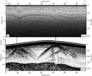
Fig. 2. Cross section from L1 to L10 showing (a) 900 MHz GPR profile with SCS and two depressions interpreted as snow bridges; and (b) the associated 40 MHz GPR profile with visible hyperbolas at 20–50m depth and associated reflection-free zones which we interpret as crevasses (C). SCS occurs on either side of the reflection-free zones and nearly reaches the bed.
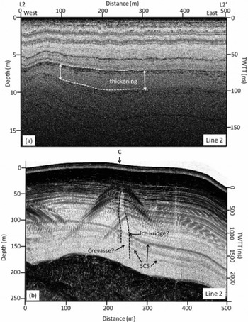
Fig. 3. Cross section from L2 to L20 showing (a) 900 MHz GPR profile with SCS thickening from west to east; and (b) the associated 40 MHz profile with visible hyperbolas at 20–50m depth and associated reflection-free zones which we interpret as crevasses (C). SCS surrounds the crevasse, and a potential ice bridge is located within the crevasse.

Fig. 4. (a) 900 MHz GPR profile collected from L3–L300 and parallel to the ice divide showing thickening SCS; (b) 40 MHz unmigrated profile collected from L3‘–L3’ showing strong bedrock reflection, SCS and cross-cutting horizons (CC); and (c) migrated 40 MHz GPR profile collected from L4–L40 showing corrected bed topography, cross-cutting horizons that have been partially removed but in an area that we interpret to contain avalanche debris resulting in no stratigraphy, and primarily SCS throughout the rest of the profile.
GPS and velocity
We conducted a standard, rapid static GPS survey at a 150 m grid spacing to determine surface ice-flow velocities. We used a Trimble 5700 control unit with a Zephyr Geodetic antenna as a continuously running base station between 31 May and 12 June 2011. We used a second Trimble 5700 with Zephyr Geodetic antenna to locate 29 stakes installed in a grid pattern covering the central region (750 m x 785 m) of the ice divide on 31 May. Each stake remained in place following the initial GPS measurement and was remeasured with GPS on 12 June. We used standard methods with Trimble Geomatics software to post-process the GPS data. The difference between corresponding point locations of each stake was used to calculate surface flow vectors (Fig. 1b; white arrows) to compare with our modeled velocity field (discussed below). The resulting displacements ranged from ∼35 to 540 mm. Position uncertainty estimates include a systematic ±5.0 mm error associated with the Trimble 5700 control unit, a 5.9 mm post-processing baseline error using the Canadian Spatial Reference System, and a ∼5.0mm error estimated from the field measurements based on the dimension of each velocity stake hole relative to the GPS antenna placement. Our positional error (1erp) of 8.4 mm accounts for the baseline and field measurement error assuming that the systematic error cancels. The uncertainty in velocity estimates (1eru) based on the 13 days of measurements and standardized to represent m a- 1 was 0.472 m a- 1 . The baseline distance was <0.5 km in all cases. We assume minimal melt and minimal associated seasonal variability in ice-flow velocities based on a cold snowpack (-18°C) and a likely frozen bed.
Field results
High-frequency (900MHz) radar profiles show mostly SCS and easily traceable isochrones across the entire plateau (Figs 2a, 3a and 4a). Stratigraphy appears to thicken in the northeast region of the ice divide relative to the rest of the glacier (Figs 3a and 4a, thickening). Low-frequency (40 MHz) radar profiles collected in south-north orientations parallel to the ice divide (Fig. 4b and c) reveal primarily SCS extending nearly to the bed (Fig. 4b and c). Ice depths range from 140 to 250 m, with shallower regions generally to the south and west of the divide and deeper regions to the east and north (Fig. 1). Maximum ice depths are located to the northeast of the ice divide immediately below exposed steep rock cliffs that bound the glacier (Fig. 1b, depth contours). This is the same location where a greater thickness between isochrones occurs in the 900 MHz radar data. Some crosscutting diffractions also appear near this region (Fig. 4b, CC) that can be partially removed via migration. However, following migration much of the stratigraphy in this region is removed. We interpret the cross-cuts and lack of stratification in the migrated profile (Fig. 4c) to represent intermixed debris deposited from occasional avalanche events occurring off the steep cliffs to the northeast.
We interpret a series of south-north-trending crevasses from the combined high- and low-frequency GPR profiles (Fig. 1b, interpreted crevasses). The 900MHz profiles collected from west to east across the divide reveal concave depressions in stratigraphy which we interpret to be sagging snow bridges over buried crevasses (Fig. 2a and c). Visual observations made from high vantage points in the field confirm these south-north-trending snow bridges. Low-frequency profiles suggest that in some areas these crevasses reach surprising depths (>150 m). Under higher gain settings (not shown), profiles collected across the ice divide reveal continuous stratigraphy visible on either side of a reflection-free zone that almost reaches the bed, suggesting that this crevasse may penetrate to bedrock (Figs 2b and 3b, crevasse). The reflection-less area and bounding stratigraphy is typical of GPR-imaged crevasses (e.g. Reference Arcone, Delaney, Noon, Stickley and LongstaffArcone and Delaney, 2000). Note that some faint reflections at 120160 m depth occur within the interpreted crevasses (Fig. 3b, ice bridge); we interpret these as frozen layers that bridge between crevasse walls, a common occurrence in large and deep crevasses. The crevasses are 5-14 m wide in GPR profiles and they narrow towards the north. However, the profiles were collected slightly oblique to the interpreted crevasse orientations, resulting in imaged crevasses likely appearing wider than they actually are. Radar and field observations show that the ice-divide crevasse is ∼500m long and extends from the satellite peak base to the ice-divide center. It does not appear to propagate to the base of the Main Peak of Mount Hunter. The flanking crevasses appear to propagate parallel to the ice divide and across the entire basin.
Velocity measurements reveal typical saddle flow on Mount Hunter, with surface velocities as low as 0.983 ±0.472 ma–1 at the center of the ice divide and as high as 15.0 ± 0.472 m a- 1 towards the calving ice cliffs (Fig. 1b). The divide is oriented north-south with primary flow directions in the center of and across the divide to the east and west. Ice flow from the North Peak and a satellite southern peak of Mount Hunter dominate the saddle flow dynamics, creating oblique flow directions at more distant regions from the divide center. Using an extension-positive and compression-negative sign convention, surface strain rates calculated from GPS-measured surface velocities (Fig. 5) range between 0.001 and -0.001 ±0.001 a- 1 ; the extensional values are on the low end of the required strain rates for crevasse initiation (Reference VaughanVaughan, 1993). We suggest that this ice is relatively strong due to low annual temperatures and a lack of debris or water within the domain, requiring higher surface strain rates for surface fractures to occur. The northern region of the divide is dominated by compressional ice flow from Mount Hunter which we argue counters the extensional divide flow, minimizing the possibility for crevasse formation in this area. In contrast, principal strain axes (Fig. 5) show maximum strain rates up to 0.002 ±0.001 a- 1 at the south-central ice divide where we see the crevasse buried at 50m depth and potentially reaching the bed. GPR profiles show this crevasse propagating and narrowing (Figs 2b and 3b, crevasse) south to north along the ice divide, eventually closing off as it reaches the aforementioned compressional zone (Fig. 5). Principal strain axes are also oriented perpendicular to crevasse orientations (Fig. 5) as expected (Reference Daellenbach and WelschDaellenbach and Welsch, 1993; Reference Harper, Humphrey and PfefferHarper and others, 1998). We use the calculated strain rates with caution because the uncertainty approaches strain-rate values due to the short time period over which the velocities were measured at this site. However, the general trend in observed velocities, resulting strain rates and crevasse patterns provides some confidence that our data are valid. There is potential for higher strain rates at the surface near the ice cliffs where surface exposed crevasses exist; however, velocities were not measured in these areas due to lack of safe access. We also do not assess the impact of multiple crevasses on strain-rate or stress patterns (e.g. Reference Sassolas, Pfeffer and AmadeiSassolas and others, 1996) which may be important here.

Fig. 5. Interpolated surface strain rate (contours) with extension-positive (blue) and compression-negative (red) sign convention and sigma-1 principal strain axes (extension arrows) calculated from measured surface velocities (black arrows), relative to the interpreted crevasses (double dashed lines).
Modeling Methods and Results
Modeling methods
We use a 3-D finite-element (COMSOL Multiphysics) numerical model to reproduce stress distributions that may lead to crevasse formation. Numerical model dimensions and boundary conditions were determined from field data collected in May 2010 and May–June 2011 (Fig. 6a, boundary conditions). All flow is the result of gravitational forcing. Ice flow from the divide axis is terminated at two icefalls. The longitudinal extent of the divide is terminated by the north and south peaks of Mount Hunter. The surface and icefall boundaries are treated as free surfaces with no applied stress. Other lateral boundaries are treated as zero-flux boundaries. Temperature data collected from a firn-core hole and from 4 m deep firn pits extracted in 2011 reveal polar conditions (–188C average temperature) and suggest the bed is likely frozen. This temperature estimate is in good agreement with an environmental lapse rate established by records from automatic weather stations at nearby Denali base camp (2380ma.s.l.) and higher on Mount McKinley (5750 ma.s.l.) (Reference Winski, Kreutz, Osterberg, Campbell and WakeWinski and others, 2012). We therefore assigned a no-slip basal boundary condition. We do not emplace variable temperature-dependent constraints on the model. The model geometry is defined by surfaces interpolated from GPS ice surface elevation measurements and ice depth data from migrated 40MHz GPR profiles. The model ice surface and bed cover the entire ice divide and are extrapolated using a least-squares polynomial regression from GPR cross sections and topographic US Geological Survey 1 : 24 000 elevation data (1998). The model is set up in two stages. The first model stage produces a material density gradient using a mesh with 551 355 tetragonal elements with an average element quality and node spacing of 0.717 and 7.58m, respectively, with a mesh resolution gradient that becomes finest (<1 m) within the density gradient and firn transition zone (Fig. 6b). The second stage is used to determine ice flow patterns and uses the density gradient as an initial condition. The second-stage grid is composed of 822 879 tetragonal elements distributed within the ice domain. An average mesh element quality and node spacing of 0.770 and 6.81 m was used, respectively with increased mesh resolution in zones expected to have large strain rates. We developed the depth-density profile (Fig. 6c, density) from a firn core collected at Kahiltna Pass Basin (3100 m a.s.l., 23.13 m depth) in 2008 (Reference CampbellCampbell and others, 2012a). Based on the firn core, density, p, increases with depth, z, in the model following

Fig. 6. Numerical model set-up showing (a) boundary conditions where the base (red) is frozen with no slip, blue boundaries allow lateral slip with no normal velocity components, and green boundaries (and the surface boundary, not shown) are zero-stress boundaries meant to replicate the ice surface and icefalls; (b) mesh used to produce model Navier–Stokes solutions; (c) density solution; and (d) dynamic viscosity.
Below 97 m depth, a constant ice density (917kgm–3) is assumed. We also assume that firn depth remains unperturbed in this case and that the initial density gradient remained constant for all simulations.
We solve for conservation of momentum and mass for incompressible non-Newtonian ice flow. We assume that the velocity measurements taken at the Hunter ice divide from 31 May to 12 June are representative of steady-state conditions. Therefore we do not consider the possibility of domain volume and shape changes with time. Accumulation and ice removal rates are assumed to balance, and the solution is for steady-state flow conditions, given these assumptions. Ice viscosity is defined by the power-law equation
where n is a unit-less strain exponent (Reference Cuffey and PatersonCuffey and Paterson, 2010), 7 is shear strain, and m is a power-law parameter built into the software and used to scale viscosity. Dynamic viscosity values ranged from 7.9 x 10¹³ Pa s at the base of the icefall to 1.0 x10¹⁴Pas in the divide interior (Fig. 6d, dynamic viscosity). Values for n and m were determined by iterative optimization (e.g. Figs 6c and 7a) in order to produce the dynamic viscosity range approaching 1.0 x10¹⁴Pas, an estimated viscosity of cold ice (e.g. Reference MarshallMarshall, 2005), and we used values of 0.333 and 6.5 x 10⁸kgs–nm–1 for n and m, respectively. This m value (Fig. 6b) is equivalent to the recommended A value of 1.2 x 10⁻²⁵s–1 Pa-3 for Glen’s flow law at -208C and n = 3.0 (Reference Cuffey and PatersonCuffey and Paterson, p. 75).
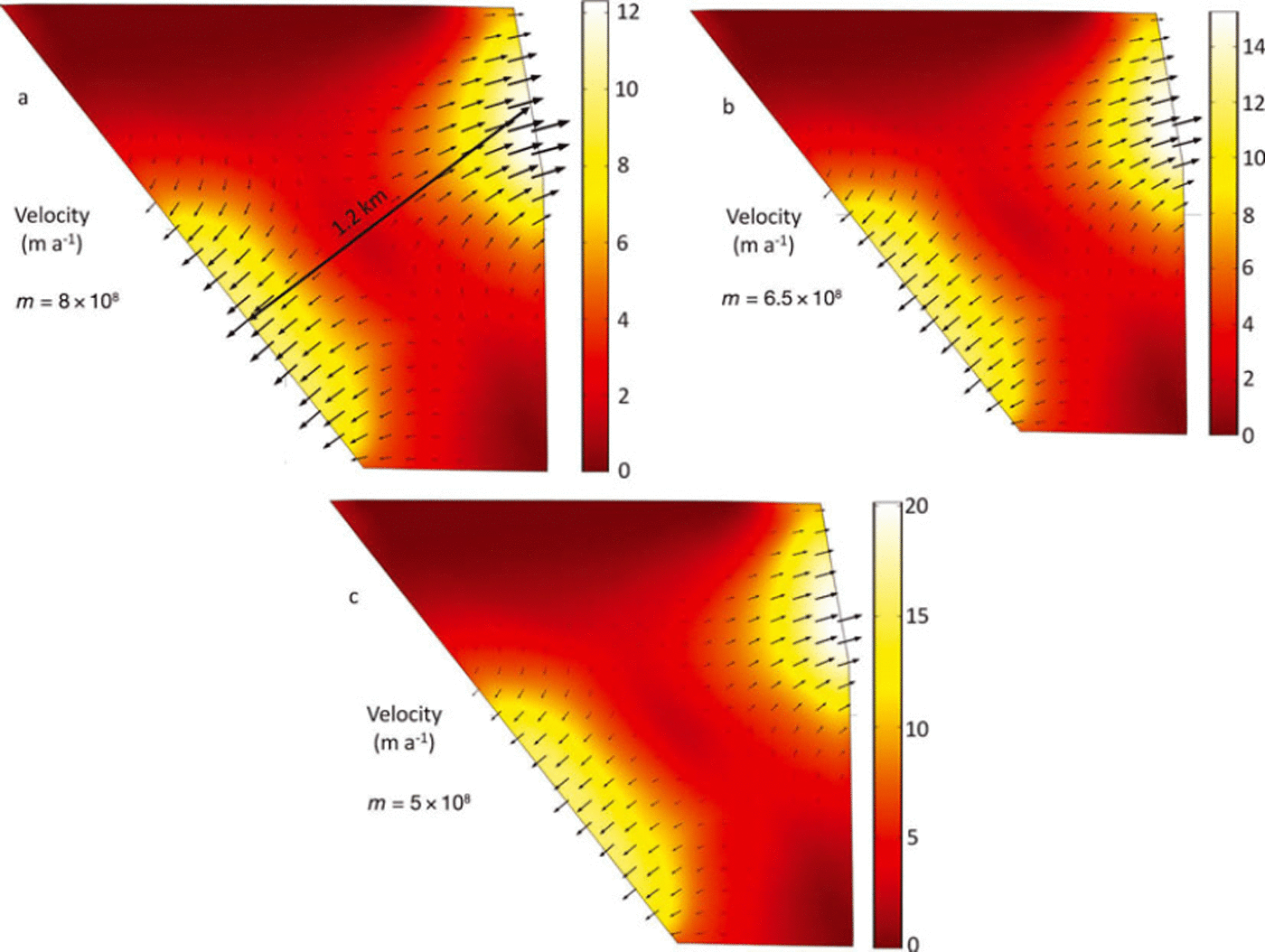
Fig. 7. Modeled velocities (m a–1) during the iterative optimization of the built-in power-law parameter (m) while trying to approach a dynamic viscosity of cold ice, 1014 Pas .
Model results
We follow the extension-positive/compression-negative sign convention. The gravity-driven ice flow produces a velocity gradient that increases toward the open vertical ice faces (Fig. 8a and b). Velocity magnitude ranges from 1.77 m a-1 along the ice divide to 15.3 ma-1 at the icefalls. North-to-south cross sections show a classic U-shaped valley velocity profile with a frozen no-slip bed (e.g. Fig. 8c). Horizontal normal strain rates (Fig. 8d) are greatest along the base of the cliffs where the no-slip basal condition intersects with the open stress boundary of the icefall. The maximum observed horizontal normal strain rate is 0.125 a-1, with most values ranging between 0.003 and 0.015 a-1. The resulting tensile stresses in these regions exceed 90 kPa, the required value to initiate crevassing (Reference VaughanVaughan, 1993; Fig 8e, red). The strain-rate profiles produced in this model indicate that crevassing would be most common ∼120 and ∼200 m upstream of both icefalls, and the crevasse would probably nucleate ∼50 and ∼40 m below the ice surface. The tensile stresses required to cause crevassing also appear close to the axis of the ice divide at the bed where bed slopes are steep (Fig. 8e, dashed circle).

Fig. 8. Model results showing (a) velocity for the solution with arrows denoting orientation, colors denoting magnitude, and white box representing the field survey region; (b) velocity cross sections normal to the axis of the ice divide; (c) cross section from a–a0 in (a) parallel to the ice-divide axis showing modeled velocities and field-measured velocities labeled above the black box for comparison; (d) horizontal coordinate normal strain rates; and (e) horizontal coordinate normal stresses, with stresses greater than 90 kPa highlighted in red, the black box representing the field survey region, dotted circle locating the high-stress location at the bed which seems to correspond with the ice-divide crevasse which reaches the bed, and the measured locations of surface exposed crevasses (EC) relative to the high-stress locations near the icefalls.
Field Data and Model Comparison
Field-measured and model surface velocities show reasonable agreement, which suggests some level of model robustness (e.g. Fig. 8c, a-a’). The in situ exposed crevasse locations (Figs 1b and 8e, EC) near the icefalls and outer extent of the GPR survey region closely match the high-stress locations estimated by the model. The high stress experienced at the icefall/bed interfaces seems to propagate inward toward the ice divide and reaches the surface in areas where we see surface or near-surface crevassing on the glacier (Figs 1b and 8e, EC). Likewise, the modeled southernmost region of the ice divide shows a high-stress zone at the bed where we also see the south-north-trending crevasse imaged with low-frequency GPR at depths beginning near 50m and potentially reaching the bed (Fig. 7e, dashed circle). This crevasse does not extend all the way across the ice divide, mirroring the decrease in stress (south to north) in the numerical models.
These crevasse geometries seem to suggest higher strain rates or rheologically weaker ice at depth, particularly in the south-central region of the divide and towards the icefalls. The GPR profiles show steeper bed terrain at the southern portion of the ice divide, where one crevasse is situated, and a relatively flat bed in the northern region of the divide
where no crevasses occur (Fig. 1b, ice depth contours). These results seem to confirm that the buried crevasses are significantly influenced by bed topography at this study site, which alters the stress pattern. The crevasse locations and orientations relative to principal stress axes and surface strain rates also provide supporting evidence for our topography-controlled interpretation. Also, although these results do not confirm crevasse formation at depth, they lean toward this interpretation. The modeled high-stress pattern at the ice/bed interface where the buried crevasse appears to reach in GPR profiles supports this interpretation. Likewise, the likelihood of 50 m of accumulation being deposited over a surface-formed crevasse without filling it is minimal, though not impossible.
Uncertainties and Assumptions
Uncertainties exist within field data and modeled results presented here, which must be thoroughly considered. First, the GPR data used to develop the bed topography covered only 0.5 km2 of the total ∼-1.5km2 study area, so extrapolation was required outside the survey grid. GPR profiles were migrated prior to developing the bed topography (e.g. Fig 4c); however, there is likely some error associated with the bed interpretation due to complex topography and manually picking bed depths. This error is likely smaller than the extrapolation error considering bed reflections were strong. The GPS data represent another source of uncertainty because both the time period between measurements (∼13 days) and the associated distances in which the glacier ice moved (∼3-53 cm) were small. Where measured velocities were lowest (∼1-2ma– 1 ) , displacement uncertainty approaches 50% of the total distance in which the velocity stakes moved. Conversely, the higher velocities are well above estimated uncertainties, so we have greater confidence in these measurements. Regardless, all calculated ice-flow vectors provide a realistic representation of velocities relative to the surrounding topography, which provides some confidence in the methods and measurements.
The timescale of the measured velocities is only 13 days, whereas the formation of stratigraphy and crevasses integrates years of accumulation and strain history; these time differences are not considered when interpreting the results. These model results are diagnostic force-balance calculations that produce a velocity field consistent with the ice geometry but do not reveal transient details or relationships between mass balance and dynamics. The model provides a relative comparison of stresses and strain rates spatially over the ice divide and we suggest that these variations in stresses and strain rates are heavily influenced by bed topography and icefall boundary conditions. Although the strain-rate values calculated from GPS surface velocities did fall within crevasse-forming rates accepted within the literature, we suggest caution with these results because of (1) the time discrepancies between crevasse formation and the field study, and (2) the large uncertainty associated with the calculated strain rates. We suggest future studies of similar ice-divide sites which incorporate mass balance, flow history and more extensive spatial and temporal controls on glacier and crevasse geometries to determine relationships between longer-term strain histories and the evolution of crevasses.
Conclusions
Our field results may provide the first GPR images recorded of buried crevasses reaching bedrock in a cold-based mountain glacier. Our data suggest that they formed at depth and that their locations and dimensions are likely controlled by complex bed topography. The icefalls located to the east and west of the ice divide produce significant tensile stress at the icefall/base interface which propagates obliquely from the bed into the firn towards the ice divide. The cold ice resists fracturing until within a few hundred meters of the ice divide where tensile stress exceeds tensile strength. A localized high-stress region buried at the model divide seems to correspond well with a buried crevasse imaged in GPR profiles collected over the real divide. Results from numerical models suggest that strain rates at the Mount Hunter ice divide approach 0.015 a- 1 , which falls within the range of strain rates (0.004-0.16a- 1 ) that have been known to generate crevasses, according to previous analytical studies.
Acknowledgements
We thank David Vaughan for helpful comments during the initial stages of the manuscript and Gordon Hamilton for assistance with GPS uncertainty analysis. Funding was provided by the American Alpine Club, Denali National Park Murie Science and Learning Center Fellowship, and the Dan and Betty Churchill Exploration Fund. We also thank the University of Maine, Dartmouth College, the US Army CRREL, Denali National Park and Preserve, Talkeetna Air Taxi, John Thompson and Dominic Winski for providing equipment and field support. Nate Lamie, Steven Decato and Jesse Stanley (CRREL) also provided significant technical support prior to and following field seasons.


