

1. Executive summary
Solvency II allows insurers to assess regulatory minimum (“Pillar 1”) capital requirements based on insurers’ own internal models of risks, subject to these models meeting regulatory standards. In addition to the measurement of individual risks, a key element of these models is the level of diversification assumed between risks. This can reduce the amount of capital required by up to 70%Footnote 1 compared to the sum of individual risk capital requirements before diversification.
There is a need to justify such diversification benefits given the size of these, both in terms of empirical data (where available) and also with regard to underlying economic and other inter-dependencies between risks. This paper focuses on identifying the variables driving dependencies between risks to help justify diversification benefits, and is split into two parts.
The first part of this paper considers dependencies between different market and credit risks. There is generally sufficient empirical data to assess the degree to which different markets are correlated under normal conditions, but such correlations may overstate the degree of diversification in stressed conditions where there is less data available. There is a need to overlay empirical correlations with expert judgement to allow for how risks may interact at the tail which drives capital requirements.
Based on analysis of historical market crashes; academic, industry and other papers; and forward-looking scenarios, the paper identifies three components to stressed markets:
-
• fragilities which build up in the financial system such as excessive credit growth, or financial de-regulation;
-
• initial shocks to the system such as rate rises or economic downturns which can expose these fragilities; and
-
• transmission of shocks between markets, for example due to reduced investor appetite and/or forced sales coupled with monetary and fiscal responses.
From this we can identify linkages between market and credit risks in stressed market conditions to help adjust correlation assumptions for tail dependency.
The second part of the paper considers wider dependencies with other risk categories such as insurance risk (including lapse and expense risk) and operational risk. There is usually little data to assess correlations with these risks, which also vary from company to company, so there is a greater degree of reliance on expert judgement and consideration of drivers of dependency. Key drivers identified include:
-
• economic downturns which may affect lapses and other risks;
-
• pandemics and other extreme scenarios which can impact financial markets; and
-
• reputation damage which can lead to lower sales, higher lapses and higher unit costs.
This paper is intended to provide a basis for insurers to identify dependencies between risks to meet regulatory requirements, and to ensure correlation assumptions driving diversification benefits are sound.
2. Introduction
As part of the Statistical Quality Standards which insurers’ internal models must meet under Solvency II, Delegated Regulation Article 234 (Diversification Effects) specifies:
“The system used for measuring diversification effects referred to in Article 121(5) of Directive 2009/138/EC shall only be considered adequate where all of the following conditions are met:
-
(a) the system used for measuring diversification effects identifies the key variables driving dependencies;
-
(b) the system used for measuring diversification effects takes into account all of the following:
-
i. any non-linear dependence and any lack of diversification under extreme scenarios;
-
ii. any restrictions of diversification which arise from the existence of a ring-fenced fund or matching adjustment portfolio;
-
iii. the characteristics of the risk measure used in the internal model;
-
-
(c) the assumptions underlying the system used for measuring diversification effects are justified on an empirical basis.”
This paper seeks to identify key variables driving dependencies as per delegated Article 234 (a) above, and also to highlight any lack of diversification in extreme scenarios as per (b) (i). The paper does not seek to measure diversification effects on an empirical basis, though empirical data is investigated as it is a prima facie indicator of dependency between risks.
The paper focuses on Market, Credit, Insurance and Operational Risks which contribute to Solvency II capital requirements. It does not consider Liquidity Risk nor Strategy Risk in detail.
Dependencies are generally modelled using either copula or variance-covariance matrix approaches, both of which are based on correlation assumptions between different risk pairs. Note that while dependency is used interchangeably with correlation throughout this paper, there are differencesFootnote 2 . The paper does not aim to cover different measures of correlation nor aggregation methods in detail. Instead, the author would refer the reader to Dorey et al. (Reference Dorey, Joubert and Vencatasawmy2005) and Shaw et al. (Reference Shaw, Smith and Spivak2010) which provide good coverage of these topics.
Correlation estimates used to investigate dependencies are generally based on the Pearson correlation measure, and are classed as low for correlations <30%; medium for correlations ≥ 30% and <60%; and high for correlations ≥60%. To understand the impact of different correlation assumptions, Appendix I illustrates the impact of sample correlation assumptions.
While the author’s experience predominantly relates to UK life insurance, it is hoped that this paper will be of wider interest to those modelling diversification benefits for Solvency IIFootnote 3 and economic capital modelling purposes.
2.1. Limitations of the paper
The topic of dependencies between risks is wide ranging and difficult to cover completely. The author would draw the reader’s attention to the following limitations of this paper:
-
• The focus of the paper is on dependencies over a 1-year period consistent with the timeframe of Solvency II, but considering longer timeframes may give a different perspective of dependencies: for instance, climate change may have little impact on mortality rates and assumptions over a 1-year period, nor on bond defaults and downgrades, but considering say a 20-year period, climate change could have a significant impact both on mortality rates and on default rates for certain bond sectors such as oil and gas.
-
• The paper’s focus is on the drivers of dependency rather than the calculation of empirical correlation estimates, which are just used as indicators of dependency. For simplicity, empirical estimates of correlations are generally based on the Pearson linear correlation measure but there are a number of limitations to this measure compared to other measures such as the Spearman rank measure of correlation – see Embrechts et al. (Reference Embrechts, McNeil and Straumann1999) for a more detailed discussion of correlation measures.
-
• The author was unable to analyse data for private equity and private credit and therefore was unable to draw on conclusions on dependencies between these asset classes and other markets and risks.
Part I Market and credit risk dependencies
3. Empirical analysis
Empirical correlations can be estimated from market data in liquid markets and these are a starting point for correlation assumptions between most market and credit risks. However, a key contention of this paper is that while empirical correlations can point to dependencies between risks, they are flawed, and need to be supplemented with wider analysis.
For the purposes of this paper, empirical correlations have been estimated from:
-
• MSCI local currency equity price indicesFootnote 4 ;
-
• Government bond yields from the Bank of EnglandFootnote 5 and US Federal ReserveFootnote 6 ;
-
• Currency rates from the Bank of EnglandFootnote 7 ;
-
• Commodity prices in US Dollars from the US Federal ReserveFootnote 8 ;
-
• Credit spreads: ICE Bank of America Merrill Lynch (BofAML) US Corporate indexFootnote 9 ;
-
• CBOE VIX index of equity option volatilityFootnote 10 ;
-
• Inflation and GDP statistics from OECDFootnote 11 ;
-
• US Commercial Property data sourced from the US Federal ReserveFootnote 12 ; and the
-
• Wilshire US Real Estate Investment Trust (REIT) Total Market IndexFootnote 13 .
However, there are issues with empirical correlation estimates for property risk: these are discussed in section 3.4.4 below.
Comparison is also made with global default data from Moody’s 2021 annual corporate bond default surveyFootnote 14 , but data is limited – see section 3.4.5.
Note that many other sources of data are available, and these may yield different correlation estimates.
3.1. Correlations between different risk types
Chart 1a below highlights the links between rolling (overlapping) 12-month changes in bond spreads, equities and point-in-time option implied volatilities based on data from 1997 (from when spread data is available from ICE) to end 2020.

Chart 1a. Key market variables and events – Equities, Bond Spreads and Volatility.
From this chart we can see that there is a significant positive correlation between falling equity markets and rising bond spreads (or negative correlation between rising equity markets and rising spreads), particularly in stressed markets such as those during the Global Financial Crisis of 2007/09. A similar relationship can also be seen between equity market movements and implied volatility levels. As we shall see, in stressed conditions, risk aversion can lead to a re-pricing of risks with adverse consequences for equity and corporate bond values, as well as higher option prices and implied volatilities.
Considering equity market correlations with safer assets, for the purposes of this paper, US Treasury Bonds (“T-bonds”) are considered to be risk-free assets with nominal yields on US T-bonds a proxy for interest ratesFootnote 15 . From Chart 1b below, we may discern a correlation between falling equity markets and falls in US T-bond yields. In part this reflects risk aversion in stressed markets which will lead to investors switching into highly rated government bonds and other low risk assets, driving down yields on these. Also, central banks tend to react to falling markets by lowering interest rates and, since 2009, by using Quantitative Easing (QE) to print money which is then used to buy assets and support markets, driving down bond yields in the process.
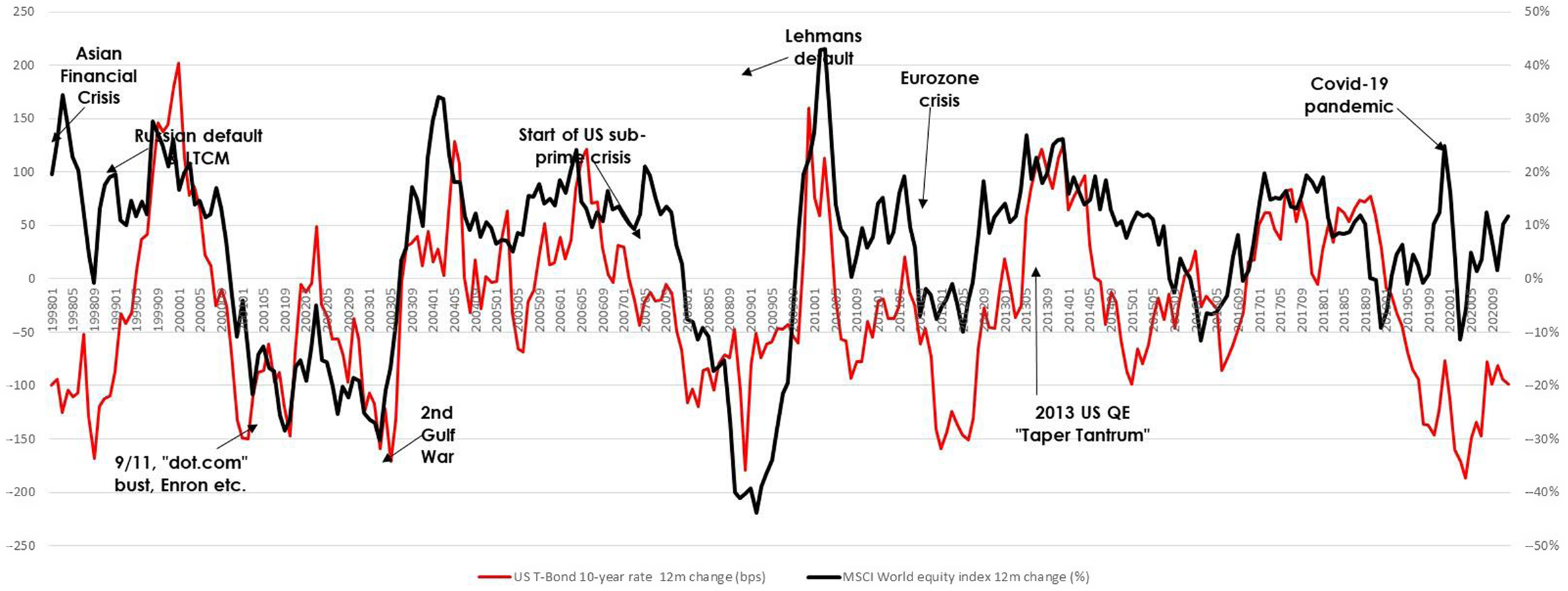
Chart 1b. Key market variables and events – Equities and T-bond yields.
These relationships are reflected in empirical correlation estimates which suggest medium/high correlations between most market variables as the following Table 1 shows.
Table 1. Estimated Correlations between Market Variables from 1997 to 2020

Note that the positive correlation between equity market falls and US T-bond yields decreases with bond termFootnote 18 . This may be because in the past the US Federal Reserve has cut short-term base rates as a response to market crashes. However, this relationship may no longer be valid as base rates have been cut close to zero and there is limited potential for base rates to go negative, while QE has increasingly been used to support markets and this will drive down yields at longer terms.
Looking only at changes since 2009, correlations between the MSCI World equity index and 2-, 10- and 30-year US T-bond rates are 20%, 59% and 59% respectively, highlighting the sensitivity to the time period used. The low short-term correlation may be due to low, stable base rates since 2009, with the US target federal funds rate unchanged between 2008 and 2015 at 0.25% and never exceeding 2.5% p.a. sinceFootnote 19 . Meanwhile the impact of QE can be observed most recently in early 2020, when sharp market falls due to COVID-19 triggered unprecedented central bank intervention, with the combination of QE and “flight to quality” pushing US 10-year T-bond rates from 1.92% p.a.at the start of the year to 0.66% p.a. by mid-year.
As well as the time period over which they are assessed, correlations between equities and T-bond rates are also sensitive to the measure of change. The figures above are based on absolute changes in rates, defined as:
 $${\rm{Change}} = \left\{ {{\rm{T - bond}}\,{\rm{rate}}@\,{\rm{t}}} \right\}-\left\{ {{\rm{T - bond}}\,{\rm{rate}}@{\rm{t - }}12\,{\rm{months}}} \right\}$$
If instead we based correlations on relative changes in rates defined as:
Change @ time t = [{T-bond rate @ t}/{T-bond rate @ t-12 months}] – 1we get revised correlations between the MSCI World equity index and 2-, 10- and 30-year US T-bond rates of 49%, 46% and 37% which are noticeably lower, highlighting the sensitivity of empirical correlation estimates to different measures such as absolute or relative changes.
3.1.1. Correlations between currencies and other market risks
A key market risk not considered above is currency risk. Here correlations with other market risks can be less clear cut as they may depend on the exchange rate in question. By way of example consider the following Table 2 of correlations for rolling 12-month movements in the Sterling values of the US Dollar, Japanese Yen and the Australian Dollar with other market variables from October 1993 (12 months after “Black Wednesday” and Sterling’s exit from the European Exchange Rate Mechanism (ERM) to float freely on markets) to 2020:
Table 2. Estimated Correlations between FX Rates and Other Market Variables from 1997

From these correlation estimates, we can observe the following:
First, correlations between different exchange rates differ – for instance there is a high correlation between changes in the Sterling value of the US Dollar and Japanese Yen, but a low correlation of the former with changes in the Sterling value of the Australian Dollar.
Second, there would appear to be at least a low/medium negative correlation between rising equity markets and rising Sterling values of the US Dollar and Yen assets (or a low/medium positive correlation of US Dollar and Yen exchange rates rising against the pound and falling equities). This could be because in stressed market conditions, investors tend to buy US Dollars and Yen as part of a “flight to safety” to safer assets and currencies.
By contrast, the correlation between the Sterling value of the Australian Dollar is slightly positive with equity markets.
The following Charts 2a and 2b compare changes in the Sterling value of US and Australian Dollars with UK equity movements.
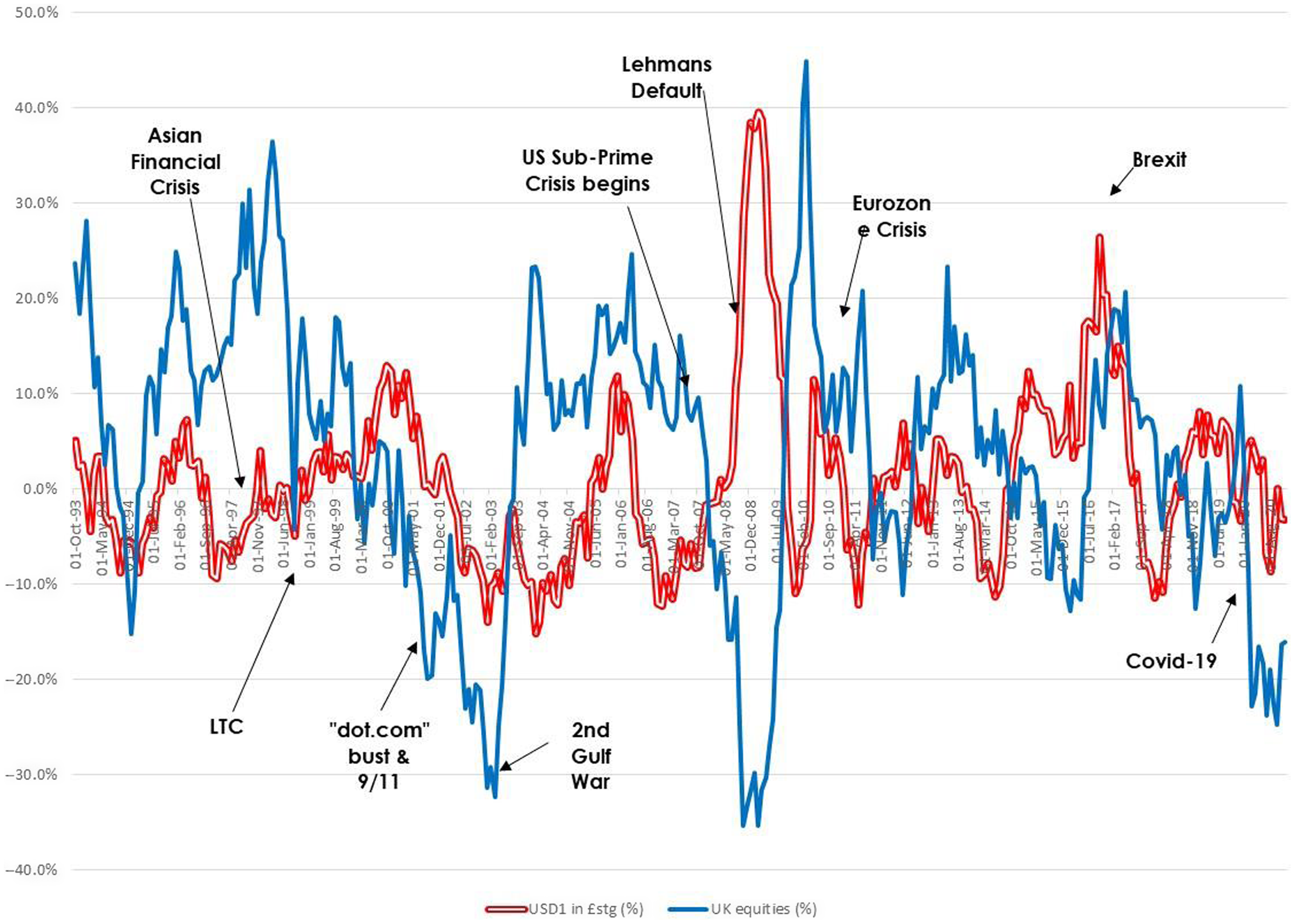
Chart 2a. Sterling: USD exchange rates and UK equities from 1992.

Chart 2b. Sterling: AUD exchange rates and UK equities from 1992.
Of note is the sharp rise in the value of the US Dollar against the Pound during the Global Financial Crisis arising in conjunction with a sharp fall in UK equities. This may point to a higher degree of dependence at the tail between UK equity market falls and Sterling deprecation against the US Dollar than might be suggested by the empirical correlation estimate.
This correlation between sterling depreciation and falling equity markets is not observed when considering the value of the Australian Dollar against the Pound. If anything, the Australian Dollar has often depreciated when UK markets are falling. One reason for this may be the “carry trade” where investors borrow money in Yen and other currencies with low interest rates to invest in currencies with higher interest rate – such as the Australian Dollar during the mid-2000s. This is a risky strategy as it leaves investors exposed to falls in the higher interest rate currencies, and is sensitive to investor appetite. In stressed conditions where investors become more risk averse, they will seek to unwind positions in the higher interest rate currencies, which may explain the depreciation of the Australian Dollar during the Global Financial Crisis. However, looking forward, this relationship between the Australian Dollar and the carry trade may no longer hold, highlighting the perils of trying to infer future correlations from the past.
Finally, considering exchange rates and bond yields, there is a negative low/medium correlation between rising UK Gilt yields and rises in US Dollar and Yen against Sterling. Examining possible drivers for this correlation:
-
• This correlation could be because of higher UK interest rates and yields boosting the value of Sterling.
-
• Alternatively, it could be because better UK economic prospects are driving up both bond yields and Sterling – correlation does not imply causation, and often there may be other underlying variables (in this case UK GDP growth) driving the correlation.
-
• As we shall see, the Bank of England’s 2019 stress test for banks involved a “run” on Sterling pushing up UK bond yields, i.e. implying a strong positive correlation between rising UK bond yields and rises in US Dollar and Yen against Sterling, highlighting how empirical estimates may not capture tail risks such as a loss of investor confidence in the UK.
Again, the correlation between UK bond yields and changes in the Sterling value of the Australian Dollar exhibits a different pattern.
The above highlights that there is no “one size fits all” correlation assumption when it comes to currency dependencies. Depending on exposures to different currencies, there may be a need to either set correlations by currency, or to group exposures to currencies with similar characteristics (like the US Dollar and Yen above).
3.1.2. Correlations between commodities and other market risks
Another market risk where correlations vary by sub-type is commodity risk. Within commodities, we can distinguish between different types of commodity such as copper, oil and gold. While the first two are commodities required by the real economy, the third is more a store of value and is seen as a “safe haven” in turbulent markets.
As a result, correlations with equities and bond yields will vary by type, as can be seen from the following Table 3 of correlations estimated from 12-month changes from January 1991:
Table 3. Estimated Correlations between Commodities RatesFootnote 20 and Other Market Variables

All other things being equal, higher oil prices increase production costs and dampen demand, but they will be a boon for oil and gas stocks, so the impact of oil prices will vary by equity market depending on the weighting of the market to oil and gas stocks. Moreover, higher oil and copper prices may also be indicative of broader economic growth which may also help drive up share prices, illustrating the multi-faceted nature of dependencies between commodities and shares, and between market risks more widely.
The link between economic growth and prices of commodities like oil and copper may also be a reason for the medium positive correlations observed between these and bond yields.
By contrast, gold’s status as a safe asset in turbulent times leads to low negative correlations between gold and both equities and bond yields with gold prices often rising in stressed markets when equities are falling along with bond yields. This relationship is not clear cut however and there are other factors which affect the gold price such as production and consumer demand.
Finally, the correlations above are based on US Dollar prices of commodities as commodity prices are typically quoted in US Dollars. Correlation estimates will change if looking at say the Pound Sterling equivalent of commodity prices, though these estimates would implicitly capture an element of currency risk as well.
3.1.3. Correlations between inflation and other market risks
Another key market risk variable is inflation. In assessing correlations between inflation and other market risks, there is a need to distinguish between:
-
• Actual inflation relating to changes in retail prices over the past month/year; and
-
• Implied inflation which is inferred between from the difference between nominal and index-linked bonds, and which is a measure of market expectations of future inflation.
Implied inflation will vary by term, and will be relevant to the market consistent valuation of future inflation-linked liabilities and expenses, as well as values of general insurance claims where there is an inflationary element to claim payouts. For economic capital purposes, we will be looking to model changes in implied inflation rates. However, for the purposes of modelling expense and claim outflow over the coming year, actual inflation would be more relevant.
The following Chart 3 compares UK actual and implied inflation from 1986Footnote 21 :

Chart 3. UK Actual v Implied Inflation.
We can see there is a significant disconnect between actual inflation at a given point in time, being the change in prices over the past 12-months, and implied inflation at that point in time inferred from nominal and real Gilt yields, highlighting the need to consider these separately when analysing dependencies.
As an example of this disconnect, we can discern a shift in actual inflation following Sterling’s exit from the European Exchange Rate Mechanism (ERM) in September 1992, after which the Bank of England adopted an inflation targeting approach to monetary policyFootnote 22 . This has proved successful in taming inflation which has generally remained below 5% p.a., with the Retail Price Index (RPI) measure averaging 2.7% p.a. since October 1992, consistent with the Bank of England’s target of 2.5% p.a. for RPI. However, market expectations of inflation took some time longer to adjust, and only started to align with the Bank of England’s target after the Bank of England was made independent in 1997.
Since 1997, market implied UK inflation has generally been around 3% p.a. This is higher than the Bank of England’s target rate, which could reflect the risk the Bank of England might abandon this for a looser target, but it may also have to do with demand from pension scheme and others for index-linked Gilts to hedge inflation-linked liabilities. This will reduce index-linked Gilt yields relative to nominal Gilt yields and push up implied inflation, highlighting another difference between actual and implied inflation.
Examining correlations between UK actual and implied inflation rates with rolling 12-month changes in 10-year Gilt yields and global equities in Table 4 below, we can see significant differences in correlations depending on which measure we consider:
Table 4. Estimated Correlations between Inflation Rates and Other Market Variables from 1986

From above, we can see that actual changes in prices in the past 12-months have a high correlation with current implied inflation, which we may expect, but will have little relevance to changes in implied inflation which will impact on economic capital.
Changes in UK implied inflation are highly correlated with changes in UK nominal Gilt yields, which is what we might expect given the link between inflation and bond yields, while there is a low correlation between global equity movements and changes in UK implied inflation (correlations between UK equities and UK implied inflation will be covered in section 3.4.1 below).
3.2. Correlations between government bond yields
As well as dependencies between different types of market risk (equity, interest rate etc.), we also need to consider dependencies within market risk types, including interest rates in different countries and currencies. Table 5 below considers correlations between rolling 12-month absolute changes in US, UK, German and Japanese 10-year government bond yields from 1990.
Table 5. Correlations between 10-Year Bond Yield Changes from 1990

There is broadly a high correlation between bond yields of these highly rated sovereign issuers. The lower correlations for Japanese bond could in part be because Japanese bond yields were significantly lower over the period, with yields less than 2% p.a. since 2000. Just looking at changes over the 1990s, the correlations between Japanese bond yields and US, UK and German yields are significantly higher at 62%, 75% and 83% respectively.
The high correlations may be expected as interest rates in one currency will be influenced by interest rates available in other currencies. US bond yields in particular have a strong bearing on other yields. This was illustrated by the spike in US bond yields in 1994 following unexpected tightening of US monetary policy. This led to US 10-year bond yields rising 201bps from 5.83% p.a. at the start of the year to 7.84% p.a.at year end. This helped drive similar rises elsewhere with 10-year UK Gilts yields rising by 234bps from 6.25% to 8.59% p.a., 10-year German Bunds rising 163bps from 5.83% to 7.46% p.a. and 10-year Japanese government bonds rising 116bps from 3.40% to 4.56% p.a. over the year.
Another example of the impact of US monetary policy on wider bond yields was the “taper tantrum” that followed the announcement of the US Federal Reserve in May 2013 that it was going to scale back bond purchases under its QE programme. US 10-year T-bond yields rose sharply from 1.7% in April to 3.0% p.a. by year end. Over the same period and UK and German 10-year bond yields rose by 137bps and 60bps respectively, though Japanese 10-year bond yields only rose by 10bps.
Note for lesser rated sovereigns such as Greece, it may be better to assess government bonds yield dependencies based on the yields on highly rated sovereign bonds (e.g. German Bunds) plus a sovereign spread. The latter is likely to widen in stress conditions.
Also, bond markets where there are currency restrictions (e.g. Malaysia) may be substantially uncorrelated with other bond markets as these restrictions will lead to a disconnect between local and global rates.
3.3. Correlations between equity markets
Examining correlations between rolling 12-month changes in MSCI price indices from December 1987 (December 1992 for China)Footnote 23 in Table 6a below:
Table 6a. Correlations between Changes in MSCI Price Indices from 1987

As we might expect there is generally high degree of correlation between developed equity markets, except perhaps for Japan. Asian and emerging markets also exhibit a high degree of correlation which is to be expected as China and other Asian markets form a large part of the MSCI Emerging Market index.
There appears to be lower levels of correlation between western and Asian/emerging markets but this is due to the Asian Financial Crisis of 1997/98 where Asian shares saw significant falls while western markets were growing. If we just look at rolling 12-month returns based on data from January 1999 (first 12-month period to January 2000) in Table 6b below, correlations between western and Asian/emerging markets are ca.20% higher:
Table 6b. Correlations between Changes in MSCI Price Indices from 1999

It is worth noting recent increases in China’s weight in global equity indices. In 2019, MSCI quadrupled the weight given to Chinese A shares in its ACWI global (developed + emerging markets) index, so that Chinese equities now account for over 5% of that indexFootnote 25 . Not only will this increase global equity portfolio allocations to Chinese equities, it will also increase the degree of correlations between global indices and Chinese shares.
Other observations:
-
• The high degree of correlation between the MSCI World index and US equities is to be expected given that the US accounts for ca. 2/3rds of that indexFootnote 26 .
-
• Smaller markets may be dominated by individual firms or sectors which may have a bearing on correlation. For example, the insurer AIA currently accounts for over 27% of MSCI’s Hong Kong equity indexFootnote 27 while financial services accounts for 47% of that index.
-
• Linked to this, different correlations may exist between broad and narrow indices of the same market. For example, looking at the broader MSCI UK All Cap index which is available from November 2007, the correlation of rolling 12-month returns with the MSCI World index is slightly higher than the correlation between the standard MSCI UK index, with its narrower market coverage, and the World index (86% v 84%)Footnote 28 .
3.4. Limitations of empirical analysis
There are a number of notable limitations in using empirical analysis to identify dependencies:
Nature of dependencies
-
1. Empirical correlations provide an indication of the direction and strength of dependencies between risks, but they don’t really provide an explanation for why the dependency exists in the first place.
-
2. Being based on historical data, they implicitly assume that historic dependencies between risks continue, but there may have been changes in the interaction between risks which mean historic relationships are no longer relevant. Empirical analysis needs to be supplemented with a forward-looking view of dependencies.
-
3. Depending on the time period used, there is the possibility that empirical estimates straddle periods where the relationships between risks was different, with the resulting correlation not a satisfactory measure of either period – see 3.4.1 below.
-
4. Empirical correlations may not fully capture tail dependence for risks which are not closely correlated in normal market conditions but which may be heavily correlated in stressed conditions – they may implicitly average out correlations resulting in an estimate that doesn’t reflect either state of the markets.
-
5. Some empirical correlations may be spurious, driven by random coincidence rather than any true dependency between risks.
-
6. Correlations do not necessarily imply causation – it may be that two risks are not directly linked but both may be affected by another variable.
Data issues
-
7. Empirical estimates are based on the shortest dataset, for example correlations involving credit spreads may only be based on data back to 1997 where spread data is based on that available from ICE which is only available from that date.
-
8. Results may be sensitive to the frequency of data, the length of the dataset and the correlation measure used – see section 3.4.2 below.
-
9. There will be a degree of statistical error around empirical correlations depending on the length of datasets – see section 3.4.2.1 below.
-
10. Following on from 4.above, where risks are more heavily correlated in stress conditions, empirical correlations may drift downwards over time as data is added when conditions are benign, but can then spike up again in stress conditions.
-
11. Risks may be correlated but with a time lag, in which case there will be a need to identify the extent of the lag and correct correlation estimates where appropriate – see for example the links between equity market and GDP falls in section 3.4.3.
-
12. Correlation estimates may be distorted by implicit smoothing in data, for example in valuation-based property indices – see section 3.4.4.
Consistency
-
13. Unadjusted empirical correlations may be inconsistent with each other, resulting in correlation matrices which do not meet Positive Semi Definite (PSD) criteria of consistency which underpins copulas and other aggregation methodsFootnote 29 .
3.4.1. Changes in dependency over time
An example of changing relationships between risks, and the distortion they can create with empirical estimates, is the correlation between UK equities and Gilt yields changes. If we look at rolling 12-month changes in Gilt yields and the MSCI UK equity index, we get very different answers depending on how far back we go, as illustrated by the following Table 7:
Table 7. Correlations Between Changes in UK Equity Prices and Gilt Yields

We can see that there has been a marked change in the correlation between UK equities and Gilt yields, from a negative correlation between falls in equities and Gilt yields (positive correlation between Gilt yield rises and equity falls) in data going back to 1970, to a positive correlation between falls in both equities and yields.
Looking at rolling 5- and 10-year correlations between 10-year Gilt yields and equities in Chart 4a below, the shift appears to occur in the early 2000s.

Chart 4a. Rolling correlations between changes in UK equities and 10-year Gilt yields.
An explanation for the change would be the shift from the high-inflation, high interest rate environment that existed from the 1970s to the early 1990s to a lower inflation and rate paradigm. Prior to Sterling’s exit from the ERM in September 1992, there were frequent spikes in inflation, either due to oil price and other shocks or due to an overheating economy. These drove up Gilt yields and base rates, which in turn led to economic downturns and equity market falls, hence the correlation between yield rises and equity falls.
As noted in section 3.1.2, following the ERM exit, the Bank of England adopted an inflation targeting approach to monetary policy which proved successful in taming inflation and “boom and bust” economic cycles. Now, rather than rate rises triggering equity market falls, interest rates and Gilt yields may be more driven by equity market falls, with the Bank of England responding to market crises such as the Global Financial Crisis of 2007/09 and more recently market falls due to COVID-19 by cutting rates and buying bonds under QE. This would explain why the current direction of correlation relates to falls in both Gilt yields and equities.
It is interesting to note that correlations between changes in UK equities and implied inflation in Chart 4b below show a similar pattern:
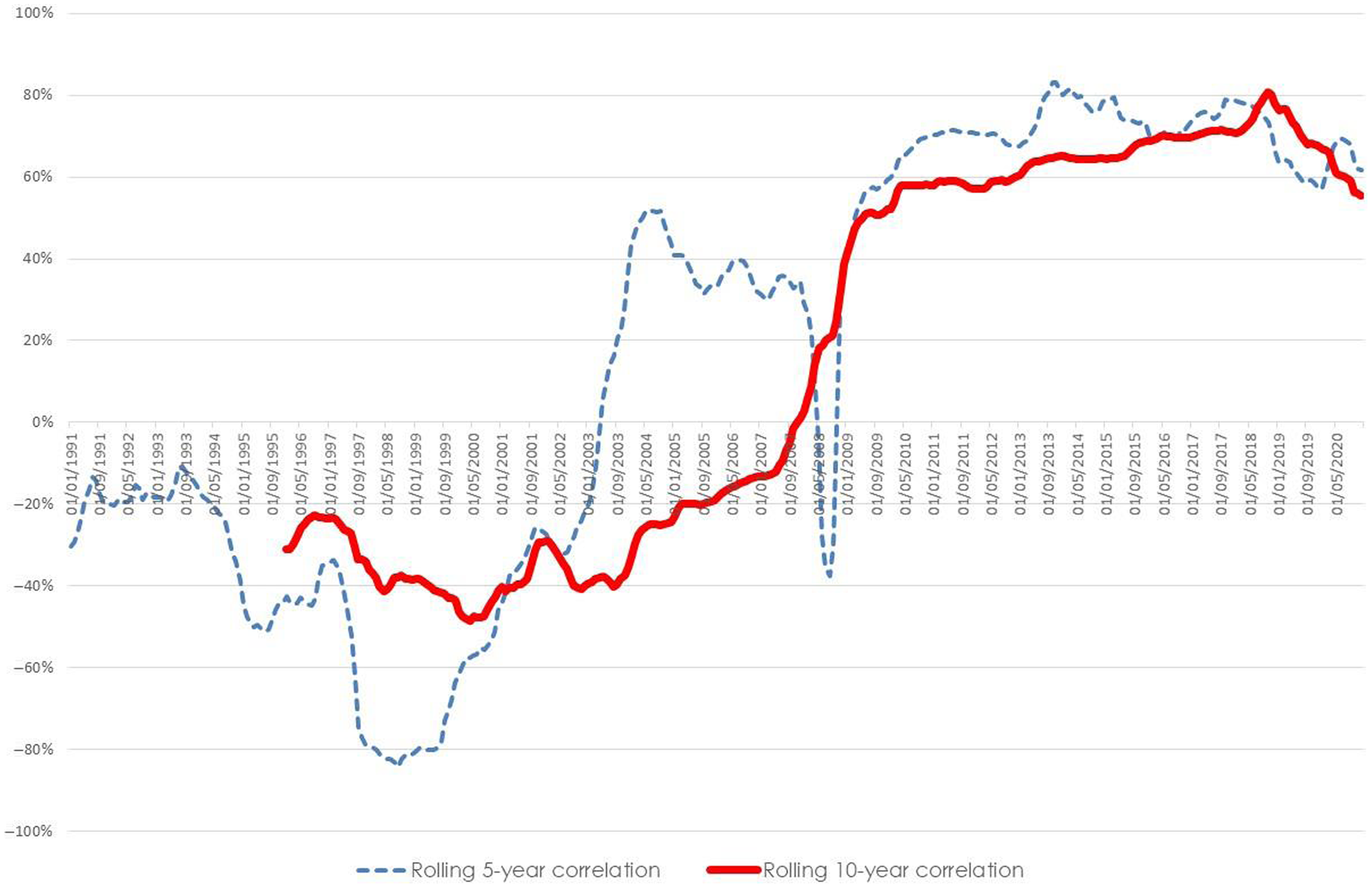
Chart 4b. Rolling correlations between changes in UK equities and 10-year implied inflation.
Again, until the early 2000s, rises in implied inflation were negatively correlated with equity market rises (/positively correlated with equity falls) as higher inflation – and higher market expectations of inflation, as reflected in implied inflation – would have fed through into higher base rates which will have had a negative impact on equities.
More recently, that direction has changed so that now equity falls are correlated with reductions in implied inflation. It may be that QE in response to more recent equity market falls has driven down implied inflation as well as nominal Gilt yields and/or that market falls have led to lower expectations for economic growth and inflation.
These examples highlight the need for care in choosing the timeframe over which we base empirical correlation estimates. Consideration needs to be given to paradigm shifts such as the shift a low inflation environment in the 1990s, and whether data before is relevant. In the case of UK equities and Gilt yields, while we have data going back to 1970, using this data leads to correlation estimates which do not reflect the current correlation between Gilt yields and equity markets, so it would be probably more appropriate to base correlations on data from the 1990s or later.
However, as we shall see, the dynamic that previously existed between rising rates and Gilt yields driving down equity markets has not disappeared altogether, and there may be a case for carrying out sensitivity testing to the impact of a future change in the direction of UK equity and Gilt yield correlations.
3.4.2. Sensitivity of estimates
Empirical correlation estimates are not just sensitive to the time period over which they are assessed, they are also sensitive to the choice of risk variable. From section 3.1, we saw how correlations between rolling 12-month changes in equities and bond yields varied depending on whether we were looking at absolute or relative changes in yields.
Another example would be the correlation between the MSCI World index of equities and VIX. The correlation in Table 1 of −58% was based on the correlation between the 12-month change in the equity index with the point-in-time value of VIX. If instead we looked at the correlation of rolling 12-month changes in the equity index with (a) rolling 12-month absolute changes in VIX; and (b) rolling 12-month relative changes in VIX, we would get revised correlation estimates of −56% and −49% respectively.
Yet another example would be where we looked at monthly changes as opposed to rolling 12-month changes. From Table 1, the correlation between rolling 12-month changes in MSCI World equities and absolute changes in US 10-year T-bond yields is +54%, but if we looked at monthly changes, the correlation estimate would be significantly weaker at just +33%.
In practice, we would base correlation estimates on measures corresponding to individual calibrations of risk. For instance, if our model of corporate bond spreads was based on rolling 12-month absolute changes in spreads, then this is the measure we would use in estimating correlations, but it would be useful to consider the sensitivity of correlation estimates to different measures.
Finally, the above correlations relate to the Pearson measure of correlation. If instead we used the Spearman measure of rank correlationFootnote 30 between rolling 12-month changes in MSCI World equities and US corporate bonds spreads, we would get a revised correlation estimate of −48% as opposed to −58% based on the Pearson measure.
Further details on the sensitivity of correlation estimates can be found in section 7.5 of Shaw et al. (Reference Shaw, Smith and Spivak2010).
3.4.2.1. Parameter estimation error
As well as the sensitivity to different data and measures, there will also be a degree of statistical parameter estimation error in empirical estimates, which can sometime be substantial. Taking the example of equity returns and corporate bond spreads, from Table 1, we arrived at an empirical correlation estimate of −58% based on 276 overlapping 12-month periods from 1997 to 2020. Using the Fisher transformationFootnote 31 to assess the degree of statistical error around this estimate gives a range of −49% to −65%, and this would be larger for smaller datasets, which illustrates how significant parameter estimation error can be.
3.4.3. Lag effects
An example of lag effects we may need to allow for in correlation estimates is that between equity returns and GDP growth. If we take the example of US quarterly GDP growth rates and equity returns from 1970, the unadjusted empirical correlation is only +4%, and only +7% based on data from 2000. This seems counter-intuitive as we would expect a link between stock markets and economic growth.
However, markets often react in anticipation of events so they may rise or fall before rises and falls in GDP come through in economic statistics, while market crashes such as those during the Global Financial Crisis can in themselves trigger a wider recession. For these reasons, we may expect a lag between markets and GDP changes. If we allow for a one quarter lag between equities and GDP, the revised correlation estimate based on data from 1970 is +31%, and +44% based on data from 2000.
Lag effects can also be observed between equities and unemployment rates, as the following Chart 5 of US equities and unemployment rates illustrates.

Chart 5. Quarterly US equity returns and unemployment rates from 2000.
Of particular note is the unemployment rate during the Global Financial Crisis. This peaked at 9.9% in Q4, 2009 by which time equities (and bonds) were recovering from their trough in Q1 2009.
Similar effects can be seen during the “dot.com” bust of 2000/03 where peak unemployment was reached in Q2/Q3 2003 when markets were recovering strongly, and during the COVID-19 pandemic, where there was a sharp fall in markets in Q1 2020 but unemployment rose sharply in Q2 despite central bank intervention leading to a sharp recovery in markets. The lag between markets and unemployment rates may be expected as it may take time for economic downturns to translate into job losses.
Lag effects are significant in the context of a one-year value at risk (VaR) assessment such as that required under Solvency II. While over the 2–3 years of a market downturn like that of the Global Financial Crisis we may see significant declines in both equities and GDP say, over the 12-month period where we might see the worst equity market falls, only part of the fall in GDP may come through due to a lag effect. It may be appropriate to scale back correlations between the one-year impact of GDP falls with one-year equity returns and other market variables to reflect this partial impact.
3.4.4. Property risk
The empirical analysis above does not include property risk but index data is available such as MSCI’s Investment Property Databank (IPD) indices for commercial property, and residential property indices like the Nationwide House Price Index for UK housing.
However, caution should be exercised in using commercial property index data to assess correlations. These indices are usually based on subjective property valuations (though transaction-based indices may also be available in some cases). A problem with valuation-based indices is that there can be implicit smoothing in the index in part because of valuations being anchored on historic transactions. This results in the volatility of commercial property being understated and could also distort empirical correlation estimates with other risks.
Implicit smoothing is covered in the Investment Property Forum’s 2007 paper on index smoothingFootnote 32 and also Booth and Mercato (Reference Booth and Mercato2003). These also set out approaches to “de-smooth” indices, correcting for historic bias in valuations. Empirical property correlations should be calculated based on de-smoothed as well as unadjusted indices in order to gauge the impact of smoothing on correlation estimates.
Booth and Mercato (Reference Booth and Mercato2003) also highlights differences in performance assessed against different indices, and different indices could also give rise to different empirical correlation estimates. Where data for different indices exists, the sensitivity of empirical correlations to different data sources should be assessed.
As an alternative to valuation-based indices, correlations could be calculated based on indices of Real Estate Investment Trusts (REITs) where available. These should reflect market views on the value of property assets and may be a timelier reflection of changes in value than valuation-based indices. However, a problem with basing property correlations on REITs is that being listed on stock exchanges, REITs will be affected by wider rises and falls in other shares and so will be more correlated with equity markets than direct investment in property.
To illustrate the difficulties of assessing property correlations empirically, consider the following example of US commercial property price correlations with US equities. Sourcing commercial property price data from the US Federal Reserve and looking at quarterly changes from Q1 1978 against quarterly returns on the MSCI US equity price index, the standard deviation of unadjusted property price changes is 2.9%, and the correlation of this unadjusted data series with US equities is slightly negative at −7.5%.
There is a significant degree of correlation (ca.40%) between returns in successive quarters suggesting smoothing in data. De-smoothing the data in line with the adjustment outlined in section 3.6 of Booth and Mercato (Reference Booth and Mercato2003), the standard deviation of quarterly changes is substantially higher at 4.4% but in this instance the correlation with US equities is only slightly larger at −11%.
Considering next the alternative of using REIT indices, data for the Wilshire US Real Estate Investment Trust Total Market Index goes back to Q1 1978. The standard deviation of quarterly changes in this index is higher again at 5.3% but crucially, the correlation between this index and the MSCI US equity price index is +60%, i.e. a high positive correlation compared to the slightly negative correlation assessed based on the US Federal Reserve’s commercial property data. Comparing quarterly changes graphically from 2000 in Chart 6 below:

Chart 6. US equity, REIT and commercial property quarterly returns from 2000.
We can perhaps see a degree of correlation between US REIT and broader US equity indices, particularly during the Global Financial Crisis. The sharper fall in the REIT index in Q4 2008 may be due to concerns over commercial property valuations following the default of Lehman’s, which had a significant property portfolio to be realised.
Notwithstanding the low negative empirical correlation estimates above, we also see a sharp fall in the unadjusted (smoothed) commercial property index in this period, albeit with a lag with the index reaching its trough in Q1 2010 when equities had recovered strongly from their trough in Q1 2009. We could adjust the calculation of empirical correlations between property and equity returns allowing for say a 2-quarter lag, which would change the correlation from −7.5% to +14%, but even this revised figure doesn’t reflect the sharp falls in both US equity and commercial property indices during the Global Financial Crisis.
This example highlights the difficulties of basing property risk correlations using empirical data. The high correlation between equities and REITs could be due to REITs being stock market vehicles as much as any links between equity and property markets, but the low correlation between the US Federal Reserve commercial property data and US equities does not properly capture tail events seen in historic data. Significant expert judgement is required to arrive at a suitable correlation figure.
Complicating matters is the lag between changes in equities and property values. This could be a function of implicit smoothing in property valuations but it could also reflect underlying delays in the transmission of market shocks to property markets: market falls could in time lead to a “credit crunch” affecting the roll over commercial property loans, triggering distressed sales. As noted in section 3.4.3 above, this lag is significant in the context of a one-year value at risk (VaR) as while over the 2–3 years of a market downturn we may see significant falls in both property and equity markets, over the 12-month period where we might see the worst equity market falls, only part of the fall in property values may come through due to a lag effect. It may be appropriate to scale back correlations between one-year property returns with equities and other market variables to reflect this partial impact.
3.4.5. Bond default and downgrade risk
From section 3.1, there is strong correlation between corporate bond spread indices with equities and other markets, but these index changes mostly relate to general movements in spreads as opposed to defaults and downgrades. Spread changes will be driven as much by changes in investor sentiment regarding credit risk as actual defaults and downgrades.
Spread changes will also be affected by bond market liquidity issues, with forced sales in stressed markets pushing down mark-to-market prices and pushing up spreads. In some instances, liquidity issues could cause spreads to exceed even pessimistic forecasts of defaults: in the aftermath of Lehman’s for instance, US investment grade corporate bond spreads exceeded 6% p.a. By contrast, the worst single year of the Moody’s 2021 Corporate Bond Default Survey was 1938 when the investment grade default rate reached 1.55%Footnote 33 .
Given the impact of investor perceptions of credit risk as well as market liquidity factors on spreads, there is a need to consider bond default and downgrades separately from spreads in assessing correlations.
Chart 7 below compares Moody’s yearly data on global investment grade and aggregate bond defaults with the investment grade US corporate bond spread index from 1997 (see section 3.1) as a proxy for global bond spreads.

Chart 7. Moody’s bond defaults and US IG corporate bond spreads 1997-2020.
In terms of correlations, the key issue to note is the limited data on investment grade defaults which are zero in most years, while others just relate to a single default – for example, the 2019 investment grade default figure is due to the bankruptcy of the Pacific Gas and Electric Company following forest fires in California for which it was held partially culpableFootnote 34 . This is likely to distort any empirical correlation estimate.
This could be addressed by incorporating downgrade losses, which are likely to be more important for investment grade bond portfolios anyway. Moody’s supply details of downgrade (and upgrade) rates as part of their annual default study, and losses on downgrade could be estimated by reference to historic differentials in corporate bonds yields for different ratings and terms, though this would not be a trivial exercise.
Notwithstanding the issues with limited data, from Chart 7, we can draw two broad conclusions. First, as we may expect, there is a link between bond defaults and bond spreads, particularly in stressed market conditions like the Global Financial Crisis. This isn’t perfect however, as spread rises may be driven as much by investor fears (e.g. of systemic risk issues during the Eurozone crisis) and liquidity issues as credit risk.
The other thing to note is the lag between spread rises, with their concurrent market falls, and defaults emerging. Taking the Global Financial Crisis as an example, spread started rising in H2, 2007 due to a mixture of credit concerns and a squeeze in liquidity caused by the US sub-prime crisis. The big surge in defaults however arose in 2008, and continued into 2009, even though bond spreads had started to recover after Q1, 2009.
This lag between market expectations of default, as expressed in spreads, and defaults themselves is to be expected, particularly as bonds usually go through a number of downgrades before finally defaulting. There may also be a lag in terms of how market downturns and financial crises transmit to the wider economy through a “credit crunch” triggering recession and defaults by non-financial issuers. As for property risk, there may be a case to scale back bond default and downgrade correlations with spreads, equities and other market variables for a one-year VaR assessment to allow for lag effects so that only part of any stress to defaults and downgrades comes through in the worst 12-month period for spreads etc.
3.4.6. Other counterparty default and downgrade risk
In terms of other counterparty defaults and downgrades, such as reinsurers and derivative counterparties, it will generally be impractical to assess these on an empirical basis due to the more limited number of counterparties involved. Instead, correlations are likely to be based on expert judgement.
3.4.7. Addressing limitations in empirical analysis
Given the limitations of empirical analysis, there is a need to supplement this with qualitative analysis to form a better understanding of dependencies. This should encompass analysis of
-
• historic periods of stress to better understand tail dependence;
-
• academic research and other papers on dependencies between risks, how these have changed in the past, and how these may change in the future; and
-
• forward-looking scenarios, again to understand how risks could interact in the future.
These are considered in the following sections.
4. Analysis of stressed financial conditions
Appendix II includes details of historic stress periods and how these affected multiple risks. Based on an analysis of these, the following observations can be made on the relationships between markets at the tail.
4.1. Equities and corporate bond spreads in stressed market conditions
There is a strong degree of correlation between equity falls and corporate bond spread rises in stressed conditions, though the link is not perfect. If we consider the peak 12-months movement in the ICE BofAML US Corporate Bond (C0A0) spread index from 1997, this was a rise of +456bps in the year to 31st October 2008, compared with the 99.5th percentile of the empirical distribution of rolling 12-month changes from 1997 of +428bpsFootnote 35 . The MSCI US equities index fell −37.5% in the same period, which would be close to the 98th percentile fall in the empirical distribution of US equities from 1997Footnote 36 . The peak fall in US equities since 1997 was −44.5% in the 12-months to February 2009 when the 12-month change in (C0A0) spreads was +296bps which would equate to the 98th percentile of the empirical distribution of spread changes.
The 98th percentile movement in equities/spreads when spreads rises/equity falls peaked suggest very high correlation but not 100% – otherwise both would have peaked at the same time. The close correlation can be explained by investor risk aversion affecting both corporate bond and equity markets in light of losses on US sub-prime securities and the subsequent default of Lehman’s in September 2008.
If we look at the “dot.com” bust, there were fewer extreme movements in both spreads and equities. The maximum fall in US equities over 2000/03 was −28% in the 12-months to end September 2001, which is unsurprising given the events of 9/11. This equates to a 97th percentile fall from the empirical distribution of US equity price changes from 1997Footnote 37 . However, there was only a + 32bps rise in spreads in this month, and spreads were only up +19bps on the year before, which equates to the 66th percentile of one-year movements from 1997.
The peak rise in spreads in the period 2000/03 was +86bps in the 12-months to end 2000, which would equate to the 92nd percentile of the empirical distribution of spreads. Over the same period, US equities fell by −14% which would equate to the 88th percentile of the empirical distribution of returns while the MSCI World index fell by −11%, which would be roughly the 84th percentile.
Another notable spread shock was the rise of +77bps in the 12-months to end July 2002, shortly after the WorldCom bankruptcy, one of the largest in US history. This equates to the 90th percentile of empirical spread movements. US equities fell by −7% in this month and were down −25.5% over 12-months which would be around a 96th percentile fall from the empirical distribution of price changes. From Appendix I, given a 95th percentile movement in risk A, the average movement in risk B is the 90th percentile assuming a + 75% correlation and a Gaussian copulaFootnote 38 , so we could infer a correlation of around +75% from the combination of spread and equity changes in the 12-months to end July 2002.
In general, the period of the “dot.com” bust again illustrates the close correlation of equities and spreads in stress conditions, but also that the correlation is less than perfect. This reflects different drivers – for instance, equity market falls were driven in part by a bust in internet stocks which were not major issuers of corporate bonds.
Finally, considering the recent COVID-19 pandemic, the initial shock led to a spike in spreads and sharp equity falls in February/March 2020 before intervention by the US Federal Reserve and other central banks on 23rd March stemmed market falls. At this stage, US corporate bonds had peaked at 401bps, up +276bps on the year before. This would be close to the 98th empirical percentile of spread changes. US equities fell −20.3% in the 12 months to 23rd March, broadly akin to the 92nd empirical percentile fall. Again, this points to a high but not perfect correlation between bonds spread and equity changes in stress conditions.
4.1.1. Bond default and downgrades in stressed market conditions
From section 3.4.5, Chart 7, we can see a clear link between bond defaults and downgrades and spread rises – and from above equity falls – in stress conditions such as the “dot.com” bust of 2000/03 and the Global Financial Crisis of 2007/09. Falls in the value of property and other collateral will exacerbate losses on default.
However, the correlation is not perfect. For instance, from the Moody’s 2021 default study, there was over US$2bn of investment grade defaults in 2005 in what was a positive year for equities, with the MSCI World index of developed market equities up nearly +14% on the year. Looking back further, there were no investment grade defaults in 1987 or 1988, despite the large equity market falls in October 1987.
Following on from section 3.4.5, there is also a lag between market falls and defaults coming through. This is illustrated by the continued rise in defaults caused by the COVID-19 pandemic over 2020 while markets recovered from their trough in March 2020: of US$228m of (mostly sub-investment grade) bonds and loans defaulting in 2020, 92% have arisen after Q1, at a time when bond spreads have fallen back to end 2019 levels and equity markets have risen on average by +60% since 23rd March 2020.
4.1.2. Derivative counterparty default and downgrades in stressed market conditions
Considering first derivative counterparties, the example of the Lehman’s default during the Global Financial Crisis highlights both how stressed markets could trigger counterparty default and how such a default could amplify a crisis. Amongst other things, market falls reduced the value of collateral held, while rising option prices post-Lehman’s increased the price of replacement hedges, exacerbating losses on default.
Looking forward, the move towards central clearing of derivatives should limit the impact of individual counterparty default, but it will not remove this entirely: even if central clearing can mitigate counterparty losses, the removal of an investment bank counterparty will limit market capacity to provide hedging solutions and will drive up the price of option protection and implied volatility.
Central clearing also creates a tail risk in respect of the failure of the central clearing house. While remote, this is not improbable: a notable feature of the 1987 stock market crash was the failure of the Hong Kong Futures Exchange clearing house, which required a government bailout, highlighting that even clearing houses could fail in extreme market eventsFootnote 39 . Were a major clearing house to fail, the impact on markets could be even greater than that of Lehman’s.
4.1.3. Reinsurance counterparty default and downgrades in stressed market conditions
Reinsurers are a key counterparty for most insurers. A notable failure during the Global Financial Crisis was AIG which amongst other things was a major reinsurance counterparty, as well as a key writer of bond default protection for other insurers. AIG was bailed out by the US Government due to the potential impacts of a default on other market participants, but this “near miss” highlighted the potential for market stresses to undermine reinsurance counterparties – and also that the Global Financial Crisis could have been so much worse.
Other victims of the crisis were monoline insurers such as Ambac and MBIA. These were AAA-rated insurers who obtained a premium from issuers to cover investor losses should the issuer default. This guarantee allowed issuers to share in the insurers’ AAA-rating, but heavy losses from US sub-prime and related bonds they insured led to Ambac declaring bankruptcy in 2010 while MBIA was downgraded to B in the same year. The failure of these guarantors led to mass downgrades of the bonds they guaranteed, further contributing to downgrade losses in the crisis.
Aside from AIG and the monoline insurers, other reinsurers suffered losses as a result of the crisis which resulted in many being downgraded. Among these was Swiss Re which was downgraded in 2008 due to market and credit losses which gave rise to a loss of CHF864mFootnote 40 . Looking forward, such reinsurer downgrades may give rise to losses due to the need to increase counterparty adjustments to reinsurance assets in the calculation of insurers’ technical provisions, highlighting the link between stressed markets and reinsurer counterparty losses.
Note that as well as market losses impacting on reinsurer financial strength and credit rating, catastrophic events can lead to large insured losses and drive down markets. An example of this would be 9/11. This gave rise to one of the largest cumulative insured losses of all time at US$26bnFootnote 41 . Of 20 major reinsurers, 14 were downgraded in the following two yearsFootnote 42 . Meanwhile MSCI US and World indices fell by −7.7% and −9.0% respectively in September 2001, and by −23% and −22% respectively over the following 12-months, while US investment grade corporate bond spreads rose by +52bps over the year.
That said, the costliest event for insurers to date was Hurricane Katrina in August 2005, with total losses of US$82bn. While this triggered reinsurer downgrades, the impact on markets was more muted: MSCI US and World equity indices only fell by −1.1% and −0.1% respectively that month with little impact on corporate bond spreads.
On balance, while reinsurers do seem to be vulnerable to the risk of downgrade in stressed market conditions, and while catastrophic events can also trigger market falls as well as large insured losses, the link is far from perfect. There may be no more than a medium correlation between reinsured default and downgrade and market falls.
4.1.4. Retail loan defaults in stressed market conditions
From section 3.4.3, falling markets are correlated with lower economic growth and higher unemployment, albeit with a lag. If we look at the Global Financial Crisis, market falls led to a “credit crunch” which transmitted market falls to the wider economy leading to recession and higher unemployment. In the UK for example, there was a peak-to-trough fall in GDP of ca. −6% while unemployment rose from 5.35% in Q2, 2007 to 8.0% by Q1, 2010.
The economic downturn and higher unemployment led to a marked increase in mortgages in arrears with UK mortgage arrears rising from just over 40,000 at the end of Q2, 2007 to a peak of nearly 81,500 in Q1 2009Footnote 43 . They then decreased as banks took possession of homes and sold these off. Exacerbating losses, UK house prices declined by nearly −20% in the same period, though they recovered from Q1, 2009Footnote 44 .
Note that even before the crisis, unsecured loan losses were rising in the UK with the number of personal insolvencies in the UK spiking upwards by 60% in 2006 to 100,000Footnote 45 . It is likely that high house prices were masking underlying issues with mortgage creditworthiness that were then exposed by the fall in house prices during the crash. In this way falls in house prices during a crash can crystallise credit losses on mortgages, which may in turn lead to losses on bonds linked to these.
The link between market downturns and mortgage and other loan defaults is far from perfect however. During the 2000/03 stock market downturn, while US unemployment rose, UK unemployment declined and UK house prices grew strongly during the period.
More recently, although the COVID-19 pandemic led to sharp market falls initially as well as a modest increase in UK unemployment from 4% to 5.8%, arrears totals have stayed broadly similar over 2020 at just under 40,000, while UK house prices have risen +7% over 2020.
4.2. Property in stressed market conditions
From section 3.4.4, there were sharp fall in US commercial property markets during the Global Financial Crisis. UK and other commercial property markets also experiencing sharp falls at this time, while there were also sharp falls in house prices, with US house prices falling −17.5% between June 2007 and March 2009Footnote 46 and UK house prices falling −20%. This suggests at least a medium correlation between property, equities and bond spreads.
However, one would argue against a high correlation for two reasons. First, as noted in section 3.4.4., there is a lag effect which should temper correlation assumptions. The US property index only reached its trough 12 months after the low point for US equities in Q1 2009. The UK reached its trough sooner in Q2 2009, but again this was at a time when UK equities were recovering strongly. Average US house prices, which were already falling before the crisis began, continued falling as markets recovered from March 2009, not reaching their trough until early 2012, by which stage they had fallen a further −8%.
Second, it is also worth noting that during the “dot.com” bust, property prices were generally growing while equity prices were falling, so the connection between property and equity markets is not as strongly linked as say equity and corporate bonds.
4.3. Interest rates in stressed market conditions
Mindful of the potential knock-on impact of market falls on the wider economy, central banks have frequently responded by easing monetary policy. For instance, during the “dot.com” bust, having initially increased federal funds rates from 5.5% to 6.5% p.a. over 2000, the US Federal Reserve then cut base rates to 1.75% p.a. by end 2001, 1.25% by early 2002 and 1.00% by June 2003. Similarly, having increased base rates to 6% p.a. in 2000, the Bank of England then cut these to 3.5% by July 2003.
The rate cuts helped drive down bond yields with 10-year US T-bond yields decreasing from 6.45% p.a.at the end of 1999 to 3.37% by May 2003, though the reduction in 30-year yields was smaller, falling from 6.48% p.a.at the end of 1999 to 4.59% by May 2003. The fall in UK Gilt yields was more muted, with 10-year yields falling from 5.38% p.a. at the end of 1999 to 4.16% by May 2003 while the 25-year yield was generally higher over the period than 4.23% at end 1999.
During the Global Financial Crisis, central banks responded to falling markets not just by cutting short-term base rates but also by buying bonds under QE programmes. In doing so, monetary policy started to directly impact on longer-term bond yields.
The US federal funds rate was cut from 5.25% p.a.to 4.25% by end 2007, to 2% by April 2008 and then to 0.25% by the end of 2008Footnote 47 , with the US Federal Reserve also starting to buy US$600bn in mortgage-backed securities from November 2008 as part of QEFootnote 48 . Similarly, the Bank of England cut base rates from 5.75% p.a. in July 2007 to 2% by end 2008 and 0.5% from March 2009Footnote 49 , at which stage it started buying £165bn of Gilts as part of QE. The European Central Bank (ECB) cut its deposit facility rate from 3% p.a.in mid-2007 to 2% at end 2008 and 0.25% in April 2009Footnote 50 , with a €60bn QE programme buying covered bonds starting in May 2009.
Combined with investor risk aversion and flight to quality, this monetary stimulus pushed down government bond yields. 10-year US T-bond yields fell from 5.03% p.a.at the end of June 2007 (when troubles were starting to emerge with US sub-prime assets) to 4.04% at end of 2007 (−99bps over H2 2007), then to 3.83% by the end of August (pre-Lehman’s) and 2.25% by end 2008, a fall of −179bps over the year, before recovering to 3.53% by mid-2009.
UK 10-year Gilt yields did not fall as far, but still fell from 5.36% p.a.at the end of June 2007 to 4.52% p.a. (−84bps) at the end of 2007 and 3.39% by end 2008 (−113bps over the year). They then spiked upward by nearly +70-bps in January 2009 as there were concerns over the solvency of the UK government following the bailout of banks. The price of insuring UK government bonds over 5 years rose from less than 20bps in August 2008 to more than 100bps by the end of the year and to ca.150bps by mid-January 2009Footnote 51 . However, the introduction of QE in March 2009 helped drive 10-year Gilt yields down to 3.30% at end March, before yields recovered to 4.20% p.a.by the end of 2009.
German 10-year Bund yields also saw significant falls, from 4.56% at mid-2007 to 4.21% by end 2007 (–35bps) and 3.05% by end 2008 (a fall of −116bps over the year). Ominously, however, the yields on 10-year Greek government bonds rose from 4.53% p.a. at end-2007 to 5.08% at end-2008, as the 10-year spread over Bunds rose from +32bps to +203bps. This rise in sovereign spreads would ultimately lead to the Eurozone crisis of 2010/12.
From the Global Financial Crisis, we can see a link between equities and spreads on the one hand and interest rates and highly rated government bond yields on the other. Central banks respond to market turmoil by cutting rates and pushing down longer-term bond yields using QE. Yields on US T-bonds and other highly rated government bonds will also be driven down by a flight to quality into safer issues, but for lesser rated sovereign issuers, the same investor risk aversion could see government bond yields rise due to a rise in sovereign spreads.
This dynamic was also seen more recently with the response to the COVID-19 pandemic. The US Federal Reserve cut its federal funds rate by −150bps in March 2020 to near zero. While other central banks had less scope to cut rates, the Bank of England also cut its base rate from 0.75% p.a. to 0.1% p.a.at this time.
Central banks also expanded QE programmes. The Federal Reserve announced US$700bn of asset purchases, and crucially expanded the range of bonds it would buy to include some sub-investment grade bonds which stemmed a rout in markets for these. The Bank of England bought another £200bn of Gilts while the ECB launched a €750bn programme to drive yields down.
Coupled with a flight to quality, this result was a sharp fall in government bond yields with 10-year US, UK and German bond yields falling by −122bps, −46bps and −24bps in Q1 2020 to 0.7%, 0.36% and −0.54% p.a. respectively. However, investor risk aversion saw yields on 10-year Greek bonds rise from 1.42% to 1.97% p.a. over Q1 and 2.05% by the end of April, before falling back to 1.32% at the end of Q2 as markets recovered.
4.3.1. Upward shocks to interest rates
It is important to note that the experience of the Global Financial Crisis and COVID-19 may not always hold for future market crises. There is another dynamic between interest rates and markets where interest rates may be the cause of market falls as opposed to just being driven down by these. An upward shock to rates, particularly if unexpected, can trigger falls in equities and other markets.
An example of this is the sharp rise is US T-bond yields in 1994 (see section 3.2). In the first instance, US stocks fell initially but recovered, in part because the rate rise came to be seen as indicative of the health of the US economy. However, UK, European and Asian (ex Japan) shares ended down −9.9%, −8.4% and −20.5% respectively due to the impact of higher rates.
This link is far from perfect, and even unexpected monetary tightening may not trigger wider market falls. For instance, the “taper tantrum” of 2013 – where mooted reductions in QE by the US Federal Reserve triggered a spike in global bond yields – did not stop the MSCI World index rising +26.3% over the year, with little impact on corporate bond spreads. However, the MSCI Emerging Markets index fell −5.0% over the year, so these markets are likely to be more vulnerable to tighter US monetary policy.
Another dynamic to consider is the impact of inflationary shocks on both interest rates and equity markets. A classic case of this is the 1973/74 oil shock, which led to the MSCI World index falling by −39.2% in the 12 months to end September 1974 while long-term US T-bond yields rose by +88bps in the same period. While central banks have been successful in keeping inflation low in recent times, there is still a risk of a shock to inflation either because of a geopolitical event like the Yom Kippur War in 1973, or at an individual country level, because of a sharp depreciation in currency. This could lead to higher base rates to combat inflation which would push up bond yields and also depress economic demand, which could in turn lead to equity falls and rising bond spreads.
4.3.2. Real yields and implied inflation rates in stressed conditions
Rises in inflation can trigger interest rate and wider market stresses, but market stresses will also have a bearing on real yields and market implied inflation rates. The following Chart 8 highlights UK and USFootnote 52 real yields and implied inflation rates, highlighting periods of market stress.

Chart 8. Change in US and UK real yields and implied inflation rates from 2000.
Looking first at real yields, like nominal yields, QE and a “flight to quality” could drive these down in stress conditions, as happened with the COVID-19 pandemic.
However, the experience of the Global Financial Crisis suggests other factors at play: while generally US and UK real yields were falling from the start of the crisis in June 2007 to August 2008, they spiked upwards after Lehman’s: 10-year US real yields rose + 174bps from 1.78% p.a. at the end of August to 3.52% by the end of October 2008 before falling back, while 10-year UK real yields rose + 181bps from 0.97% p.a. at the end of August to 2.78% by the end of November 2008. Real yields at other terms also rose in this period – from August to October 2008, US 5- and 20-year yields rose by +235bps and +106bps, while from August to November 2008, UK 5- and 20-year real yields rose by +292bps and +83bps respectively.
The spike in real yields after Lehman’s is puzzling as nominal yields were falling in the same period. Index linked government bond markets are smaller and less liquid than nominal markets, and these could have been more affected by forced sales, for example to raise cash to meet margin calls.
In any case, rising real and falling nominal yields resulted in a significant reduction in implied inflation. In the UK,10-year implied inflation fell from 3.56% p.a. at the end of August to 1.23% by the end of November 2008, before rising to 2.23% p.a. by March 2009 and 3.31% by end 2009. Similarly, US 10-year implied inflation fell from 2.33% p.a.at the end of August to 0.39% by the end of November 2008, before rising to 1.45% p.a. by March 2009 and 2.58% by end 2009. This highlights the potential shifts in implied inflation rates in stressed conditions which could have significant implications for valuations based on these.
Examining other periods of stress, the fall in US real yields and more limited reductions in UK real yields during the 2000/03 downturn are broadly consistent with changes in nominal yields in the same period, while the rise in real yields during the 2013 US QE “taper tantrum” is again broadly consistent with rises in nominal yields.
In summary, in stressed conditions, drivers of nominal yield changes are likely to have a similar impact on real yields, but other factors could lead to a disconnect like that in the months after Lehman’s, so the correlation between the two will be far from perfect. Different changes in real and nominal yields could lead to significant variations in implied inflation at the tail.
4.4. Currencies in stressed market conditions
The evidence of the Global Financial Crisis of 2007/09 is that in stressed market conditions safe haven currencies such as the US Dollar and, to a lesser extent, the Yen, Euro and Swiss Franc tend to appreciate against other countries. For instance, during the Global Financial Crisis, the Pound Sterling depreciated by −29% against the US Dollar, −27% against the Euro and by −43% against the Yen between June 2007 and March 2009. This could have been due to concerns over the UK’s prospects following its bank bailouts, but the Australian Dollar also depreciated by −18% against the US Dollar over the same period. Given the falls in equities and rises in corporate bond spreads in this period, this points to at least a medium correlation between these and US Dollar appreciation.
More recently the COVID-19 pandemic again highlighted the role of the US Dollar in particular as a safe haven currency. Between the end of 2019 and the 23rd March, when the US Federal Reserve took action to stabilise markets, the Pound Sterling and Australian Dollar had depreciated by −13% and −18% respectively against the US Dollar and even the Euro and Yen had depreciated by −4% and −2% respectively in a period which also saw sharp falls in equities and spikes in bond spreads. As well as its status as a safe haven currency, this appreciation of the US Dollar may have also been due to issues with US Dollar funding markets.
The “dot.com” bust also saw depreciation in the Pound Sterling and Australian Dollar against the US Dollar initially, with falls of −12% and −26% from end 1999 to March 2001. However, these currencies recovered to end up stronger against the US Dollar by end 2003 than at end 1999 due to better economic conditions than the US with unemployment latterly falling in the UK and Australia as it was rising in the US. This highlights another dynamic in currency movements beyond flight to quality into safe haven currencies, relating to relative impacts on economic growth in different countries (/currency zones) and hence on interest rates.
Another dynamic to consider is fixed exchange rates and how these may come under pressure in stressed market conditions. For instance, the Eurozone crisis of 2010/12 brought the future of the Euro into question and the Euro fell by −10% against the US Dollar in the 12-months following the first bailout of Greece in May 2010. It subsequently recovered from May 2011 and it is worth noting that the major falls in European equities arose in the subsequent 12-months to May 2012.
A more serious example is the collapse of the pegs to the US Dollar during the Asian Financial Crisis of 1997/98, starting with the Thai Baht in July 1997 and then encompassing Malaysia Indonesia, the Philippines and South Korea. This led to depreciation of −40% or more against the US Dollar which in turn led to a banking crisis as borrowers could no longer service US Dollar loans. This and the resulting economic downturn led to a fall in the MSCI Asia ex Japan index of −58% from July 1997 to a trough in August 1998, with spreads on Asian US Dollar-denominated bonds increasing by 680bps to September 1998 and significant falls in property values.
4.5. Commodities in Stressed Market Conditions
The links between what may be termed resource commodities such as oil and copper and other financial markets in stressed conditions may differ from investment commodities such as gold which may be viewed as a safe haven in market turmoil.
4.5.1. Resource commodities – Oil and copper
The impact of the Global Financial Crisis of 2007/09 on commodities can be broadly split into two parts: the 12-months following the emergence of problems with US sub-prime securities in June 2007, and the period from then until markets started to recover in Q2 2009.
Up to Q2 2008, oil and copper prices, though volatile, were increasing, with copper up +10% in the 12-months to end June 2008 while Brent crude was up +92% to US$138.4/barrel in the same period. This was at odds with market falls with the MSCI World index down −17% over this period and US corporate bond spreads increasing by +174bps, but it should be noted that up until Q2, 2008 economies were still growing despite financial market turmoil and a looming credit crunch. However, as economies started to move into recession in Q3, 2008, and particularly after Lehman’s defaulted, oil and copper prices crashed, with copper down −55% and Brent crude down −67% in the nine months to end March 2009.
As well as price fluctuations during the Global Financial Crisis, it is also worth noting the collapse in commodity prices between 2014 and 2016: between June 2014 and January 2016, Brent crude fell −70% to just over US$33/barrel, while copper fell −34% over the same period. This was driven more by structural supply issues than economic growth or market turmoilFootnote 53 . Economic growth was steady over the period, with OECD economies growing 6.8% over 2014/16.
As we can see from Chart 9 below, the MSCI World index was broadly rising over the same period, while investment grade corporate bond spreads were broadly stable for most of the period, except for a brief spell at the end of 2015/start of 2016 where they rose on fears of a slowdown in Chinese economic growth before falling back. However, from section 3.4.5, Chart 7, the decline in commodities did affect sub-investment grade defaults which spiked in 2015/16 with oil and gas accounting for half of these.

Chart 9. Falls in commodity prices compared to equity prices, 2014-2016.
In conclusion, resource commodity prices will be driven more by structural issues and (prospects for) economic growth than by equities and other financial markets, though to the extent market turmoil feeds into lower growth there will be a link, while shares and bonds linked to commodity prices will be vulnerable to falls in these.
4.5.2. Investment commodities – Gold
Investment commodities such as gold are less linked to economic growth and may be sought as safe haven in times of market turmoil. Considering the Global Financial Crisis, in the 12-months to end June 2008, gold prices had risen +43% to over US$930/troy ounce which we might expect given gold’s reputation as a safe haven. However, it then fell −21% up to end October 2008, despite – or perhaps because of – the turmoil caused by Lehman’s, before recovering +25% to end March 2009 to US$916.5/troy ounce.
This rally continued even as equities and bond markets rebounded over the rest of 2009, finishing up at US$1,087.5/troy ounce by end 2009. While we might surmise a negative correlation between gold prices and say equity markets up to mid-2008, the evidence beyond that is mixed to say the least.
A similarly mixed picture emerges when considering gold prices during the “dot.com” bust. In 2000, when the MSCI World index fell by −10.8%, gold prices fell by −5.4%. The following year, with the MSCI World index falling a further −15.2% following 9/11, gold rose slightly by +0.7%. Then in 2002, with the MSCI World index falling −25.2%, we start to see gold moving in the opposite direction, ending up +25.6% on the year. It then rose + 19.9% in 2003, but by this stage, equities had reached their low point around the time of the Second Gulf War and had rebounded with the MSCI World index ending up +22.8% over 2003.
In summary, while from section 3.1.2, the empirical correlation estimate between gold and equities is slightly negative, the evidence from the “dot.com” bust and the Global Financial Crisis of a significant negative correlation at the tail is not conclusive.
4.6. Option implied volatilities in stressed market conditions
Looking at the VIX index of implied equity option volatility since 1990 in Chart 10 below, we can see that VIX spikes during periods of market stress, and so rises in implied equity volatility will be highly correlated with equity falls and corporate bond spread rises in such periods.

Chart 10. VIX and market stresses from 1990.
Implied option volatilities will be a function of supply and demand. During periods of stress there will be greater demand for option protection, pushing up implied volatilities. The default of Lehman’s in September 2008 removed a major counterparty from the options market, which both restricted supply and also increased demand for replacement cover. This helped VIX reach a then high of 80.86 on the 20th November 2008.
Increased central clearing put in place since the Global Financial Crisis should reduce the impact of an option counterparty defaulting, but this does not prevent imbalances arising between those needing option protection and those willing to provide it. If anything, the tighter market risk capital requirements imposed on banks after the Crisis will restrict capacity, which may be further restricted by mark-to-market losses in stressed conditions. This may be why the November 2008 high was superseded during the COVID-19 pandemic, with VIX reaching a high of 82.69 on 16th March 2020 following the largest one-day absolute rise in VIX to date of 24.86.
It is worth noting that there can be short-term spikes in VIX caused by transient market effects. An example of this is the “flash crash” of Monday 24th August 2015 when the S&P500 fell by −5% in the first few minutes of trading. This was blamed on falls in Asian markets leading to increased demand for put option protection, which in turn led to increased shorting of the indexFootnote 54 . Linked to this increased demand, VIX jumped to 40.74 by the end of 24th August and while it subsided to 28.43 at the end of the month, it was still considerably ahead of its closing value on 31st July of 12.12.
Another example would be the spike in VIX on Monday, 5th February 2018. This was triggered by investment funds which were shorting VIX having to unwind positionsFootnote 55 . The result was the greatest one-day rise percentage rise in VIX of +115.6% from 17.31 to 37.32, with one fund run by Credit Suisse having to wind up as it lost more than 90% of its value by Tuesday 6thFootnote 56 . However, by the end of the month, VIX had fallen back to 19.85.
Note that VIX just relates to 30-days options whereas most insurers will be exposed to movements in implied volatility on longer-term equity options which are likely to be more stable. Such transient spikes in VIX may be of little consequence to the assessment of correlations for a one-year VaR assessment.
As well as equity options, insurers will also be exposed to implied swaption volatilities. While there will be different drivers to these, similar dynamics in terms of supply are likely to arise in stressed market conditions which might suggest a medium correlation between swaption and equity implied volatilities which in turn would be highly correlated with equity market falls and corporate bond spread rises.
4.7. Correlations between stressed equity markets
The following Table 8 summarises price returns for different markets in the worst 12-month period for US equities during the “dot.com” bust, Global Financial Crisis and COVID-19 pandemic.
Table 8. Equity Prices Returns during the Worst 12-Month Period for US Equities

As we might expect, there is a high degree of correlation between markets, even with Asian and Chinese markets which had lower levels of correlations estimated from data in Table 6a. However, the correlation is not perfect – for instance, while the fall of −44.5% to end-February 2009 is beyond an empirical 99.5th percentile fall for US equities, the fall of −47% for the MSCI Asia (ex Japan) equity index is broadly akin to an empirical 98th percentile fall.
Looking at other tail events, we see other instances of differing equity markets diverging:
-
• 1973/74 – while US equities fell by −42.3% in the 12-month to end September 1974, UK equities fell a lot further, by −55.8%, due to factors bespoke to the UK including secondary banking crisis, industrial unrest and political turmoil.
-
• Asian Financial Crisis 1997/98 – while the MSCI Asia (ex Japan) fell by −50.9% in the 12-months to end July 1998, the US market grew by +18% over the same period, with the MSCI World index up +13% (though Japanese equities fell −16%).
These divergences would suggest a high but not perfect correlation between equity markets at the tail.
4.8. Correlations between stressed corporate bond markets
The experience of the Global Financial Crisis suggests a high degree of correlation between corporate bond markets, with rises in US investment grade corporate bond spreads to +641bps matched for example by similar rises to +623bps and +689bps for UK and Asian US Dollar-denominated investment grade issues.
Similarly, during the Eurozone sovereign debt crisis, spreads rose sharply over 2011, peaking around the 5th October at +272bps, + 310bps, +311bps and +343bps for US, UK, European and Asian US Dollar investment grade indicesFootnote 57 .
More recently, during the COVID-19 pandemic, spreads peaked around the 23rd March 2020 when the US Federal Reserve intervened decisively to support markets. By this stage US, UK, European and Asian US Dollar investment grade corporate bond spreads had reached +401bps, +276bps, +243bps and +300bps respectively, representing increases of +300bps, +144bps, +149bps and +166bps from the end of 2019.
The higher stress for US corporate bond spreads in Q1 2020 suggests correlations between corporate bond markets, while high, are not perfect, with different markets experiencing different percentile stresses. It should also be noted however that bond markets had seized in this period, with prices and hence index spread levels more indicative than reflective of actual transactions. A similar comment can be made for spread levels during the Global Financial Crisis. Low liquidity in stressed markets will distort index spread levels and could lead to the level of correlation between bond markets at the tail being under-estimated.
That said, there can be genuine divergences between bond markets. For instance, during the Asian Financial Crisis, Asian US Dollar investment grade corporate bond spreads increased by +680bps between June 1997 and September 1998 while US corporate bond spreads only rose by +74bps in the same period, and of this +57bps came in Q3 1998 and was driven more by the near failure of LTCM.
There are also instances of divergence between different classes of bonds by market. For instance, during the Global Financial Crisis, spreads on investment grade US asset-backed securities (ABSs) nearly reached +1,000bps in the aftermath of Lehman’s, but spreads on UK ABSs never exceeded +500bpsFootnote 58 . This was due to differences in profile, with US ABSs affected by sub-prime mortgage losses whereas UK ABSs had a higher proportion of issues linked to whole-business securitisations (WBSs). This highlights the heterogeneity that exists in bond markets which always needs to be considered in modelling both bond spreads and correlations.
In summary, corporate and other bond markets may seize in stress conditions which may understate both spread movements and correlations between markets. Correlations between different corporate bond markets are likely to be high but not perfect.
4.9. Correlations between stressed property markets
The Global Financial Crisis saw property markets falling across different countries but at different levels. Based on the US Federal Reserve commercial property data from section 3.4.4, US property peaked in Q3, 2007 and then fell −37.9% to Q1, 2010 when it started to recover. Based on IPD valuation dataFootnote 59 , UK property peaked earlier in Q2, 2007 and fell by −42.4% to a low point in Q2, 2009.
However, Eurozone property peaked later in Q4, 2007 and then only fell −8.8% to a low point in Q4, 2009. This would suggest that while UK and US commercial property may be strongly correlated, this is not the case for Eurozone property.
These comparisons need to be caveated that the figures are based on valuation-based indices and could be distorted by different levels of implicit smoothing in these. If we look at quarterly transaction-linked data from IPD which is available for UK and Eurozone property, both UK and Eurozone indices peaked in Q3, 2007 and both reached their low points during the crisis in Q2, 2009 with peak-to-trough falls of −44.8% UK property and −14.7% for Eurozone property, which suggests a greater degree of synchronicity between markets in timing if not impact.
If we look back further before the Global Financial Crisis, the worst year for UK property was 1990Footnote 60 when the IPD price index fell −16.2%Footnote 61 . While there was also a downturn in US commercial property in this year, the US Federal Reserve property index was only down −2.6% on the year. The fall in the UK market was exacerbated by an over-supply of office space in London, highlighting the impact of idiosyncratic factors in individual markets.
On balance, there may be a medium/high correlation between some property markets in stress conditions, such as the US and UK during the Global Financial Crisis, but other markets may be less correlated at the tail, and with different markets being driven by idiosyncratic as well as global factors.
4.10. Correlations between government bond yields in stressed markets
As noted from section 4.3, central banks are likely to react to stressed markets by monetary easing. Combined with flight to quality this will drive yields on most government bonds down, but the impact may differ depending on (a) the extent of monetary stimulus; and (b) how safe a government’s bond is perceived to be.
If we consider the Global Financial Crisis, 10-year US T-bond yields fell by over −275bps between June 2007 and end 2008 driven by both flight to quality and aggressive monetary easing, including the introduction of QE in November 2008.
German Bunds only fell by around −150bps in the same period, as while Bunds are perceived as a safe haven, the ECB did not relax monetary policy as much as the US with the ECB base rate still at 2% p.a.at end 2008, and with Eurozone QE not introduced until May 2009.
10-year UK Gilts fell by around −130bps in the same period. The Bank of England was not as aggressive as the US Federal Reserve and, as noted in section 4.3, the effects of monetary easing on yields were partially offset by concerns over the solvency of the UK government following its bailout of banks. Amongst other things, the introduction of QE in March 2009 allayed some of these concerns by highlighting the UK’s ability to finance deficits by effectively printing money.
This option was not open to the Greek government which lost the confidence of investors at a time of high levels of risk aversion, so notwithstanding the monetary easing by the ECB, the yields on their 10-year bonds rose by +55bps over 2008. We may look at Greek government bond yields as the combination of the yield on high grade government bond such as German Bunds plus a sovereign spread, and the latter will widen like corporate bond spreads in periods of market stress.
Considering upward scenarios, the example of rising US T-bond yields in 1994 and 2013 cited in section 3.2 again highlights the close synchronicity of rates, albeit with different impacts. For instance, in 1994, the rises in 10-year yields varied from +201bps and +234bps for US T-bond and UK Gilts to 164bps for Bund and +116bps for Japanese government bonds. Lower rated issuers saw higher rises in yields – Italian 10-year government bonds rose by +326bpsFootnote 62 , with the spread over Bunds widening by +162bps, highlighting a positive correlation between such sovereign spreads and upward stresses to higher rated government bonds.
Upward yield shocks may be driven by inflationary shocks. Some like the oil shock in 1973/74 will have a global impact but the extent of the impact on inflation and government bond yields will vary:
-
• US inflation rose from 7.4% p.a.in September 1973 to 12.3% by end 1974(+490bps), with 10-year bond yields rising from 6.9% to 7.4% p.a. (+50bps) over the same period.
-
• UK inflation rose from 9.3% p.a.in September 1973 to 19.1% by end 1974(+980bps), with 10-year bond yields rising from 11.1% to 15.9% p.a. (+480bps) over the same period.
-
• German inflation rose from 6.3% p.a.in September 1973 to 7.9% by end 1973 (+160bps) before falling back to 5.7% by end 1974, with 10-year bond yields rising from 9.6% in September 1973 to 10.8% in Q3, 1974 before falling back to 9.9% by end 1974.
The differences in inflation and bond yield impacts can be attributed amongst other things to differences in monetary policy and central bank arrangements which will vary from country to country highlighting that even the impact of a common shock will have idiosyncratic, country-specific elements.
Furthermore, there is the risk that an inflation shock could be specific to a country or region, for instance if there is sudden depreciation in a country’s currency. An example would be South Korea which saw the Won depreciate by over 40% against the US Dollar during the Asian Financial Crisis of 1997/98. This caused inflation to double from 4% in June 1997 to 9.55% in February 1998, which in turn caused benchmark 3-year Treasury yields to rise from 12% p.a. to nearly 18% p.a.Footnote 63 .
As an aside, it should be noted that although Hong Kong was able to defend its peg to the US Dollar during the crisis, spreads on 10-year Hong Kong Dollar and US Dollar bonds widened to over 5% by August 1998, with 10-year yields of 10% p.a. some 2.5% higher than their August 1997 level, highlighting the impact of speculation on individual country bond yields.
In conclusion, based on the Global Financial Crisis, there is likely to be a medium/high correlation between downward movements in highly rated government bond yields in a market crisis, though this will not be perfect as central banks will react in different ways, and flight to quality may drive down US T-bond and perhaps German Bund yields lower than say UK Gilts.
There is likely to be a similar correlation for upward shocks to yields though again there will be variances due to idiosyncratic features such as monetary policy and currency movements.
Sovereign spread rises are likely to be correlated with both downward shocks to yields of highly rated government bonds arising from responses to market crises, and also upward shocks to yields on these bonds.
4.10.1. Government bond yields and swap rates in stressed markets
Risk-free rates used in valuation may be based on government bonds, but alternatively – as under Solvency II – they could be based on swap rates giving rise to a mismatch between liabilities discounted at swap rates and government bond assets, and exposure to changes in the difference between the two. The following Chart 11 shows how Sterling swap rates less Gilt yields have varied from 1997Footnote 64 .

Chart 11. UK swap rates based on LIBOR less Gilt yields for selected terms from 1997.
We can see that market crises lead to spikes in the 1-year swap rate over Gilts. This is to be expected as the swap rate at this duration will be driven by short-term LIBOR rates. These rates reflect bank funding costs which will increase in stress conditions, most notably during the Global Financial Crisis where there was a growing crisis of confidence in bank counterparties even before Lehman’s defaulted, leading to a wide gap emerging between LIBOR and the base rate.
For the 15-year rate however, there appears to be a shift in how the swap spread changes in stress conditions. In Q3, 1998, the near failure of LTCM led to a spike in swap spreads. LTCM had built a very large position in swap spreads, betting on these falling, but suffered large losses as a result of the Russian sovereign default of August 1998. This forced it to unwind its swap spread positions, pushing spreads up. LTCM was rescued by a consortium of banks in late September 1998 and its positions were liquidated over the following year, with the fund wound up by early 2000. While the rescue helped ensure an orderly wind-down of its positions, this wind-down may have contributed to further rises in swap spreads over the period.
While LTCM highlights the impact of counterparty risk in the swap market, with the Global Financial Crisis we see a different dynamic emerging: hedging by pension funds and other financial institutions using swaps drove down swap rates relative to Gilt yields with the result that swap spreads at the long end became negative. They have remained negative for most of the period since, though the 15-year swap spread went slightly positive in April 2020.
Looking forward, the abolition of LIBOR will lead to swaps being based on interest rate benchmarks such as SONIA which will not be as affected by bank counterparty concerns, so these will play less of a role in changes in swap spread. At the long end, a key driver of changes may be the balance of demand from institutions seeking swaps to hedge interest rate risk and supply from investment banks.
4.11. Conclusion – Analysis of stressed financial conditions
Analysing past periods of market stress, one can draw the following conclusions:
-
• Correlations between many risks at the tail is higher than what we may infer from empirical correlation analysis, including:
-
○ Equities v corporate bond spreads – while empirical analysis in section 3.1 might imply medium/high correlations between equity falls and spread rises, analysis of stressed markets suggests this is high, potentially 75% or more; and
-
○ Equities v property – analysis of tails suggests at least a medium correlation whereas from section 3.4.5, empirical correlations based on commercial property (as opposed to REIT) indices was low even with allowance for lag effects.
-
-
• That said, correlations are not perfect – even in the highly synchronised events following the default of Lehman’s, different markets peaked at different times, and there are many instances of stressed conditions having little impact on some asset classes (e.g. property during the “dot.com” bust of 2000/03).
-
• There is clear evidence of lag effects with many variables reaching their low point after equity markets and bond spreads have started to recover, including:
-
○ Property (though noting potential distortion caused by implicit smoothing);
-
○ Bond defaults;
-
○ Economic growth and unemployment.
-
-
• Key drivers of risks during downturns include:
-
○ Investor risk aversion leading to selling of risk assets such as equities and corporate bonds and a flight to quality into safer assets such as highly rated government bonds and safe haven currencies.
-
○ Central bank responses including rate cuts and QE which further drives down yields of highly rated government bonds.
-
○ Increased demand for option protection, driving up option implied volatilities.
-
5. Academic research
Analysis of empirical correlations and stress events is intrinsically backward looking, and needs to be supplemented by a forward-looking view of how risks may interact in future. This can be found from academic research into systemic risks. There is extensive research available on this (see section 5.3) but the author would note two papers in particular:
-
• “Systemic Risk in Financial Services” (Besar et al., 2009); and
-
• “Systemic Risk in Insurance” (Geneva Association Systemic Risk Working Group, 2010).
5.1. “Systemic risk in financial services”
This includes a detailed analysis of historic banking and wider market crises drawing on the seminal analysis by Reinhart and Rogoff in “This Time is Different: Eight Centuries of Financial Folly.” It examines the causes of these crashes and the transmission of shocks across markets and institutions.
The key cause of market crises identified is a credit boom, leading to increased leverage and maturity mismatch at banks and unsustainable rises in asset prices. Other causes include:
-
• Financial de-regulation – this is more a contributory factor as de-regulation helps credit expansion while governance and risk management may not be adapted to the new regulatory paradigm.
-
• Financial innovation – again governance and risk management may not be adapted to handle new instruments such as Collateralised Debt Obligations (CDOs) in the run-up to the Global Financial Crisis.
-
• Unsustainable fixed exchange rates – giving rise to “twin crises” when a country is forced to abandon a currency peg with (a) banking losses on foreign currency debt and (b) high interest rates required to limit depreciation of the currency triggering recession.
The paper does however note that before it broke down, the Bretton Woods system of exchange rates and strict capital controls saw markedly fewer crises than other periods.
-
• Weak governance and control – the paper notes that typically a large share of losses arise in a small number of institutions.
-
• Accounting rules and risk management systems – mark-to-market accounting can create damaging feedback loops, with forced sales by one firm triggering wider write-downs by other firms; while pro-cyclical VaR and other risk measures could lead to risk being under-estimated in benign conditions.
The paper then defines systemic risk as the transmission of shocks across networks inter-connecting firms, resulting in the degradation of these. Four key networks identified are:
-
1. Short-term inter-bank and other funding markets;
-
2. Common exposure to assets and derivative markets;
-
3. Counterparty exposures, particularly in over-the-counter markets; and
-
4. Payment systems and other financial infrastructure including clearing and settlement.
For life insurers and pension funds, the key network is common exposures with banks, hedge funds and other institutions to asset and derivative markets, with forced sales or position closures by non-insurance firms leading to write-downs of asset values and position values. An extension would be increases in liabilities due to lower bond yields reducing liability discount rates, which might be driven by increased demand for bonds and swaps to improve asset liability matching.
At the tail, there is also exposure to reinsurance, derivative and bank deposit counterparties.
5.2. “Systemic risk in insurance”
This paper was produced by the Geneva Association Systemic Risk Working Group in the aftermath of the Global Financial Crisis. It covers both the systemic risk posed by insurers, and also how insurers can be affected by systemic risks.
In terms of the systemic risk posed by insurers, it notes that few insurers required state bailouts and those that did, like AIG, were engaged in quasi-banking activities. Of those insurers that did require support during the crisis:
-
• There was significant exposure to credit losses, for example ING reported a €2.6bn loss on credit assets in 2008 while Aegon had €2.5bn of unrealised losses on its credit portfolio.
-
• Aegon also had €390m of gross counterparty exposure to Lehman’s and Washington Mutual, highlighting the potential for counterparty losses in stress events.
-
• Hartford incurred US$1bn of losses on variable annuity guarantees, reflecting the combination of falling asset values and bond yields together with rising option prices.
As well as these exposures, other potential sources of systemic risk highlighted by the paper:
-
• Exposure to the shares and bond of banks and other financial institutions.
-
• Potential mismatches that may arise on callable bonds when interest rates fall.
-
• Automated/programme trading and stop-loss limits can amplify adverse market movements. An example cited is hedging by Dutch pension funds in December 2008 when falls in solvency ratios triggered actions which led to a − 13% fall in the 50-year Euro swap rate in one day, and −18% the next, though the market recovered soon after.
-
• Extreme insurance losses could in theory lead to widespread reinsurer counterparty default, though the paper highlighted that aggregate (re)insurer capital in 2010 was ca.2.5 times the combined impact of a 1918 flu pandemic (total losses US$332bn) and 2005 levels of catastrophe loss (Hurricane Katrina etc. – total loss ≈ US$120bn).
However, the paper does note the possibility of reinsurance “spirals” of interconnected losses could cause problems for some reinsurers.
-
• Securities lending – insurers could be affected by default of borrowers of securities they lend in stress conditions, and also could be exposed to losses on collateral they receive in return (noting that AIG invested 60%+ of collateral in mortgage-backed securities).
-
• Mass lapses – insurers should have sufficient resources to cover these, particularly as these are likely to arise over a long period, but if mismanaged, insurers could be forced into “fire sales” of assets when markets are stressed.
5.3. Other Academic Research
There is a wealth of other academic research into systemic risk. The author would note in particular the work of the Systemic Risk Centre at LSEFootnote 65 .
The author would also note Allan et al (Reference Allan2011) for the techniques it outlines to model complex systems as well as follow-on work by the authors on systemic risk for insurersFootnote 66 .
6. Financial Stability Reports and Other Papers
Financial Stability Reports (FSRs) produced by regulators and other similar papers provide a forward-looking perspective of risks and their interaction.
6.1. Financial Stability Reports
Most financial regulators and central banks produce Financial Stability Reports (FSRs). Notable examples include:
-
• IMF Global FSRs and related World Economic Outlook reports;
-
• US Federal Reserve FSRs;
-
• European Central Bank (ECB) Financial Stability Review;
-
• European Insurance and Occupational Pensions Authority (EIOPA) FSRs; and
-
• Bank of England FSRs.
In addition to the above, the Financial Stability Board, which was set up after the Global Financial Crisis to monitor the global financial system, produces regular and ad-hoc papers on threats to financial stabilityFootnote 67 .
FSRs are a source of detailed analysis of recent market events and how risks interacted. For instance, the Bank of England’s August 2020 FSRFootnote 68 analysed COVID-19 market turmoil in the earlier part of the year and noted the following interactions:
-
• Margin calls on derivatives resulted in a sudden and sharp strain to liquidity.
To raise cash to meet these calls, some UK pension funds and insurers had to sell or borrow against gilts or sell short-term corporate bonds, adding pressure to these markets.
-
• Dealer capacity appears to have been constrained, including in the US Treasury and gilt markets, so the cost of trading spiked and market illiquidity intensified just as market participants were seeking the cash to meet margin calls.
-
• Leveraged investors ― predominantly hedge funds ― looking to unwind large positions in US T-bonds that became loss-making contributed to unusual price movements in that market.
-
• Money market funds (MMFs) experienced large outflows and there was a risk of funds suspending redemptions as they sought to sell money market instruments to meet redemptions and build cash buffers, but were affected by a lack of liquidity in money markets.
Linked to this, demand for bank short-term debt instruments remained constrained after the initial shock, contributing to elevated LIBOR rates
-
• Open-ended fund redemptions led to these funds disposing assets, adding to selling pressure which was particularly problematic where the funds were investing in less liquid assets like corporate bonds. Overall, open-ended funds acted pro-cyclically, selling into falling markets and driving these down further.
-
• Flight to quality – while rational from the point of view of individual investors, in aggregate this led to a seizure of markets.
FSRs also provide a forward-looking view of risks. For instance, the Bank of England’s December 2020 FSR notes the following risks:
-
• Unemployment and corporate insolvencies may rise in 2021;
-
• There is a risk of corrections to prices of risky assets like equities…
-
• …with the FSR noting corporate bond spreads are low relative to economic conditions and credit fundamentals…
-
• …and elevated risk of “fallen angels” – investment grade bonds being downgraded below BBB-; and
-
• The risk of a “flight to quality” like that seen in Q1, 2020 has not disappeared and more work needs to be done to mitigate this.
This may point to a scenario across risks where rising unemployment and corporate downgrades and defaults trigger re-pricing of corporate bonds and wider market turmoil. However, the FSR also notes that household indebtedness fell in H2, 2020; that banks capital positions remain strong; while most Brexit-related risks have been addressed which may limit the scope for these items to exacerbate any downturn.
Sometimes, FSRs can be remarkably prescient. For instance, the October 2019 IMF Global FSR noted amongst other things the following risks:
-
1. In general, low returns – over US$15 trillion of bonds had negative yields at the time – was prompting investors to take on riskier, less liquid assets;
-
2. US and Japanese equity markets appeared to be overvalued, as were sub-investment grade bonds;
-
3. High levels of corporate indebtedness such that even in a mild recession, debt owed by firms unable to cover interest could rise to US$19 trillion (40% of total);
-
4. Rises in emerging market debt from 100% of exports in 2008 to 160% which could lead to difficulties in rolling over debt in stressed conditions;
-
5. US Dollar funding fragilities could be a source of vulnerability for non-US banks;
-
6. Increased foreign investment by insurers could increase transmission of shocks across countries (e.g. Taiwanese insurers holding 7% of all US$ corporate bonds);
-
7. The increasing illiquidity of pension funds’ assets as well as increasing derivative exposure, with notional exposure for the largest funds rising from 95% of net assets in 2011 to 155%; and
-
8. Open-ended fixed income fund redemptions could amplify asset volatility: scenario analysis by the IMF estimated a liquidity shortfall of fixed income funds of US$160bn with funds with estimated shortfalls accounting for nearly 1/6th of all fixed income funds and nearly half of all high-yield fund assets.
To some extent, most of these risks crystallised during Q1, 2020:
-
• The pandemic led to a significant rise in corporate downgrades and defaults, though government support has helped firms raise funds to cover cash shortfalls;
-
• There were sharp falls in equity markets and rises in bond spreads in Q1 though markets have since recovered;
-
• Emerging markets were particularly badly hit by the pandemic with emerging market bond spreads exceeding +600bps and sharp depreciation in currenciesFootnote 69 ;
-
• Strains arose in US Dollar funding markets until central banks intervened with swap lines in March 2020Footnote 70 ;
-
• As noted from the Bank of England’s August 2020 FSR, derivative margin calls on life insurers and pension funds contributed to selling pressure for Gilts and short-term corporate bonds, adversely affecting the value of these; and
-
• Similarly, open-ended funds acted pro-cyclically, further driving down prices, with ETF sales leading to a discount opening up between the value of these and their underlying NAV which was only addressed by US Federal Reserve interventionFootnote 71 .
It should be noted that without central bank intervention, impacts could have been significantly worse. In particular, the decision of the US Federal Reserve to extend QE more widely to investment grade corporate bonds, and then to “fallen angels” and sub-investment grade/high-yield bond ETFs is likely to have prevented a collapse of bond markets.
In the author’s experience, most extreme market events, and combinations of events, will have been called out in a prior FSR or similar publication.
6.2. Other papers
In terms of similar papers to FSRs, the author would note in particular the World Economic Forum (WEF) Global Risk Report. This is produced annually and like the FSRs provides a good overview of recent events combined with a “big picture” view of risks that could crystallise including climate change, geopolitical tensions, rising inequality and (since 2006) pandemics. The report includes an annual Global Risks Perception Survey, completed by over 650 members of the WEF’s different communities, capturing a wide range of views on which can crystallise and how.
The 2021 WEF Global Risks Report gives a good overview of the economic and wider societal impact of COVID-19 including collateral impacts on health treatment. Looking forward, based on the Global Risks Perception Survey, the survey identifies a number of causal drivers such as infectious diseases (e.g. COVID-19) or extreme weather events, and then the knock-on impacts of these over the next 3–5 years. Economic risks feature prominently in the latter with knock-on impacts including asset bubbles, price instability, commodity shocks and debt crises; followed by geopolitical risks, including trade wars, interstate relations and conflict, and resource geopolitisation. This provides useful insight into what experts think the key risks are and also the underlying drivers of risks across categories.
The theme of asset bubbles and debt crises is common to FSRs, but the potential for commodity shocks, inflation (covered as part of price instability) and/or geopolitical conflict could suggest upward shocks to inflation, interest rate and bond yields, which could lead to wider market falls. This is a scenario which may be at odds with empirical correlations which suggest correlations between falling yields and markets.
Beyond the WEF, insurers and others produce papers on risks which may give useful insights into potential risk events which in turn may shed some light on dependencies between these. Examples of these include:
-
• Lloyd’s market’s emerging risk and innovation reportsFootnote 72 ;
-
• Swiss Re Institute’s SONAR emerging risk reportsFootnote 73 ;
-
• Aon’s Global Risk Management SurveyFootnote 74 ; and
-
• Allianz Risk BarometerFootnote 75 .
Ultimately the more we understand about risks, the better we can understand how they may interact going forward, particularly in stress conditions.
7. Forward-looking scenarios
Another forward-looking perspective can be gained from consideration of regulatory scenarios and internal scenarios used in the Own Risk and Solvency Assessment (ORSA).
As part of regular stress and scenario testing of financial services firms, regulators will specify multi-risk scenarios to be assessed. These include:
-
• UK PRA stress tests for insurers;
-
• EIOPA insurance stress tests;
-
• Scenarios assessed as part of the Swiss Solvency Test;
-
• Bank of England Solvency Stress Test for banks and building societies;
-
• ECB/EBA stress tests for banks; and
-
• Supervisory Dodd-Frank Act stress testing of banks carried out as part of the US Comprehensive Capital Analysis and Review (CCAR) regime.
While typically set a very high confidence level, these scenarios often highlight plausible combinations of risks which may not be obvious from empirical analysis. For example, the 2019 PRA insurance stress testFootnote 76 included climate change scenarios, addressing an emerging risk which has yet to crystallise fully for financial markets. This included sharp falls in the share prices for sectors such as oil and gas, related falls in their corporate bonds, as well as shocks to property values and sovereign and municipal bond downgrades.
Another interesting scenario was the 2019 Bank of England stress test for banksFootnote 77 . This was based on a global economic downturn (-2.6% fall in global GDP) with sharp falls in equities (including a − 53% fall for US equities) and rising spreads (US investment grade spreads rise by +391bps). It also included a bespoke UK element to the scenario whereby a loss of overseas investor confidence leads to a “run on the pound,” highlighting the UK’s dependence on overseas investors. This leads to a sharp depreciation of Sterling, falling by nearly −30% against the US Dollar; a consequent rise in UK inflation to ca.5%; base rates being increased to 4% p.a. to prevent further depreciation; and sharp spikes in Gilt yields (10-year yields rise by 545bps). This combination of rising Gilt yields with falling share prices is at odds with recent experience where correlations have been in the opposite direction (see section 3.4.1) but is nonetheless plausible.
Appendix III gives more details on regulatory scenarios for insurers as well as a synopsis of the 2021 Bank of England stress test for banks which includes a severe case scenario for how COVID-19 may continue to affect the economy.
ORSA scenarios will be bespoke to an individual insurer’s own business model and are worth considering for any insights they may shed on the interaction between risks, for example the impact assessed of market falls and economic downturns on lapses, sales and expenses. ORSAs will also include Reverse Stress Tests scenarios which seek to identify the combination of events which may cause a firm to fail, and again these may shed some interesting insights on the interaction of risks and how it affects that firm.
Other scenarios which could be considered for their potential impact across risk categories might include:
-
• Global transition from a “US-led-era” to a “great-powers” or “China-led era,” with consequent geopolitical instability including:
-
○ Trade disputes depressing global economic growth, with knock-on impacts for markets; and
-
○ In extremis, a Chinese invasion of Taiwan would amongst other things trigger falls across markets (noting Taiwanese insurers’ holdings in US corporate bonds from section 6.1 above).
-
-
• Rising inequality leads to a rejection of the current economic model and political turmoil with adverse consequences for markets.
8. Fragilities, shocks and transmission across markets
Synthesising sections 3–7. above, dependencies between market and credit risks can be analysed in terms of the build-up of fragilities, initial shocks and how these shocks are transmitted and amplified across markets.
8.1. Market fragilities
Fragilities can arise as a result of:
-
1) Protracted credit boom leading assets to rise to unsustainable level;
-
2) Compressed risk premia, linked to (1);
-
3) Poor governance and risk management;
-
4) Financial de-regulation which facilitates credit booms and also creates the risk that senior management fail to understand the risks associated with newly de-regulated markets;
-
5) Financial innovation, increasing the risk that senior management don’t understand the risks they are taking on (e.g. CDOs in the run-up to 2007); and
-
6) Fixed exchange rate regimes without capital controls, which makes economies vulnerable to capital flight, particularly where there is borrowing denominated in overseas currency which can lead to default when local currency depreciates.
8.2. Market shocks
Initial shocks might include:
-
a) Economic downturns;
-
b) Unexpected monetary policy developments; (e.g. 2013 “taper tantrum,” 1994 rise in US rates) and/or spikes in inflation;
-
c) Counterparty defaults (e.g. Thai finance houses in 1997);
-
d) Unexpected losses in particular instruments (e.g.US sub-prime mortgages in 2007)
-
e) Geopolitical events (e.g. 1973 oil shock; 9/11; or looking forward, trade disputes between China and the USA escalate, or a possible Russian invasion of Ukraine); and
-
f) Pandemics (e.g. COVID-19).
8.3. Fragilities, shocks and transmission across markets
Shocks may be transmitted and amplified between markets and economies as follows:
-
i. Risk appetite – shocks to one asset class can lead to investors becoming more risk averse and demanding higher risk premia for other classes, pushing down asset prices across classes. This will affect riskier assets like corporate bonds, equity and property as well as riskier currencies associated with “carry trades”Footnote 78 .
-
ii. Flight to quality – linked to movement out of risky assets, the move into safer assets will drive down yields on US T-bond and other highly rated government bonds, and lead to an appreciation of the US Dollar (and possibly other safe haven currencies such as the Yen and Swiss Franc) against other currencies.
-
iii. Demand for hedging instruments linked to flight to quality may also increase option prices and volatilities which will have an adverse impact on the cost of guarantees and options.
-
iv. Fund redemptions – a variation of the flight out of risky assets is where investors in hedge funds and other open-ended funds (e.g. corporate bond funds) redeem holdings. While the fund may be able to defer redemptions (which may cause alarm and increase redemptions on other funds), the funds would in time be forced to sell those holdings. In the case of large-scale corporate bond fund redemptions this could trigger a rise in spreads, particularly if (as the IMF October 2019 Global FSR highlighted) they have to sell illiquid bonds at distressed prices. The falls in bond value will in turn lead to further fund redemptions.
-
v. Market (il)liquidity – as investors lose appetite for riskier assets, there may be a dearth of buyers making it difficult to sell assets. The imbalance could be exacerbated by asset sales triggered by automated programme trading (as in the case of Dutch pension funds hedging in December 2008 – see section 5.2 above). This lack of buyers may result in uncertainty over the price of assets, higher transaction costs and/or forced sales at distressed prices.
-
vi. Mark to market valuation – even if an institution does not have to sell assets at distressed prices, it may have to write down the value of its holdings to reflect distressed market prices giving rise to significant mark-to-market losses for banks, insurers and others. These may also trigger margin/collateral calls, giving rise to liquidity strains.
-
vii. Short-term funding markets – risk aversion and uncertainty over prices will narrow the collateral investors will accept and who they deal with, and the result could be a seizure of short-term funding markets, as happened during the Global Financial Crisis of 2007/09. This could lead to difficulties for banks rolling over wholesale funding, exacerbating liquidity strains, and trigger further forced sales (e.g. by investment banks funding positions using repo).
-
viii. Runs on banks and other financial institutions – actual or rumoured issues with accessing funds and/or market losses could lead to runs on banks like Northern Rock in the UK.
-
ix. Credit crunch – disruption to inter-bank funding markets, limited investor appetite for securitisations and mark-to-market losses on banks’ portfolios could have an impact on the supply of credit to individuals and businesses, transmitting the stress to the wider economy.
-
x. Economic recession – the credit crunch in turn is likely to lead to a recession with higher unemployment and business failures triggering credit losses on banks’ loan portfolios and bond downgrades and defaults, while reduced earnings will depress share values.
-
xi. Retail loan losses – economic recession leads to cuts in income which along with higher unemployment will cause some borrowers to default, while there may be a need to increase loan provisions to cover increased credit risk for other borrowers. Falls in house prices could trigger mortgage defaults – borrowers may be more likely to default if equity is negative – and will exacerbate losses on default for mortgages.
-
xii. Monetary response – central banks have responded to recent market crises through relaxation of monetary policy, cutting rates and buying assets under QE programmes. These will drive down yields on bonds covered by QE programmes which in turn will lead to lower risk-free rates used in discounting liabilities, increasing the value of these.
Note however that in some circumstances, central banks may not be in a position to cut rates and may need to raise rates to limit currency depreciation (e.g.as in the Bank of England’s 2019 stress test for banks). This will compound market falls and the economic downturn.
-
xiii. Counterparty default – market losses and liquidity strains could ultimately lead to major counterparty failure, like Lehman’s in 2008. As well as direct counterparty losses, this could lead to investor panic, triggering “fire sales” of risky assets as well as increased demand for hedging instruments pushing up option volatilities (noting the historic peak in VIX post-Lehman’s). It could also lead to wider loss of confidence in institutions which could trigger further defaults and/or require government bailouts.
Looking forward, increased central clearing should limit the impact of individual counterparty defaults, but there may still be spikes in option volatilities, while there is the tail risk of a central clearing default (e.g. like the Hong Kong Futures Exchange in 1987) which if anything could be more disruptive to markets than Lehman’s.
-
xiv. Reinsurer downgrades – while these are well capitalised and should be able to withstand market shocks, market and credit losses could prompt downgrades which will impact on ceding insurers due to counterparty allowances they need to make to reinsurance assets in calculating Technical Provisions.
-
xv. Sovereign debt crises – the cost of bank bailouts, coupled with lower tax receipts and higher spending in a recession, will lead to a large increase in government debt (which has been estimated to increase by an average of 86% in the three years after a bank crisisFootnote 79 ). This in turn could lead to a loss of confidence in sovereign issuers, as happened with the Eurozone crisis of 2010/12, pushing up yields on government bonds (or sovereign spreads over risk-free rates in the case of the Eurozone), trigger downgrades of sovereign debt – which may trigger downgrades of corporate and other debt associated with that country – and possibly sovereign default.
-
xvi. Currency depreciation – countries which are particularly affected by crises may see a marked depreciation of their currencies, increasing inflation and either limiting the scope to cut rates to protect the economy, or worse require higher interest rates which would exacerbate recessions. The depreciation could be exacerbated by the unwind of “carry” trades as part of the flight to quality in (i).
-
xvii. Fixed exchange rate pegs – for those pegs without capital controls, a crisis can lead to speculative pressure which is likely to force the abandonment of the peg (as happened to Thailand, Korea and other countries during the Asian Financial Crisis), leading to significant currency depreciation, high interest rates to prevent further depreciation, defaults on loans denominated in overseas currency, and potential bank failures due to these defaults and defaults linked to wider contraction in the economy.
Note it is by no means certain that all these elements will occur, but the potential linkages should be reflected in market risk correlations.
9. Conclusion – Market and credit risk dependencies
9.1. “Risk on” asset classes
Assets may be grouped into “risk on” and “risk off” asset classes with investors moving between the two groups depending on their risk appetite. “Risk on” assets include:
-
• Equities;
-
• Corporate and other risky bonds…
-
• ….including the bonds of lower rated sovereigns such as Greece, other peripheral Eurozone issuers and emerging market bonds;
-
• Property – both commercial and residential; and
-
• Resource commodities such as oil, copper etc.;
“Risk on” assets are likely to see significant falls in stress periods as risk is re-priced, possibly exacerbated by distressed sales. As such, equities and spreads on corporate and lower rated sovereign bonds will be highly correlated in stress conditions, pointing to a high correlation (≥60%) between equities and bond spread risks.
Stress periods in markets will usually spread to the wider economy, in part due to their impact on the availability of credit. Difficulties re-financing debt and lower economic activity will lead to higher corporate bond downgrades and defaults, but while these may be strongly linked with equity falls and spread rises over the medium term, there is likely to be a lag between market falls and corporate bond downgrades and defaults. When considering correlations over a 1-year timeframe, there may be a case for a medium (≥30%, <60%) correlation between equity falls and bond spread risks on the one hand with bond downgrades and defaults on the other to reflect the possibility that only part of the rise in downgrades and defaults will come through with peak falls in equities and rises in spreads.
While derivative counterparty default may be rare, its likelihood and impact will rise during market crisis so there may be a medium to high correlation between derivative counterparty default losses with equity falls and spreads risks. Market and credit losses could also lead to reinsurer downgrades pointing to a low to medium correlation between reinsurer counterparty losses with equity and bond spread risks, noting this won’t be high because catastrophic losses which affect reinsurer credit ratings do not always have a significant impact on wider markets.
Investor risk aversion, difficulties rolling over loans due to a credit crunch and the transmission of market shocks to the wider economy will link property with equity and corporate bond markets, but once again it may be appropriate to have a medium correlation between property, equity and corporate bond spread risks to reflect lag effects as well as the fact that equity downturns have not always led to falling property values (e.g. 2000/03).
Resource commodities like oil will be affected by economic demand, and so there will be a link between these and equity and corporate bond markets which will be driven by prospects for economic growth. However, commodity prices will also be driven by supply factors unconnected to equity and bond markets so there may be no more than a medium correlation between resource commodities and other risky assets.
9.2. “Risk off” asset classes
“Risk off” assets are less risky and include:
-
• Sovereign bonds of highly rated issuers such as US T-bonds, German Bunds and GiltsFootnote 80 ;
-
• US Dollar and other safe haven currencies like the Japanese Yen and Swiss Franc which might appreciate against the Pound Sterling as well as emerging market currencies;
-
• Options (Equity and other) – demand for option protection in stress situations will drive up option prices and implied volatilities, particularly if an imbalance emerges in supply (as occurred after the Lehman’s default); and
-
• Gold and similar investment commodities.
“Risk off” assets will benefit together from flight to quality in stress conditions, pushing up prices and pushing down highly rated bond yields.
As well as flight to quality, in recent times, market falls have triggered monetary stimulus further pushing down highly rated bond yields. This points to a medium correlation between falls in highly rated sovereign bond yields with falls in “risk on” assets like equities (/ rises in bond spreads).
However, there is another dynamic where inflation or unexpected monetary tightening leads to equity falls and spread rises as well as pushing up bond yields. Having regard to the inflationary shock element of 1973/94 and the impact of rising US T-bond rates in 1994, but also noting the limited impact on equities and bond spreads of the 2013 “taper tantrum,” we could also suggest a low/medium correlation between rising yields and falls in “risk on” assets.
The links between falling “risk on” asset values with both rising and falling bond yield is challenging to model, particularly in a copula structure where dependency is expressed in just one direction. In such a case, there is a need to at least perform sensitivity analysis on the impact of a change in the direction of correlation between interest rate risk and falls in risky assets.
In terms of currencies, based on the appreciation of the US Dollar during the Global Financial Crisis and more recently the COVID-19 pandemic, there is likely to be a medium, possibly strong, correlation between US Dollar appreciation and falls in “risk on” assets. A similar correlation may exist for other safe haven currencies such as the Yen and Swiss Franc, but possibly not as strong as that for the US Dollar. A corollary of correlation between US Dollar appreciation and falls in risky assets is correlation between these falls and depreciation of Sterling and also emerging market currencies against US Dollar and other safe haven currencies.
Judging by rises in VIX in stress conditions, there is likely to be a high correlation between rises in implied volatilities and falls in “risk on” assets. This is driven by a combination of demand for option protection coupled perhaps with reduced investment bank capacity to provide this protection.
A similar dynamic may exist for swap spreads over government bond yields as demand for swaps for hedging purposes in falling markets may push down swap rates relative to government bond yields at longer durations, but rises in swap spreads in the aftermath of the LTCM crisis could suggest a different direction.
Finally, while gold is often touted as a safe haven asset, its performance in stress conditions is mixed. There may be a low correlation (<30%) between rises in gold price and falls in “risk on” assets.
9.3. Intra-risk correlations between different markets
Summarising correlations within each main risk category:
-
• Equities – there will be a high correlation between equity markets, though not perfect as countries and regions may experience their own shocks (e.g. Asian Financial Crisis of 1997/98) and even where there is a downturn in all markets, the impact will vary.
-
• Corporate bonds – again there will be a high correlation between different corporate bond markets but again this will not be perfect with variations by country, region and type (e.g. UK ABS v US ABS in the Global Financial Crisis).
-
• Property – there may be a medium correlation between different property markets which may be affected by idiosyncratic factors (e.g. over-supply of office space in the London market in early 1990s) as well as global downturns (e.g. Global Financial Crisis).
-
• Government bond yields:
-
○ There is likely to be medium/high correlation between downward movements in highly rated government bond yields in a market crisis, noting differences in the amount and timing of monetary responses to market crises.
-
○ There may be a similar correlation for rises judging by the impact of rises in US T-bonds in 1994 and 2013, but again this will be far from perfect due to differences in monetary policies and responses, as well as country-specific issues such as currency depreciation.
-
○ For lower rated sovereigns, bond yields can be expressed as highly rated government yields plus sovereign spreads. The latter will be closely linked to corporate bond spreads.
-
Part II Other dependencies
10. Other dependencies – General
10.1. Non-market/Credit risks
As well as market and credit risks, insurers will also be subject to insurance risks including:
-
• Mortality Risk relating to higher-than-expected death claims, and related Longevity Risk relating to exposure to longer life expectancy;
-
• Morbidity Risk relating to higher-than-expected disability claims and lower recovery rates on income protection policies (IPP or Permanent Health Insurance (PHI));
-
• Health Insurance Risks relating to higher-than-expected claims on health insurance policies;
-
• General Insurance Risks varying by class of business (marine, property, employer’s liability etc.), which may be split further into higher-than-expected costs from:
-
○ Incurred but not reported (IBNR) claims;
-
○ Reported but not settled claims;
-
○ From future claims emerging on policies in-force (unexpired risk); and
-
○ Exposure to catastrophe risks (e.g. windstorm, hurricane).
-
-
• Lapse Risk relating to rates of lapse, surrender, reduction in premium and suspension of premiums (making policy “paid-up” or PUP) being different from expected, split:
-
○ Lower than expected lapses etc. on policies with valuable guarantees, increasing the value of those guarantees, and on other policies where lapses are a source of profit (e.g. some term assurances); and
-
○ Higher-than-expected lapses and surrenders on other (profitable) policies;
-
-
• Expense Risk relating to higher-than-expected expenses allowed for in pricing and reserving, and including higher-than-expected expense inflation.
Note that for life insurance business, as well as variations in actual mortality, morbidity, persistency and expense rates from expected over the coming year, there is also the impact of changes to long-term expectations for these rates. A risk driver may have little impact on rates in the coming year but could necessitate a revision to assumptions which should be allowed for in correlations.
For general insurance business, there is a need to consider the interaction of other risks on both future claims and past claims which have yet to be settled. The drivers of dependency may differ for both – for instance, an economic downturn may lead to higher future property claims, but the impact could be benign for past claims if say, it leads to lower rebuild costs.
Also, components of claims may interact with risks differently. For instance, for motor claims, personal liability claim amounts may be sensitive to index-linked government bond yields used to discount lost earnings, but these will have little impact on car repair costs.
Insurers will also be exposed to:
-
• Operational Risk relating to losses arising from inadequate or failed internal processes, personnel or systems, or from external events, including:
-
○ Conduct Risk including mis-selling and other regulatory breaches;
-
○ Cyber Risk and data protection breaches; and
-
○ IT systems failures and other business continuity/operational resilience events;
-
-
• Liquidity Risk relating to the inability to meet financial obligations as they fall due; and
-
• Strategy Risk relating to the risks to the sales of profitable new business and strategic initiatives such as investment to drive down costs and improve persistency.
Operational Risk dependencies are considered in section 13.
Liquidity risk is addressed by systems and controls, including liquidity stress testing, and by having adequate liquid resources rather than by economic capital. As such it is not directly relevant to modelling of dependencies and diversification benefits. However, it will be noted from Part I that in stressed market conditions, liquidity may dry up limiting the ability to realise risky assets, while margin calls on derivatives may also pose a strain. The combination of these should be fed into liquidity stress testing.
The value of future sales and strategic initiatives is typically excluded from Solvency IIFootnote 81 and economic capital assessments, and again is not usually relevant to the modelling of dependencies and diversification benefits, though as we shall see, reputation damage and lower sales can be a means by which shocks are transmitted across categories.
10.2. Assessing correlations for insurance risks
While we may estimate correlations from historic data for market and credit risks, there are usually insufficient data in terms of length or granularity to permit similar analysis for insurance risks. There is a need for expert judgement to identify and set correlations for insurance risks.
Based on expert judgement, the author has identified the following general interactions affecting insurance risks with other categories:
-
• Economic conditions: recessions will affect persistency levels and potentially mortality rates and general insurance claims, while upturns could lead to higher expense inflation.
-
• Pandemics and other catastrophes will have an impact on market and credit risks as well as insured losses.
-
• Reputation damage can impact on persistency levels and sales, which could lead to portfolio contraction, higher unit costs and potentially adverse selection.
These are covered in the following sections, with reputation damage considered alongside operational risks in section 13.
Other more specific dependencies identified:
-
• Lapses linked to interest rates: lapses on many products may be influenced by prevailing interest rates, for example policies offering a certain guaranteed return may be more likely to lapse when interest rates and bond yields are high and higher returns are on offer elsewhere. This may be addressed through dynamic lapse assumptions explicitly linked to interest rates and so would not need to be addressed through correlations.
-
• Options and guarantees: more generally, policies with market-related guarantees and options (e.g. guaranteed annuity rates) may be less likely to lapse in market conditions which make these more valuable (e.g. lower bond yields, or higher life expectancies pushing down prevailing annuity rates). These lower lapse rates will increase the value of guarantees and options. There may be a case for expressing lapse rates for these policies as a function of guarantee and option value rather than seeking to allow for this relationship through correlations between market and persistency risks.
-
• Anti-selection: there may be a link between persistency and mortality and morbidity rates if those lapsing are healthier than average, with insurers left with those in poorer health who cannot move elsewhere as they might see premiums loaded or cover refused.
-
• General insurance claim discount rates – claim amounts may be affected by changes in nominal and real government bond yields. For instance, in the UK, Ogden tablesFootnote 82 for calculating lump sum compensation on personal injury and fatal accident claims are based on discount rates linked to index-linked Gilt yields. Where this is the case there will be strong link between these yields and claim costs.
Note that exposure to non-market risks may vary from company to company which may in turn affect dependencies. For instance, lapse experience may depend on product, channel and customer profile, and lapses on policies for high net worth clients may be less vulnerable to economic downturns than for mass market policies. In assessing dependencies, expert judgement needs to take into account the specific nature of the firm, its customers, products and distribution channels.
Finally, relationships between insurance and other risks are often asymmetric, for example higher inflation may increase general insurance claims, but higher general insurance claims may have little or no impact on inflation. There may be a need to adjust correlation assumptions to reflect this asymmetry.
11. Economic impacts
From Part I, market downturns can feed through in time to lower economic growth or even recession as well as higher unemployment, perhaps driven by reduced investor confidence and/or a credit crunch. Alternatively, economic shocks such as an unexpected downturn in demand can be the trigger for market falls.
Reduced economic demand will dent corporate profitability, leading to bond downgrades and losses. Meanwhile lower disposable income and higher unemployment will lead to increased bad debts on personal loans. Falls in residential property values will exacerbate losses on mortgages.
Economic conditions can also affect:
-
• Persistency levels;
-
• Mortality and morbidity rates;
-
• General insurance claims; and
-
• Expense risk.
11.1. Economic conditions and persistency
Economic downturns are likely to have an adverse impact on individual persistency levels. People may be unable to keep up premiums due to cuts in income – including lower overtime and bonuses – as well as higher unemployment. The self-employed may have less profits, so may cut or suspend contributions to pensions policies.
For corporate pensions, a weaker labour market may lead to lower staff turnover which would reduce scheme leavers, which may be positive for persistency in the first instance. This will be offset by lower numbers of new joiners so overall scheme contributions will be static – or may decrease if earnings on which contributions are based are lower (e.g. if they include overtime and bonuses which are cut) and/or if the number of staff employed is cut through redundancy exercises.
The economic growth link between market falls, credit losses and persistency could suggest a medium or even high correlation between persistency and market and credit risks, but as noted in section 3.4.3, there can be a significant lag between markets falling and this feeding through into lower economic growth and higher unemployment. For a one-year VaR assessment, it may be appropriate to scale back the correlation as only part of the economic impact on persistency may start to come through in the worst 12-month period for markets.
Also, persistency is driven by other factors including:
-
• Changes in distribution channels – loss of a channel could lead to re-broking of business arising from that channel, while looking forward, the growth of InsurTech could disrupt existing relationships with intermediaries and customers and again lead to re-broking of business.
-
• Competitor premiums – the level of churn of life insurance protection and general insuranceFootnote 83 portfolios will be dependent in part on whether competitors are offering cheaper rates which in turn will be driven by factors such as reinsurance rates.
-
• Tax relief – changes in this could have a significant impact on persistency if it reduced the attractiveness of saving in pensions or other tax-advantaged products, or if tax changes encouraged brokers to review and re-broke arrangements (e.g. pensions simplification in the UK).
-
• Regulation – tighter regulation of sales could restrict churning by brokers, but other changes such as greater disclosure could lead to higher lapses.
These factors are likely to have little bearing on financial markets (beyond the shares of insurers and intermediaries), and there is a need to adjust correlations downward to reflect this asymmetry.
Overall, allowing for lag effects and asymmetry, there may only be a low to medium correlation between persistency and market and credit risks, with the notable exceptions of (a) policies where persistency may be driven by prevailing interest rates and bond yields; and (b) policies with market-related guarantees. From section 10.2, a high correlation may be appropriate for these – or alternatively dynamic lapse assumptions fluctuating with interest rates, bond yields and the value of guarantees.
11.2. Economic conditions and mortality rates
The COVID-19 pandemic led to a + 13% increase in UK mortality between 2019 and 2020. The Institute and Faculty of Actuaries’ Continuous Mortality Investigation Bureau noted that the last time such an increase was observed was in 1929 at the outset of the Great DepressionFootnote 84 . However, analysis by Tapia Granados and Diez Roux (Reference Tapia Granados and Roux2009) suggests that US mortality actually improved during the Great Depression, with the exception of suicides, while analysis of 11 European countries by Bruckner et al. (Reference Bruckner, Noymer and Catalano2013) suggests the Great Depression did not have a material impact on life expectancy.
While the evidence of the Great Depression may not suggest a link between markets, economic growth and mortality, analysis by Karanikolos et al. (Reference Karanikolos, Mladovsky, Cylus, Thomson, Basu, Stuckler, Mackenbach and McKee2013) suggests that austerity measures resulting from the Global Financial Crisis and the related Eurozone Sovereign Debt Crisis had a significant impact on mortality including increased suicides offset by lower road traffic deaths but also increases in infections.
Further analysis by Maruthappu et al. (Reference Maruthappu2016) suggested that higher unemployment and public sector health cuts following the Global Financial Crisis led to over 260,000 additional cancer deaths estimated in OECD countries by 2010, of which 160,000 were in the EU. Based on this, we can conclude that there is a link between market falls and mortality by virtue of the impact of the resulting economic downturns and fiscal austerity on public health spending.
That said, there is likely to be a lag between market falls triggering cuts to health spending, with a further lag before these cuts come through in higher mortality rates. For a one-year VaR assessment, the impact on mortality over the coming year is likely to be slight (and perhaps implicitly covered by pandemic risk – see section 12.1.1 below) and might only be material if mortality assumptions were increased to reflect future deterioration. The author is of the view that such a change in assumptions is not likely unless austerity measures are severe, and that a low level of correlation is appropriate to reflect the link between markets, economic downturns, austerity and mortality.
11.3. Economic conditions and morbidity rates
The economic downturn and austerity link between market falls and mortality rates also holds for morbidity rates as well – for instance, the higher cancer deaths identified by Maruthappu et al. (Reference Maruthappu2016) will have given rise to higher critical illness claims. However, cuts to public health spending could also result in delayed diagnosis of cancer and other critical illness, which may reduce critical illness claims in the short-term, so the link may not be as strong.
One area where economic conditions are likely to have a direct impact is on IPP/PHI recovery rates. Higher unemployment and wage cuts will reduce the incentive to go back to work, so recessions may lead to lower recovery rates. By contrast, in benign conditions, the incentive may be there to return to work resulting in higher recovery rates.
11.4. Economic conditions and general insurance claims
There is evidence to suggest that economic downturns could increase the incidence of fraudulent claims. In the UK for example, it has been estimated that fraudulent claims rose by +30% in 2008 as the economy went into recession during the Global Financial CrisisFootnote 85 . To the extent fraud controls are not perfect, this will lead to higher claims experience. Recessions can affect risk profile in other ways. For instance, they could lead to shops and warehouses being left empty and more prone for fire risk.
However, there may be positive impacts to economic downturns. For instance, repair and rebuild cost inflation may be lower than expected due to higher unemployment and greater competition for business by tradesmen.
On balance, depending on fraud controls and business line, the correlation between economic growth and general insurance claims could be low and possibly negative.
11.5. Economic conditions and expenses
Economic recession may reduce general price inflation, while higher unemployment may moderate wage increases, both of which will have a positive impact on expense inflation. However, some economic shocks such as an oil shock like 1973/74, or sharp currency depreciation (like that envisaged in the 2019 Bank of England stress test for banks), will involve an increase in inflation as well as economic contraction in real terms. Such inflationary shocks will also impact on government bond yields and implied inflation and there is likely to be a positive correlation between higher-than-expected expense inflation and rises in government bond yields.
As well as the impact on expense inflation, to the extent that economic contraction leads to lower sales and higher lapses, it may lead to portfolio contraction and push up unit costs. Furthermore, lower sales may lead to a greater proportion of fixed overheads (e.g. senior management costs) being allocated to maintenance and claims as opposed to acquisition, again pushing up maintenance and claim costs. This suggests a positive correlation between economic recession and adverse variations in base expense levels.
12. Pandemics and other catastrophes
12.1. Pandemics
From Part I, COVID-19 has had a significant impact on markets and continues to impact on bond defaults and the wider economy, suggesting a medium/high correlation between pandemics and market and bond credit risks at the tail. Table 9 overleaf compares the impacts of this on mortality, markets and economic growth along with:
-
• 2002/03 SARS epidemic and 2009/10 Swine Flu pandemic;
-
• Moderate and severe scenarios from the Society of Actuaries 2007 Delphi Study of the impact of a flu pandemic on economic values; and the
-
• Swiss Solvency Test Pandemic Scenario.
Table 9. Pandemic Impacts

It is difficult to disentangle the impact of SARS and Swine Flu on markets from other drivers such as the run-up to the 2nd Gulf War for SARS and recovery from the Global Financial Crisis for Swine Flu, but considering the impact of SARS just on Asian stocks and credit spreads, the impact appears modest.
The COVID-19 pandemic has involved harsher shocks than the Society of Actuaries severe scenario but a faster recovery. The sector specific equity shocks of the Swiss Solvency Test scenario appear apt but while the initial COVID-19 spread shock is comparable to this scenario, spreads have recovered strongly so there is little impact over a one-year period.
That said, as noted in section 4., the recovery in bond spreads and wider markets since March 2020 has been due to unprecedented levels of central bank support including the expansion of the types of bonds that could be purchased under QE. There is no guarantee that central banks will be able or willing to provide such support in a future pandemic, or that markets would react so positively to such support. Also, while markets have mostly recovered from COVID-19, the wider economy still requires significant fiscal support to prevent a significant downturn and again such fiscal support cannot be taken for granted in future. As it is, even with significant monetary and fiscal stimulus, there has been large-scale downgrades and defaults and these could still have a knock-on impact on markets, lending and the wider economy.
On balance, the author believes that epidemics like SARS and mild pandemics like Swine Flu will have little impact on markets and the wider economy, but a severe pandemic like Spanish Flu 1918/19 or COVID-19 may have similar market impacts to the COVID-19 pandemic initially: equity falls of −30% or worse; spread rises of +300bps or more; “flight to quality” pushing down highly rated government bond yields; and increases in downgrades and defaults. Furthermore, recovery may be more muted if central banks and governments are unable or unwilling to provide the same level of monetary and fiscal support, with more severe economic conditions and defaults and downgrades creating adverse feedback loops driving markets further down.
To reflect such a tail risk, the author believes a medium to high correlation should be assumed between pandemics and market and bond credit risks in the first instance, before any allowance for asymmetry (see below).
12.1.1. Pandemics and counterparty credit risks
The 2010 paper “Systemic Risk in Insurance” (see section 5.2) estimated that most reinsurers should be capable of withstanding both a severe pandemic akin to 1918/19 Spanish Flu and extreme catastrophe losses like Hurricane Katrina. This financial strength was demonstrated during the COVID-19 pandemic with most reinsurers retaining their financial strength ratings, albeit with a negative outlook in many casesFootnote 89 .
That said, while the risk of a pandemic triggering reinsurer default may be low, looking forward, the combination of pandemic-related losses (higher death claims etc.) coupled with pandemic-related losses on asset portfolios could lead to reinsurer downgrades and consequent reductions in the value of reinsurance assets, so there may a low to medium correlation between pandemics and reinsurance counterparty risks.
Pandemic-related asset losses could also affect the financial strength of investment bank and other derivative counterparties as well as pushing up exposure on default, so there may also be a low degree of correlation between pandemic and derivative counterparty risks.
12.1.2. Asymmetry adjustment between pandemics and market and credit risks
While pandemics may trigger market falls and credit deterioration, such falls do not lead to pandemics. Reflecting this asymmetry, it is common to adjust the correlation downwards, for example if a high correlation of +75% is assumed between pandemics and market falls, we might halve this to +37.5% to reflect asymmetry.
This adjustment could lead to the impact of pandemics on markets being under-estimated in economic capital models. Taking pandemic and bond spread risks as an example and assuming a Gaussian copula with a + 37.5% correlation between risks, then given a 99.5th percentile pandemic event, the expected change in spreads would be around the 77th percentile or a rise of +42bps based on the empirical distribution of US investment grade corporate bonds from 1997Footnote 90 . If we had not halved the correlation, leaving this at +75%, the expected change in spreads would be around the 96th percentile or +172bps based on the same empirical distribution, which may be more commensurate with a 1-in-200 pandemic.
Of course, not adjusting the correlation would mean that a 99.5th percentile rise in spreads would also be associated with a 96th percentile pandemic stress when in practice spread stresses have no bearing on pandemics. However, any over-statement will depend on the shape of the pandemic distribution – it may be a 96th percentile pandemic stress may have little impact on mortality over the coming year, for example if the impact at this level was similar to the Swine Flu impact. Also, as noted in section 11.2, market shocks can have an impact on economic growth and mortality rates, and this could be implicitly allowed for by a pandemic correlation assumption unadjusted for asymmetry.
12.1.3. Pandemics and mortality and morbidity risks
Beyond the direct effects of the coronavirus, COVID-19 has highlighted the impact of pandemics on wider mortality and morbidity including impacts on:
-
• Other infectious diseases, for example influenza deaths may be lower as a result of social distancing and other infection control measures to limit the spread of COVID-19Footnote 91 ;
-
• Road traffic deaths and injuries – while the indications are that lockdown brought lower deaths in the UKFootnote 92 , road traffic deaths have increased in the USFootnote 93 ; and
-
• Diagnosis and treatment, with screening and procedures deferred as a result of the strain on health services and with people reluctant to seek medical treatment for fear of infection.
Pandemics may have longer-term impacts on mortality and morbidity risks. Taking COVID-19 as an example:
-
• Those affected by COVID-19 may suffer “long-COVID” with long-term health complications reducing quality of and lower life expectancy.
-
• Linked to the above, long-COVID could lead to higher long-term disability claims as well as higher heart attack and other critical illness ratesFootnote 94 .
-
• There is a possibility that coronaviruses like COVID-19 may become endemic, occurring seasonally like influenza, adding to seasonal mortality and reducing general life expectancies.
-
• Another possibility is that COVID-19 vaccines have hidden long-term side effects, leading to higher disability and possibly mortality rates in future years.
-
• The disruption to other medical services during the pandemic will have led to missed diagnoses and treatments, which is likely to lead to rises in cancers and other deaths in the coming years.
-
• While missed diagnoses may have led to fewer critical illness claims during the pandemic, higher claims are likely to arise in the near future as health systems seek to catch up with backlogs in screening programmes.
-
• The economic effects of the pandemic could also have longer-term impacts on mortality – one study estimated that the rise in unemployment in 2020 could lead to 900,000 excess deaths in the US over the next 15 yearsFootnote 95 .
Note there may have been an element of “mortality displacement” to pandemic mortality with many dying of COVID-19 likely to have died in the next few years anyway. Particularly among the elderly, survivors may be healthier than the average before the pandemic, which may offset adverse impacts above.
Finally, an unknown long-term impact of COVID-19 is the impact on health spending. The large public sector deficits could lead to austerity and cuts to public health spending in future years, but alternatively the vulnerabilities highlighted by the pandemic could trigger increased investment in services.
To conclude, pandemics – and responses to these in terms of vaccines and fiscal deficits – are likely to have an impact on long-term mortality and morbidity rates. The author is of the view that they may lead to higher rates and/or trigger upward revisions to long-term rate assumptions but the impacts are varied and complex and arguments could be made for pandemics to reduce rates going forward.
12.1.4. Pandemics and other insurance risks
Pandemics are also likely to affect other insurance risks:
-
• General insurance claims:
-
○ From above, COVID-19 has had an impact on road traffic accidents which will affect motor claims, though this has varied by country.
-
○ Stay at home measures could affect home insurance claims, for example lower theft claims as homes are not left unoccupied during the day.
-
○ Commercial property claims may also be affected as business are shut-down.
-
-
• Persistency – the economic impact of COVID-19 and related lockdown measures may increase lapses due to reductions in disposable income from furlough schemes, lower overtime etc., as well as higher unemployment.
-
• Expenses – higher lapses and lower sales may feed through to lower unit costs, but furlough schemes may have helped insurers manage costs.
12.1.5. Pandemics and operational risk
Pandemics are business continuity events and so will give rise to operational losses associated with managing the disruption caused – for instance, laptops and other costs incurred to enable home working. Worse, during COVID-19 many firms found that business interruption policies contained pandemic exclusion clauses and so would have to bear the costs themselves.
From the perspective of general insurers, such clauses were seen as a way to mitigate pandemic losses, but they also gave rise to conduct risk as policyholders and regulators mounted legal challenges to their validity. In the UK, the Financial Conduct Authority (FCA) successfully sued general insurers, invalidating exclusion clauses on business interruption policies and exposing insurers to over 370,000 additional claims with over £1.2bnFootnote 96 . If exclusion clauses are to be relied on going forward, they need to be legally watertight, and the operational risk assessment should consider the conduct risks that may arise from the clauses.
The disruption caused by pandemics such as a shift to home working also creates opportunities for cyber criminals and other fraudsters:
-
• Just in the first 4 months of 2020, over 900,000 spam messages and 737 malware attacks linked to COVID-19 were detectedFootnote 97 highlighting how quick criminals are to respond to disruption.
-
• UK police have since reported over 6,000 incidences of COVID-19 related fraud and cyber-crime costing £34.5m in the year since the pandemicFootnote 98 .
-
• COVID-19 also exacerbated an adverse trend in ransomware cyber-attacks: analysis suggests US$350m was paid in Bitcoin ransoms in 2020, up 311% on 2019Footnote 99 .
It is likely that future pandemics will see a similar increase in fraud attempts and cyber-attacks by criminals looking to exploit the confusion caused.
To the extent the pandemic gives rise to higher death and other claim volumes, this could increase the risk of claim processing errors and possibly claims fraud if the higher volumes lead to fraud controls being weakened.
While pandemics will impact on fraud, cyber-attack, claim processing and business disruption losses, this relationship is asymmetric as operational risks should not affect pandemic risk. It may be appropriate to scale back correlations between pandemic risk and operational risks to reflect this asymmetry.
However, there is a potential boundary risk that pandemics expose short-comings in reinsurance treaties which could increase pandemic exposure net of reinsurance. If this is plausible then there may be case to not scale back correlations for asymmetry.
12.2. Other catastrophes
12.2.1. Catastrophes and financial markets
From section 4.1.3, the 9/11 terrorist attacks had a significant impact on financial markets and the wider economy as well as on reinsurer counterparty risk and of course on insurance claims, including US$1.3bn of life insurance claimsFootnote 100 . However, Hurricane Katrina had little impact on financial markets despite much heavier insured losses.
In fact, if we look at the aggregate of insured catastrophe losses – including natural and man-made disasters like 9/11 – by calendar year from 1970 (Chart 12 below)Footnote 101 there appears to be little correlation between these and equity returns.

Chart 12. Insured catastrophe losses and global equity returns from 1970 to 2020.
The empirical correlation between catastrophe losses and equity returns by calendar year from 1970 to 2020 is slightly negative, at −10%, suggesting a low correlation between above average catastrophe losses and equity market falls, but this is sensitive to the data period chosen – looking just at catastrophes and equity markets from 2000, the correlation is close to zero.
Another issue with empirical correlation estimates is that they could be distorted by coincidence. For example, 2011 saw falls in global equities as well as catastrophic losses resulting from the March 2011 Tohoku earthquake and tsunami in Japan and the resulting Fukushima nuclear disaster. However, while the MSCI World index fell −1.5% in March, it recovered by +2.0% in April. The key driver of the falls in equities over that year was the Eurozone crisis with European equities falling −16% from May, when Portugal sought a bailout, to the end of the year.
Nonetheless the example of 9/11 and the market falls cited in section 4.1.3 does suggest some link at the tail between insured catastrophe losses and market falls, though this link is far from perfect.
12.2.2. Catastrophes and credit risk
Catastrophes can affect the credit worthiness of individual bond issuers and sectors. For instance, from section 3.4.5, Californian wildfires led to the US$20bn default of the utility Pacific Gas and Electric in 2019. This incident also points to a common dependency of catastrophe and bond defaults on climate change: as well as greater natural catastrophe losses from hurricanes, windstorms etc., climate change could also trigger defaults and downgrades among certain sectors such as utilities and oil and gas. As well as the direct effect of climate change and catastrophes, there is also the knock-on impact of government responses to climate change, for example if oil company reserves cannot be exploited due to climate change legislation. However, this may be more a long-term relationship and the common impact on catastrophe and default losses may be slight over a 1-year period.
There will be a stronger link between insured catastrophe losses and reinsurer downgrades, as seen by downgrades of reinsurers after 9/11 and Hurricane Katrina, though from section 5.2. reinsurers should have sufficient capital to withstand all but the most extreme catastrophes.
12.2.3. Catastrophes and the wider economy
In terms of the economic impact of catastrophes, 2020 has seen US$89bn of catastrophe losses which is the 5th highest on record, as well as records falls in GDP for some countries like the UK. However, it would be wrong to infer a correlation between catastrophes and economic declines from 2020 as the economic declines were driven more by COVID-19 than catastrophic events, highlighting how unrelated factors could give rise to spurious apparent correlation.
Looking further back, 9/11 occurred at a time when the US economy was slowing anyway with annual GDP growth slowing from +4.2% in Q1, 2000 to +1.1% in Q2, 2001, before falling further to +0.5% in Q3, 2001 and +0.2% in Q4 2001 before recovering to +1.3% in Q1, 2002. It may be that the adverse impact of the 9/11 attacks on consumer confidence was offset by cuts to interest rates in its aftermath with the US Federal Funds rate falling from 3.5% p.a. before the attacks to 1.75% p.a.by year end, highlighting the impact of monetary and fiscal responses to catastrophes.
Hurricane Katrina in August 2005 does not appear to have had a significant impact on the US economy either. US GDP grew at a slightly higher rate in Q3 2005 compared to the Q2 and Q4 – 0.89% compared to 0.46% and 0.63% respectively – though the impact on the Gulf region of the US was more significant.
Looking beyond the US, the March 2011 Tohoku earthquake and tsunami in Japan caused significant loss of life and damage to property, but Japanese economic growth in Q1, 2011 of −1.06% was only marginally worse than Q4, 2010 (-0.84%) and Q2, 2011 (-0.85%). The main long-term consequence was the related Fukushima nuclear disaster which led to a re-appraisal of the merits of nuclear power, with Germany deciding to phase this out.
On balance the author believes that while catastrophes can give rise to significant business disruption in the short-term, this impact will be transient. Rebuilding and repair work will provide an offsetting impetus to economic activity, as may any fiscal or monetary response to the catastrophe, so the impact on the economy is likely to be modest for all but the most extreme events.
12.2.4. Catastrophes and mortality and morbidity risks
Catastrophes could give rise to mass death and injury claims but beyond this, it is not clear what their long-term impact on mortality and morbidity rates might be. A possible exception could be nuclear accidents, but often these risks are not insured – for instance, Japanese property and casualty insurers excluded the nuclear contamination arising from the Fukushima disaster from policiesFootnote 102 .
The Fukushima nuclear disaster led to a sharp increase in mortality for elderly people who had to be re-housed as a result of the disaster with other evacuees suffering psychologicallyFootnote 103 ; while at the tail, a disaster like Chernobyl could have a material impact on population cancer incidence, with an estimated 5,000 cases of thyroid cancer in Belarus alone attributed to ChernobylFootnote 104 .
That said, the worst nuclear accident in the UK, the 1957 Windscale fire, is estimated to have led to only 240 or so cancersFootnote 105 so even nuclear disasters may have only a modest impact on mortality and morbidity rates.
While there might be little long-term direct impact from catastrophes on mortality and morbidity, these may have a common dependency on climate change. As noted, this is likely to lead to more extreme weather events like hurricanes and windstorms, which will push up catastrophe losses, but climate change may also affect mortality and morbidity. For instance, heatwaves can lead to higher mortality in the elderlyFootnote 106 , while warmer temperatures could lead to tropical diseases expanding into higher latitudes.
On the other hand, a warming climate could have positive impacts, for example there may be lower deaths due to cold winters. The impact is likely to vary by country – the author would recommend the 2017 International Actuarial Association paper on climate change and mortalityFootnote 107 for a more detailed analysis.
Also, it may be that while there may be a long-term link, the impact over a 1-year period of climate change and catastrophes on mortality and morbidity rates (including changes in rate expectations) may be light. Still climate change is something to consider in considering correlations between catastrophe and mortality and morbidity risks.
12.2.5. Catastrophes and other insurance risks
In terms of what may be termed “normal” general insurance claims other than catastrophe claims, these could be adversely affected by catastrophes. For instance, the volume of catastrophe claims could push up repairs and replacement costs on other claims. The strain of processing catastrophe claims could also lead to additional expenses such as overtime costs.
In terms of lapses, this may depend on the economic impact of the catastrophe. From above, these are likely to be transient, and the author would not expect a significance impact on lapses – unless these trigger cuts in interest rates and bond yields which then impact on lapses.
12.2.6. Catastrophes and operational risk
Like pandemics, catastrophes will be a business continuity event and could give rise to business disruption losses. However, only those businesses in the affected area will be disrupted compared to all businesses in the event of a national lockdown. Also, business disruption insurance policies may be more likely to cover the cost of such disruption.
For general insurers, catastrophes will give rise to higher claim volumes and this could increase the risk of claim processing errors. It would also lead to greater claims fraud if the higher volumes lead to fraud controls being diluted.
While catastrophes will lead to business disruption and possibly claim processing and fraud losses, this relationship is asymmetric as operational risk should not affect catastrophe risk so it may be appropriate to scale back correlations between catastrophe and operational risks to reflect this asymmetry.
Note however, there is also a potential boundary risk that catastrophes expose errors in reinsurance treaties which could increase catastrophe exposure net of reinsurance. If this is plausible then there may be case to increase correlations between catastrophe and operational risk to allow for this interaction.
13. Operational risk dependencies
The Institute and Faculty of Actuaries’ Operational Risk Working Party has produced a paper on operational risk dependencies (Kelliher et al., 2020) covering interactions both between operational risks and between operational risks and non-operational risks such as market and credit risks. With regard to the latter, the following Chart 13 taken from that paper summarises relationships between operational and other risks:

Chart 13. Operational v Non-Operational Risks.
The impact of pandemics and catastrophes on operational risks has been considered in sections 12.1.5 and 12.2.6 respectively, but in terms of other interactions:
-
• Operational losses may be conditional on other risks – for instance:
-
○ Mis-selling losses on investment products may only crystallise if markets fall;
-
○ Dealing errors could actually give rise to gains depending on how markets move;
-
○ Loan documentation errors may only crystallise if the borrower defaults;
-
○ As noted in sections 12.1.5 and 12.2.6, flaws in reinsurance treaties may only come to light when pandemics and catastrophes occur; and
-
○ The loss from underwriting errors and fraud may depend on actual experience – for instance, Sphere Drake insurance Ltd. experienced losses in excess of US$250m in respect of US workers compensation business fraudulently accepted by agents, with losses exacerbated by heavy claims on that line of businessFootnote 108 .
-
-
• Claims experience will implicitly reflect the impact of underwriting and claims errors as well as non-disclosure and other fraud at underwriting or claim stage to the extent this is not identified. Insurance risk economic capital based on this claims experience will therefore allow for these operational risks as well, and this should be considered in setting correlations between insurance and operational risks.
-
• Economic downturns could have an impact on operational losses, for example if they increase the incentive for fraud. If so, this could be a link between operational losses and market falls which might either cause the economic downturn (as during the Global Financial Crisis) or be triggered by the downturn, as well as credit and insurance losses.
-
• Business models could be a source of systemic risk affecting operational and other risks. For instance, the “originate and distribute” model adopted by US banks in the run-up to 2007 gave rise to a number of operational failings as well as contributing to the Global Financial Crisis.
-
• However, it is important to note that there may be a lag between market events and operational losses emerging. For example, profits from (mis-)selling Payment Protection Insurance (PPI)Footnote 109 encouraged UK banks to lend aggressively in the run-up to the Global Financial Crisis, but while the losses from such lending crystallised in 2007/09, large-scale PPI mis-selling losses only started to emerge from 2011. As for property and bond credit risks, there may be a case to scale back correlations for a 1-year VaR assessment that even where there is a link between say market events and operational losses, only part of the latter may crystallise in the same 12-month period as the market event.
-
• Also, operational risks will generally be asymmetric in that market and other risks may affect operational losses, but these losses generally have little impact on markets, defaults or claims experience, so it may be appropriate to scale down correlation to reflect this asymmetry.
13.1. Reputation Damage
Operational risk events can have a severe impact on a firm’s reputation. This reputation damage can in turn lead to higher lapses, lower sales and higher unit costs. An example of this would be the mass lapses triggered by the Equitable Life’s loss of litigation concerning guaranteed annuity rates in 2001, which damaged its reputation and financial strength.
Claim outflow more than doubled in 2001 to £6.2bn from £3.0bn in 2000, with £3.7bn of surrenders in 2001 followed by a further £3.8bn in 2002. Along with market falls, this led to a reduction in non-linked assets from £30bn at the start of 2001 to £21bn at the end of 2002Footnote 110 . Based on this, there appears to be a link between extreme operational risk events and mass lapses stemming from the reputational impact of the former.
As well as mass lapses, severe reputation damage is likely to lead to lower sales and possibly even closure to new business – Equitable Life had to close to new business shortly after it lost its guaranteed annuity rate court case.
The combined impact of mass lapses and a collapse in new business volumes will in turn increase unit costs as fixed overheads will have to be spread over a shrinking number of policies. In this way, operational losses and reputation damage can have a bearing on expense risks.
We can view reputation damage as a “vector of transmission” whereby operational losses in turn impact on lapses and expenses. This relationship should be allowed for in the correlation between operational, lapse and expense risks.
Note that reputation damage may not arise due to any operational failing. It could also arise from unguarded remarks by senior managementFootnote 111 , by actions which while legal are nonetheless perceived negatively by customers, or by scurrilous rumours. The rise of social media has increased the potential for gaffes and rumours to spread, or to amplify any negative commentary on a firm’s actions, increasing reputation risk. While not triggered by an operational loss, these could still have the same impact on lapses, sales and unit costs, so reputation risk can be viewed as a more general link between lapse and expense risks.
14. Conclusion – Other dependencies
14.1. Mortality and morbidity risks
These risks may be affected by cuts to health expenditure resulting from economic downturns and the need for fiscal austerity. Such downturns could be a link between mortality and morbidity rates and falling markets and higher credit losses, but the relationship is asymmetric (higher long-term mortality and morbidity rates won’t trigger market falls and recessions) and there will be a significant lag between market falls, recession and austerity starting to have an impact on mortality and morbidity. Thus, there is likely to be no more than a low correlation between mortality and morbidity risks with market and credit risks.
Severe pandemics will affect markets and credit losses, but having regard to asymmetry, a low correlation between pandemic with market and credit risks may be appropriate.
Beyond their direct impact on short-term mortality and morbidity, pandemics could have adverse impacts on long-term mortality and morbidity rates, but again this relationship is mostly asymmetric so there may be no more than a low correlation between pandemics and longer-term mortality and morbidity risks.
Other catastrophes will usually not have a significant impact on long-term mortality and morbidity rates, with the possible exception of nuclear accidents. Climate change could be a driver of both catastrophes and mortality and morbidity rates, but the link may be long-term with little direct correlation for a 1-year VaR assessment. There may be no more than a low correlation between mortality and morbidity risks with catastrophes other than pandemics.
14.2. General insurance risks
General insurance claims may be affected by economic conditions which may be a link between these and market and credit risks. However, impacts may vary: recessions may lead to an increase in fraudulent claims, but could reduce repair, rebuild and replacement cost inflation. The impact of recession on claims will vary by business line and with the strength of controls.
Catastrophes other than pandemics could affect non-catastrophe claim costs as the volume of claims associated with the former could push up repair, rebuild and replacement costs but this relationship is asymmetric so there may be no more than a low correlation between catastrophe claims and other general insurance claims.
Catastrophes could also trigger market falls and defaults as well as general insurance claims, but the relationship is both weak and asymmetric, so the author believes that the correlation between market, credit and general insurance risks is low or zero. An exception would be where liability claim values are closely linked to real or nominal government bond yields.
14.3. Lapse and expense risks
Lapse experience will be affected by economic downturns which may cause or be driven by markets falls, and which will also lead to higher credit losses.
This points to a link between lapse, market and credit risks but there are other drivers of lapse risk such as sales regulation which will be unconnected to market and credit risks. Also, the link is asymmetric – higher lapses on insurance policies will have little bearing on financial markets and the wider economy. On balance there may be a low/medium correlation between lapse risk and market and credit risks.
There may be a case for higher correlations for policies where lapses are sensitive to prevailing interest rates and bond yields, and/or where market falls increase the value of guarantees, reducing lapse rates on policies with these guarantees. However, these effects could be addressed by dynamic base assumptions as opposed to adjustments to correlations.
The impact of pandemics and other catastrophes on lapses will depend on the impact of these events on the economy but while COVID-19 has highlighted the potential impact of pandemics on economic growth, the impact of other catastrophes on economic growth is less obvious.
Weak economic conditions may lead to lower sales as well as higher lapses, and this could lead to portfolio contraction and higher unit costs. Reputation damage could also trigger higher lapses, lower sales and higher unit costs. Taken together, the author believes there is a case for a medium correlation between lapse and expense risks.
Expense inflation will be affected by economic conditions. In recent years, economic downturns have been associated with lower price and wage inflation and hence lower expense inflation, but there is also the potential for price shocks like the oil price shock of 1973/74 to lead to both higher inflation and lower economic growth.
14.4. Operational risks
Operational losses may be conditional on market, credit or insurance experience, so this will be a link between operational and market, credit and insurance risks. However, this relationship will be asymmetric and often there will be significant lags before operational losses start to emerge, so the author believes that there may be no more than a low correlation between operational and market, credit and insurance risks.
There are two exceptions. First, operational loss events could lead to reputation damage in turn triggering higher lapses, lower sales and hence higher unit costs pointing to a higher correlation between operational risk and lapse and expense risks.
Second, pandemics and other catastrophes will lead to higher claim volumes which may place a strain on processing and lead to higher process errors and claims fraud. The disruption caused by pandemics in particular could also lead to increased cyber and other fraud. This points to a higher correlation between operational risk and pandemic and other catastrophe risks.
In setting the correlation between insurance and operational risks, it is worth bearing in mind that there may be implicit allowance for operational risks in claims experience and insurance risk capital based on this experience which should be factored into both operational risk capital and correlations.
About the Author
Patrick Kelliher is a Fellow of the Institute and Faculty of Actuaries with over 30 years’ experience of financial services, predominantly in UK life insurance. Since 2003 he has specialised in risk management, first with Scottish Widows and later as Head of Market Risk and ALM for Aegon UK before starting up Crystal Risk Consulting Ltd. in 2011.
Patrick is a Chartered Enterprise Risk Actuary (CERA) and a member of a number of actuarial profession risk management working parties including the Operational Risk Working Party which he chairs. He has produced papers and articles on a wide range of risk topics including risk classification, operational risk, liquidity risk and the differences between bank and life insurance risks. Details of these can be found at https://www.crystalriskconsulting.co.uk/papers_articles.php www.crystalriskconsulting.co.uk along with extensive links to risk management papers and a blog on emerging risks.
About Crystal Risk Consulting Limited
Crystal Risk Consulting Limited is an independent actuarial and risk management consultancy with wide ranging experience in financial services risks management, specialising in:
-
• Model validation including risk aggregation and diversification;
-
• Operational risk models, scenario analysis and correlation assessment; and
-
• General risk framework development including risk policies and appetite.
Crystal Risk Consulting Limited is incorporated in Scotland (SC400246) under the Companies Act 2006 as a private company limited by shares. For more details, see our website at: https://www.crystalriskconsulting.co.uk/.
Acknowledgements
The author would like to thank the following experts for their contribution to the paper:
-
• Nicole Austin, FIA, Senior Director at FTI Consulting Ltd.
-
• Stephen Richards, FFA, Managing Director of Longevitas
-
• Alan Reed, FFA, Senior Consultant at APR Actuarial Solutions
-
• Paul Teggin, FIA CERA, Director at Polynya Consulting Actuaries
-
• Dr Matthew C Modissett, FIA
The author would also like to thank Alistair Miller for his work on quality assuring the calculations in this paper.
The author would however note that the views and opinions expressed in this paper are his own and are not necessarily those of the experts above.
Appendices
Appendix I Impact of different correlation assumptions
This appendix considers two different measures of the effect of correlation assumptions. The first Table 10a covers the conditional joint exceedance probability (CJEP), the probability that an event will arise under risk B as bad as it not worse than a similar percentile event under risk A. The second Table 10b covers the conditional tail expectation (CTE), i.e. the average percentile movement for risk B given a stress equal to or worse than a certain percentile for risk A.
CJEPs and CTEs are based on Gaussian copula simulationFootnote 112 for sample correlations of 0%, 25%, 50% and 75% corresponding to low, medium and high correlation assumptions in the Solvency II Standard Formula. A well-known flaw of the Gaussian copula it that it has a zero co-efficient of tail dependency so it will give a lower CJEP than other copulas such as the T-copula, particularly at the 99.5th percentile, but CTEs will be similar.
Table 10a. CJEPs for Sample Probability Levels and Correlation Assumptions

Table 10b. CTEs for Sample Probability Levels and Correlation Assumptions

Appendix II Historic periods of stress
The following tables summarise key historic periods of global stresses from the Great Depression of 1929/33 to the Global Financial Crisis of 2007/09 and the impact of the COVID-19 pandemic (to 31st January 2021). It is followed by a table detailing regional stresses including the Asian Financial Crisis of 1997/99, the SARS outbreak in 2002/03, the Eurozone crisis of 2010/12 and Japan’s lost decades. Both tables cover the drivers of stress – including both the initial stress and factors which exacerbated impacts and/or transmitted these more widely – as well as the consequences on markets and the wider economy. It should be noted that this is not an exhaustive list – academic research has identified over 100 major banking crises dating back to the 1800sFootnote 113 . Some other notable periods of stress are covered after Table II.2.
Table II.1. Analysis of Historic Periods of Global Stress

Table II.2. Analysis of Historic Periods of Regional Stress

Other notable market events
As well as the major periods of stress above, the following are also worth noting:
-
• Volcker shock – to curb inflation, the US Federal Reserve chairman Paul Volcker raised the US Federal Funds rate from 11% in 1979 to 20% p.a. in June 1981. 10-year US T-bond yields rose + 210bps over 1980 (from 10.35 to 12.4%) and then by a further +340bps in the next 9 months before peaking at 15.84% p.a. at end September 1981 and then falling back. 10-year UK Gilt yields actually fell in 1980 (from 13.9% p.a.to 13.3%), but then increased to 15.4% in September 1981. Initially equity markets rose in 1980 with the MSCI World index up +19% but US shares then fell by −20% to mid-1982 as high interest rates lead to a recession in the US, with unemployment exceeding 10%.
-
• Plaza Accord agreement – this was an agreement between the US, Japan, West Germany, France and the UK in September 2005 to depreciate the US Dollar. As a result, the Yen appreciated by +19% against the US Dollar between August 1985 and end 1985. The Pound Sterling was already appreciating and ended up +28% on the US Dollar. This did not have a negative impact on equities with the MSCI World index ending up 25% over 1985, with US equities up 27% and with Japanese equities up 13% (notwithstanding the negative impact of the stronger Yen on exports). However, 10-year US T-bond yields fell by 255bps to 9.0% p.a., while 10-year UK Gilt yields fell 45bps.
-
• October 1987 stock market crash – US equities fell 22% in October and a further 9% in November, but was still up 0.6% over 1987 as a whole. The MSCI World index fell 20% in October and 6% in November but was only slightly down (-1.5%) on the year. While impacts were generally transient, what is notable is the failure of the Hong Kong Futures Exchange clearing house, which required a government bailout, highlighting that even Central Counterparty (CCP) clearing houses could fail in extreme market events.
-
• US$ interest rate widening 1994 – this is an example of unexpected tightening of US interest rates from 3% to 5.5% p.a., which lead to 10-year T-bond yields increasing by over 200bps with large rises on other bonds (see section 3.2). While US equities fell −4% in Q1, they recovered by year end, but MSCI UK, European and Asia x Japan indices fell by −10%, −8% and −20.5% respectively, though Japanese equities ended up +8%.
-
• Long-Term Capital Management (LTCM), 1998 – this is notable as a “near miss” as the failure of this hedge funds threatened to result in a large volume of illiquid assets coming onto the market which would have depressed prices and could have brought down other financial institutions. The situation was stabilised through the acquisition of LTCM’s positions by a consortium of banks organised by the New York Federal Reserve.
-
• 2013 “taper tantrum” – following the announcement of the US Federal Reserve in May 2013 that it was going to scale back bond purchases under its QE programme:
-
○ 10-year US T-bond yields rose + 134bps from 1.7% p.a.at end April 2013, to 3.04% by end 2013, with other bond yields also rising sharply (see section 3.2).
-
○ US corporate bond spreads rose slightly but ended the year lower.
-
○ Equity impacts were similarly transient apart from emerging markets (see section 4.3.1)
-
Appendix III Regulatory scenarios
This Appendix covers the:
-
• PRA 2019 Insurance Stress Tests;
-
• EIOPA 2019 Insurance Stress Tests;
-
• Swiss Solvency Test scenarios; and
-
• Bank of England 2021 bank stress test which includes adverse economic outcomes for the COVID-19 pandemic.
PRA 2019 Insurance stress test
The 2019 PRA insurance stress tests comprise of the following scenarios:
-
1. Deterioration in the economic environment scenario with the following market and credit impacts:
-
○ Level fall in risk-free rates of −100bps across the yield curve;
-
○ Widening in corporate bond spreads dependent on their current credit rating (+150/170/200/300/400bps for bonds rate AAA/AA/A/BBB/<BBB);
-
○ Simultaneous mass downgrade of credit assets;
-
○ Falls in other asset values including equities down −30%, commercial property down −40% and residential property down −30%); and
-
○ Option implied volatilities increase by +7% at all tenors.
-
-
2. For life insurersFootnote 135 , 3 supplementary stressed based on the scenario above plus:
-
○ Shock to the Fundamental Spread used in the Matching Adjustment;
-
○ Longevity shock based on −15% reduction in mortality rates;
-
○ Longevity shock varying by insurer based on the reduction in mortality rates that would result in a SCR coverage ratio of 100% (i.e. reverse stress test)
-
-
3. For general insurersFootnote 136 , 5 supplementary stresses based on scenario 1.plus:
-
○ Adverse US hurricane season with US$181bn of industry losses (v. U$125bn in 2017);
-
○ California earthquake of magnitude 8.0 plus an aftershock;
-
○ Tokyo earthquake of magnitude 8.1 followed by a tsunami with US$37bn of industry losses;
-
○ Large UK windstorm and flood with £37bn of industry losses;
-
○ Shock to technical provisions which need to be increased to reflect claim inflation +2.0% p.a. higher than base reserving assumptions.
-
In addition, general insurers were asked to assess their exposure to a severe cyber-attack.
-
4. Climate change scenarios – these are based on:
-
○ Scenario #1 – a sudden, disorderly transition to a low carbon economy to keep the increase global temperatures below 2oC by 2100 in keeping with the Paris Agreement on climate change;
-
○ Scenario #2 – a more gradual, orderly transition to a low carbon economy in keeping with the Paris Agreement; and
-
○ Scenario #3 – failure to make the transition to a low carbon economy with temperatures projected to increase by 4oC by 2100, with elevated physical risks from climate change.
-
Different impacts arise depending on the scenario involving:
-
○ Falls in the values of shares in certain sectors such as oil and gas; power transmission and agriculture;
-
○ Falls in the value of corporate bonds for these sectors equating to 15% of the fall in value of shares;
-
○ Shocks to property values varying by region based on their exposure to climate change risks; and
-
○ Downgrades to sovereign and US municipal bonds based on the cost to them of mitigating climate change impacts.
As well as the climate change scenarios noted in section 7., it is also worth noting the shock to implied volatilities in the economic scenario, and also the higher shock to commercial property relative to equities in this scenario. The commercial property shock is in keeping with the shock used in the Bank of England’s 2019 stress test for banks, but that scenario had a shock to equities of −41% as opposed to −30%.
EIOPA 2018 stress tests
The latest set of stress tests at the time of writing involved two key scenariosFootnote 137 :
-
• Scenario #1: upward yield shock driven by an increase in inflationary pressures and a re-pricing of risk premia affecting wider markets, with the following impacts:
-
○ Swap rates increase + 85bps in the Eurozone and +100bps in other developed markets;
-
○ Risk premia on EU sovereigns increase by +36bps on average against German Bunds;
-
○ Average −39% fall in equities, i.e. Solvency II Type 1 (developed market) stress;
-
○ -31% fall in commercial property;
-
○ Marked increases in spreads of +300bps or more for BBB rated Financials while even AAA-rated non-financials would increase by ca.+140bps;
-
○ Shock affects wider economy leading to a 20% increase in lapses;
-
○ Overall costs also increase by more than expected due to inflation.
-
-
• Scenario #2: downward yield shock with a protracted period of low rates – possibly as a result of a slowdown in economic activity due to emerging market declines – exacerbated by new healthcare technologies leading to an increase in life expectancy, with the following impacts:
-
○ 10-year Euro swap rates decrease − 80bps but with 1-year only falling by −11bps, and with lesser falls of ca.-40bps in 10-year bonds of emerging markets;
-
○ 10-year EU sovereigns only decrease by −36bps on average due to rising risk premia;
-
○ Similarly, investment grade bond yields only fall by ca.-30bps due to spread increases;
-
○ Prospect for lower growth leads to a − 16% fall in equities (markedly less than yield up);
-
○ No change assumed in the value on commercial property; and
-
○ Longevity stress: medical advances lead to a 15% improvement in mortality rates.
-
Of particular interest are the narratives around the scenarios. The abrupt re-pricing of risk premia in the first scenario mirrored concerns in Financial Stability Reports about low levels for term and other risk premia, and the risk of an abrupt re-pricing of these. Note also the wider impact on lapses assumed as the economy deteriorates and unemployment rises. It is also notable that equity impacts are assumed to be more muted under the downward yield scenario.
As well as the yield curve up/down scenarios, general insurers were also asked to assess a scenario involving an aggregation of natural catastrophes including four European windstorms, two central and eastern European floods and a series of two Italian earthquakes, giving rise to an aggregate industry loss of €48bn. Notably, this scenario was assessed separately from the economic/market risk scenarios unlike the PRA 2019 general insurance scenarios which were combined with the economic deterioration scenario.
Swiss solvency test
As part of Pillar 1 regulatory minimum capital requirements, Swiss insurers need to assess 9 market and 6 insurance based single-risk stresses and multi-risk scenarios and apply an add-on based on the results – see section 9 of Milliman’s 2013 Research Report on the Swiss Solvency TestFootnote 138 . Notably, in contrast to other regulatory stress and scenario test, probabilities are ascribed to these scenarios.
The multi-risk scenarios are as follows:
-
• Pandemic – 1% probability with impacts:
-
○ Deaths and hospitalisations based on public health study;
-
○ Japan/Other Asian/Other Emerging Market currencies depreciate by 10%/35%/25% vs Swiss Franc;
-
○ Falls in short- and long-term interest rates for Swiss France, Euro, Pound Sterling, US Dollar and Japanese Yen;
-
○ Bond spreads increase: +75bps for AAA; +150bps A; +200bps BBB; +400bps < BBB;
-
○ Equity price changes vary by sector: some sectors fall −25% while tourist and transport fall −50% but pharmaceuticals rise + 25%.
-
-
• Financial distress – 0.5% probability – in this scenario, the following occur:
-
○ Mass lapse: the first-year lapse rate becomes 25% and then reverts to normal;
-
○ New business volumes reduce by 75%;
-
○ Interest rates increase by 300bps at all durations and for all currencies;
-
○ Value of all equities, hedge funds, and real estate falls by 30%.
-
It should be noted that in contrast to Solvency II, mass lapse is not explicitly considered in base Pillar 1 calculations under the Swiss Solvency Test and is addressed here instead. Also, despite the large contraction in portfolio implied, there is no expense stress, whereas in practice one would expect a rise in unit costs. Finally, the mass lapse and sales collapse is driven by market conditions as opposed to more idiosyncratic issues such as major reputation damage.
-
• Stock market crash of 1987 – 0.1% probability – as well as stock market falls this also involves large decreases in interest rates for all currencies; tightening of credit spreads; falls in the value of the Swiss Franc relative to other currencies; increases in exchange rate, interest rate and equity volatilities; and falls in property values.
-
• Nikkei crash of 1990 – 0.1% probability – as well as stock market falls this also involves large increases in interest rates for all currencies; widening of credit spreads; falls in the value of the Swiss Franc relative to other currencies; large increases in exchange rate, interest rate, and equity volatilities; and falls in property values.
-
• European currency crisis of 1992 – 0.1% probability – large increases in US Dollar and Euro interest rates with decreases in Pound Sterling and Swiss Franc rates; widening of credit spreads; falls in the value of the Swiss Franc relative to other currencies; increases in exchange rate, interest rate, and equity volatilities; all combined with relatively small falls in the value of equities and property.
-
• US interest rate crisis of 1994 – 0.1% probability – large increases in interest rates for all currencies; changes in credit spreads; falls in the value of the Swiss Franc relative to other currencies; increases in exchange rate, interest rate, and equity volatilities; all combined with falls in the value of equities and property.
-
• Russian default and LTCM crisis of 1998 – 0.1% probability – large decreases in interest rates for all currencies; widening of credit spreads; falls in the value of the Swiss Franc relative to other currencies; increases in exchange rate, interest rate, and equity volatilities; combined with falls in the value of equities and property.
-
• Stock market crash of early 2000s – 0.1% probability – large decreases in interest rates for all currencies; changes in credit spreads; falls in the value of the Swiss Franc relative to other currencies; increases in exchange rate, interest rate, and equity volatilities; all combined with large falls in the value of equities and moderate falls in property values.
-
• 2007/09 Financial crisis – 0.1% probability – decreases in interest rates for all currencies; dramatic widening of credit spreads; falls in the value of the Swiss Franc against other currencies except the Yen; extremely large increases in exchange rate, interest rate, and equity volatilities; all combined with large falls in the value of equities and moderate falls in property values.
Bank of England 2021 stress test for banks
This stress testFootnote 139 is of interest beyond banks as it encompasses an adverse scenario for the UK and global economy under COVID-19 along with potential impacts on market and credit risks. Key elements to note:
-
• “Double dip” recession in early 2021 leads to a cumulative loss of −37% in UK GDP and −31% of Global GDP compared to pre-pandemic forecasts;
-
• UK unemployment rises to 11.9% at the end of 2021;
-
• UK commercial and residential property fall −33% peak to trough (in Q3, 2021 and Q2, 2022 respectively), with similar falls in US and European property;
-
• UK and US equities fall −20% by end Q2 but recover slightly to end down −15% over 2021;
-
• UK, US and German government bond yields broadly unchanged at medium-/long-terms but with base rates going negative in the UK;
-
• Credit risks rises with US investment grade and high-yield corporate bond spreads rising by +140bps and +480bps by mid-2021 before recovering slightly;
-
• Oil falls to US$33/barrel; and
-
• Implied volatility rises by over 30% by Q2, 2021 before subsiding.
This scenario represents a severe yet plausible view of how markets could deteriorate in the current environment and provide a useful benchmark against which to benchmark the output of internal models and the correlation assumptions underpinning these.
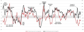


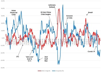
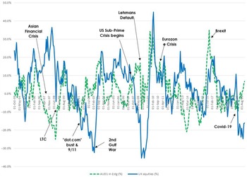

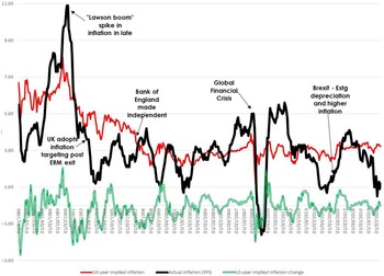


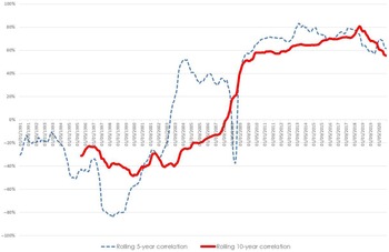
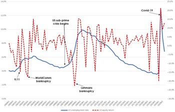
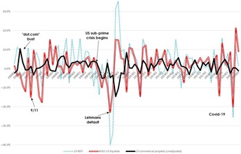
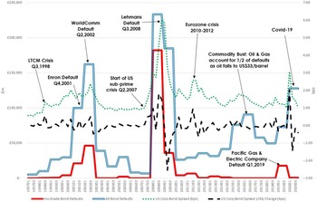
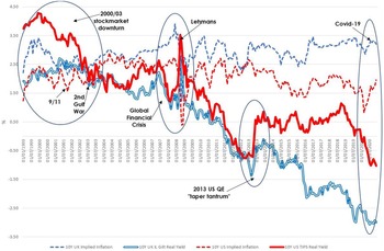
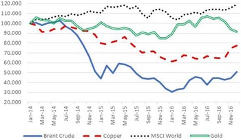
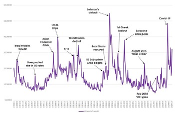

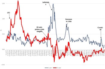

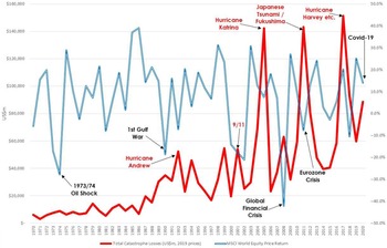


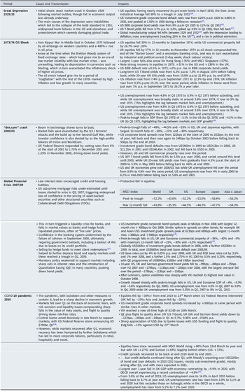
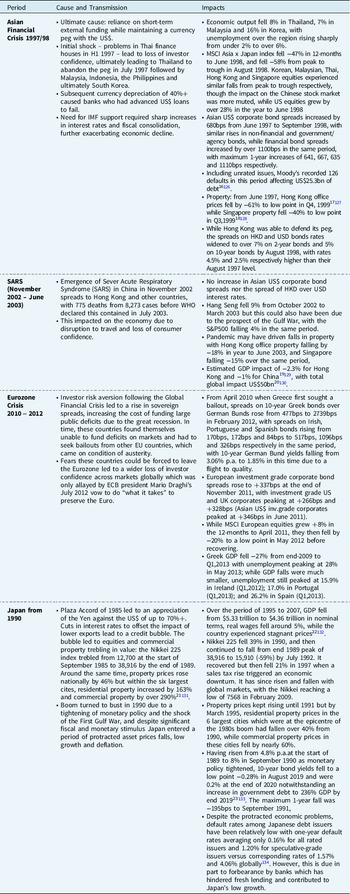

 Open access