


1. Introduction
Let  $\mathbb {H}^3$ denote the hyperbolic $3$-space, and let $G:=\operatorname {PSL}_2(\mathbb {C})$, which can be identified with the group $\operatorname {Isom}^+(\mathbb {H}^3)$ of all orientation preserving isometries of $\mathbb {H}^3$. Any complete orientable hyperbolic $3$-manifold can be presented as a quotient $M=\Gamma \backslash \mathbb {H}^3$ where $\Gamma$ is a torsion-free discrete subgroup of $G$. An oriented geodesic plane in $M$ is the image of a totally geodesic immersion of the hyperbolic plane $\mathbb {H}^2\subset \mathbb {H}^3$ equipped with an orientation under the quotient map $\mathbb {H}^3\to \Gamma \backslash \mathbb {H}^3$. In this paper, all geodesic planes are assumed to be oriented. Set $X:=\Gamma \backslash G$. Via the identification of $X$ with the oriented frame bundle $\operatorname {F}\! {{M}}$, a geodesic plane in $M$ arises as the image of a unique $\operatorname {PSL}_2(\mathbb {R})$-orbit under the base point projection map
 \[ \pi: X\simeq \operatorname{F}\! {{M}} \to {M}. \]
Moreover, a properly immersed geodesic plane in  $M$ corresponds to a closed $\operatorname {PSL}_2(\mathbb {R})$-orbit in $X$.
$X$.
Setting  $H:=\operatorname {PSL}_2(\mathbb {R})$, the main goal of this paper is to obtain a quantitative isolation result for closed $H$-orbits in $X$ when $\Gamma$ is a geometrically finite group. Fix a left invariant Riemannian metric on $G$, which projects to the hyperbolic metric on $\mathbb {H}^3$. This induces the distance $d$ on $X$ so that the canonical projection $G\to X$ is a local isometry. We use this Riemannian structure on $G$ to define the volume of a closed $H$-orbit in $X$. For a closed subset $S\subset X$ and ${\varepsilon }>0$, $B(S, {\varepsilon })$ denotes the ${\varepsilon }$-neighborhood of $S$.
$S$.
The case when  $M$ is compact

We first state the result for compact hyperbolic  $3$-manifolds. In this case, Ratner [Reference RatnerRat91] and Shah [Reference ShahSha91] independently showed that every $H$-orbit is either compact or dense in $X$. Moreover, there are only countably many compact $H$-orbits in $X$. Mozes and Shah [Reference Mozes and ShahMS95] proved that an infinite sequence of compact $H$-orbits becomes equidistributed in $X$. Our questions concern the following quantitative isolation property: for given compact $H$-orbits $Y\!$ and $Z$ in $X$,
$X$,
(1) How close can
$Y$ approach $Z$?(2) Given
${\varepsilon }>0$, what portion of $Y\!$ enters into the $\varepsilon$-neighborhood of $Z$?


It turns out that volumes of compact orbits are the only complexity which measures their quantitative isolation property. The following theorem was proved by Margulis in an unpublished note.
Theorem 1.1 (Margulis)
Let  $\Gamma$ be a cocompact lattice in $G$. For every $1/3\le s<1$, the following hold for any compact $H$-orbits $Y\ne Z$ in $X$.
$X$.
(1) We have
where\[ d(Y,Z )\gg \alpha_s^{-4/s} \cdot \operatorname{Vol}(Y)^{-1/s} \operatorname{Vol}(Z)^{-1/s} \]
$\alpha _s= ({1}/({1-s}))^{1/(1-s)}$.(2) For all
$0<\varepsilon < 1$,
where\[ m_{Y}(Y\cap B(Z, \varepsilon)) \ll \alpha_s^4 \cdot \varepsilon^{s} \cdot \operatorname{Vol}(Z) \]
$m_Y$ denotes the $H$-invariant probability measure on $Y$.


In both statements, the implied constants depend only on the injectivity radius of  $\Gamma \backslash G$ (see (A.9) and (A.10) for more details).
Remark 1.2 (1) By recent work [Reference Margulis and MohammadiMM22, Reference Bader, Fisher, Miller and StoverBFMS21], there may be infinitely many compact  $H$-orbits only when $\Gamma$ is an arithmetic lattice.
(2) Theorem 1.1 for some exponent  $s$ is proved in [Reference Einsiedler, Margulis and VenkateshEMV09, Lemma 10.3]. The proof in [Reference Einsiedler, Margulis and VenkateshEMV09] is based on the effective ergodic theorem which relies on the arithmeticity of $\Gamma$ via uniform spectral gap on compact $H$-orbits; the exponent $s$ obtained in their approach however is much smaller than $1$.
$1$.
(3) Margulis’ proof does not rely on the arithmeticity of  $\Gamma$ and is based on the construction of a certain function on $Y$ which measures the distance $d(y, Z)$ for $y\in Y$ (cf. (1.14)). A similar function appeared first in the work of Eskin, Mozes and Margulis in the study of a quantitative version of the Oppenheim conjecture [Reference Eskin, Margulis and MozesEMM98], and later in several other works (e.g. [Reference Eskin and MargulisEM04, Reference Benoist and QuintBQ12, Reference Eskin, Mirzakhani and MohammadiEMM15]).
General geometrically finite case
We now consider a general hyperbolic  $3$-manifold ${M}=\Gamma \backslash \mathbb {H}^3$. Denote by $\Lambda \subset \partial \mathbb {H}^3$ the limit set of $\Gamma$ and by ${\operatorname {core}}\, M$ the convex core of $M$, i.e.
 \[ {\operatorname{core}}\, M=\Gamma\backslash \operatorname{hull} \Lambda \subset M \]
where  $\operatorname {hull} \Lambda \subset \mathbb {H}^3$ denotes the convex hull of $\Lambda$. In the rest of the introduction, we assume that $M$ is geometrically finite, that is, the unit neighborhood of ${\operatorname {core}}\, M$ has finite volume.
Let  $Y\subset X$ be a closed $H$-orbit and $S_Y=\Delta _Y\backslash \mathbb {H}^2$ be the associated hyperbolic surface, where $\Delta _Y< H$ is the stabilizer in $H$ of a point in $Y$. We assume that $Y$ is non-elementary, that is, $\Delta _Y$ is not virtually cyclic; otherwise, we cannot expect an isolation phenomenon for $Y$, as there is a continuous family of parallel elementary closed $H$-orbits in general when $M$ is of infinite volume. It is known that $S_Y$ is always geometrically finite [Reference Oh and ShahOS13, Theorem 4.7].
Let  $0<\delta (Y)\le 1$ denote the critical exponent of $S_Y$, i.e. the abscissa of the convergence of the series $\sum _{\gamma \in \Delta _Y} e^{-s d(o, \gamma (o))}$ for some $o\in \mathbb {H}^2$. We define the following modified critical exponent of $Y$:
$Y$:
 \begin{equation} \delta_Y:=\begin{cases} \delta(Y) & \text{if $S_Y$ has no cusp,}\\ 2\delta(Y)-1 & \text{otherwise;}\end{cases} \end{equation}
note that  $0<\delta _Y\le \delta (Y) \le 1$, and $\delta _Y=1$ if and only if $S_Y$ has finite area.
In generalizing Theorem 1.1(1), we first observe that the distance  $d(Y, Z)$ between two closed $H$-orbits $Y, Z$ may be zero, e.g. if they both have cusps going into the same cuspidal end of $X$. To remedy this issue, we use the thick–thin decomposition of ${\operatorname {core}}\, M$. For $p\in M$, we denote by $\operatorname {inj} p$ the injectivity radius at $p$. For all ${\varepsilon }>0$, the ${\varepsilon }$-thick part
 \begin{equation} ({\operatorname{core}}\, M)_{{\varepsilon}}:=\{p\in {\operatorname{core}}\, M: \operatorname{inj} p\ge {\varepsilon}\} \end{equation}
is compact, and for all sufficiently small  ${\varepsilon }>0$, the ${\varepsilon }$-thin part given by ${\operatorname {core}}\, M-({\operatorname {core}}\, M)_{{\varepsilon }}$ is contained in finitely many disjoint cuspidal ends, i.e. images of horoballs in $\Gamma \backslash \mathbb {H}^3$. Let
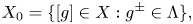
  $X_0\subset X$ denote the renormalized frame bundle $\operatorname {RF}\! {M}$ (see (2.1)). Using the fact that the projection of $X_0$ is contained in ${\operatorname {core}}\, M$ under $\pi$, we define the ${\varepsilon }$-thick part of $X_0$ as follows:
 \[ X_{{\varepsilon}}:=\{x\in X_0: \pi(x)\in ({\operatorname{core}}\, M)_{\varepsilon} \}. \]
The following theorem extends Theorem 1.1 to all geometrically finite hyperbolic manifolds.
Theorem 1.5 Let  ${M}$ be a geometrically finite hyperbolic $3$-manifold. Let $Y\ne Z$ be non-elementary closed $H$-orbits in $X$, and denote by $m_Y$ the probability Bowen–Margulis–Sullivan measure on $Y$. For every ${\delta _Y}/3\le s<\delta _Y$ the following hold.
(1) For all
$0<{\varepsilon } \ll 1$, we have
(1.6)where:\begin{equation} d (Y\cap X_\varepsilon, Z)\gg \alpha_{Y,s}^{-\star/s} \cdot \bigg(\frac{v_{Y,{\varepsilon}}}{\operatorname{area}_t Z} \bigg)^{1/s} \end{equation}•
$v_{Y,{\varepsilon }}=\min _{y\in Y\cap X_{\varepsilon }} {m_Y (B_Y(y, {\varepsilon }))}$ where $B_Y(y, {\varepsilon })$ is the ${\varepsilon }$-ball around $y$ in the induced metric on $Y$;•
$\operatorname {area}_t Z$ denotes the tight area of $S_Z$ relative to $M$ (Definition 1.7);•
$\alpha _{Y,s}:=\big ({{\mathsf {s}}_Y}/({ \delta _Y-s}\big )) ^{1/ (\delta _Y-s)}$ where $\mathsf {s}_Y\!$ is the shadow constant of $Y$ (Definition 1.8).
(2) For all
$0<{\varepsilon } \ll 1$,
\[ m_{Y}(Y\cap B(Z, {\varepsilon})) \ll \alpha_{Y,s}^\star \cdot {{\varepsilon}}^{s}\cdot \operatorname{area}_t Z. \]


In both statements, the implied constants and  $\star$ depend only on $\Gamma$.
Remark (1) We give a proof of a more general version of Theorem 1.5(1) where  $Z$ is allowed to be equal to $Y$ (see Corollary 10.5 for a precise statement).
(2) When  $X$ has finite volume, we have $\delta _Y=1$ and $m_Y$ is $H$-invariant so that $v_{Y, {\varepsilon }}\asymp {\varepsilon }^3 \operatorname {Vol} (Y)^{-1}$. Moreover, the tight area $\operatorname {area}_tZ$ and the shadow constant $\mathsf {s}_Y$ are simply the usual area of $S_Z$ and a fixed constant (in fact, the constant can be taken to be $2$) respectively. Therefore Theorem 1.5 recovers Theorem 1.1. Moreover, the exponent $\star$ depends only on $G$ as well; this follows since the proofs of Theorem 9.18 and theorems in § 10, of which Theorem 1.5 is a special case, show that $\star$ depends only on $\mathsf {s}_Y$, $\mathsf {p}_Y$ and $\delta _Y$, which are all absolute constants in the finite volume case.
We now give definitions of the tight area  $\operatorname {area}_t Z$ and the shadow constant $\mathsf {s}_Y$ for a general geometrically finite case; these are new geometric invariants introduced in this paper.
Definition 1.7 (Tight area of $S$)

For a properly immersed geodesic plane  $S$ of $M$, the tight-area of $S$ relative to $M$ is given by
 \[ \operatorname{area}_t(S):=\operatorname{area} (S\cap \mathcal{N}(\operatorname{core}\,M)) \]
where  $\mathcal{N}(\operatorname{core}\, M)=\{p\in M: d(p, q)\le \text {inj}(q)\text{ for some } q\in \operatorname{core}\, M\}$ is the tight neighborhood of ${\operatorname {core}}\, M$.
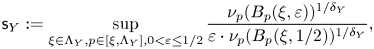
We show that  $\operatorname {area}_t(S)$ is finite in Theorem 3.3, by proving that $S\cap \mathcal { N}({\operatorname {core}}\, M)$ is contained in the union of a bounded neighborhood of ${\operatorname {core}}\, (S)$ and finitely many cusp-like regions (see Figure 1). We remark that the area of the intersection $S\cap B({\operatorname {core}}\, M, 1)$ is not finite in general.
Definition 1.8 (Shadow constant of $Y$)

For a closed  $H$-orbit $Y$ in $X$, let $\Lambda _Y\subset \partial \mathbb {H}^2$ denote the limit set of $\Delta _Y$, $\{\nu _{p}:p\in \mathbb {H}^2\}$ the Patterson–Sullivan density for $\Delta _Y$, and $B_p(\xi, {\varepsilon })$ the ${\varepsilon }$-neighborhood of $\xi \in \partial \mathbb {H}^2$ with respect to the Gromov metric at $p$. The shadow constant of $Y$ is defined as follows:
 \begin{equation} \mathsf{s}_Y:=\sup_{\xi\in \Lambda_Y, p\in [ \xi,\Lambda_Y], 0< {\varepsilon}\le 1/2} \frac{\nu_{p}(B_p(\xi,{\varepsilon}))^{1/\delta_Y}}{{\varepsilon}\cdot \nu_p(B_p(\xi, 1/2))^{1/\delta_Y}}, \end{equation}
where  $[\xi, \Lambda _Y]$ is the union of all geodesics connecting $\xi$ to a point in $\Lambda _Y$.
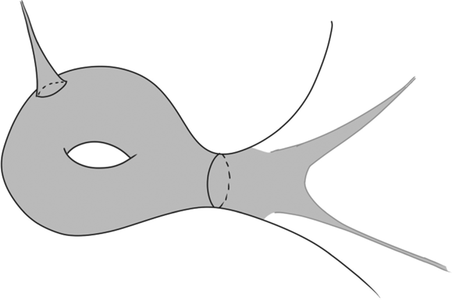
Figure 1.  $S\cap \mathcal {N}({\operatorname {core}}\, M)$.
We show that  $\mathsf {s}_Y<\infty$ in Theorem 4.8.
Remark 1.10 If  $Y$ is convex cocompact, then for all $0<{\varepsilon }<1$, we have $v_{Y, {\varepsilon }}\asymp {\varepsilon }^{1+2\delta _Y}$ with the implied constant depending on $Y$. When $Y$ has a cusp, Sullivan's shadow lemma (cf. Proposition 4.11) implies that $\lim _{{\varepsilon }\to 0} {\log v_{Y, {\varepsilon }}}/{\log {\varepsilon }}$ does not exist.
A hyperbolic  $3$-manifold ${M}$ is called convex cocompact acylindrical if ${\operatorname {core}}\, M$ is a compact manifold with no essential discs or cylinders which are not boundary parallel. For such a manifold, there exists a uniform positive lower bound for $\delta (Y)=\delta _Y$ for all non-elementary closed $H$-orbits $Y$ [Reference McMullen, Mohammadi and OhMMO17]; therefore the dependence of $\delta _Y$ can be removed in Theorem 1.5 if one is content with taking some $s$ which works uniformly for all such orbits.
Examples of  $X$ with infinitely many closed $H$-orbits are provided by the following theorem which can be deduced from [Reference McMullen, Mohammadi and OhMMO17, Reference McMullen, Mohammadi and OhMMO22, Reference Benoist and OhBO22].
Theorem 1.11 Let  ${M}_0$ be an arithmetic hyperbolic $3$-manifold with a properly immersed geodesic plane. Any geometrically finite acylindrical hyperbolic $3$-manifold ${M}$ which covers ${M}_0$ contains infinitely many non-elementary properly immersed geodesic planes.
It is easy to construct examples of  ${M}$ satisfying the hypothesis of this theorem. For instance, if ${M}_0$ is an arithmetic hyperbolic $3$-manifold with a properly embedded compact geodesic plane $P$,
$P$,  ${M}_0$ is covered by a geometrically finite acylindrical manifold ${M}$ whose convex core has boundary isometric to $P$.
$P$.
Finally, we mention the following application of Theorem 1.5 in view of recent interests in related counting problems [Reference Calegari, Marques and NevesCMN22].
Corollary 1.12 Let  $\operatorname {Vol}(M)<\infty$, and let $\mathcal {N}(T)$ denote the number of properly immersed totally geodesic planes $P$ in $M$ of area at most $T$. Then for any $1/2< s<1$, we have
 \[ \mathcal{N}(T) \ll_sT^{(6/s)-1}\quad \text{ for all $T>1$}; \]
see Corollary 10.7 for a detailed information on the dependence of the implied constant.
We remark that when  $\operatorname {Vol} (M)<\infty$, the heuristics suggest $s={\operatorname {dim} G/ H}=3$ in Theorem 1.5 and hence $\mathcal {N}(T)\ll T$ in Corollary 1.12. Indeed, when $\Gamma =\operatorname {PSL}_2 (\mathbb {Z}[i])$, the asymptotic $\mathcal {N}(T)\sim c \cdot T$, as suggested in [Reference SarnakSar05], has been obtained by Jung [Reference JungJun19] based on subtle number theoretic arguments.
Remark 1.13 We can also obtain an estimate for  $\mathcal {N}(T)$ for a general geometrically finite hyperbolic manifold. By [Reference McMullen, Mohammadi and OhMMO17, Reference Benoist and OhBO22], if $\operatorname {Vol} (M)=\infty$, there are only finitely many properly immersed geodesic planes of finite area (note that they are necessarily contained in the convex core of $M$); hence $\sup _{T} \mathcal {N}(T) <\infty$. We also obtain that there exists $N_0\ge 1$ (depending only on $G$) such that for any $1/2< s<1$, we have
 \[ \mathcal{N}(T)\ll_s \operatorname{Vol} (\text{unit-nbd of core}\ M)\, {\varepsilon}_M^{-N_0} T^{{6}/{s}-1} \]
where the implied constant depends only on  $s$ (see Remark 10.11 for details). Note that this kind of upper bound is meaningful despite the finiteness result mentioned above, as the implied constant is independent of $M$.
$M$.
Discussion on proofs
We discuss some of the main ingredients of the proof of Theorem 1.5. First consider the case when  $X=\Gamma \backslash G$ is compact (the account below deviates slightly from Margulis’ original argument). Let ${\varepsilon }_X$ be the minimum injectivity radius of points in $X$. The Lie algebra of $G$ decomposes as $\mathfrak {sl}_2(\mathbb {R}) \oplus i\mathfrak {sl}_2(\mathbb {R})$. Hence, for each $y\in Y$, the set
 \[ I_Z(y):=\{v\in i\mathfrak{sl}_2(\mathbb{R}): 0<\|v\| <{\varepsilon}_X,\ y\exp(v)\in Z\} \]
keeps track of all points of  $Z\cap B(y, {\varepsilon }_X)$ in the direction transversal to $H$ (see Figure 2).
Figure 2.  $I_Z(y)$.
Therefore, the following function  $f_s:Y\to [2,\infty )$ ( $0< s<1$) encodes the information on the distance $d(y, Z)$:
 \begin{equation} f_s(y)=\begin{cases} \sum_{v\in I_Z(y)}\|v\|^{-s} & \text{if $I_Z(y)\neq\emptyset $},\\ {\varepsilon}_X^{-s} & \text{otherwise.} \end{cases} \end{equation}
A function of this type is referred to as a Margulis function in the literature.
The proof of Theorem 1.1 is based on the following fact: the average of  $f_s$ is controlled by the volume of $Z$, i.e.
 \begin{equation} m_Y(f_s)\ll_s \operatorname{Vol}(Z). \end{equation}
 We prove the estimate in (1.15) using the following super-harmonicity type inequality: for any  $1/3\le s<1$, there exist $t=t_s>0$ and $b=b_s>1$ such that for all $y\in Y$,
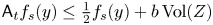 \begin{equation} {\mathsf{A}}_t f_s(y) \le \tfrac{1}{2} f_s(y)+ b\operatorname{Vol}(Z) \end{equation}
where  $({\mathsf {A}}_t f_s)(y)= \int _0^1 f_s(yu_ra_t)\,dr$, $u_r=\bigl (\begin {smallmatrix} 1 & 0\\r & 1\end {smallmatrix}\bigr )$, and $a_t=\bigl (\begin {smallmatrix} e^{t/2} & 0\\0 & e^{-t/2}\end {smallmatrix}\bigr )$.
The proof of (1.16) is based on the inequality (A.1), which is essentially a lemma in linear algebra. We refer to Appendix A, where a more or less complete proof of Theorem 1.1 is given.
For a general geometrically finite hyperbolic manifold, many changes are required, and several technical difficulties arise. In general, there is no positive lower bound for the injectivity radius on  $X$, and the shadow constant of $Y$ appears in the linear algebra lemma (Lemma 5.6). These facts force us to incorporate the height of $y$ as well as the shadow constant of $Y$ in the definition of the Margulis function (see Definition 9.1). The correct substitutes for the volume measures on $Y$ and $Z$ turn out to be the Bowen–Margulis–Sullivan probability measure $m_Y$ and the tight area of $Z$ respectively.
It is more common in the existing literature on the subject to define the operator  ${\mathsf {A}}_t$ using averages over large spheres in $\mathbb {H}^2$. Our operator ${\mathsf {A}}_t$, however, is defined using averages over expanding horocyclic pieces; this choice is more amenable to the change of variables and iteration arguments for Patterson–Sullivan measures. Indeed, for a locally bounded Borel function $f$ on $Y\cap X_0$ and for any $y\in Y\cap X_0$,
 \[ ({\mathsf{A}}_t f)(y)= \frac{1}{\mu_y([-1,1])}\int_{-1}^1 f(yu_ra_t)\,d\mu_y(r) \]
where  $\mu _y$ is the Patterson–Sullivan measure on $yU$ (see (4.2)).
When  $X$ is compact and hence $m_Y$ is $H$-invariant, (1.15) follows by simply integrating (1.16) with respect to $m_Y$. In general, we resort to Lemma 7.3, the proof of which is based on an iterated version of (1.16) for ${\mathsf {A}}_{nt_0}$, $n\in \mathbb {N}$, for some $t_0>0$, as well as on the fact that the Bowen–Margulis–Sullivan measure $m_Y$ is $a_{t_0}$-ergodic.
In fact, the main technical result of this paper can be summarized as follows.
Proposition 1.17 Let  $\Gamma$ be a geometrically finite subgroup of $G$. Let $Y\ne Z$ be non-elementary closed $H$-orbits in $X=\Gamma \backslash G$, and set $Y_0:=Y\cap X_0$. For any $ { \delta _Y}/{3} \le s<\delta _Y$, there exist $t_s>0$ and a locally bounded Borel function $F_s:Y_0\to (0, \infty )$ with the following properties.
(1) For all
$y\in Y_0$,
\[ d(y, Z) ^{-s}\le \mathsf{s}_Y^{\star} F_s(y). \]
(2) For all
$y\in Y_0$ and $n\ge 1$,
\[ \big({\mathsf{A}}_{nt_s} F_s\big) (y)\le \frac{1}{2^{n}} F_{s}(y)+ \alpha_{Y,s}^\star \operatorname{area}_t(S_Z). \]
(3) There exists
$1< \sigma \ll {\mathsf {s}}_Y^{\star }$ such that for all $y\in Y_0$ and for all $h\in H$ with $\|h\|\ge 2$ and $yh\in Y_0$,
\[ \sigma^{-1} F_{s} (y) \le F_{s}(yh) \le \sigma F_{s}(y). \]


Finally we mention that the reason that we can take the exponent  $s$ arbitrarily close to $\delta _Y$ lies in the two ingredients of our proof: first, the linear algebra lemma (Lemma 5.6) is obtained for all $\delta _Y/3\le s<\delta _Y$; and second, for any $y\in Y\cap X_0$, we can find $|r|<1$ so that $yu_r\in X_0$ and the height of $yu_r$ can be lowered to be $O(1)$ by the geodesic flow of time comparable to the logarithmic height of $y$; see Lemma 8.4 for the precise statement.
Organization
We end this introduction with an outline of the paper. In §2, we fix some notation and conventions to be used throughout the paper. In § 3, we show the finiteness of the tight area of a properly immersed geodesic plane. In § 4, we show the finiteness of the shadow constant of a closed  $H$-orbit. In § 5, we prove a lemma from linear algebra; this lemma is a key ingredient to prove a local version of our main inequality. Section 6 is devoted to the study of the height function in $X_0$. In § 7, the definition of the Markov operator and a basic property of this operator are discussed. In § 8, we prove the return lemma, and use it to obtain a uniform control on the number of sheets of $Z$ in a neighborhood of $y$. In § 9, we construct the desired Margulis function and prove the main inequalities. In § 10, we give a proof of Theorem 1.5. In Appendix A, we provide a proof of Theorem 1.1.
2. Notation and preliminaries
In this section, we review some definitions and introduce notation which will be used throughout the paper.
We set  $G=\operatorname {PSL}_2(\mathbb {C})\simeq \operatorname {Isom}^+(\mathbb {H}^3)$, and $H=\operatorname {PSL}_2(\mathbb {R})$. We fix $\mathbb {H}^2\subset \mathbb {H}^3$ with an orientation so that $\{g\in G: g(\mathbb {H}^2)=\mathbb {H}^2\}=H$. Let $A$ denote the following one-parameter subgroup of $G$:
$G$:
 \[ A=\bigg\{ a_t=\begin{pmatrix} e^{t/2} & 0 \\ 0 & e^{-t/2} \end{pmatrix} : t\in \mathbb{R} \bigg\}. \]
Set  $K_0=\operatorname {PSU}(2)$ and $M_0$ the centralizer of $A$ in $K_0$. We fix a point $o\in \mathbb {H}^2\subset \mathbb {H}^3$ and a unit tangent vector $v_{o}\in \operatorname {T}_{o}(\mathbb {H}^3)$ so that their stabilizer subgroups are $K_0$ and $M_0$ respectively. The isometric action of $G$ on $\mathbb {H}^3$ induces identifications $G/K_0=\mathbb {H}^3$, $G/M_0=\operatorname {T}^1 \mathbb {H}^3$, and $G=\operatorname {F}\mathbb {H}^3$ where $\operatorname {T}^1 \mathbb {H}^3$ and $\operatorname {F}\! \mathbb {H}^3$ denote, respectively, the unit tangent bundle and the oriented frame bundle over $\mathbb {H}^3$. Note also that $H\cap K_0=\operatorname {PSO(2)}$ and that $H(o)= \mathbb {H}^2$.
The right translation action of  $A$ on $G$ induces the geodesic/frame flow on $\operatorname {T}^1 \mathbb {H}^3$ and $\operatorname {F}\! \mathbb {H}^3$, respectively. Let $v_{o}^{\pm }\in \partial \mathbb {H}^3$ denote the forward and backward end points of the geodesic given by $v_{o}$. For $g\in G$, we define
 \[ g^{\pm}:=g(v_{o}^{\pm})\in \partial \mathbb{H}^3 . \]
Let  $\Gamma < G$ be a discrete torsion-free subgroup. We set
 \[ {M}:=\Gamma\backslash \mathbb{H}^3\quad \text{ and } \quad X:=\Gamma\backslash G\simeq \operatorname{F}\! M. \]
We denote by  $\pi : X\to M$ the base point projection map. Denote by $\Lambda =\Lambda (\Gamma )$ the limit set of $\Gamma$. The convex core of $M$ is given by ${\operatorname {core}}\, M=\Gamma \backslash \text {hull} (\Lambda )$. Let $X_0$ denote the renormalized frame bundle $\operatorname {RF}\! {M}$, i.e.
 \begin{equation} X_0=\{[g]\in X: g^{\pm}\in \Lambda\} , \end{equation}
that is,  $X_0$ is the union of all the $A$-orbits whose projections to $M$ stay inside ${\operatorname {core}}\, M$. We remark that $X_0$ does not surject onto ${\operatorname {core}}\, M$ in general.
In the whole paper, we assume that  $\Gamma$ is geometrically finite, that is, the unit neighborhood of ${\operatorname {core}}\, M$ has finite volume. This is equivalent to the condition that $\Lambda$ is the union of the radial limit points and bounded parabolic limit points: $\Lambda =\Lambda _{\rm rad}\bigcup \Lambda _{\rm bp}$ (cf. [Reference BowditchBow93, Reference Matsuzaki and TaniguchiMT98]). A point $\xi \in \Lambda$ is called radial if the projection of a geodesic ray toward to $\xi$ accumulates on $M=\Gamma \backslash \mathbb {H}^3$, parabolic if it is fixed by a parabolic element of $\Gamma$, and bounded parabolic if it is parabolic and $\operatorname {Stab}_\Gamma (\xi )$ acts co-compactly on $\Lambda -\{\xi \}$. In particular, for $\Gamma$ geometrically finite, the set of parabolic limit points $\Lambda _{\rm p}$ is equal to $\Lambda _{\rm bp}$. For $\xi \in \Lambda _{\rm p}$, the rank of the free abelian subgroup $\operatorname {Stab}_\Gamma (\xi )$ is referred to as the rank of $\xi$.
A geometrically finite group  $\Gamma$ is called convex cocompact if ${\operatorname {core}}\, M$ is compact, or equivalently, if $\Lambda =\Lambda _{\rm rad}$.
We denote by  $N$ the expanding horospherical subgroup of $G$ for the action of $A$:
$A$:
 \[ N =\left\{u_s=\begin{pmatrix} 1 & 0 \\ s & 1\end{pmatrix}: s\in \mathbb{C} \right\}. \]
For  $\xi \in \Lambda _{\rm p}$, a horoball $\tilde {\mathfrak {h}}_{\xi }\subset G$ based at $\xi$ is of the form
 \begin{equation} \tilde{\mathfrak{h}}_\xi(T) =g N { A}_{( -\infty, -T]} K_0 \quad \text{for some $T\ge 1$,} \end{equation}
where  $g\in G$ is such that $g^-=\xi$ and ${A}_{(-\infty,-T]}=\{a_{t}: -\infty < t\le -T\}$. Its image $\tilde {\mathfrak {h}}_\xi (o)$ in $\mathbb {H}^3$ is called a horoball in $\mathbb {H}^3$ based at $\xi$. By a horoball $\mathfrak {h}_\xi$ in $X$ and in $M$, we mean their respective images of horoballs $\tilde {\mathfrak {h}}_{\xi }$ and $\tilde {\mathfrak {h}}_\xi (o)$ in $X$ and $M$ under the corresponding projection maps.
Thick–thin decomposition of $X_0$

We fix a Riemannian metric  $d$ on $G$ which induces the hyperbolic metric on $\mathbb {H}^3$. By abuse of notation, we use $d$ to denote the distance function on $X$ induced by $d$, as well as on $M$. For a subset $S\subset \spadesuit$ and ${\varepsilon }>0$, $B_\spadesuit (S, {\varepsilon })$ denotes the set $\{x\in \spadesuit : d(x, S)\le {\varepsilon }\}$. When $\spadesuit$ is a subgroup of $G$ and $S=\{e\}$, we simply write $B_\spadesuit ({\varepsilon })$ instead of $B_\spadesuit (S, {\varepsilon })$. When there is no room for confusion for the ambient space $\spadesuit$, we omit the subscript $\spadesuit$.
For  $p\in M$, we denote by $\operatorname {inj} p$ the injectivity radius at $p\in M$, that is: the supremum $r>0$ such that the projection map $\mathbb {H}^3\to M=\Gamma \backslash \mathbb {H}^3$ is injective on the ball $B_{\mathbb {H}^3}(\tilde p, r)$ where $\tilde p\in \mathbb {H}^3$ is such that $p=[\tilde p]=\tilde p\Gamma$. For $S\subset M$ and ${\varepsilon }>0$, we call the subsets $\{p\in S: \operatorname {inj} (p)\ge {\varepsilon }\}$ and $\{p\in S: \operatorname {inj} (p)< {\varepsilon }\}$ the ${\varepsilon }$-thick part and the ${\varepsilon }$-thin part of $S$ respectively.
As  $M$ is geometrically finite, ${\operatorname {core}}\, M$ is contained in a union of its ${\varepsilon }$-thick part $({\operatorname {core}}\, M)_{\varepsilon }$ and finitely many disjoint horoballs for all small ${\varepsilon }>0$ (cf. [Reference Matsuzaki and TaniguchiMT98]). If $p=gu_sa_{-t}o$ is contained in a horoball $\mathfrak {h}_\xi = g N {A}_{( -\infty, -T]}(o)$, then $\operatorname {inj} (p)\asymp e^{-t}$ for all $t\gg T$, this is a standard fact see, e.g. [Reference Kelmer and OhKO21, Proposition 5.1].
Let  ${\varepsilon }_M>0$ be the supremum of ${\varepsilon }$ with respect to which such a decomposition of ${\operatorname {core}}\, M$ holds. We call the ${\varepsilon }_M$-thick part of ${\operatorname {core}}\, M$ the compact core of $M$, and denote by $M_{{\rm cpt}}$.
For  $x=[g]\in X$, we denote by $\operatorname {inj}(x)$ the injectivity radius of $\pi (x)\in M$. For $\varepsilon >0$, we set
 \[ X_\varepsilon:=\{x\in X_0:\operatorname{inj} (x) \ge {\varepsilon}\}. \]
We set  ${\varepsilon }_X={\varepsilon }_M/2$; note that $X_0-X_{{\varepsilon }_X}$ is either empty or is contained in a union of horoballs in $X$.
$X$.
Convention
By an absolute constant, we mean a constant which depends at most on  $G$ and $\Gamma$. We will use the notation $A\asymp B$ when the ratio between the two lies in $[C^{-1}, C]$ for some absolute constant $C\ge 1$. We write $A\ll B^\star$ (respectively $A\asymp B^\star$, $A\ll \star B$) to mean that $A\le C B^L$ (respectively $C^{-1}B^L\le A\le C B^L$, $A\le C\cdot B$) for some absolute constants $C>0$ and $L>0$.
3. Tight area of a properly immersed geodesic plane
In this section, we show that the tight area of a properly immersed geodesic plane of  $M$ is finite.
For a closed subset  $Q\subset M$, we define the tight neighborhood of $Q$ by
 \[ \mathcal{N}(Q):=\{p\in M: d(p, q)\le \text{inj}(q)\text{ for some $q\in Q$} \}. \]
We are mainly interested in the tight neighborhood of  ${\operatorname {core}}\, M$. If $M$ is convex cocompact, $\mathcal {N}({\operatorname {core}}\, M)$ is compact. In order to describe the shape of $\mathcal {N}({\operatorname {core}}\, M)$ in the presence of cusps, fix a set $\xi _1, \ldots, \xi _\ell$ of $\Gamma$-representatives of $\Lambda _{\rm p}$, cf. [Reference Matsuzaki and TaniguchiMT98]. Then ${\operatorname {core}}\, M$ is contained in the union of $M_{\rm cpt}$ and a disjoint union $\bigcup \mathfrak {h}_{\xi _i}$ of horoballs based at the $\xi _i$s.
Consider the upper half-space model  $\mathbb {H}^3=\{(x_1, x_2,y): y>0\}=\mathbb {R}^2\times \mathbb {R}_{>0}$, and let $\infty \in \Lambda _{\rm p}$. Let $p:\mathbb {H}^3\to M$ denote the canonical projection map. As $\infty$ is a bounded parabolic fixed point, there exists a bounded rectangle, say, $I\subset \mathbb {R}^2$ and $r>0$ (depending on $\infty$) such that:
(1)
$p(I\times \{y> r \})\supset \mathcal {N}(\mathfrak {h}_\infty \cap {\operatorname {core}}\, M)$; and(2)
$p( I\times \{r\})\subset B(M_{\rm cpt}, R)$


where  $R$ depends only on $M$. We call this set $\mathfrak {C}_\infty :=I\times \{y\ge r \}$ a chimney for $\infty$ (cf. Figure 3).

Figure 3. Chimney.
Note that increasing  $R$ if necessary, we have
 \begin{equation} \mathcal{N}({\operatorname{core}}\, M)\subset B(M_{\rm cpt}, R) \cup \biggl(\bigcup_{1\le i\le \ell} p(\mathfrak{C}_{\xi_i})\biggr), \end{equation}
where  $\mathfrak {C}_{\xi _i}$ is a chimney for $\xi _i$.
Definition 3.2 For a properly immersed geodesic plane  $S$ of $M$, we define the tight-area of $S$ relative to $M$ as follows:
 \[ \operatorname{area}_t(S):=\operatorname{area} (S\cap \mathcal{N}({\operatorname{core}}\, M)). \]
Theorem 3.3 For a properly immersed non-elementary geodesic plane  $S$ of $M$, we have
 \[ 1\ll \operatorname{area}_t(S) <\infty, \]
where the implied multiplicative constant depends only on  $M$.
$M$.
Proof. Since no horoball can contain a complete geodesic, it follows that  $S$ intersects the compact core $M_{{\rm cpt}}$. Therefore,
 \[ \operatorname{area}_t S\ge 4\pi\sinh^2({\varepsilon}_X/2), \]
as  $S\cap M_{\rm cpt}$ contains a hyperbolic disk of radius ${\varepsilon }_X$ (see § 2). This implies the lower bound.
We now turn to the proof of the upper bound. We use the notation in (3.1). Fix a geodesic plane  $P\subset \mathbb {H}^3$ which covers $S$ and let $\Delta ={\rm Stab}_\Gamma (P)$. Fix a Dirichlet domain $D$ in $P$ for the action of $\Delta$. As $\Delta \backslash P$ is geometrically finite, the Dirichlet domain is a finite sided polygon; hence, $D\cap \operatorname {hull} (\Delta )$ has finite area, and the set $D-\operatorname {hull} (\Delta )$ is a disjoint union of finitely many flares, where a flare is a region bounded by three geodesics as shown in Figure 4. Fixing a flare $F\subset D-\operatorname {hull} (\Delta )$, it suffices to show that $\{x\in F: p(x)\in \mathcal {N} ({\operatorname {core}}\, M)\}$ has finite area. As $S$ is properly immersed, the set $\{x\in F: d(p(x), M_{\rm cpt})\le R\}$ is bounded. Therefore, fixing a chimney $\mathfrak {C}_{\xi _i}$ as above, it suffices to show that the set $\{x\in F: p(x)\in \mathfrak {C}_{\xi _i}\}=F\cap \Gamma \mathfrak {C}_{\xi _i}$ has finite area.
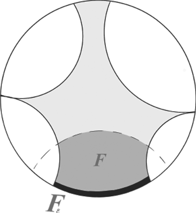
Figure 4. Flare  $F$ and $F_{\varepsilon }$.
Without loss of generality, we may assume  $\xi _i=\infty$. We will denote by $\partial F$ the intersection of the closure of $F$ and $\partial P$, and let $F_{\varepsilon }\subset \overline {F}$ denote the ${\varepsilon }$-neighborhood of $\partial F$ in the Euclidean metric in the unit disc model of $\overline {P}$ (cf. Figure 4).
Fix  ${\varepsilon }_0>0$ so that
 \begin{equation} F_{{\varepsilon}_0}\cap \{x\in D: d(p(x), M_{\rm cpt})< R\}=\emptyset; \end{equation}
such  ${\varepsilon }_0$ exists, as $S$ is a proper immersion. Writing $\mathfrak {C}_\infty =I\times \{y\ge r\}$ as above, let $H_\infty :=\mathbb {R}^2\times \{y>r\}$, and set $\Gamma _\infty :=\operatorname {Stab}_\Gamma (\infty )$.
We claim that
 \begin{equation} \#\{\gamma H_\infty: F_{{\varepsilon}_0/2}\cap \gamma \mathfrak{C}_\infty\ne \emptyset\}<\infty. \end{equation}
Suppose not. Since  $\Gamma H_\infty$ is closed in the space of all horoballs in $\mathbb {H}^3$, there exists a sequence of distinct $\gamma _i(\infty )\in \Gamma (\infty )$ such that $F_{{\varepsilon }_0/2}\cap \gamma _i \mathfrak {C}_\infty \ne \emptyset$ and the size of the horoballs $\gamma _i H_\infty$ goes to $0$ in the Euclidean metric in the ball model of $\mathbb {H}^3$. Note that if $\infty$ has rank $2$, then $\Gamma _\infty (I\times \{r\})=\mathbb {R}^2\times \{r\}$ and that if $\infty$ has rank $1$, then $\Gamma _\infty (I\times \{r\})$ contains a region between two parallel horocycles in $\mathbb {R}^2\times \{r\}$. Since $P\cap \gamma _i \mathfrak {C}_\infty \ne \emptyset$, it follows that $P\cap \gamma _i (\Gamma _\infty (I \times \{r\})) \ne \emptyset$. Moreover, if $i$ is large enough so that the Euclidean size of $\gamma _i H_\infty$ is smaller than ${\varepsilon }_0/2$, the condition $F_{{\varepsilon }_0/2} \cap \gamma _i \mathfrak {C}_\infty \ne \emptyset$ implies that $F_{{\varepsilon }_0} \cap \gamma _i (\Gamma _\infty (I \times \{r\})) \ne \emptyset$. This yields a contradiction to (3.4) since $p(I\times \{r\})$ is contained in the $R$-neighborhood of $M_{\rm cpt}$, proving the claim.
By Claim 3.5, it is now enough to show that, fixing a horoball  $\gamma H_\infty$, the intersection $F_{{\varepsilon }_0}\cap \gamma \Gamma _\infty \mathfrak {C}_\infty$ has finite area. Suppose that $F_{{\varepsilon }_0}\cap \gamma \Gamma _\infty \mathfrak {C}_\infty$ is unbounded in $P$; otherwise the claim is clear. Without loss of generality, we may assume $\gamma =e$, by replacing $P$ by $\gamma ^{-1}P$ if necessary. If $\infty \notin \partial P$, then $F_{{\varepsilon }_0}\cap \Gamma _\infty \mathfrak {C}_\infty$, being contained in $P\cap H_\infty$, is a bounded subset of $P$, which contradicts our supposition. Therefore, $\infty \in \partial P$. Then, as $F_{{\varepsilon }_0}\cap \Gamma _\infty \mathfrak {C}_\infty \subset F_{{\varepsilon }_0}\cap H_\infty$ is unbounded, we have $\infty \in \partial F$. Since $F$ is a flare, it follows that $\infty$ is not a limit point for $\Delta$. This implies that the rank of $\infty$ in $\Lambda _{\rm p}$ is $1$ [Reference Oh and ShahOS13, Lemma 6.2]. Therefore $\Gamma _\infty \mathfrak {C}_\infty$ is contained in a subset of the form $T\times \{y\ge r\}$ where $T$ is a strip between two parallel lines $L_1, L_2$ in $\mathbb {R}^2$. Since $\infty$ is not a limit point for $\Delta$, the vertical plane $P$ is not parallel to the $L_i$. Therefore, the intersection $F_{{\varepsilon }_0}\cap \Gamma _\infty \mathfrak {C}_\infty$, being a subset of $P\cap (T\times \{y\ge r\})$, is contained in a cusp-like region, isometric to $\{(x,y)\in \mathbb {H}^2: y\ge r\}$ and $x$ is also bounded from above and below (recall that $P$ is not parallel to the $L_i$). This finishes the proof.
The proof of the above theorem demonstrates that the portion of  $S$, especially of the flares of $S$, staying in the tight neighborhood of ${\operatorname {core}}\, M$ can go to infinity only in cusp-like shapes, by visiting the chimneys of horoballs of ${\operatorname {core}}\, M$ (Figure 1). This is not true any more if we replace the tight neighborhood of ${\operatorname {core}}\, M$ by the unit neighborhood of ${\operatorname {core}}\, M$. More precisely if $\Lambda$ contains a parabolic limit point of rank one which is not stabilized by any element of $\pi _1(S)$, then some region of $S$ with infinite area can stay inside the unit neighborhood of ${\operatorname {core}}\, M$. This situation may be compared to the presence of divergent geodesics in finite area setting.
4. Shadow constants
In this section, fixing a closed non-elementary  $H$-orbit $Y$ in $X$, we recall the definition of Patterson–Sullivan measures $\mu _y$ on horocycles in $Y$, and relate its density with the shadow constant $\mathsf {s}_Y$, which we show is a finite number.
Set  $\Delta _Y:=\operatorname {Stab}_H(y_0)$ to be the stabilizer of a point $y_0\in Y$; note that despite the notation, $\Delta _Y$ is uniquely determined up to a conjugation by an element of $H$. As $\Gamma$ is geometrically finite and $Y=Hy_0$ is a closed orbit, the subgroup $\Delta _Y$ is a geometrically finite subgroup of $H$, [Reference Oh and ShahOS13, Theorem 4.7]. We denote by $\Lambda _Y\subset \partial \mathbb {H}^2$ the limit set of $\Delta _Y$. Let $0<\delta (Y)\le 1$ denote the critical exponent of $\Delta _Y$, or equivalently, the Hausdorff dimension of $\Lambda _Y$.
We denote by  $\{\nu _p=\nu _{Y, p}: p\in \mathbb {H}^2\}$ the Patterson–Sullivan density for $\Delta _Y$, normalized so that $|\nu _o|=1$. This means that the collection $\{\nu _p\}$ consists of Borel measures on $\Lambda _Y$ satisfying that for all $\gamma \in \Delta _Y$, $p, q \in \mathbb {H}^2$, $\xi \in \Lambda _Y$,
 \[ \frac{d \gamma_* \nu_p}{d\nu_p}(\xi) =e^{-\delta(Y) \beta_\xi(\gamma^{-1}(p), p)}\quad \text{and}\quad \frac{d \nu_q}{d\nu_p}(\xi) =e^{-\delta(Y) \beta_\xi(q, p)} \]
where  $\beta _\xi (\cdot, \cdot )$ denotes the Busemann function. In what follows we will refer to the first identity above as $\Gamma$-conformality of $\{\nu _p\}$.
As  $\Delta _Y\!$ is geometrically finite, there exists a unique Patterson–Sullivan density up to a constant multiple.
PS-measures on $U$-orbits

Set
 \[ U :=\bigg\{u_r=\begin{pmatrix} 1 & 0 \\ r & 1\end{pmatrix}: r\in \mathbb{R} \bigg\}=N\cap H \]
which is the expanding horocylic subgroup of  $H$. Using the parametrization ${r}\mapsto u_{r}$, we may identify $U$ with $\mathbb {R}$. Note that for all $r,t\in \mathbb {R}$,
 \[ a_{-t}u_{r} a_t=u_{e^t{r}}. \]
For any  $h\in H$, the restriction of the visual map $g\mapsto g^+$ is a diffeomorphism between $hU$ and $\partial \mathbb {H}^2-\{h^-\}$. Using this diffeomorphism, we can define a measure $\mu _{hU}$ on $hU$:
$hU$:
 \begin{equation} d \mu_{hU} (hu_{r} )= e^{\delta(Y) \beta_{(hu_{{r}})^+}(p,hu_{{r}}(p))} \,d{\nu_{p}}(hu_{{r}})^+ ; \end{equation}
this is independent of the choice of  $p\in \mathbb {H}^2$. We simply write $d\mu _{h}({r})$ for $d \mu _{hU} (hu_{r} )$. Note that these measures depend on the $U$-orbits but not on the individual points. By the $\Delta _Y$-invariance and the conformal property of the PS-density, we have
 \begin{equation} d\mu_h (\mathcal{O})=d\mu_{\gamma h} (\mathcal{O}) \end{equation}
for any  $\gamma \in \Delta _Y$ and for any bounded Borel set $\mathcal {O}\subset \mathbb {R}$; therefore $\mu _{y}(\mathcal {O})$ is well defined for $y\in \Delta _Y\backslash H$.
For any  $y\in \Delta _Y\backslash H$ and any $t\in \mathbb {R}$, we have
 \begin{equation} \mu_y([-e^t,e^t])=e^{\delta(Y) t}\mu_{ya_{-t}}([-1,1]). \end{equation}
Set
 \begin{equation} Y_0:=\{[h]\in \Delta_Y\backslash H: h^{\pm}\in \Lambda_Y\} \end{equation}
where  $h^{\pm }= \lim _{t\to \pm \infty } ha_t(o)$.
Shadow constant
As in the introduction, we define the modified critical exponent of  $Y$:
$Y$:
 \begin{equation} \delta_Y= \begin{cases} \delta(Y) & \text{if $Y$ is convex cocompact,} \\ 2\delta(Y)-1 & \text{otherwise.}\end{cases} \end{equation}
If  $Y$ has a cusp, then $\delta (Y)>1/2$, and hence $0<\delta _Y \le \delta (Y)\le 1$.
Define
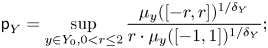 \begin{equation} {\mathsf{p}}_Y=\sup_{y\in Y_0, 0< r\le 2} \frac{\mu_{y}([-r,r])^{1/\delta_Y}}{r\cdot \mu_{y}([-1,1])^{1/\delta_Y}}; \end{equation}
the range  $0< r\leq 2$ is motivated by our applications later; see e.g. (7.13).
Recall the shadow constant  $\mathsf {s}_Y=\sup _{0<{\varepsilon }\le 1/2} \mathsf {s}_Y({\varepsilon })$ in (1.8) where
 \begin{equation} \mathsf{s}_Y({\varepsilon}):= \sup_{\xi\in \Lambda_Y, p\in [\xi,\Lambda_Y]} \frac{\nu_{p}(B_p(\xi,{\varepsilon}))^{1/\delta_Y}}{{\varepsilon}\cdot \nu_p(B_p(\xi, 1/2))^{1/\delta_Y}}, \end{equation}
where  $[\xi, \Lambda _Y]$ is the union of all geodesics connecting $\xi$ to a point in $\Lambda _Y$, and $B_p(\xi,\cdot )$ is as in (4.10).
The rest of this section is devoted to the proof of the following theorem using a uniform version of Sullivan's shadow lemma.
Theorem 4.8 We have
 \[ \mathsf{s}_Y\asymp \mathsf{p}_Y <\infty. \]
In principle, this definition of  $\mathsf {s}_Y$ involves making a choice of $\Delta _Y=\operatorname {Stab}_H(y_0)$, i.e. the choice of $y_0\in Y$, as $\Lambda _Y$ is the limit set of $\Delta _Y$. However, we observe the following.
Lemma 4.9 The constant  $\mathsf {s}_Y$ is independent of the choice of $y_0\in Y$.
Proof. Let  $y=y_0h^{-1}\in Y$ for $h\in H$. Define $\mathsf {s}'_Y$ similar to $\mathsf {s}_Y$ using $\Delta _Y'={\rm Stab}_H(y)=h\Delta _Yh^{-1}$ and put $\nu '_p:=h_*\nu _{h^{-1}p}$ for each $p\in \mathbb {H}^2$. If $\xi \in \Lambda _Y$, then
 \begin{align*} &\frac{d \bigl((h\gamma h^{-1})_* \nu_p'\bigr)}{d\nu_p'}(h\xi)=\frac{d \bigl((h\gamma)_* \nu_{h^{-1}p}\bigr)}{dh_*\nu_{h^{-1}p}}(h\xi) =\frac{d \gamma_* \nu_{h^{-1}p}}{d\nu_{h^{-1}p}}(\xi)\\ &\quad =e^{-\delta(Y) \beta_\xi(\gamma^{-1}(h^{-1}p), h^{-1}p)} =e^{-\delta(Y) \beta_{h\xi}(h\gamma^{-1}h^{-1}(p), p)}. \end{align*}
Since the limit set of  $\Delta '_Y$ is given by $h\Lambda _Y$, this implies that the family $\{\nu '_p: p\in \mathbb {H}^2\}$ is the Patterson–Sullivan density for $\Delta '_Y$. Now for any $0<{\varepsilon }\leq 1$ and $\xi \in \Lambda _Y$, we have
 \[ \nu_{hp}'(B_{hp}(h\xi,{\varepsilon}))=h_*\nu_{p}(B_{hp}(h\xi,{\varepsilon}))=\nu_{p}(h^{-1}B_{hp}(h\xi,{\varepsilon}))=\nu_p(B_p(\xi, {\varepsilon})). \]
It follows that  $\mathsf {s}_Y=\mathsf {s}'_Y$.
Shadow lemma
Consider the associated hyperbolic plane and its convex core:
 \[ S_Y:= \Delta_Y\backslash \mathbb{H}^2\quad \text{and}\quad {\operatorname{core}}\, (S_Y):=\Delta_Y\backslash \operatorname{hull}(\Lambda_Y). \]
We denote by  $C_Y$ the compact core of $S_Y$, defined as the minimal connected surface whose complement in $\operatorname {core}(S_Y)$ is a union of disjoint cusps. If $S_Y$ is convex cocompact, then $C_Y=S_Y$. Let
 \[ d_Y:=\max\{1, \operatorname{diam} (C_Y)\}. \]
We can write  ${\operatorname {core}}\,(S_Y)$ as the disjoint union of the compact core $C_0:=C_Y$ and finitely many cusps, say, $C_1, \ldots, C_m$. Fix a Dirichlet domain $\mathcal {F}_Y\subset \mathbb {H}^2$ for $\Delta _Y$ containing the base point $o$. For each $C_i$, $0\le i\le m$, choose the lift $\tilde {C}_i\subset \mathcal {F}_Y\cap \text {hull}(\Lambda _Y)$ so that $\Delta _Y\backslash \Delta _Y \tilde {C}_i=C_i$. In particular, $\partial \tilde {C}_0$ intersects $\tilde {C}_i$ in an interval for $i\ge 1$. Let $\xi _i\in \Lambda _Y$ be the base point of the horodisc $\tilde {C}_i$, i.e. $\xi _i=\partial \tilde {C}_i \cap \partial \mathbb {H}^2$. Let $F_{\xi _i}\subset \partial \mathbb {H}^2-\{\xi _i\}$ be a minimal closed interval so that $\Lambda _Y-\{\xi _i\}\subset \operatorname {Stab}_{\Delta _Y}(\xi _i) F_{\xi _i}$.
For  $p\in {}{\mathbb {H}}^2$, let $d_p$ denote the Gromov distance on $\partial \mathbb {H}^2$: for $\xi \ne \eta \in \partial \mathbb {H}^2$,
 \[ d_p(\xi, \eta)= e^{-(\beta_\xi(p,q) +\beta_\eta(p, q))/2} \]
where  $q$ is any point on the geodesic connecting $\xi$ and $\eta$. The diameter of $(\partial \mathbb {H}^2, d_p)$ is equal to $1$.
$1$.
For any  $h\in H$, we have $d_{p}(\xi, \eta )= d_{h(p)}(h(\xi ), h(\eta ))$. For $\xi \in \partial \mathbb {H}^2$, and $r>0$, set
 \begin{equation} B_p(\xi, r)=\{\eta\in \partial \mathbb{H}^2: d_p(\eta, \xi)\le r\} \end{equation}
as was defined in the introduction. Also, denote by  $V(p, \xi, r)$ the set of all $\eta \in \partial \mathbb {H}^2$ such that the distance between $p$ and the orthogonal projection of $\eta$ onto the geodesic $[p, \xi )$ is at least $r$. Note that
 \[ V(p, \xi, t )=B_p\bigg(\xi, \frac{e^{-t}}{\sqrt{1+e^{-2t}}}\bigg), \]
see ([Reference SchapiraSch04, Lemma 2.5] and the discussion following that lemma). Therefore,
 \[ V(p, \xi, r+1 )\subset B_p(\xi, e^{-r})\subset V(p,\xi, r-1)\quad \text{for all $r\ge 1$.} \]
The following is a uniform version of Sullivan's shadow lemma [Reference SullivanSul84]. The proof of this proposition is similar to the proof of [Reference SchapiraSch04, Theorem 3.2]; since the dependence on the multiplicative constant is important to us, we give a sketch of the proof while making the dependence of constants explicit.
Proposition 4.11 There exists a constant  $c\asymp e^{\star d_Y}$ such that for all $\xi \in \Lambda _Y$, $p\in \tilde {C}_0$, and $t>0$,
 \begin{align*} c^{-1}\cdot \nu_p(F_{{\xi}_t}) \beta_Y e^{-\delta(Y) t +(1-\delta(Y))d(\xi_t, \Delta_Y(p))} &\le \nu_p(V(p, \xi, t)) \\ &\le c \cdot \nu_p(F_{{\xi}_t}) e^{-\delta(Y) t +(1-\delta(Y))d(\xi_t, \Delta_Y(p))} \end{align*}
where:
•
$\{\xi _t\}$ is the unit speed geodesic ray $[p,\xi )$ so that $d(p, \xi _t)=t$;•
$F_{\xi _t}=\partial \mathbb {H}^2$ if $\xi _t\in \Delta _Y\tilde {C}_0$, and $F_{\xi _t}=F_{\xi _i}$ if $\xi _t\in \Delta _Y\tilde {C}_i$ for $1\le i\le m$;•
$\beta _Y:= \inf _{\eta \in \Lambda _Y, q\in \tilde {C}_0} \nu _q(B_q(\eta, e^{-d_Y}))$.


Proof. Let  $p$,
$p$,  $\xi \in \Lambda _Y$ and $\xi _t$ be as in the statement. By the $\delta (Y)$-conformality of the PS density, we have
 \[ \nu_p (V(p, \xi, t)) = e^{-\delta(Y) t} \nu_{\xi_t} (V(p, \xi, t)) . \]
Therefore it suffices to show
 \[ \nu_{\xi_t} (V(p, \xi, t)) \asymp \nu_p(F_{{\xi}_t})\cdot e^{(1-\delta(Y))d(\xi_t, \Delta_Y(p))} \]
while making the dependence of the implied constant explicit.
Claim A If  $\xi _t\in \Delta _Y \tilde {C}_0$, then
 \begin{equation} e^{-\delta(Y) d_Y} \cdot \inf_{\eta\in \Lambda_Y} \nu_p(B(\eta, e^{-d_Y}))\ll \nu_{\xi_t} (V(p, \xi, t)) \ll e^{\delta(Y) d_Y} |\nu_p| \end{equation}
where the implied constants are absolute.
First note that this implies the claim in the proposition if  $\xi _t\in \Delta _Y \tilde {C}_0$. Indeed $d(\xi _t, \Delta _Y(p))\leq d_Y$ and $F_{\xi _t}=\partial \mathbb {H}^2$ in this case. Moreover, by (4.12), we have
 \[ e^{-\star d_Y}\beta_Y e^{-\delta(Y) t}\leq \nu_p (V(p, \xi, t)) = e^{-\delta(Y) t} \nu_{\xi_t} (V(p, \xi, t)) \leq e^{\star d_Y} e^{-\delta(Y) t} \]
where we also used  $|\nu _p|=e^{\star d_Y}$ (recall that $p\in \tilde {C}_0$). Thus the claim in the proposition follows in this case.
We now turn to the proof of Claim A. As  $\xi _t\in \Delta _Y \tilde {C}_0$, there exists $\gamma \in \Delta _Y$ such that ${d(\xi _t, \gamma p) \le d_Y}$. Hence
 \begin{align*} e^{-\delta(Y) d_Y} \nu_{\xi_t} (V(p, \xi, t)) &\le \nu_{\gamma p} (V(p, \xi, t))= \nu_p (V(\gamma^{-1}p, \gamma^{-1}\xi, t))\\ &\le e^{{\delta(Y)} d_Y} \nu_{\xi_t} (V(p, \xi, t)). \end{align*}
The upper bound in (4.12) follows from the first inequality, while the lower bound follows from the second inequality; indeed
 \[ V(\gamma^{-1}p, \gamma^{-1}\xi, t)=V(\gamma^{-1}\xi_t, \gamma^{-1}\xi, 0) \]
and the latter contains  $B_p(\gamma ^{-1} \xi, e^{-d_Y})$, since $d(p, \gamma ^{-1}\xi _t)\le d_Y$ and $d_Y\geq 1$.
Claim B Let  $\xi$ be a parabolic limit point in $\Lambda _Y$. Assume that for some $i\ge 1$, $\xi _t\in \tilde {C}_i$ for all large $t$.
$t$.
We claim
 \begin{equation} \nu_{\xi_t} (V(p, \xi, t))\asymp \nu_p(F_\xi) \cdot e^{(1-\delta(Y))(d(\xi_t, \Delta_Y(p)) +d_Y)} \end{equation}
and
 \begin{equation} \nu_{\xi_t} (\partial \mathbb{H}^2-V(p, \xi, t))\asymp \nu_p(F_\xi) \cdot e^{(1-\delta(Y))(d(\xi_t, \Delta_Y(p)) +d_Y)} \end{equation}
where here and in what follows implied constants are of the form  $e^{\pm \star d_Y}$ unless otherwise is stated explicitly.
Let  $s_i\ge 0$ be such that $\xi _{s_i}\in \partial \tilde {C}_i$. Then for all $t\ge s_i$,
 \[ |d(\xi_t, \Delta_Y(p)) -(t-s_i)|\le d_Y. \]
Hence for (4.13), it suffices to show
 \begin{equation} \nu_{\xi_t} (V(p, \xi, t))\asymp e^{(1-\delta(Y))(t-s_i)}\nu_p(F_\xi). \end{equation}
Note that if we set  $\Delta _{Y,\xi }=\operatorname {Stab}_{\Delta _Y}(\xi )$,
 \[ \nu_{\xi_t} (V(p, \xi, t)) \asymp \sum_{\gamma \in \Delta_{Y, \xi}, \gamma F_\xi \cap V(p, \tilde{x}, t)\ne \emptyset} \nu_{\xi_t}(\gamma F_\xi) . \]
Let  $F^*_{\xi }$ denote the image of $F_\xi$ on the horocycle based at $\xi$ passing through $p$ via the inverse of the visual map. Since $p\in \tilde {C}_0$, there exists $\gamma \in \Delta _{Y, \xi }$ so that $\gamma F^*_{\xi }$ is contained in the closure of $\tilde {C}_0$. Hence,
 \[ \text{diam}\,F^*_{\xi}\le d_Y=\max\{1,\text{diam}(\tilde{C}_0)\}. \]
We now apply [Reference SchapiraSch04, Lemma 2.9] with  $K=F^*_{\xi }$ and let $K_3$ be as in [Reference SchapiraSch04]. By the definition of $K_3$ given in the proof of [Reference SchapiraSch04, Lemma 2.9], we have $K_3\ll \text {diam}\,F^*_{\xi }$ where the implied constant is absolute. Thus, in view of [Reference SchapiraSch04, Lemma 2.9], if $\gamma \in \Delta _{Y, \xi }$ is so that $\gamma F_\xi \cap V(p, \xi, t)\ne \emptyset$, then $d(p, \gamma p)\ge 2t -kd_Y$, where $k$ is absolute. In consequence,
 \[ \nu_{\xi_t} (V(p, \xi, t)) \asymp \sum_{\gamma \in \Delta_{Y, \xi}, d(p, \gamma p)\ge 2t} \nu_{\xi_t}(\gamma F_\xi) \]
where the implied constant is absolute.
Now we use the fact that if  $d(p, \gamma p)\ge 2t$, then for all $\eta \in F_\xi$,
 \[ |\beta_\eta (\gamma^{-1}\xi_t, \xi_t) -d(p, \gamma p) +2t|\ll \text{diam}\,F^*_{\xi}\le d_Y \]
(cf. proof of [Reference SchapiraSch04, Lemma 2.9]). Since
 \[ \nu_{\xi_t}(\gamma F_\xi)=\int_{\gamma F_\xi}\,d\nu_{\xi_t}=\int_{F_\xi} e^{-\delta(Y) \beta_{\gamma\eta}(\xi_t, \gamma \xi_t))}\,d\nu_{\xi_t}(\eta), \]
and  $\nu _{\xi _t}(F_\xi )= e^{-\delta (Y) t}\nu _p(F_\xi )$, we deduce, with multiplicative constant $\asymp e^{\delta (Y) d_Y}$,
 \begin{align*} \sum_{\gamma \in \Delta_{Y, \xi}, d(p, \gamma p)\ge 2t} \nu_{\xi_t}(\gamma F_\xi) &\asymp \sum_{\gamma \in \Delta_{Y, \xi}, d(p, \gamma p)\ge 2t} e^{2\delta(Y) t -\delta(Y) d(p, \gamma p) } \nu_{\xi_t}(F_\xi) \\ &\asymp \nu_p(F_\xi) e^{\delta(Y) t }\sum_{\gamma \in \Delta_{Y, \xi}, d(p, \gamma p)\ge 2t} e^{-\delta(Y) d(p, \gamma p)}\\ & \asymp \nu_p(F_\xi) e^{(1-\delta(Y)) t } \end{align*}
using  $a_n:=\#\{\gamma \in \Delta _{Y, \xi }: n< d(p, \gamma p)\le n+1\} \asymp e^{n/2}$ in the last estimate. This proves (4.13).
The estimate (4.14) follows similarly now using
 \[ \nu_{\xi_t} (\partial \mathbb{H}^2-V(p, \xi, t)) \asymp \sum_{\gamma \in \Delta_{Y, \xi}, d(p, \gamma p)\le 2t} \nu_{\xi_t}(\gamma F) \]
and  $\sum _{n=0}^{[2t]} a_n e^{-\delta (Y) n} \asymp e^{(1-2\delta (Y) )t}$.
Note that when  $\xi$ is a parabolic limit point, (4.13) holds with multiplicative constant $\asymp e^{\star d_Y}$ (see the proof of [Reference SchapiraSch04, Proposition 3.4]).
As for the remaining case, i.e.  $\xi$ is a radial limit point but $\xi _t\in \Delta _Y \tilde {C}_i$ for some $i$, one can prove that (4.13) holds with multiplicative constant $\asymp e^{\star d_Y}$ (see the proof of [Reference SchapiraSch04, Lemma 3.6]).
Proposition 4.16 Fix  $p=p_Y\in \tilde {C}_0$. There exists $R_Y\asymp e^{\star d_Y}$ such that for all $y\in Y_0$, we have
 \[ {R_Y^{-1}}{\beta_Y } e^{(1-\delta(Y))d(C_Y, \pi(y))} |\nu_p| \leq {\mu_y([-1,1])} \leq R_Y e^{(1-\delta(Y)) d(C_Y, \pi(y))} |\nu_p| \]
where  $\pi$ denotes the base point projection $\Delta _Y\backslash H =\operatorname {T}^1(S_Y) \to S_Y$.
Proof. The following argument is a slight modification of the proof of [Reference Maucourant and SchapiraMS14, Proposition 5.1]. Since the map  $y\mapsto \mu _y[-1,1]$ is continuous on $Y_0$ and $\{[h]\in Y_0: h^-\text { is a radial limit point of }\Lambda _Y\}$ is dense in $Y_0$, it suffices to prove the claim for $y=[h]$, assuming that $h^-$ is a radial limit point for $\Delta _Y$.
Recall that  ${\mu _y([-1,1])}=e^{\delta (Y) t} {\mu _{ya_{-t}}([-e^{-t}, e^{-t}])}$ for all $t\in \mathbb {R}$. Let $t\ge 0$ be the minimal number so that $\pi (ya_{-t})\in C_Y$; this exists as $h^-$ is a radial limit point. Then
 \begin{equation} d(\pi(y), C_Y)\leq d(\pi(y), \pi(ya_{-t}))\leq d_Y + d(\pi(y), C_Y). \end{equation}
 Set  $\xi _t=ha_{-t}(o)$. Then
 \[ \mu_{ya_{-t}} [-e^{-t}, e^{-t}]\asymp \nu_{\xi_t}(V(\xi_t, h^+, {t})) \]
(cf. [Reference SchapiraSch04, Lemma 4.4]).
Since  $ya_{-t}\in C_Y$, $F_{\xi _t}=\partial \mathbb {H}^2$. So $\nu _{\xi _t} (F_{\xi _t} )=|\nu _{\xi _t}|\asymp |\nu _p|$ up to a multiplicative constant $e^{\star d_Y}$. Therefore, for some implied constant $\asymp e^{\star d_Y}$, we have
 \begin{align*} \beta_Y e^{-\delta(Y) t +(1-\delta(Y))d(\pi(y), \pi(ya_{-t}))} |\nu_p| &\ll \nu_{\xi_t}(V(\xi_t, h^+, t)) \\ &\ll e^{-\delta(Y) t +(1-\delta(Y))d(\pi(y), \pi(ya_{-t}))} |\nu_p|. \end{align*}
This estimate and (4.17), therefore, imply that
 \[ \beta_Y e^{(1-\delta(Y))d(\pi(y), C_Y)} |\nu_p| \ll \mu_y([-1,1]) \ll e^{(1-\delta(Y))d(\pi(y), C_Y)} |\nu_p| \]
with the implied constant  $\asymp e^{\star d_Y}$, proving the claim.
We use the following result, essentially obtained by Schapira and Maucourant [Reference SullivanSul84, Reference Maucourant and SchapiraMS14].
Corollary 4.18 Fix  $\rho >0$. Then for all $0<{\varepsilon }\leq \rho$,
 \[ {R_Y^{-2}\cdot \beta_Y}\le \sup_{y\in Y_0} \frac{\mu_{y}([-{\varepsilon},{\varepsilon}])}{{\varepsilon}^{\delta_Y}\mu_{y}([-1,1])}\le \max\{1,\rho^2\}\cdot R_Y^2\cdot {\beta_Y^{-1}} <\infty, \]
where  $R_Y$ is as in Proposition 4.16.
Proof. By (4.3), we have  $\mu _y([-{\varepsilon },{\varepsilon }])={\varepsilon }^{\delta (Y)} \mu _{ya_{-\log {\varepsilon }}}([-1,1]).$ Hence the case when $Y$ is convex cocompact follows from Proposition 4.16.
Now suppose that  $Y$ has a cusp. Let $y\in Y_0$. Using the triangle inequality, we get that $d(\pi (ya_{-\log {\varepsilon }}), C_Y)-d(\pi (y), C_Y) \le |\log {\varepsilon }|$. Therefore, by Proposition 4.16, we have
 \begin{align*} \frac{\mu_{ya_{-\log {\varepsilon}}}([-1,1])}{\mu_y([-1,1])} &\le R_Y^2 \beta_Y^{-1} \cdot e^{(1-\delta(Y)) (d(\pi(y a_{-\log {\varepsilon}}), C_Y)-d(\pi(y), C_Y) ) }\\ &\le \begin{cases} R_Y^2 \cdot\beta_Y^{-1}\cdot {\varepsilon}^{\delta(Y)-1} & \text{if $0<{\varepsilon} <1$,}\\ R_Y^2 \cdot\beta_Y^{-1}\cdot{\varepsilon}^{1-\delta(Y)} & \text{if ${\varepsilon}\geq 1$.}\end{cases} \end{align*}
As a consequence, we have
 \[ \frac{\mu_y([-{\varepsilon},{\varepsilon}])}{{\varepsilon}^{2\delta(Y)-1} \mu_y([-1,1])} \le \begin{cases} R_Y^2 \cdot\beta_Y^{-1} & \text{if $0<{\varepsilon} <1$,}\\ R_Y^2 \cdot\beta_Y^{-1}\cdot\rho^2 & \text{if $\rho\geq 1$ and $1\leq {\varepsilon}\leq \rho$.}\end{cases} \]
Recall from (4.5) that  $\delta _Y=\delta (Y)$ when $Y$ is cocompact and $\delta _Y=2\delta (Y)-1$ otherwise. The above thus establishes the upper bound.
By choosing  $y\in Y_0$ such that $d(\pi (ya_{-\log {\varepsilon }}), C_Y)-d(\pi (y), C_Y) =|\log {\varepsilon }|$, we get the lower bound.
Theorem 4.8 follows from the following proposition.
Proposition 4.19 We have:
(1) for any
$0<{\varepsilon }\le 1/2$, $0<\mathsf {s}_Y({\varepsilon })<\infty$;(2)
$\mathsf {s}_Y\asymp {\mathsf {p}}_Y \ll {e^{\star d_Y/\delta _Y} } \beta _Y^{-1/\delta _Y}$.


Proof. Let  $y\in Y_0$ and $h\in H$ be so that $y=[h]$. Fix $0< r\le 2$. Recall
 \[ \mu_y([-r,r])=\int_{-r}^r e^{-\delta(Y)\beta_{hu_s^+} (h(o), hu_s(o)) }\,d\nu_{h(o)} (hu_s^+). \]
Since  $|\beta _{hu_r^+} (h(o), hu_r(o))|\le d(o, u_r(o))$, we have
 \[ e^{-\delta(Y)\beta_{hu_r^+} (h(o), hu_r(o)) }\asymp 1 \]
with the implied constant independent of all  $0< r\le 2$.
Since  $d_o(u_r^+, e^+)= d_{h(o)} ((hu_r)^+, h^+)$ where $e$ is the identity (recall that $v_o^+=e^+$), we have
 \[ \nu_{h(o)}\bigg(B_{h(o)}\bigg(h^+, \frac{c^{-1} r}{\sqrt{1+2r^2}}\bigg)\bigg) \ll \mu_y([-r,r]) \ll \nu_{h(o)}\bigg(B_{h(o)}\bigg(h^+, \frac{c r}{\sqrt{1+2r^2}}\bigg)\bigg) \]
for some  $c>1$ independent of $r$ and $h$.
$h$.
This implies that
 \[ \mu_y([{-{\varepsilon}}/{c'} , {{\varepsilon}}/{c'}] ) \ll \nu_{h(o)}(B_{h(o)}(h^+, {\varepsilon}))\ll \mu_y([{-c'{\varepsilon}}, {c' {\varepsilon}}]) \]
as well as
 \[ \frac{\mu_y([{-{\varepsilon}}/{c'} , {{\varepsilon}}/{c'}] )}{{\varepsilon}^{\delta_Y}\mu_y([{-c'}/{2},{c'}/{2}])}\ll\frac{\nu_{h(o)}(B_{h(o)}(h^+, {\varepsilon}))}{{\varepsilon}^{\delta_Y}\nu_{h(o)}(B_{h(o)}(h^+, 1/2))}\ll \frac{\mu_y([{-c'{\varepsilon}}, {c' {\varepsilon}}]) }{{\varepsilon}^{\delta_Y}\mu_y([{-1}/({2c'}),{1}/({2c'})])} \]
where  $c'>1$ is independent of $0<{\varepsilon }<1/2$ and $h\in H$.
First note that by Corollary 4.18, we have
 \[ \mu_y([{-1}/({2c'}),{1}/({2c'})])\asymp_{c'}\mu_{y}[-1,1]\asymp_{c'}\mu_y([{-c'}/{2},{c'}/{2}]) . \]
Similarly, using Corollary 4.18, for any  $0<{\varepsilon }\leq 1/2$, we have
 \[ \mu_y([{-{\varepsilon}}/{c'} , {{\varepsilon}}/{c'}])\asymp_{c'}\mu_{y}[-4{\varepsilon},4{\varepsilon}]\asymp_{c'}\mu_y([-c'{\varepsilon},c'{\varepsilon}]); \]
the choice of the constant  $4$ here is motivated by the definitions of $\mathsf {p}_Y$ and $\mathsf {s}_Y$ in (4.6) and (4.7), respectively.
Altogether we conclude that
 \[ \frac{\nu_{h(o)}(B_{h(o)}(h^+, {\varepsilon}))}{{\varepsilon}^{\delta_Y}\nu_{h(o)}(B_{h(o)}(h^+, 1/2))}\asymp \frac{\mu_y([-4{\varepsilon}, 4{\varepsilon}]) }{(4{\varepsilon})^{\delta_Y}\mu_y([-1,1])}. \]
Taking supremum over  $0<{\varepsilon }\leq 1/2$ and $h\in H$ with $h^\pm \in \Lambda _Y$, we conclude that $\mathsf {s}_Y\asymp \mathsf {p}_Y$.
The last claim follows from Corollary 4.18.
5. Linear algebra lemma
The goal of this section is to prove the linear algebra lemma (Lemma 5.6) and its slight variant (Lemma 5.13).
In this section, it is more convenient to identify  $G$ as $\operatorname {SO}(\mathsf {Q})^\circ$ for the quadratic form
 \[ \mathsf{Q}(x_1,x_2,x_3,x_4)=2x_1x_4-x_2^2-x_3^2. \]
As  $\mathsf {Q}$ has signature $(1,3)$, $\operatorname {PSL}_2(\mathbb {C})\simeq \operatorname {SO}(\mathsf {Q})^\circ$ as real Lie groups. We consider the standard representation of $G$ on the space $\mathbb {R}^4$ of row vectors and denote the Euclidean norm on $\mathbb {R}^4$ by $\|\cdot \|$. We have
 \[ H=\operatorname{Stab}_G(e_3)\simeq \operatorname{SO}(1,2)^\circ, \]
 \[ A=\{a_t=\text{diag}(e^t, 1,1, e^{-t}):t\in \mathbb{R}\}< H, \]
 \[ U=\left\{u_r=\begin{pmatrix}1 & 0 & 0 & 0\\ r & 1 & 0 & 0\\ 0 & 0 & 1 & 0 \\ {r^2}/{2} & r & 0 & 1\end{pmatrix}: r\in\mathbb{R}\right\}< H. \]
Set
 \[ V:=\mathbb{R} e_1\oplus \mathbb{R} e_2\oplus\mathbb{R} e_4. \]
Then the restriction of the standard representation of  $G$ to $H$ induces a representation of $H$ on $V$, which is isomorphic to the adjoint representation of $H$ on its Lie algebra $\mathfrak {sl}_2(\mathbb {R})$; in particular, it is irreducible.
Note that for each  $t>0$, $\mathbb {R} e_2=\{v\in V: va_t=v\}$, $\mathbb {R} e_1$ is the subspace of all vectors with eigenvalues $>1$, and $\mathbb {R}e_4$ is the subspace of all vectors with eigenvalues $<1$.
$<1$.
Let  $p:V\to \mathbb {R}e_1\oplus \mathbb {R}e_2$ and $p^+: V\to \mathbb {R}e_1$ denote the natural projections. Writing $v=v_1e_1+v_2e_2+v_4e_4$, a direct computation yields that for any $r\in \mathbb {R}$,
 \begin{equation} p(vu_r)=\bigg(v_1+v_2r+\frac{v_4r^2}{2} \bigg)e_1+ (v_2+v_4r)e_2\quad\text{and}\quad p^+(vu_r)=\bigg(v_1+v_2r+\frac{v_4r^2}{2}\bigg)e_1. \end{equation}
 For a unit vector  $v\in V$ and ${\varepsilon }>0$, define
 \begin{align} D(v,{\varepsilon})&=\{r\in[-1,1]: \|p(vu_{r})\| \le {\varepsilon}\},\nonumber \end{align}
 \begin{align} D^+(v,{\varepsilon})&=\{r\in[-1,1]: \|p^+(vu_{r})\| \le {\varepsilon}\}.\nonumber \end{align}
Lemma 5.2 For all  $0<{\varepsilon }<1/2$ and a unit vector $v\in V$, we have
 \[ \ell (D(v,{\varepsilon})) \ll {\varepsilon}\quad\text{and}\quad \ell (D^+(v,{\varepsilon})) \ll {\varepsilon}^{1/2} \]
where  $\ell$ denotes the Lebesgue measure on $\mathbb {R}$.
Proof. Since we are allowed to choose the implied constant in the statement, it suffices to prove the lemma for  $0<{\varepsilon }\leq 0.01$.
Writing  $v=v_1e_1+v_2e_2+v_4e_4$, we have
 \[ \ell (D(v,{\varepsilon}))\le \ell \bigg\{r\in[-1,1]: \bigg|v_1+v_2r+ \frac{v_4r^2}2\bigg|\leq {\varepsilon}\text{ and }|v_2+v_4r|\leq {\varepsilon}\bigg\}. \]
If  $|v_4|\geq 0.01$, then
 \[ \ell (D(v,{\varepsilon})) \le \ell \{r\in[-1,1]: |v_2+v_4r|\leq {\varepsilon}\}\le 200 {\varepsilon}. \]
If  $|v_4|< 0.01$ but $0.1\leq |v_2|\leq 1$, then for $r\in [-1,1]$, we have $|v_2+v_4r|\ge 0.09$, and hence for all ${\varepsilon }\leq 0.01$,
 \[ \ell (D(v,{\varepsilon})) \le \ell \{r\in[-1,1]: |v_2+v_4r|\leq {\varepsilon}\}=0. \]
Now consider the case when  $|v_4|\leq 0.01$ and $|v_2|\leq 0.1$. Then, since $\|v\|=1$, we get that $|v_1|\geq 0.7$. Hence for all $r\in [-1,1]$, $|v_1+v_2r+v_4r^2/2|> 0.5$. In consequence, for all ${\varepsilon }<1/2$,
 \[ \ell (D(v, {\varepsilon}))\le \ell \{r\in[-1,1]: |v_1+v_2r+v_4r^2/2|\leq {\varepsilon}\}= 0, \]
proving the estimate on  $D(v,{\varepsilon })$. To estimate $D^+(v,{\varepsilon })$, observe that $p^+(vu_{r})=(v_1+v_2r+ {v_4r^2}/{2})e_1$ is a polynomial map of degree at most $2$. Moreover, since $\|v\|=1$, we have
 \[ \max\{|v_1|, |v_2|, |v_4|\}\gg1. \]
Therefore,  $\sup _{{r}\in [-1,1]}\|p^+(vu_{r})\|\gg 1$. The claim about $D^+(v,{\varepsilon })$ now follows using Lagrange's interpolation; see [Reference Brudnyi and GanzburgBG73] for a more general statement.
For the rest of this section, we fix a closed non-elementary  $H$-orbit $Y$.
$Y$.
Lemma 5.3 There exists an absolute constant  $\hat b_0>0$ for which the following holds: for any $y\in Y_0$ and $0<{\varepsilon } <1$, we have
 \begin{equation} \sup_{ v\in V,\|v\|=1}\mu_{y}{}(D(v,{\varepsilon}))\leq \hat b_0 {\mathsf{p}}_Y^{\delta_Y} {\varepsilon}^{\delta_Y} \mu_y([-1,1]), \end{equation}
and
 \begin{equation} \sup_{ v\in V,\|v\|=1} \mu_{y}{}(D^+(v,{\varepsilon}))\leq \hat b_0 {\mathsf{p}}_Y^{\delta_Y} {\varepsilon}^{{\delta_Y/}{2}} \mu_y([-1,1]) \end{equation}
where  ${\mathsf {p}}_Y$ is given as in (4.6).
Proof. By (5.1), each set  $D(v,{\varepsilon })$ and $D^+(v,{\varepsilon })$ consists of at most two intervals. By Lemma 5.2, $D(v,{\varepsilon })$ (respectively $D^+(v,{\varepsilon })$) may be covered by $\ll 1$ many intervals of length ${\varepsilon }$ (respectively ${\varepsilon }^{1/2}$). Therefore (5.4) (respectively (5.5)) follows from the definition of ${\mathsf {p}}_Y$.
We use Lemma 5.3 to prove the following lemma which will be crucial in what follows.
Lemma 5.6 (Linear algebra lemma)
For any  $ {\delta _Y}/{3}\le s < {\delta _Y}$, $1\le \rho \le 2$, and $t>0$, we have
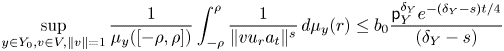 \begin{equation} \sup_{y\in Y_0, v\in V, \|v\|=1} \frac{1}{ \mu_y([-\rho,\rho])}\int_{-\rho}^{\rho} \frac{1}{\| vu_r a_t\|^s} \,d\mu_{y}{} (r) \le b_0 \frac{{\mathsf{p}}_Y^{\delta_Y} e^{-(\delta_Y- s)t/4} }{(\delta_Y-s)} \end{equation}
where  $b_0\ge 2$ is an absolute constant.
Proof. We first claim that it suffices to prove the claim for  $\rho =1$. Indeed, let $t_\rho =t-\log \rho$ and let $y_\rho =ya_{-\log \rho }$, and for every $v\in V$, let $v_\rho =va_{-\log \rho }$. Recall also that $\mu _y[-r,r]=\rho ^{\delta (Y)} \mu _{ya_{-\log \rho }}{} [-r/\rho,r/\rho ]$ and that $Y_0$ is $A$-invariant. Thus,
 \begin{align*} \frac{1}{ \mu_y([-\rho,\rho])}\int_{-\rho}^{\rho} \frac{1}{\| vu_r a_t\|^s} \,d\mu_{y}(r)&=\frac{1}{ \mu_y([-\rho,\rho])}\int_{-\rho}^{\rho}\frac{1}{\| va_{-\log\rho}u_{\rho^{-1}r} a_{t_\rho}\|^s} \,d\mu_{y}(r) \\ &=\rho^{\delta(Y)}\|v_\rho\|^{-s}\frac{1}{ \mu_{y_\rho}([-1,1])}\int_{-1}^{1}\frac{1}{\| v_\rho' u_{r} a_{t_\rho}\|^s}\,d\mu_{y_\rho}(r) \end{align*}
where  $v'_\rho =v_\rho /\|v_\rho \|$.
Since  $\|v_\rho \|^{-s}\asymp 1$ (with absolute implied constants for $1\leq \rho \leq 2$) and $Y_0$ is $A$-invariant, it thus suffices to prove the lemma for $\rho =1$.
Fix  $0< s<\delta _Y$ and $t>0$. We observe that for all $r\in \mathbb {R}$,
 \begin{equation} \text{$\|vu_ra_t\|\geq \|p(vu_r)\|\quad$ and $\quad\| v u_{r} a_t\| \ge e^{t} \|p^+(vu_{r})\|$.} \end{equation}
 For simplicity, set  $\beta _y:= {1}/{\mu _{y}{}([-1,1])}$. The inequality (5.4) and the first estimate in (5.8) imply that for any $0<{\varepsilon }\leq 1$ and any unit vector $v\in V$, we have
 \begin{align*} \beta_y \int_{{r}\in D(v,{\varepsilon} )- D(v, {\varepsilon} /2)} {\| vu_{r}a_t\|^{-s}} d\mu_{y}{}({r}) &\le {\hat b_0 {\mathsf{p}}_Y}^{\delta_Y} {\varepsilon}^{\delta_Y} \cdot ({\varepsilon}/2)^{-s} \\ &\le 2\hat b_0 {\mathsf{p}}_Y^{\delta_Y} {\varepsilon}^{\delta_Y-s}. \end{align*}
We write  $D(v,{\varepsilon })=\bigcup _{k=0}^\infty D(v, {\varepsilon }/2^k) -D(v, {\varepsilon }/2^{k+1})$. Now applying the above estimate for each ${\varepsilon }/2^k$ and summing up the geometric series, we get that for any $0<{\varepsilon }<1$,
 \begin{equation} \beta_y \int_{{r}\in D(v, {\varepsilon})} {\| vu_{r}a_t\|^{-s}} \,d\mu_{y}{}({r}) \le \frac{2\hat b_0 {\mathsf{p}}_Y^{\delta_Y} {\varepsilon}^{\delta_Y-s}}{1 -2^{s-\delta_Y}} . \end{equation}
 Moreover, using (5.5) and the first estimate in (5.8) again, for any  $\kappa >0$, we have
 \begin{equation} \beta_y \int_{{r}\in D^+(v,\kappa)- D(v, {\varepsilon})} {\| vu_{r}a_t\|^{-s}} \,d\mu_{y}{}({r})\leq~2\hat b_0 {\mathsf{p}}_Y^{\delta_Y}\kappa^{\delta_Y/2}{\varepsilon}^{-s}. \end{equation}
Finally, the definition of  $D^+(v, \kappa )$ and the second estimate in (5.8) imply
 \begin{equation} \beta_y \int_{{r}\in [-1,1]-D^+(v,\kappa)} {\| vu_{r}a_t\|^{-s}} \,d\mu_{y}{}({r})\leq \kappa^{-s} e^{-st}. \end{equation}
Combining (5.9), (5.10), and (5.11) and using the inequality  ${1}/({1-2^{-(\delta _Y-s)}}) \le {2}/({\delta _Y-s})$, we deduce that for any $0<{\varepsilon }, \kappa <1$,
 \[ \beta_y \int_{-1}^1 {\| vu_{r}a_t\|^{-s}} \,d\mu_{y}{}({r})\le \frac{2\hat b_0\mathsf{p}_Y^{\delta_Y} }{\delta_Y-s} \big({\varepsilon}^{\delta_Y-s} +\kappa^{\delta_Y/2} {\varepsilon}^{-s} +\kappa^{-s} e^{-st}\big). \]
Let  $\varepsilon =e^{-t/4}$ and $\kappa ={\varepsilon }^{2}$. As $\delta _Y/3 \le s<\delta _Y$, we have $e^{-s/2}\le e^{(s-\delta _Y)/4}$. This yields
 \[ \beta_y \int_{-1}^1 {\| vu_{r}a_t\|^{-s}} \,d\mu_{y}{}({r})\leq \frac{6\hat{b}_0\mathsf{p}_Y^{\delta_Y} }{\delta_Y-s} \cdot e^{-(\delta_Y-s)t/4}, \]
as we claimed.
We will extend the upper bound in Lemma 5.6 to all unit vectors  $v\in e_1G$, based on the fact that the vectors in $e_1G$ are projectively away from the $H$-invariant point corresponding to $\mathbb {R} e_3$.
Lemma 5.12 There exists an absolute constant  $b_1>1$ such that for any vector $v\in e_1G\subset \mathbb {R}^4$,
 \[ \|v\| \le b_1 \|v_1\| \]
where  $v_1$ is the projection of $v\in \mathbb {R}^4$ to $V=\mathbb {R} e_1\oplus \mathbb {R} e_2\oplus \mathbb {R} e_4$.
Proof. Since  $\mathsf {Q}(e_1)=0$ and $G=\operatorname {SO}(\mathsf {Q})^\circ$, we have $\mathsf {Q}(e_1g)=0$ for every $g\in G$. Since $\mathsf {Q}(e_3)=-1$, the set $\{\|v\|^{-1} v: v\in e_1G\}$ is a compact subset of the unit sphere in $\mathbb {R}^4$ not containing $\pm e_3$. Therefore there exists an absolute constant $0<\eta <1$ such that if we write $v=v_1 +re_3\in e_1G$, then $|r|\le \eta \|v\|$. Therefore $\|v_1\|^2=\|v\|^2 -r^2 \ge (1-\eta ^2)\|v\|^2$. Hence it suffices to set $b_1=(1-\eta ^2)^{-1/2}$.
Lemma 5.13 (Linear algebra lemma II)
For any  $ {\delta _Y}/{3}\le s < {\delta _Y}$, $1\le \rho \le 2$, and $t>0$, we have
 \[ \sup_{y\in Y_0,v\in e_1G, \|v\|=1} \frac{1}{ \mu_y([-\rho,\rho])}\int_{-\rho}^{\rho} \frac{1}{\| vu_r a_t\|^s} \,d\mu_{y}{} (r) \le b_0 b_1\frac{{\mathsf{p}}_Y^{\delta_Y} e^{-(\delta_Y- s)t/4} }{(\delta_Y-s)} \]
where  $b_0\ge 2$ and $b_1>1$ are absolute constants as in Lemmas 5.6 and 5.12 respectively.
Proof. Let  $v\in e_1G$ be a unit vector, and write $v=v_0+v_1$ where $v_0\in \mathbb {R} e_3$ and $v_1\in V$. Since $e_3$ is $H$-invariant, we have $vh=v_0+v_1h\in \mathbb {R} e_3\oplus V$ for all $h\in H$. Therefore,
 \begin{align*}
\frac{1}{\mu_y([-\rho,\rho])}\int_{-\rho}^{\rho}
\frac{1}{\| vu_r a_t\|^s} \,d\mu_y(r)&\leq
\frac{1}{\mu_y([-\rho,\rho])}\int_{-\rho}^{\rho}
\frac{1}{\| v_1u_r a_t\|^s} \,d\mu_y(r)\\ & \le
\frac{b_0{\mathsf{p}}_Y^{\delta_Y} e^{-(\delta_Y-s)t/4}
}{(\delta_Y-s)} \|v_1\|^{-s}\quad \text{by Lemma }\mbox{5.6}\\ &\le \frac{
b_0b_1{\mathsf{p}}_Y^{\delta_Y} e^{-(\delta_Y- s)t/4}
}{(\delta_Y-s)} \|v\|^{-s}\quad\text{by Lemma }\mbox{5.12}.
\end{align*}
\begin{align*}
\frac{1}{\mu_y([-\rho,\rho])}\int_{-\rho}^{\rho}
\frac{1}{\| vu_r a_t\|^s} \,d\mu_y(r)&\leq
\frac{1}{\mu_y([-\rho,\rho])}\int_{-\rho}^{\rho}
\frac{1}{\| v_1u_r a_t\|^s} \,d\mu_y(r)\\ & \le
\frac{b_0{\mathsf{p}}_Y^{\delta_Y} e^{-(\delta_Y-s)t/4}
}{(\delta_Y-s)} \|v_1\|^{-s}\quad \text{by Lemma }\mbox{5.6}\\ &\le \frac{
b_0b_1{\mathsf{p}}_Y^{\delta_Y} e^{-(\delta_Y- s)t/4}
}{(\delta_Y-s)} \|v\|^{-s}\quad\text{by Lemma }\mbox{5.12}.
\end{align*}
6. Height function $\omega$

In this section we define the height function  $\omega :X_0\to (0, \infty )$ and show that $\omega (x)$ is comparable to the reciprocal of the injectivity radius at $x$.
$x$.
For this purpose, we continue to realize  $G$ as $\operatorname {SO}(\mathsf {Q})^\circ$ acting on $\mathbb {R}^4$ by the standard representation, as in § 5. Observe that $\mathsf {Q}(e_1)=0$ and the stabilizer of $e_1$ in $G$ is equal to $M_0N$.
Fixing a set of  $\Gamma$-representatives $\xi _1, \ldots, \xi _\ell$ in $\Lambda _{\rm bp}$, choose elements $g_i\in G$ so that $g_i^-=\xi _i$ and $\|e_1g_i^{-1}\|=1$; this is possible since $\{g\in G: g^-=\xi _i\}$ is a conjugate of $AM_0N$.
Set
 \begin{equation} v_i:= e_1g_i^{-1}\in e_1G.\end{equation}
Note that
 \[ {\rm Stab}_G(\xi_i)=g_i A M_0 Ng_i^{-1}\quad\text{and}\quad \operatorname{Stab}_G(v_i)= g_iM_0 Ng_i^{-1} . \]
By Witt's theorem, we have that for each  $i$,
$i$,
 \begin{align*} \{v\in \mathbb{R}^4-\{0\}: \mathsf{Q}(v)=0\}=v_iG\simeq g_iM_0 Ng_i^{-1}\backslash G. \end{align*}
Lemma 6.2 For each  $1\le i\le \ell$, the orbit $v_i\Gamma$ is a closed (and hence discrete) subset of $\mathbb {R}^4$.
Proof. The condition  $\xi _i\in \Lambda _{\rm bp}$ implies that $\Gamma \backslash \Gamma g_i M_0N$ is a closed subset of $X$. Equivalently, $\Gamma g_i M_0N$ as well as $\Gamma g_i M_0N g_i^{-1}$ is closed in $G$. Therefore, its inverse $g_iM_0 Ng_i^{-1}\Gamma$ is a closed subset of $G$. In consequence, $v_i\Gamma \subset \mathbb {R}^4$ is a closed subset of $v_iG=\{v\in \mathbb {R}^4-\{ 0\}: \mathsf {Q}(v)=0\}$.
It remains to show that  $v_i\Gamma$ does not accumulate on $0$. Suppose on the contrary that there exists an infinite sequence $v_i\gamma _\ell$ converging to $0$ for some $\gamma _\ell \in \Gamma$. Using the Iwasawa decomposition $G=g_i NA K_0$, we may write $\gamma _\ell =g_i n_\ell a_{t_\ell } k_\ell$ with $n_\ell \in N, t_\ell \in \mathbb {R}$ and $k_\ell \in K_0$. Since
 \[ v_i\gamma_\ell = e^{t_\ell} (e_1 k_\ell ), \]
the assumption that  $v_i\gamma _\ell \to 0$ implies that $t_\ell \to -\infty$.
On the other hand, as  $\xi _i\in \Lambda _{\rm bp}$, $\operatorname {Stab}_\Gamma (\xi _i)=\Gamma \cap g_i AM_0Ng_i^{-1}$ contains a parabolic element, say, $\gamma '\neq e$. Note that $n_0:=g_i^{-1} \gamma ' g_i$ is then an element of $N$ and hence a unipotent element, as any parabolic element of $AM_0N$ belongs to $N$ in the group $G\simeq \operatorname {PSL}_2(\mathbb {C})$. Now observe that, as $N$ is abelian,
 \[ \gamma_{\ell}^{-1}\gamma' \gamma_\ell=k_\ell ^{-1}a_{-t_\ell} ( n_\ell^{-1} g_i^{-1} \gamma' g_i n_\ell ) a_{t_\ell}k_\ell = k_\ell ^{-1} (a_{-t_\ell} n_0 a_{t_\ell} ) k_\ell . \]
Since  $t_\ell \to -\infty$, the sequence $a_{-t_{\ell }} n_0 a_{t_\ell }$ converges to $e$. Since $\{k_\ell ^{-1}\}$ is a bounded sequence, it follows that, up to passing to a subsequence, $\gamma _{\ell }^{-1}\gamma ' \gamma _\ell$ is an infinite sequence converging to $e$, contradicting the discreteness of $\Gamma$.
Definition 6.3 (Height function)
Define the height function  $\omega :X_0\to [2, \infty )$ by
 \[ \omega(x):=\max_{1\le i\le \ell}\omega_i(x) \]
where
 \[ \omega_i(x)=\max_{\gamma\in \Gamma} \big\{2, {\|v_i\gamma g\|^{-1}}\big\}\quad\text{for any $g\in G$ with $x=[g]$}; \]
this is well-defined by Lemma 6.2.
If  $\Gamma$ has no parabolic elements, we define $\omega (x)=2$ for all $x\in X_0$.
By the definition of  ${\varepsilon }_X$, $X_0$ is contained in the union of $X_{{\varepsilon }_X}$ and $\cup _{j=1}^{\ell } \mathfrak {h}_j$ where $\mathfrak {h}_j$ is a horoball based at $\xi _j$.
 \[ \text{Fix $T_j>0$ so that $\mathfrak{h}_j =[g_j] N{ A}_{(-\infty, -T_j]} K_0$.} \]
Set  $\tilde {\mathfrak {h}}_j:=g_j N{A}_{(-\infty, -T_j]} K_0$.
The following is an immediate consequence of the thick–thin decomposition of  $M$.
$M$.
Lemma 6.4 If  $\tilde {\mathfrak {h}}_j\cap \gamma \tilde {\mathfrak {h}}_i\ne \emptyset$ for some $1\le i, j\le \ell$ and $\gamma \in \Gamma$, then $i=j$, $\gamma \in \operatorname {Stab}_G(\xi _i)=\operatorname {Stab}\tilde {\mathfrak {h}}_i$, and hence $\tilde {\mathfrak {h}}_j= \gamma \tilde {\mathfrak {h}}_i$.
Lemma 6.5 For all  $1\le i, j \le \ell$ and $\gamma \in \Gamma$ such that $\tilde {\mathfrak {h}}_j\neq \gamma \tilde {\mathfrak {h}}_i$,
 \begin{equation} \inf_{q\in \tilde{\frak h}_i} \| v_j \gamma h\| \ge \eta_0 \end{equation}
where  $\eta _0:=\min _{1\le m\le \ell } e^{-T_m}.$
Proof. Let  $q\in \tilde {\mathfrak {h}}_i$ and $\gamma \in \Gamma$. Using $G=g_jNAK_0$, write $\gamma q=g_j ua_{s}k\in g_jNAK_0$. Then $\|v_j\gamma q\|= e^s$. Hence if $\|v_j\gamma q\|<\eta _0$, then $s\le -T_j$. So $\gamma q\in \tilde {\mathfrak {h}}_j$. Therefore $\tilde {\mathfrak {h}}_j\cap \gamma \tilde {\mathfrak {h}}_i\ne \emptyset$. By Lemma 6.4, $\tilde {\mathfrak {h}}_j=\gamma \tilde {\mathfrak {h}}_i$.
Proposition 6.7 There is an absolute constant  $\alpha \ge 2$ such that for all $x\in X_0$,
 \begin{equation} \frac{1}{2\alpha} \cdot \operatorname{inj} (x)\le \omega(x)^{- 1} \le \frac{\alpha}{2} \cdot \operatorname{inj} (x). \end{equation}
Proof. Fixing  $1\le j\le \ell$, it suffices to show the claim for all $x\in X_0\cap \mathfrak {h}_j$.
Let  $g\in g_i u a_{-t} k \in \tilde {\mathfrak {h}}_i$ be so that $x=[g]$, where $ua_{-t}k \in N{ A}_{(-\infty, -T_j]} K_0$.
Note that
 \[ \omega_i(x)^{-1} \le \|v_i g\| = \|e_1g_i^{-1} (g_i u a_{-t}k)\|=\|e_1 u a_{-t}k\|=e^{-t}. \]
In view of the definition of  $\omega$ and $\omega _i$, this together with Lemma 6.5 implies that
 \[ \omega(x)=\omega_i(x)=e^{t}. \]
Since  $\operatorname {inj}(x) \asymp e^{-t}$, this finishes proof.
7. Markov operators
In this section we define a Markov operator  ${\mathsf {A}}_t$ and prove Proposition 7.5 which relates the average $m_Y(F)$ of a locally bounded, log-continuous, Borel function $F$ on $Y_0$ with a super-harmonic type inequality for ${\mathsf {A}}_t F$. This proposition will serve as a main tool in our approach to prove Theorem 1.5.
Fix a closed non-elementary  $H$-orbit $Y$ in $X$.
$X$.
Bowen–Margulis–Sullivan measure $m_Y$

We denote by  $m_Y$ the Bowen–Margulis–Sullivan probability measure on $\Delta _Y\backslash H=\operatorname {T}^1(S_Y)$, which is the unique probability measure of maximal entropy (that is $\delta (Y))$ for the geodesic flow. We will also use the same notation $m_Y$ to denote the push-forward of the measure to $Y$ via the map $\operatorname {Stab}_H(y_0)\backslash H\to Y$ given by $[h]\to y_0h$. Considered as a measure on $Y$,
$Y$,  $m_Y$ is well defined, independent of the choice of $y_0\in Y$.
Recall the definition of  $Y_0$ in (4.4); note that $Y_0=\operatorname {supp}m_Y$. In the following, all of our Borel functions are assumed to be defined everywhere in their domains. By a locally bounded function, we mean a function which is bounded on every compact subset.
Definition 7.1 (Markov operator)
Let  $t\in \mathbb {R}$ and $\rho >0$. For a locally bounded Borel function $\psi :Y_0\to \mathbb {R}$, we define
 \begin{equation} ({\mathsf{A}}_{t, \rho} \psi) (y):=\frac{1}{\mu_y([-\rho,\rho])}\int_{-\rho}^{\rho} \psi (y u_r a_t) \,d\mu_y(r). \end{equation}
We set  ${\mathsf {A}}_t:={\mathsf {A}}_{t, 1}$.
Note that  ${\mathsf {A}}_{t, \rho } \psi$ is a locally bounded Borel function on $Y_0$. Although $\lim _{n\to \infty }\mathsf {A}_{nt} (\psi )= m_Y(\psi )$ for any $\psi \in C_c(Y_0)$ and any $t>0$ [Reference Oh and ShahOS13], the Margulis function $F$ we will be constructing is not a continuous function on $Y_0$, and hence we cannot use such an equidistribution statement to control $m_Y(F)$. We will use the following lemma instead.
Lemma 7.3 Let  $F:Y_0\to [2,\infty )$ be a locally bounded Borel function. Assume that there exist some $t>0$ and $D>0$ such that
 \begin{equation} \limsup_{n\to \infty} {\mathsf{A}}_{nt} F(y)\leq D \quad\text{for all $y\in Y_0$}. \end{equation}
Then
 \[ m_Y(F)\leq 8D. \]
Proof. For every  $k\ge 2$, let $F_k:Y_0\to [2, \infty )$ be given by
 \[ F_k(y):=\min\{F(y), k\}. \]
As  $F_k$ is bounded, it belongs to $L^1(Y_0, m_Y)$. Since the action of $A$ is mixing for $m_Y$ by the work of Babillot [Reference BabillotBab02], we have $m_Y$ is $a_t$-ergodic for each $t\ne 0$. Hence, by the Birkhoff ergodic theorem, for $m_Y$ a.e. $y\in Y_0$, we have
 \[ \lim_{N\to \infty} \frac{1}{N}\sum_{n=1}^N F_k(ya_{nt}) =\int F_k\,dm_Y. \]
Therefore, using Egorov's theorem, for every  ${\varepsilon }>0$, there exist $N_{\varepsilon }>1$ and a measurable subset $Y_{\varepsilon }'\subset Y_0$ with $m_Y(Y_{\varepsilon }')>1-{\varepsilon }^2$ such that for every $y\in Y_{\varepsilon }'$ and all $N>N_{\varepsilon }$, we have
 \[ \frac{1}{N}\sum_{n=1}^N F_k(ya_{nt})>\frac{1}{2}\int F_k\,dm_Y. \]
Now by the maximal ergodic theorem [Reference LindenstraussLin06, Appendix A.1], if  ${\varepsilon }$ is small enough, there exists a measurable subset $Y_{\varepsilon }\subset Y'_{\varepsilon }$ with $m(Y_{\varepsilon })>1-{\varepsilon }$ so that for all $y\in Y_{\varepsilon }$, we have
 \[ \mu_y\{r\in[-1,1]:yu_r\in Y_{\varepsilon}'\}>\tfrac{1}{2}\mu_y([-1,1]). \]
Altogether, if  $y\in Y_{\varepsilon }$ and $N>N_{\varepsilon }$, we have
 \[ \frac 1 N \sum_{n=1}^N {\mathsf{A}}_{nt} F_k(y) =\frac{1}{\mu_y([-1,1])}\int_{-1}^{1}\frac{1}{N}\sum_{n=1}^N F_k(yu_ra_{nt}) \,d\mu_y(r)>{\frac{1}{4}}\int F_k\,dm_Y. \]
Fix  $y\in Y_{\varepsilon }$. By the hypothesis (7.4), there exists $n_0=n_0(y)$ such that for all $n\ge n_0$, we have
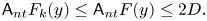 \[ {\mathsf{A}}_{nt} F_k(y) \leq {\mathsf{A}}_{nt} F (y) \le 2D. \]
Therefore, we deduce that for all sufficiently large  $N\gg 1$,
 \[ \frac{1}{4}\int F_k\,dm_Y \le \frac{1}{N} \bigg(\sum_{n=1}^{n_0} {\mathsf{A}}_{nt} F_k(y) +\sum_{n=n_0+1}^N {\mathsf{A}}_{nt} F_k (y) \bigg) \le \frac{k n_0}N +\frac{ 2D(N-n_0)}{N}. \]
By sending  $N\to \infty$, we get that for all $k>2$,
 \[ \int F_k\,dm_Y\le 8 D. \]
Since  $\{F_k:k=3,4,..\}$ is an increasing sequence of positive functions converging to $F$ point-wise, the monotone convergence theorem implies
 \[ \int F\, dm_Y=\lim_{k\to\infty} \int F_k\,dm_Y\le 8 D \]
as we claimed.
We remark that in [Reference Eskin, Margulis and MozesEMM98], the Markov operator  $\mathsf {A}_t$ was defined using the integral over the translates $\operatorname {SO}(2) a_t$, whereas we use the integral over the translates $U_{[-\rho,\rho ]}a_t$ of a horocyclic piece. The proof of the following proposition, which is an analogue of [Reference Eskin, Margulis and MozesEMM98, § 5.3], is the main reason for our digression from their definition, as the handling of the PS-measure on $U$ is more manageable than that of the PS-measure on $\operatorname {SO}(2)$ in performing change of variables.
Proposition 7.5 Let  $F:Y_0\to [2,\infty )$ be a locally bounded Borel function satisfying the following properties.
(a) There exists
$\sigma \ge 2$ such that for all $h\in B_H(2)$ and $y\in Y_0$,
\[ \sigma^{-1}F(y)\leq F(yh)\leq \sigma F(y). \]
(b) There exist
$t\geq 2$ and $D_0>0$ such that for all $y\in Y_0$ and $1\le \rho \le 2$,
where\[ {\mathsf{A}}_{t,\rho}F(y)\leq\frac{1}{8 \sigma \mathsf{p}_Y^{\delta_Y}} \cdot F(y)+D_0, \]
$\mathsf {p}_Y$ is as in (4.6).


Then
 \[ m_Y(F)\le 64 D_0\mathsf{p}_Y^{\delta_Y}. \]
In view of Lemma 7.3, Proposition 7.5 is an immediate consequence of the following.
Proposition 7.6 Let  $F$ be as in Proposition 7.5. Then for all $y\in Y_0$ and $n\geq 1$, we have
 \begin{equation} {\mathsf{A}}_{nt}F(y)\leq \frac{1}{2^{n}} F(y)+8D_0\mathsf{p}_Y^{\delta_Y}. \end{equation}
Proof. The main step of the proof is the following estimate.
Claim For any  $1\leq \rho \leq \frac 32$, $y\in Y_0$ and $n\in \mathbb {N}$, we have
 \begin{equation} {\mathsf{A}}_{(n+1)t,\rho}F(y)\leq \tfrac 12 {\mathsf{A}}_{nt, \rho+e^{-nt}}F(y)+\hat{D} \end{equation}
where  $\hat D:=4 D_0 \mathsf {p}_Y^{\delta _Y}$; recall that $e^{-nt}\leq 1/2$.
Let us first assume this claim and prove the proposition. We observe:
•
$\sum _{j\ge 1} e^{-jt}\leq 1/2$ (as $t\ge 2$);•
$({8 \sigma \mathsf {p}_Y^{\delta _Y}} )^{-1} \le 1/2$; and•
$D_0\le \hat D$.


Using the assumption (b) of Proposition 7.5 with  $\rho _n=1+\sum _{j=1}^{n-1} e^{-jt}$ ( $n\geq 2$), we deduce that for any $n\geq 2$,
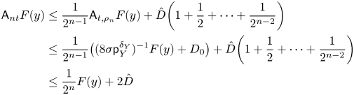 \begin{align} {\mathsf{A}}_{nt} F(y)& \leq \frac{1}{2^{n-1}} {\mathsf{A}}_{t, \rho_n}F(y)+\hat D\bigg(1+ \frac 12 +\cdots+ \frac 1{2^{n-2}}\bigg) \nonumber\\ &\leq \frac 1{2^{n-1}} \big((8 \sigma \mathsf{p}_Y^{\delta_Y})^{-1} F(y)+D_0\big)+\hat D\bigg(1+\frac 1{2} +\cdots+\frac 1{2^{n-2}}\bigg)\nonumber\\ &\leq \frac 1{2^{n}} F(y)+2\hat{D} \end{align}
which establishes the proposition.
We now prove the claim (7.8). For  $y\in Y_0$ and $\rho >0$, set
 \[ b_y(\rho):=\mu_{y}([-\rho,\rho])\quad\text{and}\quad b_y=b_y(1). \]
To ease the notation, we prove (7.8) with  $\rho =1$; the proof in general is similar. By assumption (a) and (b) of Proposition 7.5, we have
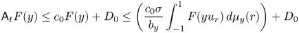 \begin{equation} {\mathsf{A}}_t F(y)\leq c_0F(y)+D_0 \leq \bigg(\frac{c_0\sigma }{b_y}\int_{-1}^1 F(yu_{r}) \,d\mu_{y}(r) \bigg)+D_0 \end{equation}
where  $c_0=({8 \sigma \mathsf {p}_Y^{\delta _Y}})^{-1}$.
Set  $\rho _n:=e^{-nt}$. Let $\{[r_j-\rho _n, r_j+\rho _n]: j\in J\}$ be a covering of
 \[ [-1,1]\cap {\rm supp}(\mu_{y}) \]
with  $r_j\in [-1,1]\cap {\rm supp}(\mu _{y})$ and with multiplicity bounded by $2$. For each $j\in J$, let $z_j:=yu_{r_j}$. Then
 \begin{equation} \sum_jb_{z_j}(\rho_n)=\sum_j\mu_y([r_j-\rho_n, r_j+\rho_n])\leq 2b_y(2). \end{equation}
Moreover, we get
 \begin{align} {\mathsf{A}}_{(n+1)t} F(y)&=\frac{1}{b_y}\int_{-1}^1 F(yu_{r}a_{(n+1)t})\,d\mu_{y}{}(r)\nonumber\\ &\leq\frac{1}{b_y}\sum_j\int_{-\rho_n}^{\rho_n}F(z_ju_{r}a_{(n+1)t})\,d\mu_{{z_j}}{}(r)\nonumber\\ &=\frac{1}{b_y}\sum_j\int_{-\rho_n}^{\rho_n}F(z_ja_{nt}u_{re^{nt}}a_t)\,d\mu_{z_j}{}(r). \end{align}
We now make the change of variables  $s=re^{nt}$. In view of (7.12), we have
 \[ {\mathsf{A}}_{(n+1)t} F(y)\leq\frac{1}{b_y}\sum_j\frac{b_{z_j}(\rho_n)}{b_{z_ja_{nt}}}\int_{-1}^1F(z_ja_{nt}u_{s}a_t)\,d\mu_{z_ja_{nt}}{}(s). \]
Applying (7.10) with the base point  $z_ja_{nt}$, we get from the above that
 \begin{align} {\mathsf{A}}_{(n+1)t} F(y)&\leq\frac{1}{b_y}\sum_j\frac{b_{z_j}(\rho_n)c_0\sigma}{b_{z_ja_{nt}}}\int_{-1}^1 F(z_ja_{nt}u_{s})\,d\mu_{z_ja_{nt}}{}(s)\nonumber\\ &\quad +\frac{1}{b_y}\sum_jb_{z_j}(\rho_n)D_0. \end{align}
By (7.11), we have  $({1}/{b_y})\sum _jb_{z_j}(\rho _n)D_0\leq \hat D.$
Therefore, reversing the change of variable, i.e. now letting  $r=e^{-nt}s$, we get from (7.13) the following:
 \begin{align*} {\mathsf{A}}_{(n+1)t} F(y)&\leq \frac{1}{b_y}\sum_j c_0\sigma\int_{-\rho_n}^{\rho_n} F(z_ju_{r}a_{nt}) \,d\mu_{z_j}{}(r)+\hat{D}\\ &\leq \frac{2c_0\sigma}{b_y}\int_{-(1+\rho_n)}^{1+\rho_n} F(yu_{r}a_{nt}) \,d\mu_{y}{}(r)+\hat{D}\\ &=\frac{2c_0\sigma b_y(1+\rho_n)}{b_y } {\mathsf{A}}_{nt, 1+\rho_n}F(y) +\hat{D}. \end{align*}
Since
 \[ \sup_{y\in Y_0} \frac{2c_0\sigma b_y(2)}{b_y}= ({4 \mathsf{p}_Y^{\delta_Y}})^{-1} \sup_{y\in Y_0} \frac{ b_y(2)}{b_y} \le \frac 12, \]
we get
 \[ {\mathsf{A}}_{(n+1)t} F(y) \le \tfrac{1}{2} {\mathsf{A}}_{nt, 1+\rho_n}F(y) +\hat D . \]
The proof is complete.
8. Return lemma and number of nearby sheets
We fix closed non-elementary  $H$-orbits $Y$ and $Z$ in $X$. Since $Z$ is closed, a fixed ball around $y\in Y_0$ intersects only finitely many sheets of $Z$ (see Figure 2). The aim of this section is to show that the number of sheets of $Z$ in $B(y, \operatorname {inj} (y))$ is controlled by the tight area of $S_Z$ with a multiplicative constant depending on $\mathsf {p}_Y$ and $\delta _Y$.
The main ingredient is a return lemma which says that for any  $y\in Y_0$, there exists some point in $\{yu_r\in Y_0: r\in [-1,1]\}$ whose minimum return time to a fixed compact subset under the geodesic flow is comparable to $\log (\omega (y))$ (see Lemma 8.4).
Return lemma
We use the notation of § 6.
Recall that  ${\rm Lie}(G)=i\mathfrak {sl}_2(\mathbb {R})\oplus \mathfrak {sl}_2(\mathbb {R})$. We define a norm $\|\cdot \|$ on $\operatorname {Lie}(G)$ using an inner product with respect to which $\mathfrak {sl}_2(\mathbb {R})$ and $i\mathfrak {sl}_2(\mathbb {R})$ are orthogonal to each other. Given a vector $w\in {\rm Lie}(G)$, we write
 \[ w=i {\rm Im}(w)+{\rm Re}(w)\in i\mathfrak{sl}_2(\mathbb{R})\oplus \mathfrak{sl}_2(\mathbb{R}). \]
Since the exponential map  ${\rm Lie} (G) \to G$ defines a local diffeomorphism, there exists an absolute constant $c_1\ge 2$ satisfying the following two properties.
(1) For all
$x\in X$, and all $w=i{\rm Im}(w)+{\rm Re}(w)\in \operatorname {Lie}(G)$ with $\|w\| \le \max (1, {\varepsilon }_X)$,
(8.1)\begin{equation} c_1^{-1}\|w\|\leq d(x,x\exp(i {\rm Im}(w))\exp({\rm Re}(w)))\leq c_1\|w\|. \end{equation}(2) If
$d(x,x')\leq {\varepsilon }_X/c_1$, then $x'=x\exp (i {\rm Im}(w))\exp ({\rm Re}(w))$ for some $w\in {\rm Lie}(G)$.


We choose an absolute constant  $d_X\ge 24$ so that
 \[ X_{{\varepsilon}_X}\subset \{x\in X_0: \omega(x)\le d_X\}. \]
Let  $D_1:=D_1(Y)$ be given by
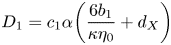 \begin{equation} D_{1}= c_1 \alpha \bigg(\frac{6{b_1}}{\kappa \eta_0} +d_X \bigg) \end{equation}
where  $\kappa$ is defined by $\hat {b}_0 \mathsf {p}_Y^{\delta _Y} \kappa ^{\delta _Y/2}=1/2$, $0<\eta _0 <1$ is as in (6.6), $\alpha \ge 1$ is as in (6.8), and $c_1$ is as in (8.1). We note that by increasing $\hat {b}_0$ if necessary, we may and will assume that $\kappa \in (0,1)$. Moreover, we put $\eta _0=\frac 12$ when $Y$ is convex cocompact.
Define
 \begin{equation} \mathcal{K}_Y=\{y\in Y_0: \omega(y)\leq D_{1} /(c_1\alpha)\}. \end{equation}
Note that  $X_{{\varepsilon }_X}\cap Y_0 \subset \mathcal {K}_Y$.
The choices of the above parameters are motivated by our applications in the following lemmas. Indeed the choice of  $\kappa$ is used in (8.6). The multiplicative parameter $c_1\alpha$, which features in the definitions of ${D_1}$ and $\mathcal {K}_Y$, is tailored so that we may utilize Lemma 8.10 in the proof of Lemma 8.13.
Lemma 8.4 (Return lemma)
For every  $y\in Y_0$, there exists some $|r|\leq 1$ so that $yu_ra_{-t}\in \mathcal {K}_Y$ where $t=\log (\eta _0\omega (y)/6)$.
Proof. Let  $y\in Y_0-\mathcal {K}_Y$. By the definition of $\omega$, there exist $1\le i\le \ell$ and $g\in \tilde {\mathfrak {h}}_i$ so that $y=[g]$ and
 \[ \omega(y)=\omega_i(y), \]
see § 6 for the notation. Set  $v:= v_i g$. Then
 \[ \|v\|^{-1}=\omega_i(y)=\omega(y). \]
Let us write  $v=w+se_3$ where $w\in V$ and $s\in \mathbb {R}$. Recall from Lemma 5.12 that there exists $b_1>1$ so that
 \begin{equation} \|w\|\geq b_1^{-1}\|v\|. \end{equation}
 Let  $\kappa >0$ be as used in (8.2). Then (5.5) implies that
 \begin{equation} \mu_{y}\bigg(D^+\bigg(\frac{w}{\|w\|},\kappa\bigg)\bigg)\leq \frac{1}{2}\mu_y([-1,1]). \end{equation}
Therefore, there exists  $r\in {\rm supp}(\mu _y)\cap \big ([-1,1]- D^+( {w}/{\|w\|},\kappa )\big )$. This means that $yu_r\in Y_0$, moreover, we have, using (8.5),
 \[ \|p^+(vu_{r})\|=\|p^+(wu_{r})\|>\kappa\|w\| \geq \kappa b_1^{-1}\|v\|. \]
Set  $t:=\log (\eta _0 \omega (y)/ 6)$. Then
 \begin{align*} \kappa b_1^{-1}{\|v\|} \cdot\frac{ \eta_0 \omega(y)}{6} &= \kappa b_1^{-1}{\|v\|} e^t \le \|p^+(vu_r)a_t\| \\ &\le \| v u_{r} a_t\|\le \|vu_r\|e^t\le 2\|v\| \cdot\frac{ \eta_0 \omega(y)}{6}, \end{align*}
where we use  $\|vu_r\|\leq 2\|v\|$ in the last inequality.
Hence, using the fact that  $\omega (y)=\|v\|^{-1}$,
 \[ \frac{\kappa b_1^{-1}\eta_0}{6 }\le \| v u_{r} a_t\|=\|v_i g u_ra_t\|\le \frac{\eta_0}3. \]
This in particular implies that  $gu_ra_t\in \tilde {\mathfrak {h}}_i$. By Lemma 6.5, whenever $\gamma \in \Gamma$ and $1\leq j\leq \ell$ satisfy that $\tilde {\mathfrak {h}}_j\neq \gamma \tilde {\mathfrak {h}}_i$, we have
 \[ \| v_j \gamma g u_ra_t\| \ge \eta_0; \]
note that  $i=j$ is allowed.
This and the above upper bound thus imply
 \[ \omega(yu_ra_t) = \|v_i g u_ra_t\|^{-1}. \]
Therefore,
 \[ \omega (yu_ra_t) \le \frac{6b_1}{\kappa \eta_0}\le D_1/(c_1\alpha) \]
proving the claim.
Number of nearby sheets
Recalling that  $\mathfrak {sl}_2(\mathbb {C})=\mathfrak {sl}_2(\mathbb {R}) \oplus i\mathfrak {sl}_2(\mathbb {R})$, we set $V=i\mathfrak {sl}_2(\mathbb {R})$ and consider the action of $H$ on $V$ via the adjoint representation; so $v\cdot h= h^{-1} v h$ for $v\in V$ and $h\in H$. We use the relation $g (\exp v) h= gh \exp (v\cdot h)$ which is valid for all $g\in G, v\in V, h\in H$.
If  $D\ge \alpha /2$ for $\alpha$ as in Proposition 6.7, then $D^{-1}\omega (y)^{-1}\le \tfrac 12 \operatorname {inj} (y)$.
Definition 8.7 For  $y\in Y_0$ and $D\ge \alpha /2$, we define
 \begin{equation} I_Z(y,D)=\{v\in V-\{0\}: \|v\|< D^{-1}\omega(y)^{-1},\; y\exp(v)\in Z\}. \end{equation}
 Since  $V$ is the orthogonal complement to ${\rm Lie} (H)$, the set $I_Z(y, D)$ can be understood as the number of sheets of $Z$ in the ball around $y$ of radius $D^{-1}\omega (y)^{-1}$.
It turns out that  $\# I_Z(y, D)$ can be controlled in terms of the tight area of $S_Z$, uniformly over all $y\in Y_0$ for an appropriate $D>1$.
Notation 8.9 We set
 \begin{align*} \tau_Z :=\operatorname{area}_t(S_Z). \end{align*}
Theorem 3.3 shows that  $1\ll \tau _Z<\infty$ where the implied constant depends only on $M$.
$M$.
We begin with the following lemma.
Lemma 8.10 With  $c_1\ge 2$ and $\alpha \ge 2$ given respectively in (8.1) and (6.7), we have that for all $y\in Y_0$,
 \begin{equation} \# I_Z(y, c_1 \alpha) \ll \omega(y)^{3} \tau_Z .\end{equation}
Proof. Let  $c_1\ge 1$ and $\alpha$ be the absolute constants given in (8.1) and (6.7) respectively. It follows that for any $y\in Y_0$ and $v\in I_Z(y,\alpha )$,
 \begin{equation} d(y,y\exp(v))\leq c_1\|v\| \leq c_1(c_1\alpha)^{-1} \cdot \omega(y)^{-1} <\tfrac{1}{2} \cdot {\operatorname{inj}(y)}. \end{equation}
 It follows that for each  $v\in I_Z(y, c_1\alpha )$, $\operatorname {inj}(y\exp v)\ge {\operatorname {inj} (y)}/{2}$. Hence the balls $B_Z(y\exp v, {\operatorname {inj}(y)}/{2})$, $v\in I_Z(y,c_1 \alpha )$ are disjoint from each other, and hence
 \[ \# I_Z(y, \alpha) \cdot \operatorname{Vol}(B_H(e, {\operatorname{inj}(y)}/{2})) =\operatorname{Vol}\biggl\{\bigcup B_Z(y\exp v, {\operatorname{inj}(y)}/{2}) :v\in I_Z(y, \alpha)\biggr\}. \]
On the other hand, if we set  $\rho _y:=\min \{1, \operatorname {inj}(y)/2\}$, then
 \[ \pi\biggl(\biggl\{\bigcup B_Z(y\exp v, \rho_y) :v\in I_Z(y, c_1\alpha)\biggr\}\biggr)\subset S_Z\cap\mathcal{N}({\operatorname{core}}\,(M)). \]
Therefore
 \[ \# I_Z(y, c_1\alpha) \le \operatorname{Vol}(B_H(e, \rho_y))^{-1} \cdot \tau_Z\ll \rho_y^{-3}\tau_Z\ll \omega(y)^{3} \tau_Z ; \]
we have used that  $2\pi (\cosh r -1)\ge r^3$ for all $r>0$ and Proposition 6.7 respectively in the last two estimates.
Let  $D_1$ be as in (8.2). By the choice of $\kappa$, we have $D_1\ll \mathsf {p}_Y^2$ (see the discussion following (8.2)).
Lemma 8.13 (Number of sheets)
For  $D_1=D_1(Y)\ll \mathsf {p}_Y^2$ as in (8.2), we have
 \[ \sup_{y\in Y_0} \#I_Z(y,{D_1})\le c_0\cdot {\mathsf{p}}_Y^{6} \cdot \tau_Z \]
where  $c_0\geq 2$ is an absolute constant.
Proof. Let  $\mathcal {K}_Y$ be as in (8.3):
 \[ \mathcal{K}_Y=\{y\in Y_0: \omega(y)\leq (c_1\alpha)^{-1} {D_1}\}. \]
If  $y\in \mathcal {K}_Y$, then, by Lemma 8.10,
 \[ \#I_Z(y, {D_1}) \le \#I_Z(y,c_1\alpha)\ll D_1^3 \tau_Z\ll \mathsf{p}_Y^6\tau_Z . \]
Now suppose that  $y\in Y_0-\mathcal {K}_Y$. By Lemma 8.4, there exist $|r|<1$ and $t=\log (\eta _0\cdot \omega (y)/6)$, where $0<\eta _0\leq 1$ is as in (6.6), such that
 \[ yu_ra_t \in \mathcal{K}_Y. \]
We claim that if  $v\in I_Z(y,{D_1})$, then $v(u_{r}a_{t}) \in I_Z(yu_ra_t, c_1\alpha )$. Firstly, note that, plugging $t=\log (\eta _0\cdot \omega (y)/6)$ and using $0<\eta \le 1$,
 \[ \|v(u_ra_{t})\| \leq 3 e^t \|v\| = \frac{3\eta_0\, \omega(y)\, \|v\|}{6} < \omega(y) \cdot \|v\|. \]
Hence for  $v\in I_Z(y,{D_1})$, as $\omega (y) \|v\|< D_1^{-1}$,
 \[ \|v (u_ra_{t})\|< \omega(y) \cdot \|v\|\le D_1^{-1}\leq (c_1\alpha)^{-1}\omega(yu_ra_t)^{-1}. \]
where we used the fact that  $(c_1\alpha )^{-1}{D_1} > \omega (yu_ra_t)$.
Since  $y(\exp v) u_{r}a_{t} = (y u_ra_t)\exp (v(u_{r}a_t)) \in Z$, this implies that $v(u_{r}a_{t}) \in I_Z(yu_ra_t, c_1\alpha )$. Therefore the map $v\mapsto v(u_{r}a_{t})$ is an injective map from $I_Z(y,{D_1})$ into $I_Z(yu_ra_t, c_1\alpha )$. Consequently,
 \[ \#I_Z(y, {D_1})\le \#I_Z(yu_ra_t, c_1\alpha) \ll {\mathsf{p}}_Y^{6} \cdot \tau_Z. \]
This finishes the proof.
9. Margulis function: construction and estimate
Throughout this section, we fix closed non-elementary  $H$-orbits $Y, Z$ in $X$ and
 \[ \frac{\delta_Y}{3}\le s< {\delta_Y}. \]
In this section, we define a family of Margulis functions  $F_{s, \lambda }=F_{s,\lambda, Y, Z}$, $\lambda >1$ and show that the hypothesis of Proposition 7.5 is satisfied for a certain choice of $\lambda$, which we will denote by $\lambda _s$. As a consequence, we will get an estimate on $m_Y(F_{s, \lambda _s})$ in Theorem 9.18.
We set
 \[ I_Z(y):=\{v\in V-\{0\}: \|v\|< D_1^{-1}\omega(y)^{-1},\; y\exp(v)\in Z\} \]
for  $D_1>1$ as given in Lemma 8.13.
Definition 9.1 (Margulis function)
(1) Define
$f_s:=f_{s,Y, Z}:Y_0 \to (0,\infty )$ by
\[ f_s(y):=\begin{cases}\sum_{v\in I_Z(y)}\|v\|^{-s} & \text{if $I_Z(y)\ne \emptyset$,}\\ \omega(y)^{s} & \text{otherwise}.\end{cases} \]
(2) For
$\lambda \ge 1$, define $F_{s,\lambda }=F_{s, \lambda, Y, Z}:Y_0\to (0,\infty )$ as follows:
(9.2)\begin{equation} F_{s, \lambda}(y)=f_{s}(y)+\lambda \;\omega (y)^s. \end{equation}


Note that for all  $y\in Y_0$
 \begin{equation} \omega(y)^{s} \le f_s(y)<\infty. \end{equation}
Since  $Y$ and $Z$ are closed orbits, both $f_s$ and $F_{s,\lambda }$ are locally bounded. Moreover, they are also Borel functions. Indeed, $\omega ^s$ is continuous on $Y_0$, and $f_s$ is continuous on the open subset $\{y\in Y_0: I_Z(y)\neq \emptyset \}$ as well as on its complement.
In this section, we specify choices of parameters  $t_s$ and $\lambda _s$ so that the average ${\mathsf {A}}_{t_s}F_{s, \lambda _s}$ satisfies the hypothesis of Proposition 7.5 with controlled size of the additive term (Lemma 9.14).
Notation 9.4 (Parameters)
(1) For
$0< c <1$, define $t(c, s)>0$ by
where\[ \frac{ b_0 b_1 {\mathsf{p}}_Y^{\delta_Y} e^{-(\delta_Y -s)t(c,s) /4} }{(\delta_Y-s)}= c \]
$b_0$ and $b_1$ are given in Lemma 5.13.(2) For
$0< c<1$ and $t>0$, define $\lambda (t,c,s)>0$ by
where\[ \lambda(t,c,s):=\big( 2 c_0 D_1 p_Y^{6}\tau_Z\big) \frac{ e^{2ts}}{c} \]
$c_0$ is given by (8.13).


As it is evident from the above, the definition of  $t(c,s)$ is motivated by the linear algebra Lemma 5.13. Indeed, for any vector $v\in e_1G$ and $t\ge t(c,s)$, we have
 \begin{equation} \sup_{1\le \rho\le 2} \frac{1}{\mu_y[-\rho,\rho]}\int_{-\rho}^{\rho} \frac{1}{\| vu_r a_t\|^{s}} \,d\mu_{y}{} (r)\le {c\|v\|^{-s}}. \end{equation}
 The choice of  $\lambda (t,c,s)$ is to control the additive difference between $f_s(yu_ra_t )$ and $\sum _{v\in I_Z(y) }\|vu_ra_t\|^{-s}$ uniformly over all $r\in [-1,1]$ such that $yu_r\in Y_0$, so that we will get
 \[ {\mathsf{A}}_{t} f_{s}(y) \le c\cdot f_{s}(y)+ \frac{\lambda (t,c,s) c}{2} \omega(y)^{s} \]
(see Lemma 9.11, (9.15) and (9.16)).
Markov operator for the height function
In this subsection, we use notation from § 6.
It will be convenient to introduce the following notation.
Notation 9.6 Let  $Q\subset G$ be a compact subset.
(1) Let
$d_Q\geq 1$ be the infimum of all $d\geq 1$ such that for all $g\in Q$ and $v\in \mathbb {R}^4$,
(9.7)Note that\begin{equation} d^{-1} \|v\| \le \| vg \|\le d \|v\|. \end{equation}$d_Q\asymp \max _{g\in Q} \|g\|$, up to an absolute multiplicative constant.(2) We also define
$c_Q\geq 1$ to be the infimum of all $c\geq 1$ such that for any $x\in X_0$, $g\in Q$ with $xg\in X_0$, and for all $1\le i \le \ell$
(9.8)We note that\begin{equation} c^{-1} \omega_i(x) \le \omega_i(xg)\le c\, \omega_i(x). \end{equation}$c_Q\asymp \max _{g\in Q} \|g\|$ up to an absolute multiplicative constant.


Lemma 9.9 For any  $0< c\leq 1/2$ and $t \ge t(c, s)$, there exists $D_2\asymp e^{2t}$ so that for all $y\in Y_0$ and $1\leq \rho \leq 2$,
 \[ {\mathsf{A}}_{t,\rho} \omega (y)^s\le c \cdot \omega(y)^s+D_2. \]
Proof. Let  $t\geq t(c, s)$. We compare $\omega (yu_ra_t)$ and $\omega (y)$ for $r\in [-2,2]$. Setting
 \[ Q:= \{a_\tau u_r :|r|\leq 2, |\tau|\leq t\}, \]
we have  $c_Q \asymp e^t$.
Let  $\eta _0$ be as in Lemma 6.5. Fix $0<\eta _X\leq \min \{{\varepsilon }_X,\eta _0\}$ so that
 \[ \eta_X\asymp {\varepsilon}_X\quad\text{and}\quad\eta_X^{-1}\geq \sup_{y\in X_{{\varepsilon}_X}\cap Y_0} \omega(y). \]
We consider two cases.
Case 1:  $\omega (y)\leq 2c_Q/\eta _X$. In this case, for $h\in Q$ with $yh\in Y_0$,
 \[ \omega(yh)\leq 2c_Q^2/\eta_X. \]
Hence, the claim in this case follows if we choose  $D_2=2c_Q^2/\eta _X\asymp e^{2t}$.
Case 2:  $\omega (y) >2c_Q/\eta _X$. By the definition of $\omega$, there exists $1\le i\le \ell$ such that
 \[ \omega_i(y)>2c_Q/\eta_X,\quad\text{ and hence}\quad y\in \mathfrak{h}_{i}. \]
By the definition of  $c_Q$, see (9.8), we have
 \[ \omega_i(yh)>2/\eta_X,\quad\text{and hence}\quad yh\in \mathfrak{h}_{i} \]
for all  $h\in Q$ with $yh\in Y_0$. Choose $g_0\in G$ so that $y=[g_0]$. In view of Lemma 6.5, see in particular (6.6), and since $\eta _X\leq \eta _0$ there exists $\gamma \in \Gamma$ such that simultaneously for all $h\in Q$ with $yh\in Y_0$,
 \[ \omega(yh)=\omega_i(yh)=\|v_{i}\gamma g_0h\|^{-1}. \]
Since  $v_i=e_1g_i^{-1} \in e_1G$ (see (6.1)), we may apply Lemma 5.13 (linear algebra lemma II) and deduce
 \begin{align*} {\mathsf{A}}_{t,\rho}\omega(y)^s&=\frac{1}{\mu_y([-\rho,\rho])}\int_{-\rho}^{\rho} \frac{1}{\| v_{i}\gamma u_r a_t \|^s} \,d\mu_y(r)\\ &\leq \frac{ b_0b_1{\mathsf{p}}_Y^{\delta_Y} e^{-(\delta_Y-s) t/4 } }{(\delta_Y-s)} \|v_{i}\gamma\|^{-s}\le c\cdot \omega(y)^s; \end{align*}
in the last inequality we used the fact that  $t\geq t(c,s)$. The proof is now complete.
Log-continuity of $F_{s,\lambda }$

The following log-continuity lemma with a control on the multiplicative constant  $\sigma$ is the first hypothesis in Proposition 7.5.
Lemma 9.10 (Log-continuity lemma)
There exists  $2\le \sigma \ll {\mathsf {p}}_Y^{8}$ so that the following holds: for every $\lambda \geq \tau _Z$, we have
 \[ \sigma^{-1} F_{s,\lambda} (y) \le F_{s,\lambda}(yh) \le \sigma F_{s,\lambda}(y) \]
for all  $y\in Y_0$ and all $h\in B_H(2)$ so that $yh\in Y_0$.
Let  $c_0$ be as in Lemma 8.13. Recall from Theorem 3.3 that $\tau _Z\geq {\varepsilon }_X^2$, replacing $c_0$ by its multiple (which we continue to denote by $c_0$) if necessary we assume that $c_0\tau _Z\geq 1$.
We first obtain the following estimate for  $f$ on nearby points.
Lemma 9.11 Let  $Q\subset H$ be a compact subset. For any $y\in Y_0$ and $h\in Q$ such that $yh\in Y_0$, we have
 \[ f_{s}(yh)\le \sum_{v\in I_Z(y)} \|vh \|^{-s} +{}\big( {c_0} c_Q d_Q D_1 {\mathsf{p}}_Y^{6} \tau_Z \big) \omega(y)^s \]
where  $c_0$ is as above and the sum is understood as $0$ when $I_Z(y)=\emptyset$.
Proof. Let  $y\in Y_0$ and $h\in Q$ with $yh\in Y_0$. If $I_Z(yh)=\emptyset$, then by (9.8), we have
 \[ f_{s}(yh)= \omega(yh)^{s} \le c_Q ^s \omega(y)^{s} \]
proving the claim; recall that  $c_0\tau _Z\geq 1$.
Now suppose that  $I_Z(yh)\ne \emptyset$. Setting
 \[ {\varepsilon}:=( d_Q D_1 \omega(y))^{-1}, \]
we write
 \begin{equation} f_{s}(yh) = \sum_{v\in I_Z(yh), \|v\|< \varepsilon}\|v\|^{-s}+\sum_{v\in I_Z(yh), \|v\|\geq \varepsilon}\|v\|^{-s} . \end{equation}
 Since  $\# I_Z(yh)\le c_0 {\mathsf {p}}_Y^{6} \tau _Z$ by Lemma 8.13, we have
 \begin{equation} \sum_{v\in I_Z(yh), \|v\|\geq \varepsilon}\|v\|^{-s}\leq \bigl(c_0 {\mathsf{p}}_Y^{6}\tau_Z\bigr)\varepsilon^{-s}\le \bigl(c_0 d_Q D_1 {\mathsf{p}}_Y^{6}\tau_Z \bigr)\omega(y)^{s}. \end{equation}
 Thus, if there is no  $v\in I_Z(yh)$ with $\|v\|\le {\varepsilon }$, then the lemma follows from (9.12).
If  $v\in I_Z(yh)$ satisfies $\|v\|< \varepsilon$, then
 \[ \|vh^{-1} \|\leq d_Q \varepsilon=D_1^{-1} \omega(y)^{-1}; \]
in particular,  $vh^{-1}\in I_Z(y)$. Therefore, by setting $v'=vh^{-1}$,
 \[ \sum_{v\in I_Z(yh), \|v\|< \varepsilon}\|v\|^{-s}\le \sum_{v'\in I_Z(y)}\|v' h\|^{-s}. \]
Together with (9.13), this finishes the proof.
Proof of Lemma 9.10 Since  $B_H(2)^{-1}=B_H(2)$, it suffices to show the inequality $\le$. By Lemma 9.11, applied with $Q=B_H(2)$, $c:=c_{B_H(2)}$ and $d:=d_{B_H(2)}$, we have that for all $h\in B_H(1)$ with $yh\in Y_0$, we have
 \begin{align*} f_{s}(yh)&\le \sum_{v\in I_Z(y)} \|vh \|^{-s} +{}\big( {c_0} c d D_1 {\mathsf{p}}_Y^{6} \tau_Z \big) \omega(y)^s \\ &\leq d \sum_{v\in I_Z(y)} \|v\|^{-s} +{}c_0c d D_1 {\mathsf{p}}_Y^{6}\tau_Z \omega(y)^s, \end{align*}
where we have used the definition of  $d$.
$d$.
Recall from Theorem 3.3 that  ${\varepsilon }_X^2\leq \tau _Z\leq \lambda$ and that $D_1\ll \mathsf {p}_Y^2$.
If  $I_Z(y)=\emptyset$, then
 \begin{align*} F_{s,\lambda}(yh)&\ll {\mathsf{p}}_Y^8 \tau_Z\omega (y)^s+\lambda \omega(y)^s\ll \mathsf{p}_Y^{8} \lambda \omega(y)^s\\ &\ll {\mathsf{p}}_Y^{8} (f_{s}(y) + \lambda \omega(y)^s)\ll{\mathsf{p}}_Y^{8} F_{s,\lambda}(y). \end{align*}
If  $I_Z(y)\ne \emptyset$, then
 \begin{align*} F_{s,\lambda}(yh)&\leq d\cdot f_{s}(y)+ {}c_0c d D_1 {\mathsf{p}}_Y^{6}\tau_Z \omega(y)^s +\lambda\omega(yh)^s\\ &\ll f_{s}(y)+\mathsf{p}_Y^{8} \lambda\omega(y)^s \ll \mathsf{p}_Y^{8} F_{s,\lambda}(y). \end{align*}
This finishes the upper bound. The lower bound can be obtained similarly.
Main inequality
We will apply the following lemma to obtain the second hypothesis of Proposition 7.5 for  $c:=(8\sigma \mathsf {p}_Y^{\delta _Y})^{-1}<1/2$.
Lemma 9.14 (Main inequality)
Let  $0< c\leq 1/2$. For $t\geq t(c/2,s)$ and $\lambda =\lambda (t,c,s)$, we have the following: for any $y\in Y_0$ and $1\leq \rho \leq 2$, we have
 \[ {\mathsf{A}}_{t,\rho} F_{s,\lambda} (y)\le c \, F_{s,\lambda}(y)+\lambda {D_2} \]
where  ${D_2} \ll e^{2t}$ is as in Lemma 9.9.
Proof. The following argument is based on comparing the values of  $f_{s}(yu_ra_t)$ and $f_{s}(y)$ for $r\in [-2,2]$ such that $yu_ra_t\in Y_0$.
Let  $Q:=\{a_\tau u_r: |r| \le 2 , |\tau |\leq t\}$. Then
 \[ c_Q {\asymp}e^t\quad\text{and}\quad d_Q {\asymp}e^{t} \]
where  $c_Q$ and $d_Q$ are as in (9.6). Hence, by Lemma 9.11, we have that for any $|r|\le 2$ such that $yu_ra_t\in Y_0$,
 \begin{equation} f_{s}(yu_ra_t)\le \sum_{v\in I_Z(y)} \|v u_ra_t\|^{-s} + c_0 D_1 {\mathsf{p}}_Y^{6} \tau_Z \omega(y)^s e^{2ts} \end{equation}
where  $c_0$ is as in Lemma 9.11.
By averaging (9.15) over  $[-\rho,\rho ]$ with respect to $\mu _y$, and applying (9.5), we get
 \begin{align} {\mathsf{A}}_{t,\rho} f_{s}(y)&\leq c\cdot f_{s}(y)+ c_0 D_1 {\mathsf{p}}_Y^{6} \tau_Z \omega(y)^{s} e^{2ts} \nonumber\\ &\leq c\cdot f_{s}(y)+ \frac{\lambda c}{2} \omega(y)^{s}. \end{align}
Then by Lemma 9.9 and (9.16), we have
 \begin{align*} {\mathsf{A}}_{t,\rho} F_{s,\lambda}(y) & = {\mathsf{A}}_{t,\rho} f_{s}(y)+ {\mathsf{A}}_{t,\rho} \lambda\omega(y)^s \\ &\leq c\cdot f_{s}(y)+\frac{c\lambda}{2}\omega(y)^{s}+\frac{c\lambda}{2}\omega(y)^{s}+\lambda D_2\\ &=c\cdot F_{s,\lambda}(y)+\lambda D_2. \end{align*}
By Theorem 4.8, we have  $\mathsf {s}_Y\asymp {\mathsf {p}}_Y$. For the sake of simplicity of notation, we put
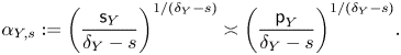 \begin{equation} \alpha_{Y,s}:=\bigg(\frac{{\mathsf{s}}_Y}{ \delta_Y-s}\bigg) ^{1/ (\delta_Y-s)} \asymp \bigg(\frac{{\mathsf{p}}_Y}{ \delta_Y-s}\bigg) ^{1/ (\delta_Y-s)}.\end{equation}
We are now in a position to apply Proposition 7.5 to get the following estimate.
Theorem 9.18 (Margulis function on average)
There exists  $\lambda _s>1$ such that
 \[ m_Y(F_{s, \lambda_s}) \ll \alpha_{Y,s}^\star \tau_Z. \]
Proof. Let  $1\leq \sigma \ll \mathsf {p}_Y^8$ be given by Lemma 9.10. Let $c:=(8\sigma \mathsf {p}_Y^{\delta _Y})^{-1}<1/2$, $t_s:= t(c, s)$ and $\lambda _s:=\lambda ( t_s,c, s)$ be given by (9.4). Then in view of Lemmas 9.10 and 9.14, $F_{s,\lambda _s}$ satisfies the conditions of Proposition 7.5 with $t=t_s$ and $D_0=\lambda _s D_2$, where $D_2\ll e^{2t_s}$ is given in Lemma 9.9. Therefore
 \begin{equation} m_Y(F_{s, \lambda_s})\le 64\lambda_s \mathsf{p}_Y^{\delta_Y}D_2. \end{equation}
Since
 \[ e^{(\delta_Y -s)t_s } =\frac{ (8\sigma b_0 b_1 {\mathsf{p}}_Y^{2\delta_Y})^4 }{(\delta_Y-s)^4} \ll \bigg(\frac{ {\mathsf{p}}_Y }{\delta_Y-s} \bigg)^{\star} \quad\text{and} \quad \lambda_s=\big( 2 c_0 D_1 p_Y^{6}\tau_Z\big) \frac{ e^{2t_s s}}{c}, \]
we get
 \[ \lambda_s \mathsf{p}_Y^{\delta_Y}D_2 \ll \mathsf{p}_Y^\star e^{4t_s} \tau_Z\ll\alpha_{Y,s}^\star \tau_Z. \]
Combining this with (9.19) finishes the proof.
10. Quantitative isolation of a closed orbit
In this section, we deduce Theorem 1.5 from Theorem 9.18. Let  $Y, Z$ be non-elementary closed $H$-orbits in $X$. We allow the case $Y=Z$ as well. Let $ {\delta _Y}/{3} \le s< \delta _Y$.
Recall the definitions of  $f_s=f_{s,Y, Z}$ and $F_{s,\lambda }=F_{s,\lambda, Y, Z}$ from Definition 9.1. Let $\lambda _s$ be given by Theorem 9.18. Using the log-continuity lemma for $F_{s,\lambda _s}$ (Lemma 9.10), we first deduce the following estimate.
Proposition 10.1 For any  $0<\varepsilon <{\varepsilon }_X$ and $y\in Y_0\cap X_\varepsilon$, we have
 \[ f_{s, Y, Z}(y)\le F_{s,\lambda_s}(y)\ll \frac{\alpha_{Y, s}^\star \tau_Z }{m_Y(B(y, {\varepsilon}))}. \]
Proof. Let  $y\in Y_0\cap X_{\varepsilon }$. Then $\operatorname {inj}(y)\ge {\varepsilon }$ and hence $y B_H({\varepsilon })= B(y, {\varepsilon })$. For all $h\in B_H({\varepsilon }_X)$, $F_{s,\lambda _s} (y) \le \sigma F_{s,\lambda _s}(yh)$ for some constant $\sigma \ll \mathsf {p}_Y^{6}$ by Lemma 9.10. By applying Theorem 9.18, we get
 \[ F_{s, \lambda_s} (y) \le \frac{ \sigma \int_{x\in y B_H({\varepsilon})} F_{s,\lambda_s}(x) \,dm_Y(x)}{m_Y(B(y, {\varepsilon}))}\le \frac{ \sigma \cdot m_Y(F_{s,\lambda_s})}{m_Y(B(y, {\varepsilon}))} \ll \frac{\alpha_{Y, s}^\star \tau_Z }{m_Y(B(y, {\varepsilon}))}. \]
Recall from (6.8) that for all  $x\in X_0$,
 \begin{equation} \frac{1}{2\alpha} \cdot \operatorname{inj} (x)\le \omega(x)^{- 1} \le \frac{\alpha}{2} \cdot \operatorname{inj} (x). \end{equation}
 Using the next lemma, we will be able to use the estimate for  $f_{s, Y, Z}$ obtained in Proposition 10.1 to deduce a lower bound for $d(y, Z)$.
Lemma 10.3
(1) Let
$y\in Y_0$ and $z\in Z- B_Y(y, \operatorname {inj}(y))$. If $d(y, z) \le ({1}/{2\alpha c_1D_1})\operatorname {inj}(y)$, then
where\[ d(y, z)^{-s}\le c_1 f_{s, Y, Z}(y) \]
$c_1\ge 1$ is as in (8.1).(2) If
$Y\ne Z$, then for any $y\in Y_0$,
\[ d(y, Z)^{-s} \ll \mathsf{p}_Y^2 f_{s,Y, Z}(y). \]


Proof. As  $Z$ is closed and $d(y, z) \le ({1}/{2\alpha c_1D_1})\operatorname {inj} (y) <\frac {1}{2} \operatorname {inj}(y)$, the hypothesis $z\in Z- B_Y(y, \operatorname {inj}(y))$ and the choice of $c_1$ implies that $z$ is of the form $y\exp (v)\exp (v')$ with $v\in i \mathfrak {sl}_2(\mathbb {R})-\{0\}$ and $v'\in \mathfrak {sl}_2(\mathbb {R})$.
In particular  $y\exp (v)=z\exp (-v')\in Z$. Moreover, by (8.1),
 \[ \|v\|\le \|v+v'\|\le c_1 d(y, z) \le D_1^{-1}\operatorname{inj} (y)/(2\alpha) \le (D_1 \omega(y))^{-1}. \]
It follows that  $v\in I_Z(y, D_1)$. Therefore
 \begin{equation} d(y, z)^{-s} \le c_1^s\|v\|^{-s}\le c_1 \|v\|^{-s} \le c_1 f_{s}(y), \end{equation}
proving (1).
We now turn to the proof of (2); suppose thus that  $Y\ne Z$. Then there exists $z\in Z$ such that $d(y, Z)=d(y,z)$. In view of (1), it suffices to consider the case when $d(y, z)> ({1}/{2\alpha c_1D_1})\operatorname {inj}(y)$.
Since  $s\leq 1$, $\omega (y)^s\le f_s(y)$, and $D_1\ll \mathsf {p}_Y^2$, we get
 \[ d(y,z)^{-s} \le {2\alpha c_1D_1} \operatorname{inj}(y)^{-s}\le 2{\alpha^2 c_1D_1}\omega(y)^s \ll \mathsf{p}_Y^2 f_{s, Y, Z} (y) \]
where we also used (10.2). The proof is complete.
Theorem 1.5(1) is a special case of the following theorem.
Theorem 10.5 (Isolation in distance)
For any  $0<\varepsilon <{\varepsilon }_X$, $y\in Y_0\cap X_\varepsilon$, and $z\in Z$, at least one of the following holds:
(1)
$z\in B_Y(y,{\varepsilon })=yB_H(e,{\varepsilon })$; or(2)
$d(y,z)\gg \alpha _{Y,s}^{-\star /s} {m_Y(B(y, {\varepsilon }))}^{1/s} {\tau _Z}^{-1/s}$, where $\alpha _{Y,s}$ is as given in (9.17).


Proof. As  $y\in X_{\varepsilon }$, $\operatorname {inj}(y)\ge {\varepsilon }$. Suppose that $z\notin B_Y(y, {\varepsilon })$. We first observe that since $m_Y(B(y, {\varepsilon }))^{1/s}\ll {\varepsilon }$ and $\mathsf {p}_Y^{-2}\gg \alpha _{Y,s}^{-\star /s}$, we have
 \[ \frac{{\varepsilon}}{2\alpha c_1D_1}\gg \mathsf{p}_Y^{-2}{\varepsilon} \gg \alpha_{Y,s}^{-\star/s} {m_Y(B(y, {\varepsilon}))}^{1/s} . \]
Therefore, if  $d(y, z) \ge ({1}/{2\alpha c_1D_1}){\varepsilon }$, then $(2)$ holds in view of the fact that $\tau _Z\ge {\varepsilon }_X^2$.
If  $d(y, z) \le ({1}/{2\alpha c_1D_1}){\varepsilon }\le ({1}/{2\alpha c_1D_1})\operatorname {inj} (y)$, then by Lemma 10.3, $d(y, z)^{-s} \le c_1 f_{s}(y)$. Hence applying Proposition 10.1, we conclude
 \[ d(y, z)^{-s} \le c_1 f_{s}(y)\le c_1\frac{\alpha_{Y, s}^\star \tau_Z }{m_Y(B(y, {\varepsilon}))} \]
which finishes the proof in this case as well.
The following theorem is Theorem 1.5(2).
Theorem 10.6 (Isolation in measure)
Let  $0<\varepsilon \leq {\varepsilon }_X$. Let $Y\ne Z$. We have
 \[ m_Y\{y\in Y: d(y, Z)\le \varepsilon\}\ll \alpha_{Y, s}^{\star} \tau_Z {\varepsilon}^s . \]
Proof. Let  $\lambda _s$ be given by Theorem 9.18. By Lemma 10.3(2),
 \[ d(y, Z)^{-s}\le c f_{s, Y. Z}(y)\le C\cdot F_{s, \lambda_s}(y) \]
for some  $1< C\ll \mathsf {p}_Y^2$.
For  $0<{\varepsilon }<{\varepsilon }_X$, if we set
 \[ \Omega_{{\varepsilon}}:=\{y\in Y_0: F_{s,\lambda_s} (y)>C^{-1} {\varepsilon}^{-s}\}, \]
then  $\{y\in Y_0: d(y, Z)\le \varepsilon \} \subset \Omega _{\varepsilon }$. On the other hand, we have
 \[ C^{-1}{\varepsilon}^{-s} {m_{Y}(\Omega_{{\varepsilon}})} \le \int_{\Omega_{{\varepsilon}}} F_{s, \lambda_s} \,dm_Y \le m_Y(F_{s,\lambda_s}). \]
Since  $m_Y(F_{s,\lambda _s}) \ll \alpha _{Y, s}^{\star } \tau _Z$ by Theorem 9.18, we get that
 \[ m_Y\{y\in Y_0: d(y, Z)\le {\varepsilon} \} \le m_Y(\Omega_{{\varepsilon}}) \ll \alpha_{Y, s}^{\star} \tau_Z {\varepsilon}^s. \]
Proof of Proposition 1.17 Let  $F_s=F_{s, \lambda _s}$ be as in Theorem 9.18. Then $F_s$ satisfies (1) in the proposition by Lemma 10.3. It satisfies (3) by Lemma 9.10.
Moreover, in view of Lemmas 9.10 and 9.14,  $F_{s}$ satisfies the conditions of Proposition 7.5. Hence, by Proposition 7.6, it also satisfies (2) in the proposition.
We remark that in both Theorems 10.5 and 10.6, the exponents  $\star$ depend only on $G$, and the implied constants are respectively of the form $c\,{\varepsilon }_X^{N}$ and $c^{-1} \,{\varepsilon }_X^{-N}$ for some $c\le 1$ and $N\ge 1$ both depending only on $G$.
$G$.
Number of properly immersed geodesic planes
When  $\operatorname {Vol}(M)<\infty$, we record the following corollary of Theorem 10.5. Let $\mathcal {N}(T)$ denote the number of properly immersed totally geodesic planes $P$ in $M$ of area at most $T$.
$T$.
We deduce the following upper bound from Theorem 10.5 using the pigeonhole principle.
Corollary 10.7 Let  $\operatorname {Vol} (M)<\infty$. There exists $N\ge 1$ (depending only on $G$) such that for any $1/2< s<1$, we have
 \[ \mathcal{N}(T)\ll_s \operatorname{Vol} (M) {\varepsilon}_X^{-N} T^{{6}/{s}-1} \]
where the implied constant depends only on  $s$.
$s$.
Proof. We begin by recalling that  $\alpha _{Y,s}=\alpha _s:=( {1}/({1-s}))^{1/(1-s)}$ for any closed $H$-orbit $Y$ in $X$ when $\operatorname {Vol} (M)<\infty$.
We obtain an upper bound for the number of closed  $H$-orbits in $X$ which yields the above result. The proof is based on applying Theorem 10.5.
If  $X$ is compact, let $\rho =0.1{\varepsilon }_X$. If $X$ is not compact, then the quantitative non-divergence of the action of $U$ on $X$ implies that there exists $\rho >0$ so that for all $x\in X$ such that $xU$ is not compact,
 \[ \frac{1}{T}\ell \{t\in [0, T]: x u_t\in X-X_\rho\} \le 0.01 \]
for all sufficiently large  $T\gg 1$, e.g. see [Reference Dani and MargulisDM91]. Moreover, $\rho$ can be taken to be $\asymp {\varepsilon }_X^k$ for some $k\ge 1$.
Since  $(Y, m_Y)$ is $U$-ergodic by the Moore's ergodicity theorem for every closed orbit $Y=xH$, the Birkhoff ergodic theorem says that for $m_Y$ a.e. $y\in Y$,
 \[ \lim_{T\to \infty} \frac{1}{T}\ell \{t\in [0, T]: y u_t\in X-X_\rho\} =m_Y(X-X_\rho) \]
where  $\ell$ denotes the Lebesgue measure on $\mathbb {R}$; therefore
 \begin{equation} m_Y(X- X_\rho)< 0.01. \end{equation}
 For every  $S>0$ put
 \[ \mathcal{Y}(S):=\{xH:\text{$xH$ is closed and $S/2< \operatorname{Vol}(xH)\leq S$}\}. \]
In view of the above choice of  $\rho$, we have $\operatorname {Vol}(xH)\geq \rho ^{3}\gg 1$ for every closed orbit $xH$. Let $n_0=\lfloor 3\log _2(\rho )\rfloor$, and for every $T>1$, let $n_T=\lceil \log _2 T\rceil$. Then we have
 \[ \{xH: \text{$xH$ is closed and $\operatorname{vol}(xH)\leq T$}\}\subset \bigcup_{n_0}^{n_T} \mathcal{Y}(2^k). \]
Let  $\eta \asymp \rho$ be so that the map $g\mapsto xg$ is injective for all $x\in X_\rho$ and all
 \[ g\in{\rm Box}(\eta):=\exp(B_{i\mathfrak{sl}_2(\mathbb{R})}(0,\eta))\exp(B_{\mathfrak{sl}_2(\mathbb{R})}(0,\eta)). \]
Fix some  $1/2< s<1$ and some $z\in X$. We claim that
 \begin{equation} \#\bigl(\text{connected components of $\mathcal{Y}(2^k)\cap z.{\rm Box}(\eta)$}\bigr)\ll \alpha_s^{12/s}2^{6k/s} \end{equation}
where the implied constant depends on  $\rho$.
For any connected component  $C$ of $\mathcal {Y}(2^k)\cap z.{\rm Box}(\eta )$, there exists some $v\in i\mathfrak {sl}_2(\mathbb {R})$ so that
 \[ C=z\exp(v)\exp(B_{\mathfrak{sl}_2(\mathbb{R})}(0,\eta)). \]
Let us write  $C=C_v$. Now in view of Theorem 10.5, for every two connected components $C_v\neq C_{v'}$, we have
 \begin{equation} \|v-v'\|\gg_{\rho} \alpha_s^{-4/s}2^{-2k/s}. \end{equation}
Because  $\dim (\mathfrak {r})=3$, the cardinality of an $\alpha _s^{-4/s}2^{-2k/s}$-separated set in $B_{i\mathfrak {sl}_2(\mathbb {R})}(0,\eta )$ is $\ll \alpha _s^{12/s}2^{6k/s}$, where the implied constant depends only on the choice of norm. The claim in (10.9) thus follows from (10.10).
Let  $\bigl \{z_j.{\rm Box}(\eta ): 1\leq j\leq R\bigr \}$ be a covering of $X_\rho$ with sets of the form $z.{\rm Box}(\eta )$; we may find such a covering with $R=O(\operatorname {Vol}(X)\eta ^{-6})$ the implied constant is absolute (see also the definition of $c_1$ in (8.1)). Then we compute
 \begin{align*}
\begin{aligned}
\mathcal{N}(2^k)&\leq 2^{-k+1}\sum_{\mathcal{Y}(2^k)} \operatorname{vol}(xH)&\quad&\text{by the
definition of $\mathcal{Y}(2^k)$}\\
&\ll 2^{-k}\sum_{j=1}^{M} \sum_{C_v\subset z_j.{\rm Box}(\eta)} \operatorname{vol}(C_v)&\quad&\text{by (10.8)}\\
&\ll \alpha_s^{12/s}\sum_{j=1}^{R} 2^{{6k}/{s}-k} &\quad& \text{by (10.9)} \\
&\ll {\operatorname{Vol} (X)}\alpha_s^{12/s}2^{{6k}/{s}-k}&\quad&\text{since~$R=O(\operatorname{Vol}(X))$;}
\end{aligned}\end{align*}
\begin{align*}
\begin{aligned}
\mathcal{N}(2^k)&\leq 2^{-k+1}\sum_{\mathcal{Y}(2^k)} \operatorname{vol}(xH)&\quad&\text{by the
definition of $\mathcal{Y}(2^k)$}\\
&\ll 2^{-k}\sum_{j=1}^{M} \sum_{C_v\subset z_j.{\rm Box}(\eta)} \operatorname{vol}(C_v)&\quad&\text{by (10.8)}\\
&\ll \alpha_s^{12/s}\sum_{j=1}^{R} 2^{{6k}/{s}-k} &\quad& \text{by (10.9)} \\
&\ll {\operatorname{Vol} (X)}\alpha_s^{12/s}2^{{6k}/{s}-k}&\quad&\text{since~$R=O(\operatorname{Vol}(X))$;}
\end{aligned}\end{align*}
in the above we also used the fact that  $\operatorname {vol}(C_v)\ll _\rho 1$.
Since  $\rho \asymp \eta$ can be taken $\asymp {\varepsilon }_X^{k}$, we conclude that for some absolute constant $N_1, N_2\ge 1$ and $c=c(s)\ge 1$,
 \[ \mathcal{N}(T)\le c\, \operatorname{Vol} (X) \rho^{-N_1} \alpha_s^{12/s} \sum_{k=n_0}^{n_T} 2^{{6k}/{s}-k}\le c\, \operatorname{Vol} (X) {\varepsilon}_X^{-N_2} T^{{6}/{s}-1} \]
which implies the claim (note here that  $\operatorname {Vol} (X)=\operatorname {Vol} (M)$, since $\Gamma$ is torsion-free.)
Remark 10.11 Let  $\mathcal {N}_M(T)$ be the number of properly immersed geodesic planes of area at most $T$ in a general geometrically finite manifold $M=\Gamma \backslash \mathbb {H}^3$. If $Y$ is a closed $H$-orbit $Y$ of finite area in $\Gamma \backslash G$, then $\mathsf {p}_Y\asymp \mathsf {s}_Y=2$, $\tau _Y=\operatorname {Vol} (Y)$ and the non-divergence of the $U$-action as given in [Reference Buenger and ZhengBZ17, Theorem 1.1] implies that (10.8) also holds in this setting.
In view of these, the proof of Corollary 10.7 works in the same way for the following: there exists  $N\ge 1$ (depending only on $G$) such that for any $1/2< s<1$, we have
 \[ \mathcal{N}_M(T)\ll_s \operatorname{Vol} (\text{unit-nbd of core}\ M)\, {\varepsilon}_M^{-N} T^{{6}/{s}-1} \]
where the implied constant depends only on  $s$.
$s$.
Acknowledgements
A.M. would like to thank the Institute for Advanced Study for its hospitality during the fall of 2019 where some parts of this project were carried out. We would like to thank the referee for a careful reading of our paper and for making many useful comments.
Appendix A. Proof of Theorem 1.1 in the compact case
In this section we present the proof of Theorem 1.1 when  $X$ is compact. As was mentioned in the introduction, this case is due to G. Margulis.
Let  $Y\neq Z$ be two closed $H$-orbits in $X=\Gamma \backslash G$. Recall ${\varepsilon }_X=\min _{x\in X}\operatorname {inj}(x)$ where $\operatorname {inj}(x)$ is the injectivity radius measured in $\Gamma \backslash \mathbb {H}^3$.
Fix  $0< s<1$, and define $f_s:Y\to [2,\infty )$ as follows: for any $y\in Y$,
 \[ f_s(y)=\begin{cases} \sum_{v\in I_Z(y)}\|v\|^{-s} & \text{ if $I_Z(y)\neq\emptyset $,}\\ {\varepsilon}_X^{-s} & \text{otherwise,} \end{cases} \]
where
 \[ I_Z(y)=\{v\in i\mathfrak{sl}_2(\mathbb{R}): 0<\|v\|<{\varepsilon}_X,\; y\exp(v)\in Z\}. \]
Define  $F_{s}=F_{s, Y, Z}:Y\to (0,\infty )$ as follows:
 \[ F_{s}(y)=f_{s}(y)+\operatorname{Vol}(Z) {\varepsilon}_X^{-s}. \]
Note that in the case at hand,  $F_s$ is a bounded Borel function on $Y$. We also note that in the case at hand $\omega$, as defined in (6.3), is a bounded function on $X$ (recall that $\omega =2$ in this case), and hence $F_s$ here and $F_{s,\lambda _s}$ that we considered in the proof of Theorem 1.5 are essentially the same functions in this case.
We use the following special case of Lemma 5.6: for any  $v\in i\mathfrak {sl}_2(\mathbb {R})$ with $\|v\|=1$, $1/3\le s<1$ and $t>0$, we have
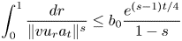 \begin{equation} \int_{0}^1\frac{dr}{\|vu_ra_t\|^{s}} \le b_0 \frac{e^{(s-1)t/4}}{1-s} \end{equation}
where  $vh= \operatorname {Ad}(h) (v)$ for all $h\in H$.
Remark A.2 It is worth noting that the symmetric interval  $[-1,1]$ was used in Lemma 5.6. We remark that this is necessary in the infinite volume setting; indeed the half interval $[0,1]$ may even be a null set for $\mu _y$ for some $y$; see (4.1) for the notation.
For a locally bounded function  $\psi$ on $Y$ and $t>0$, define
 \begin{equation} {\mathsf{A}}_t\psi (y)= \int_{0}^1 \psi (yu_ra_t)\,dr \quad\text{for $y\in Y$}. \end{equation}
Proposition A.4 Let  $1/3\le s<1$. There exists $t=t(s)>0$ such that for all $y\in Y$,
 \begin{equation} {\mathsf{A}}_t F_s(y) \le \tfrac{1}{2} F_s(y)+ c \, {\varepsilon}_X^{-4} \alpha_s^4 \operatorname{Vol}(Z)\end{equation}
where  $\alpha _s= (1-s)^{-1/(1-s)}$ and $c\ge 1$ is an absolute constant.
Proof. It suffices to show that  ${\mathsf {A}}_t f_s(y)\leq \tfrac {1}{2}f_s(y)+ \alpha _s^4 {\rm Vol}(Z)$.
Let  $b_0$ be as in (A.1), and let $t=t(s)$ be given by the equation
 \[ b_0 \frac{e^{(s-1)t /4}}{1-s} =1/2. \]
We compare  $f_s(yu_ra_t)$ and $f_s(y)$ for $r\in [0,1]$. Let $C_1\asymp e^{ t}$ be large enough so that $\|vh\|\leq C_1\|v\|$ for all $v\in i\frak {sl}_2(\mathbb {R})$ and all
 \[ h\in \{a_\tau u_r: | r|<1, |\tau|\leq t\}. \]
Let  $v\in I_Z(yu_ra_t)$ be so that $\|v\|< {\varepsilon }_X/C_1$. Then $\|va_{-t}u_{-r}\|\leq {\varepsilon }_X$; in particular, $va_{-t}u_{-r}\in I_Z(y)$.
In the following, if  $I_Z(\cdot )=\emptyset$, the sum is interpreted as to equal to ${\varepsilon }_X^{-s}$. In view of the above observation and the definition of $f_s$, we have
 \begin{align} f_s(yu_ra_t)&=\sum_{v\in I_Z(yu_ra_t)}\|v\|^{-s}\nonumber\\ &=\sum_{v\in I_Z(yu_ra_t), \|v\|< {\varepsilon}_X/C_1}\|v\|^{-s}+\sum_{v\in I_Z(yu_ra_t), \|v\|\geq {\varepsilon}_X/C_1}\|v\|^{-s}\nonumber\\ &\leq \sum_{v\in I_Z(y)}\|vu_ra_t\|^{-s}+\sum_{v\in I_Z(yu_ra_t), \|v\|\geq {\varepsilon}_X/C_1}\|v\|^{-s}. \end{align}
Moreover, note that  $\# I_Z(y)\ll {\varepsilon }_X^{-3} {\rm Vol}(Z)$ (see the proof of Lemma 8.13). Hence,
 \begin{equation} \sum_{\|v\|\geq {\varepsilon}_X/C_1}\|v\|^{-s}\ll C_1^s {\varepsilon}_X^{-4} {\rm Vol}(Z) \ll {\varepsilon}_X^{-4} e^{st} {\rm Vol}(Z). \end{equation}
 We now average (A.6) over  $[0,1]$. Then using (A.7) and (A.1) we get
 \[ {\mathsf{A}}_t f_s(y)\leq \tfrac{1}{2}f_s(y)+ O(e^{st} {\rm Vol}(Z)). \]
As  $(1-s)^{-1/(1-s)} \asymp e^{st/4}$, this proves (A.5).
Let  $m_Y$ be the $H$-invariant probability measure on $Y$.
$Y$.
Corollary A.8 We have
 \[ m_Y(F_s) \le c \, {\varepsilon}_X^{-4}\alpha_s^4 \operatorname{Vol}(Z) \]
where  $c\ge 1$ is an absolute constant.
Proof. Since  $m_Y$ is an $H$-invariant probability measure, $m_Y({\mathsf {A}}_t f_s)=m_Y(f_s)$. Hence the claim follows by integrating (A.5) with respect to $m_Y$.
Proof of Theorem 1.1 There exists  $\sigma >0$ such that for any $h\in B_H({\varepsilon }_X)$ and $y\in Y$, $F_s(y)\le \sigma F_s(yh)$ (cf. Lemma 9.10); $B_H({\varepsilon }_X)$ denotes the ${\varepsilon }_X$-ball centered at the identity in $H$.
$H$.
Hence, using Corollary A.8, we deduce
 \begin{align*} f_s(y) &\le F_s(y)\le \frac{\sigma\int_{B_H( {\varepsilon}_X)} F_s (yh) \,dm_Y(yh)}{m_Y(B(y, {\varepsilon}_X))}\\ &\le \frac{\sigma\cdot{m_Y(F_s)} }{m_Y(B(y, {\varepsilon}_X))} \ll \alpha_s^4 {\varepsilon}_X^{-7} \operatorname{Vol}(Y) \operatorname{Vol}(Z) \end{align*}
with an absolute implied constant. Since  $d(y, Z)^{-s}\le c_1 f_s(y)$ for an absolute constant $c_1\ge 1$ (see (10.4)), we have
 \begin{equation} d(y, Z)\gg \alpha_s^{-4/s} {\varepsilon}_X^{7/s}\operatorname{Vol}(Z)^{-1/s} \operatorname{Vol}(Y)^{-1/s}. \end{equation}
This shows Theorem 1.1(1). By Corollary A.8 and the Chebyshev inequality, we get
 \[ m_Y\{y\in Y: d(y, Z)\le {\varepsilon}\} \le m_Y\{y\in Y: F_s(y) \ge c_1^{-1} {\varepsilon}^{-s}\} \le c_1 m_Y(F_s) {\varepsilon}^s. \]
Therefore
 \begin{equation} m_Y\{y\in Y: d(y, Z)\le {\varepsilon}\} \le c_1 c {\varepsilon}^s {\varepsilon}_X^{-4}\alpha_s^4 \operatorname{Vol} (Z), \end{equation}
which implies Theorem 1.1(2).


 Open access