


Impact Statement
This manuscript highlights one of the first approaches for quantifying the uncertainty in deep learning-based surrogate modeling coupled with finite-element analysis, which is a rising area of research and interest given their potential to offset the computational cost of finite element methods alone.
1. Introduction
Mechanical deformation of elastic materials is greatly influenced by microscale features (such as grains, thermodynamical phases, inclusions) as well as geometric features (such as cracks, notches, voids, etc.) (Knott, Reference Knott1973; Wu et al., Reference Wu, MacEwen, Lloyd and Neale2004; Roters et al., Reference Roters, Eisenlohr, Hantcherli, Tjahjanto, Bieler and Raabe2010; Kalidindi, Reference Kalidindi2015; Karlson et al., Reference Karlson, Skulborstad, Madison, Polonsky, Jin, Jones, Sanborn, Kramer, Antoun and Lu2023) spanning multiple length scales. Numerical methods such as the finite element method (FEM) typically incorporate a physically motivated multi-scale representation of such geometries/features to properly resolve the effects they have across disparate length scales. Common examples of such methods include staggered solution schemes for coarse- and fine-scale meshes such as the Schwarz alternating method (Mota et al., Reference Mota, Tezaur and Phlipot2022) or the global–local generalized finite element method (GFEM-gl) (Duarte and Kim, Reference Duarte and Kim2008); material formulations that account for mechanical deformation through homogenized properties such as Miehe and Bayreuther (Reference Miehe and Bayreuther2007) and Geers et al. (Reference Geers, Kouznetsova and Brekelmans2010); variational multiscale (Liu and Marsden, Reference Liu and Marsden2018); and reduced order models (Ganapathysubramanian and Zabaras, Reference Ganapathysubramanian and Zabaras2004).
The computational efficiency of multi-scale approaches deteriorates as the complexity of the material model and/or the number of elements increases due to the expense of tasks such as the imposition of plasticity constraints and the numerical integration of auxiliary variables like damage at each quadrature point, which are typically performed at each time/continuation step of a simulation. Consequently, full simulations become untenable as the number of elements increase to the tens to hundreds of millions, even for today’s fastest computers (Balzani et al., Reference Balzani, Gandhi, Klawonn, Lanser, Rheinbach and Schröder2016; Budarapu et al., Reference Budarapu, Zhuang, Rabczuk and Bordas2019; Klawonn et al., Reference Klawonn, Lanser, Rheinbach and Uran2021).
Surrogate models have been developed as an alternative to finite element simulations of high-fidelity models by replacing the most computational expensive routines with approximations that are trained offline using data obtained from previous finite element analyses and/or experiments. Focusing on NN-based approaches, prior work in these types of models include approximations of constitutive and balance laws (Huang et al., Reference Huang, Fuhg, Weißenfels and Wriggers2020; Wu et al., Reference Wu, Nguyen, Kilingar and Noels2020; Aldakheel et al., Reference Aldakheel, Satari and Wriggers2021; Benabou, Reference Benabou2021; Wu and Noels, Reference Wu and Noels2022), homogenization schemes (Wang and Sun, Reference Wang and Sun2018; Wu et al., Reference Wu, Nguyen, Kilingar and Noels2020; Wu and Noels, Reference Wu and Noels2022), and methods that simplify or fully replace finite element analyses (Koeppe et al., Reference Koeppe, Bamer and Markert2018, Reference Koeppe, Bamer and Markert2019, Reference Koeppe, Bamer and Markert2020; Capuano and Rimoli, Reference Capuano and Rimoli2019; Im et al., Reference Im, Lee and Cho2021).
Illustrative examples of surrogate models used to approximate constitutive laws include approaches that predict stresses of history-dependent materials using variants of feed-forward networks (Huang et al., Reference Huang, Fuhg, Weißenfels and Wriggers2020), recurrent neural networks (RNNs) such as Long-Short Term Memory (LSTM) (Benabou, Reference Benabou2021), and the Gated Recurrent Unit (GRU) (Wu et al., Reference Wu, Nguyen, Kilingar and Noels2020; Wu and Noels, Reference Wu and Noels2022). Works such as Wang and Sun (Reference Wang and Sun2018), Wu et al. (Reference Wu, Nguyen, Kilingar and Noels2020), and Wu and Noels (Reference Wu and Noels2022) specifically focus on reducing the computational complexity of traditional multi-scale approaches such as $ {\mathrm{FE}}^2 $
by approximating the homogenized fields and properties thus eliminating the need to solve the full boundary-value problem for representative volume elements (RVEs). The authors in Aldakheel et al. (Reference Aldakheel, Satari and Wriggers2021) replace the costly numerical integration of an ordinary differential equation (ODE) for a phase-field variable that controls the stress degradation with a NN-based approximation. In Im et al. (Reference Im, Lee and Cho2021), the authors construct models that predict the full displacement, stress, or force fields for a given geometry such as a structural frame. In these cases, the surrogate fully replaces the need to run a finite element analysis for the given geometry and set of boundary conditions. In another example, a forcing term is trained to predict the corrections/errors on a coarse mesh for a given boundary-value problem solved on a refined mesh (Baiges et al., Reference Baiges, Codina, Castañar and Castillo2020). The authors achieved accurate predictions of the deformation for a cantilever beam bending problem using a coarsened mesh and a trained error correction term. In the approaches of Koeppe et al. (Reference Koeppe, Bamer and Markert2018, Reference Koeppe, Bamer and Markert2019, Reference Koeppe, Bamer and Markert2020) and Capuano and Rimoli (Reference Capuano and Rimoli2019), a machine-learned element is trained to predict a set of fields such as forces for only a single element. The full predictive power of such methods is demonstrated by predicting various quantities of interest in FEM simulations with meshed geometries composed of these machine-learned elements.
$ {\mathrm{FE}}^2 $
by approximating the homogenized fields and properties thus eliminating the need to solve the full boundary-value problem for representative volume elements (RVEs). The authors in Aldakheel et al. (Reference Aldakheel, Satari and Wriggers2021) replace the costly numerical integration of an ordinary differential equation (ODE) for a phase-field variable that controls the stress degradation with a NN-based approximation. In Im et al. (Reference Im, Lee and Cho2021), the authors construct models that predict the full displacement, stress, or force fields for a given geometry such as a structural frame. In these cases, the surrogate fully replaces the need to run a finite element analysis for the given geometry and set of boundary conditions. In another example, a forcing term is trained to predict the corrections/errors on a coarse mesh for a given boundary-value problem solved on a refined mesh (Baiges et al., Reference Baiges, Codina, Castañar and Castillo2020). The authors achieved accurate predictions of the deformation for a cantilever beam bending problem using a coarsened mesh and a trained error correction term. In the approaches of Koeppe et al. (Reference Koeppe, Bamer and Markert2018, Reference Koeppe, Bamer and Markert2019, Reference Koeppe, Bamer and Markert2020) and Capuano and Rimoli (Reference Capuano and Rimoli2019), a machine-learned element is trained to predict a set of fields such as forces for only a single element. The full predictive power of such methods is demonstrated by predicting various quantities of interest in FEM simulations with meshed geometries composed of these machine-learned elements.
The common assumption in the above approaches is that the surrogate model only makes predictions on inputs that are near the data it was trained on. Such limitations are discussed briefly in the concluding remarks of works such as Koeppe et al. (Reference Koeppe, Bamer and Markert2019), Wu et al. (Reference Wu, Nguyen, Kilingar and Noels2020), and Aldakheel et al. (Reference Aldakheel, Satari and Wriggers2021), but potential solutions are left as research directions for future work. The degree of uncertainty in these surrogate models’ predictions is crucial in determining whether such estimates represent an accurate and physically relevant approximation of the original finite element model. Prior work on uncertainty quantification in machine learning includes predictions of uncertainty due to noise (Yang et al., Reference Yang, Meng and Karniadakis2021), and predictions of distributions over possible solutions where training data is sparse or nonexistent (Zhu et al., Reference Zhu, Zabaras, Koutsourelakis and Perdikaris2019). Other similar applications are also highlighted in Zou et al. (Reference Zou, Meng, Psaros and Karniadakis2022). The uncertainty described in these works pertains to problems where physics-constrained NNs predict fields that satisfy some governing ordinary or partial differential equation subject to prescribed initial and/or boundary conditions. To the authors’ knowledge, uncertainty quantification for hybrid approaches that couple NNs with discretization methods such as FEM for simulating the deformation of solids has not been extensively studied to date.
In the current work, uncertainty estimates of predictions that surrogate models produce are constructed within the framework of a coupled FEM-NN approach similar to those of Koeppe et al. (Reference Koeppe, Bamer and Markert2018, Reference Koeppe, Bamer and Markert2019, Reference Koeppe, Bamer and Markert2020) and Capuano and Rimoli (Reference Capuano and Rimoli2019). In this approach, the machine-learned elements predict internal forces given displacements for a subregion of a full-scale geometry, while the rest of the meshed geometry contains elements whose internal forces are computed with the traditional evaluation of the stresses via the FEM. Ensembles of Bayesian neural networks (BNNs) (Fort et al., Reference Fort, Hu and Lakshminarayanan2019) are used to generate a diverse set of internal force predictions. A novel tolerance interval-inspired approach is introduced to account for uncertainty in the ensemble predictions. Ultimately, this approach is used to assess reliability of the NN predictions for a wide range of possible loading conditions. We believe the proposed method provides a powerful tool for quantifying the uncertainty of predictions for NN-based models when coupled with FEM.
The article is organized as follows: In Section 2, the theoretical background on FEM and NNs is presented. In Section 3, the training and uncertainty estimation procedures are discussed. In Section 4, the proposed procedure is highlighted for a three-element geometry with a single machine-learned surrogate element, and the results are discussed. Concluding remarks are presented in Section 5.
2. Theoretical background
2.1. Finite element formulation
Consider a spatially discretized domain in the current/deformed configuration at some specified time $ t $
(omitted on domains and fields for brevity) as
$ t $
(omitted on domains and fields for brevity) as $ \Omega $
composed of a set of finite elements
$ \Omega $
composed of a set of finite elements $ {\Omega}^e $
,
$ {\Omega}^e $
,
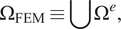 $$ {\Omega}_{\mathrm{FEM}}\equiv \cup {\Omega}^e, $$
and a contiguous segment of NN elements $ {\Omega}_{\mathrm{NN}}^e $
,
$ {\Omega}_{\mathrm{NN}}^e $
,
 $$ {\Omega}_{\mathrm{NN}}\equiv \cup {\Omega}_{\mathrm{NN}}^e, $$
with an imposed set of boundary conditions
 $$ {\displaystyle \begin{array}{cc}\boldsymbol{T}\hskip0.2em \boldsymbol{n}& =\overline{\boldsymbol{t}}\hskip0.35em \mathrm{o}\mathrm{n}\hskip0.35em \mathrm{\partial}{\Omega}_t\\ {}\boldsymbol{u}& =\overline{\boldsymbol{u}}\hskip0.35em \mathrm{o}\mathrm{n}\hskip0.35em \mathrm{\partial}{\Omega}_u\end{array}} $$
as shown in Figure 1. In the above equation, $ \boldsymbol{T} $
is the Cauchy stress tensor,
$ \boldsymbol{T} $
is the Cauchy stress tensor, $ \boldsymbol{n} $
is the outward-facing unit normal on
$ \boldsymbol{n} $
is the outward-facing unit normal on $ \mathrm{\partial \Omega } $
,
$ \mathrm{\partial \Omega } $
, $ \boldsymbol{u} $
is the displacement relative to a stress-free reference configuration, and
$ \boldsymbol{u} $
is the displacement relative to a stress-free reference configuration, and $ \overline{\boldsymbol{t}} $
and
$ \overline{\boldsymbol{t}} $
and $ \overline{\boldsymbol{u}} $
are the imposed set of boundary traction and displacement (respectively). Additionally, the superscript
$ \overline{\boldsymbol{u}} $
are the imposed set of boundary traction and displacement (respectively). Additionally, the superscript $ e $
signifies a unique element identifier.
$ e $
signifies a unique element identifier.
Figure 1. Discretized domain $ \Omega $
highlighting the NN element domain
$ \Omega $
highlighting the NN element domain $ {\Omega}_{\mathrm{NN}} $
(green) and finite element domain
$ {\Omega}_{\mathrm{NN}} $
(green) and finite element domain $ {\Omega}_{\mathrm{FEM}} $
.
$ {\Omega}_{\mathrm{FEM}} $
.
The spatially discretized Bubnov–Galerkin formulation for the balance of static forces for a given finite element $ {\Omega}^e $
is (Hughes, Reference Hughes2012)
$ {\Omega}^e $
is (Hughes, Reference Hughes2012)
 $$ [{\boldsymbol{F}}_{int}^e(\boldsymbol{u})]-[{\boldsymbol{F}}_{ext}^e]=[\mathbf{0}], $$
where the finite element internal and external forces are defined as
 $$ {\displaystyle \begin{array}{l}\left[{\boldsymbol{F}}^{e,\mathit{\operatorname{int}}}\right]={\int}_{\Omega^e}{\left[{\boldsymbol{B}}^e\right]}^T\hat{\boldsymbol{T}}\; dv\\ {}\left[{\boldsymbol{F}}^{e,\mathit{\operatorname{ext}}}\right]={\int}_{\partial {\Omega}^e\cap {\Gamma}_t}{\left[{\boldsymbol{N}}^e\right]}^T\overline{\boldsymbol{t}}\; da+{\int}_{\partial {\Omega}^e\setminus {\Gamma}_t}{\left[{\boldsymbol{N}}^e\right]}^T\boldsymbol{t}\; da\end{array}}. $$
In the above equation, $ \hat{\boldsymbol{T}} $
is the Cauchy stress ordered in Voigt notation, and
$ \hat{\boldsymbol{T}} $
is the Cauchy stress ordered in Voigt notation, and $ \left[{\boldsymbol{N}}^e\right] $
and
$ \left[{\boldsymbol{N}}^e\right] $
and $ \left[{\boldsymbol{B}}^e\right] $
are the traditional arrays of the finite element shape functions and their derivatives.
$ \left[{\boldsymbol{B}}^e\right] $
are the traditional arrays of the finite element shape functions and their derivatives.
Define the linearized strain $ \boldsymbol{\epsilon} $
as the symmetric material gradient of the displacement,
$ \boldsymbol{\epsilon} $
as the symmetric material gradient of the displacement,
 $$ \boldsymbol{\epsilon} =\frac{1}{2}\left[\frac{\partial \boldsymbol{u}}{\partial \boldsymbol{X}}+{\left(\frac{\partial \boldsymbol{u}}{\partial \boldsymbol{X}}\right.)}^T\right]. $$
Following the classical approach (Simo and Hughes, Reference Simo and Hughes1998), we admit an additive decomposition of the strain $ \boldsymbol{\epsilon} $
into an elastic and plastic contribution
$ \boldsymbol{\epsilon} $
into an elastic and plastic contribution $ {\boldsymbol{\epsilon}}^e $
and
$ {\boldsymbol{\epsilon}}^e $
and $ {\boldsymbol{\epsilon}}^p $
(respectively) at a given point in
$ {\boldsymbol{\epsilon}}^p $
(respectively) at a given point in $ {\Omega}_{\mathrm{FEM}} $
of the form
$ {\Omega}_{\mathrm{FEM}} $
of the form
 $$ \boldsymbol{\epsilon} ={\boldsymbol{\epsilon}}^e+{\boldsymbol{\epsilon}}^p. $$
The (linearized) Cauchy stress $ \boldsymbol{\sigma} $
(here we assume the linearized Cauchy stress
$ \boldsymbol{\sigma} $
(here we assume the linearized Cauchy stress $ \boldsymbol{\sigma} $
is equivalent to the Cauchy stress
$ \boldsymbol{\sigma} $
is equivalent to the Cauchy stress $ \boldsymbol{T} $
) is defined as
$ \boldsymbol{T} $
) is defined as
 $$ \boldsymbol{\sigma} =\mathrm{\mathbb{C}}\cdot {\boldsymbol{\epsilon}}^e, $$
where $ \mathrm{\mathbb{C}} $
is the classical fourth-order elasticity tensor. Plasticity is introduced through inequality constraint on the yield function
$ \mathrm{\mathbb{C}} $
is the classical fourth-order elasticity tensor. Plasticity is introduced through inequality constraint on the yield function $ f\left(\boldsymbol{\sigma}, h\right.) $
which takes the following form,
$ f\left(\boldsymbol{\sigma}, h\right.) $
which takes the following form,
 $$ f(\boldsymbol{\sigma}, h\operatorname{})=\phi (\boldsymbol{\sigma} \operatorname{})-({\sigma}_y+h({\boldsymbol{\epsilon}}^p))\le 0. $$
In equation (9), $ \phi \left(\boldsymbol{\sigma} \right.) $
is the effective stress which, here, is the von Mises criterion,
$ \phi \left(\boldsymbol{\sigma} \right.) $
is the effective stress which, here, is the von Mises criterion,
 $$ \phi \left(\boldsymbol{\sigma} \right.) =\sqrt{\frac{2}{3}\boldsymbol{S}\cdot \boldsymbol{S}}, $$
where $ \boldsymbol{S} $
is the deviatoric stress tensor
$ \boldsymbol{S} $
is the deviatoric stress tensor
 $$ \boldsymbol{S}=\boldsymbol{\sigma} -\frac{1}{3} tr\left(\boldsymbol{\sigma} \right.) \boldsymbol{I}. $$
Additionally, $ {\sigma}_y $
is the yield stress, and
$ {\sigma}_y $
is the yield stress, and $ h\left({\boldsymbol{\epsilon}}^p\right.) $
is the isotropic hardening, which is assumed to be a function of the plastic strain
$ h\left({\boldsymbol{\epsilon}}^p\right.) $
is the isotropic hardening, which is assumed to be a function of the plastic strain $ {\boldsymbol{\epsilon}}^p $
.
$ {\boldsymbol{\epsilon}}^p $
.
The plastic strain $ {\boldsymbol{\epsilon}}^p $
is defined assuming associative flow as
$ {\boldsymbol{\epsilon}}^p $
is defined assuming associative flow as
 $$ {\boldsymbol{\epsilon}}^p=\gamma \frac{\boldsymbol{S}}{\left\Vert \boldsymbol{S}\right\Vert }, $$
where $ \gamma $
is a nonnegative consistency parameter. The Kuhn–Tucker conditions are
$ \gamma $
is a nonnegative consistency parameter. The Kuhn–Tucker conditions are
 $$ \left\{\begin{array}{l}f\left(\boldsymbol{\sigma}, h\right.) \le 0\\ {}\gamma \ge 0\\ {}\gamma f\left(\boldsymbol{\sigma}, h\right.) =0\end{array}\right., $$
and the consistency condition is
 $$ \gamma \dot{f}\left(\boldsymbol{\sigma}, h\right.) =0. $$
Together, equations (9), (13), and (14) form the full set of plasticity constraints for loading/unloading. The plasticity constraint equations coupled with the constitutive equation in equation (8) provide a closed-form definition of the Cauchy stress needed to evaluate the internal forces in equation (5).
Akin to coupled FEM-NN methods proposed in Capuano and Rimoli (Reference Capuano and Rimoli2019) and Koeppe et al. (Reference Koeppe, Bamer and Markert2020), the internal force term for the NN elements $ {\Omega}_{\mathrm{NN}}^e $
is given by a regression tool such as a NN,
$ {\Omega}_{\mathrm{NN}}^e $
is given by a regression tool such as a NN,
 $$ [{\boldsymbol{F}}_{\mathrm{NN}}^{e,\mathrm{int}}]\equiv [\hskip0.35em {\boldsymbol{f}}_{\mathrm{NN}}({\boldsymbol{u}}^e,{\boldsymbol{w}}_{\mathrm{NN}},{\boldsymbol{b}}_{\mathrm{NN}})], $$
where $ {\boldsymbol{f}}_{\mathrm{NN}} $
is a nonlinear function of the element displacements
$ {\boldsymbol{f}}_{\mathrm{NN}} $
is a nonlinear function of the element displacements $ {\boldsymbol{u}}^e $
, NN weights
$ {\boldsymbol{u}}^e $
, NN weights $ {\boldsymbol{w}}_{\mathrm{NN}} $
and biases
$ {\boldsymbol{w}}_{\mathrm{NN}} $
and biases $ {\boldsymbol{b}}_{\mathrm{NN}} $
. The internal forces predicted by
$ {\boldsymbol{b}}_{\mathrm{NN}} $
. The internal forces predicted by $ {\boldsymbol{f}}_{\mathrm{NN}} $
are, in general, assumed to approximate the relation between the forces and displacements for the material occupying the NN elements. As such, the predicted forces given by
$ {\boldsymbol{f}}_{\mathrm{NN}} $
are, in general, assumed to approximate the relation between the forces and displacements for the material occupying the NN elements. As such, the predicted forces given by $ {\boldsymbol{f}}_{\mathrm{NN}} $
represent a mechanical response to physically imposed motion, and should thus be trained using a set of relevant forces/displacements.
$ {\boldsymbol{f}}_{\mathrm{NN}} $
represent a mechanical response to physically imposed motion, and should thus be trained using a set of relevant forces/displacements.
It is important to mention that the internal force in equation (15) depends on the reference frame used to express the displacements. Additionally, the internal force in equation (15) does not contain any history variables, and thus cannot predict processes that depend on loading history, such as inelastic cyclic loading. Treatment of the reliance of forces/displacements on their respective orientations relative to a fixed reference frame, as well as the dependence of the forces on the history of displacement in the context of FEM-NN approaches, is discussed in Capuano and Rimoli (Reference Capuano and Rimoli2019) and Koeppe et al. (Reference Koeppe, Bamer and Markert2020) (respectively), among other works. In the current context, we assume that the mechanical deformation does not incur large deformations and rotations on elements in the NN domain, and the initial configuration and orientations of the geometry do not change between each training data set and prediction. Additionally, all loads used for training, validation, and prediction are monotonic. These are limitations that simplify the training/prediction of forces in the NN domain. Proper treatment and modifications that account for dependence on reference frame and force/displacement history will be discussed in future work.
The NN element’s balance of forces takes the same form as equation (4), namely,
 $$ [{\boldsymbol{F}}_{\mathrm{NN}}^{e,\mathrm{int}}({\boldsymbol{u}}^e)]-[{\boldsymbol{F}}^{e,\mathrm{ext}}]=[\mathbf{0}]. $$
The set of element-wise internal and external forces are assembled across all elements in $ \Omega $
to form the full system of equations,
$ \Omega $
to form the full system of equations,
 $$ [{\boldsymbol{F}}^{int}(\boldsymbol{u})]-[{\boldsymbol{F}}^{ext}]=[\mathbf{0}], $$
where the global internal and external forces are defined as the element-wise assembly of their local counterparts (notated with the assembly operator $ \mathrm{A} $
acting on each element
$ \mathrm{A} $
acting on each element $ e $
), that is,
$ e $
), that is,
 $$ {\displaystyle \begin{array}{c}[{\boldsymbol{F}}^{int}(\boldsymbol{u})]=\underset{e}{\mathrm{A}}{\boldsymbol{F}}^{e,\mathrm{int}}(\boldsymbol{u})\\ {}[{\boldsymbol{F}}^{ext}]=\underset{e}{\mathrm{A}}{\boldsymbol{F}}^{e,\mathrm{ext}}\end{array}}. $$
The solution is the set of displacements $ \boldsymbol{u} $
that satisfies global balance of forces (equation (5)) given the set of boundary conditions in equation (3), a constitutive law governing the relation between the deformation/strains and the Cauchy stress, and an assumed function
$ \boldsymbol{u} $
that satisfies global balance of forces (equation (5)) given the set of boundary conditions in equation (3), a constitutive law governing the relation between the deformation/strains and the Cauchy stress, and an assumed function $ {\boldsymbol{f}}_{\mathrm{NN}} $
mapping displacements to forces in
$ {\boldsymbol{f}}_{\mathrm{NN}} $
mapping displacements to forces in $ {\Omega}_{\mathrm{NN}}^e $
. The full coupled FEM-NN procedure is shown in Algorithm 1.
$ {\Omega}_{\mathrm{NN}}^e $
. The full coupled FEM-NN procedure is shown in Algorithm 1.
The global internal force in equation (18) can be a nonlinear function of the displacements $ \boldsymbol{u} $
(for either/both the finite element and/or NN element domains). Therefore, obtaining a global displacement vector
$ \boldsymbol{u} $
(for either/both the finite element and/or NN element domains). Therefore, obtaining a global displacement vector $ \boldsymbol{u} $
that satisfies balance of forces across the entire domain
$ \boldsymbol{u} $
that satisfies balance of forces across the entire domain $ \Omega $
is typically obtained through iterative methods where each iteration predicts a trial set of displacements/forces to minimize a residual of the form
$ \Omega $
is typically obtained through iterative methods where each iteration predicts a trial set of displacements/forces to minimize a residual of the form
 $$ [\boldsymbol{R}(\boldsymbol{u})]=[{\boldsymbol{F}}^{int}(\boldsymbol{u})]-[{\boldsymbol{F}}^{ext}]. $$
Using numerical integration techniques to evaluate the integral for the internal forces in equation (5) for the traditional finite elements involves the evaluation of the Cauchy stresses at each quadrature point at each iteration. In general, this procedure can be computationally expensive when inelastic deformation takes place due to imposition of plasticity constraints, and in some cases, the evaluation of any state variables that are relevant. In contrast, the evaluation of the NN element internal forces simply involves the computation of $ {\boldsymbol{f}}_{\mathrm{NN}} $
at each of the element nodes for a given iteration. The lack of physical constraints and numerical solutions of additional variables needed to determine the Cauchy stress can make the evaluation of
$ {\boldsymbol{f}}_{\mathrm{NN}} $
at each of the element nodes for a given iteration. The lack of physical constraints and numerical solutions of additional variables needed to determine the Cauchy stress can make the evaluation of $ {\boldsymbol{f}}_{\mathrm{NN}} $
less computationally expensive at the cost of training a NN to predict a set of forces given a set of displacements.
$ {\boldsymbol{f}}_{\mathrm{NN}} $
less computationally expensive at the cost of training a NN to predict a set of forces given a set of displacements.
Algorithm 1. Coupled FEM-NN procedure
-
1: Initialize $ {t}_0 $
and
$ {\Omega}_{t_0} $
$ {t}_0 $
and
$ {\Omega}_{t_0} $
-
2: Set solver parameters
$ {\mathrm{iter}}_{\mathrm{max}} $
,
$ \mathrm{tol} $
$ \vartriangleright $
max nonlinear iterations and residual tolerance -
3: Set
$ i=1 $
-
4: while
$ i\le n\_\mathrm{steps} $
do ⊳Begin time loop -
5: Set time step
$ \Delta {t}_i $
-
6:
$ {t}_i\leftarrow {t}_{i-1}+\Delta {t}_i $
⊳Update current time -
7: Initialize trial displacements
$ {\boldsymbol{u}}_{t_i}^0 $
-
8: Initialize residual norm
$ {\left\Vert \left[\boldsymbol{R}\left({\boldsymbol{u}}_{t_i}^k\right)\right]\right\Vert}_2 $
to large number -
9: Set
$ k=0 $
-
10: Compute and assemble
$ \left[{\boldsymbol{F}}^{e,\mathit{\operatorname{ext}}}\right] $
-
11: while
$ k\le {\mathrm{iter}}_{\mathrm{max}} $
and
$ {\left\Vert \left[\boldsymbol{R}\left({\boldsymbol{u}}_{t_i}^k\right)\right]\right\Vert}_2\ge \mathrm{tol} $
do
$ \vartriangleright $
Iterate to obtain equilibrium displacements -
12: Compute and assemble
$ \left[{\boldsymbol{F}}_{\mathrm{NN}}^{e,\mathit{\operatorname{int}}}\left({\boldsymbol{u}}_{t_i}^k\right)\right] $
and
$ \left[{\boldsymbol{F}}_{\mathrm{FEM}}^{e,\mathit{\operatorname{int}}}\left({\boldsymbol{u}}_{t_i}^k\right)\right] $
-
13: Update residual
$ \left[\boldsymbol{R}\left({\boldsymbol{u}}_{t_i}^k\right)\right] $
-
14: Compute approximate tangent
-
15: Solve for
$ {\boldsymbol{u}}_{t_i}^{k+1} $
-
16:
$ k\leftarrow k+1 $
-
17: end while
-
18: Extract relevant QOIs
-
19:
$ i\leftarrow i+1 $
⊳Update simulation step -
20: end while


2.2. NN ensembles and Bayesian inference
NNs are a method for approximating nonlinear functional mappings between a set of inputs and a desired set of outputs (LeCun et al., Reference LeCun, Bengio and Hinton2015). NN models learn the desired functional mapping from a set of training results and subsequently use the learned function to predict the outputs for new/unseen inputs. NN models are able to establish that functional mapping by identifying an optimal set of features which are then regressed to the desired outputs. The typical transformation NNs use to obtain an output $ z $
from an
$ z $
from an $ n $
-dimensional input (assumed to be a vector)
$ n $
-dimensional input (assumed to be a vector) $ \boldsymbol{x}\in {\mathrm{\mathbb{R}}}^n $
is called a node (we term this an NN node hereafter to differentiate from nodes of a discretized mesh), and performs the following operation
$ \boldsymbol{x}\in {\mathrm{\mathbb{R}}}^n $
is called a node (we term this an NN node hereafter to differentiate from nodes of a discretized mesh), and performs the following operation
 $$ {z}_i\left({\boldsymbol{w}}_{\mathrm{NN},i},\boldsymbol{x},{b}_{\mathrm{NN},i}\right.) =f\left({\boldsymbol{w}}_{\mathrm{NN},i}^T\boldsymbol{x}+{b}_{\mathrm{NN},i}\right.), $$
where $ {\boldsymbol{w}}_{\mathrm{NN},i}\in {\mathrm{\mathbb{R}}}^n $
denotes the
$ {\boldsymbol{w}}_{\mathrm{NN},i}\in {\mathrm{\mathbb{R}}}^n $
denotes the $ i\mathrm{th} $
row of the weights that multiply the input. Similarly,
$ i\mathrm{th} $
row of the weights that multiply the input. Similarly, $ {b}_{\mathrm{NN},i} $
is the
$ {b}_{\mathrm{NN},i} $
is the $ i\mathrm{th} $
bias added to the resultant operation and
$ i\mathrm{th} $
bias added to the resultant operation and $ f\left(\right.) $
is a nonlinear activation function applied element-wise to its arguments.
$ f\left(\right.) $
is a nonlinear activation function applied element-wise to its arguments.
Feed forward neural networks (FFNN) sequentially stack layers to transform the inputs into the desired outputs, as illustrated in Figure 2. The number of nodes in a layer as well as the number of layers can be tuned for the specific task at hand. The values of the weights and biases of each layer are obtained by minimizing a loss function that quantifies the discrepancy between the values predicted by the model (i. e., the FFNN) and the known values of the training set. The minimization process is typically stopped when the value of the loss function reaches a pre-determined threshold. FFNNs are a very versatile and accurate surrogate model-building technique that have shown great success in a wide variety of applications and fields (Wang et al., Reference Wang, He and Liu2018; Wenyou and Chang, Reference Wenyou and Chang2020; Zhang and Mohr, Reference Zhang and Mohr2020; Muhammad et al., Reference Muhammad, Brahme, Ibragimova, Kang and Inal2021).
Figure 2. Schematic representation of a feed-forward network with two layers and scalar inputs/outputs.
BNNs have been widely studied for characterizing both aleatoric and epistemic uncertainties (Gal and Ghahramani, Reference Gal and Ghahramani2015; Sargsyan et al., Reference Sargsyan, Najm and Ghanem2015; Kendall and Gal, Reference Kendall and Gal2017; Knoblauch et al., Reference Knoblauch, Jewson and Damoulas2019). BNNs leverage the concept of Bayesian inference to sample from an assumed posterior distribution given some prior knowledge. Variational Bayesian inference (VBI) (Blundell et al., Reference Blundell, Cornebise, Kavukcuoglu and Wierstra2015) is a common approach used to train BNNs. Rather than attempting to sample from the true posterior, which is a computationally intractable problem, VBI assumes a distribution on the weights $ q(\boldsymbol{w}|\theta ) $
where
$ q(\boldsymbol{w}|\theta ) $
where $ \theta $
is the collection of hyperparameters associated with the assumed distribution. The weights are thus sampled from the distribution
$ \theta $
is the collection of hyperparameters associated with the assumed distribution. The weights are thus sampled from the distribution $ q $
. The hyperparameters
$ q $
. The hyperparameters $ \theta $
are optimized such that they minimize the variational free energy (also termed expected lower bounds, or ELBO) of the form
$ \theta $
are optimized such that they minimize the variational free energy (also termed expected lower bounds, or ELBO) of the form
where $ P(\boldsymbol{w}) $
is an assumed prior,
$ P(\boldsymbol{w}) $
is an assumed prior, $ \mathrm{KL}\left(\cdot \right.) $
is the Kullback–Leibler divergence, and
$ \mathrm{KL}\left(\cdot \right.) $
is the Kullback–Leibler divergence, and $ \mathcal{D} $
is the training data set. The first term in equation (21) signifies some measure of the distance between the assumed prior
$ \mathcal{D} $
is the training data set. The first term in equation (21) signifies some measure of the distance between the assumed prior $ P(\boldsymbol{w}) $
and the approximate posterior
$ P(\boldsymbol{w}) $
and the approximate posterior $ q(\boldsymbol{w}|\theta ) $
, which is assumed to always be positive or zero. The last term in equation (21) is a data-dependent likelihood term. The above equation poses an optimization of the approximate posterior
$ q(\boldsymbol{w}|\theta ) $
, which is assumed to always be positive or zero. The last term in equation (21) is a data-dependent likelihood term. The above equation poses an optimization of the approximate posterior $ q $
, with the aim of capturing information about the true posterior based only on knowledge of the assumed prior and the given data. In practice, an approximation of the variational free energy in equation (21) is used to train a BNN. This procedure is explained in Blundell et al. (Reference Blundell, Cornebise, Kavukcuoglu and Wierstra2015).
$ q $
, with the aim of capturing information about the true posterior based only on knowledge of the assumed prior and the given data. In practice, an approximation of the variational free energy in equation (21) is used to train a BNN. This procedure is explained in Blundell et al. (Reference Blundell, Cornebise, Kavukcuoglu and Wierstra2015).
The optimization process described above will yield a set of NN parameters that minimize the variational free energy in equation (21). The predictions of an optimized NN generally incur some amount of error. In the context of the FEM-NN approach highlighted in Section 2.1, the replacement of an internal force governed by local stresses that precisely satisfy the constitutive relation in equation (8) and plasticity constraints of equations (9), (13), and (14) with an approximation can commonly lead to a set of global displacements that satisfy the balance of forces in $ \Omega $
. Nevertheless, the approximation can deviate (sometimes significantly) from the true/expected deformation of the body under a given set of boundary conditions. This source of error is epistemic in nature, as it pertains to a lack of knowledge about single-valued (but uncertain) errors from numerous factors such as a finite amount of training data, an assumed form of the NN architecture and loss function, and an optimization of NN weights/biases that is a single realization from an inherently stochastic procedure.
$ \Omega $
. Nevertheless, the approximation can deviate (sometimes significantly) from the true/expected deformation of the body under a given set of boundary conditions. This source of error is epistemic in nature, as it pertains to a lack of knowledge about single-valued (but uncertain) errors from numerous factors such as a finite amount of training data, an assumed form of the NN architecture and loss function, and an optimization of NN weights/biases that is a single realization from an inherently stochastic procedure.
Among the various methods used to quantify and/or control epistemic uncertainty in machine-learning, the concept of NN ensembles (Fort et al., Reference Fort, Hu and Lakshminarayanan2019) is particularly relevant for this work. NN ensembles leverage multiple trained NNs termed “base learners.” Common ensembling strategies are randomized-based approaches that concurrently train multiple NNs on the same base data set such as bagging/bootstrapping (Lakshminarayanan et al., Reference Lakshminarayanan, Pritzel and Blundell2017), as well as other sequential training methods such as boosting and stacking (Yao et al., Reference Yao, Vehtari, Simpson and Gelman2018). The use of NN ensembles has been shown to substantially improve the quality of predictions, typically by enhancing diversity in those predictions thus reducing overall bias (Lakshminarayanan et al., Reference Lakshminarayanan, Pritzel and Blundell2017; Fort et al., Reference Fort, Hu and Lakshminarayanan2019; Hüllermeier and Waegeman, Reference Hüllermeier and Waegeman2021). In this work, ensembles are trained concurrently (as is done with traditional bagging approaches). Uncertainty estimates are obtained by bootstrap-sampling from the ensemble multiple times to obtain a distribution of predictions. This procedure is described in Section 3.
3. Uncertainty estimation of coupled FEM-NN approaches using ensembles
3.1. Generation of training and validation data
The training and validation data should encompass the sets of input displacements and output forces relevant for a given set of boundary-value problems. In the current context, the inputs and outputs are sampled in $ {\Omega}_{\mathrm{NN}} $
for a set of relevant boundary conditions. We define these boundary conditions
$ {\Omega}_{\mathrm{NN}} $
for a set of relevant boundary conditions. We define these boundary conditions $ \mathcal{B} $
in what is termed the primary space,
$ \mathcal{B} $
in what is termed the primary space, $ \mathrm{\mathbb{P}}\subset {\mathrm{\mathbb{R}}}^N $
, where
$ \mathrm{\mathbb{P}}\subset {\mathrm{\mathbb{R}}}^N $
, where $ N $
corresponds to the dimension of an assumed parameterization of the boundary conditions.
$ N $
corresponds to the dimension of an assumed parameterization of the boundary conditions.
For each boundary condition $ b\in \mathcal{B} $
, there exists a set of “exact” (i.
e., not approximated by surrogates) displacements
$ b\in \mathcal{B} $
, there exists a set of “exact” (i.
e., not approximated by surrogates) displacements $ {\boldsymbol{u}}_b $
that satisfy equilibrium in
$ {\boldsymbol{u}}_b $
that satisfy equilibrium in $ {\Omega}_{\mathrm{NN}} $
. Typically, these displacements are determined through a traditional finite element simulation. The “exact” internal forces associated with the displacements
$ {\Omega}_{\mathrm{NN}} $
. Typically, these displacements are determined through a traditional finite element simulation. The “exact” internal forces associated with the displacements $ {\boldsymbol{u}}_b $
in the elements occupying
$ {\boldsymbol{u}}_b $
in the elements occupying $ {\Omega}_{\mathrm{NN}} $
are simply computed using an assumed constitutive law that is a function of the displacements (through its gradient), such as the one shown in equation (8). The combined set of resulting element-level displacements
$ {\Omega}_{\mathrm{NN}} $
are simply computed using an assumed constitutive law that is a function of the displacements (through its gradient), such as the one shown in equation (8). The combined set of resulting element-level displacements $ {\boldsymbol{D}}_{u_b} $
and forces
$ {\boldsymbol{D}}_{u_b} $
and forces $ {\boldsymbol{D}}_{f_b} $
in
$ {\boldsymbol{D}}_{f_b} $
in $ {\Omega}_{\mathrm{NN}} $
are
$ {\Omega}_{\mathrm{NN}} $
are $ M $
-dimensional vectors defined in the secondary displacement space and secondary force space,
$ M $
-dimensional vectors defined in the secondary displacement space and secondary force space, $ {\unicode{x1D54A}}_u\subset {\mathrm{\mathbb{R}}}^M $
and
$ {\unicode{x1D54A}}_u\subset {\mathrm{\mathbb{R}}}^M $
and $ {\unicode{x1D54A}}_f\subset {\mathrm{\mathbb{R}}}^M $
, respectively. The combined sets of displacements and forces for all boundary conditions in
$ {\unicode{x1D54A}}_f\subset {\mathrm{\mathbb{R}}}^M $
, respectively. The combined sets of displacements and forces for all boundary conditions in $ \mathcal{B} $
are denoted
$ \mathcal{B} $
are denoted $ {\mathcal{D}}_u $
and
$ {\mathcal{D}}_u $
and $ {\mathcal{D}}_f $
(respectively).
$ {\mathcal{D}}_f $
(respectively).
In general, dimensionality reduction via methods such as principal component analysis (PCA) (Joliffe and Morgan, Reference Joliffe and Morgan1992) can be used to sample relevant boundary conditions in a reduced primary space $ {\mathrm{\mathbb{P}}}_r\subset {\mathrm{\mathbb{R}}}^n $
(where
$ {\mathrm{\mathbb{P}}}_r\subset {\mathrm{\mathbb{R}}}^n $
(where $ n<N $
), as well as generate training data in a reduced secondary input space
$ n<N $
), as well as generate training data in a reduced secondary input space $ {\unicode{x1D54A}}_{ur}\in {\mathrm{\mathbb{R}}}^m $
(where
$ {\unicode{x1D54A}}_{ur}\in {\mathrm{\mathbb{R}}}^m $
(where $ m<M $
). In the current setting, we assume dimensionality reduction is only performed on the secondary input space. We define the linear mapping between secondary and reduced secondary spaces obtained through PCA as
$ m<M $
). In the current setting, we assume dimensionality reduction is only performed on the secondary input space. We define the linear mapping between secondary and reduced secondary spaces obtained through PCA as $ {\boldsymbol{\varphi}}_{ur}:{\unicode{x1D54A}}_u\mapsto {\unicode{x1D54A}}_{ur} $
. The full input data set of all displacements in its reduced space is denoted
$ {\boldsymbol{\varphi}}_{ur}:{\unicode{x1D54A}}_u\mapsto {\unicode{x1D54A}}_{ur} $
. The full input data set of all displacements in its reduced space is denoted $ {\mathcal{D}}_{ur} $
.
$ {\mathcal{D}}_{ur} $
.
Once the full training and validation set are established, the displacements and forces are each scaled by their standard deviation and normalized to values between $ -1 $
and
$ -1 $
and $ 1 $
, that is,
$ 1 $
, that is,
 $$ \left\{\begin{array}{l}{\hat{D}}_{u_b}^i=\frac{{\overset{\sim }{D}}_{u_b}^i}{max\mid {\overset{\sim }{\boldsymbol{D}}}_u\mid },\hskip0.55em {\overset{\sim }{D}}_{u_b}^i=\frac{D_{u_b}^i}{\sigma \left({\boldsymbol{D}}_u^i\right)}\\ {}{\hat{D}}_{f_b}^i=\frac{{\overset{\sim }{D}}_{f_b}^i}{max\mid {\overset{\sim }{\boldsymbol{D}}}_f\mid },\hskip0.55em {\overset{\sim }{D}}_{f_b}^i=\frac{D_{f_b}^i}{\sigma \left({\boldsymbol{D}}_f^i\right.)}\end{array}\right.. $$
In the above equation, $ {\boldsymbol{D}}_u $
and
$ {\boldsymbol{D}}_u $
and $ {\boldsymbol{D}}_f $
are the full set of displacements
$ {\boldsymbol{D}}_f $
are the full set of displacements $ {\mathcal{D}}_u $
and forces
$ {\mathcal{D}}_u $
and forces $ {\mathcal{D}}_f $
(respectively) in matrix form. Additionally,
$ {\mathcal{D}}_f $
(respectively) in matrix form. Additionally, $ {\hat{D}}_{u_b}^i $
and
$ {\hat{D}}_{u_b}^i $
and $ {\hat{D}}_{f_b}^i $
are the scaled data for the
$ {\hat{D}}_{f_b}^i $
are the scaled data for the $ i\mathrm{th} $
component/feature of the
$ i\mathrm{th} $
component/feature of the $ b\mathrm{th} $
set of displacements and forces. Lastly,
$ b\mathrm{th} $
set of displacements and forces. Lastly, $ \sigma ({\boldsymbol{D}}_u^i) $
and
$ \sigma ({\boldsymbol{D}}_u^i) $
and $ \sigma ({\boldsymbol{D}}_f^i) $
are the standard deviations of the full displacement and force data sets for the
$ \sigma ({\boldsymbol{D}}_f^i) $
are the standard deviations of the full displacement and force data sets for the $ i\mathrm{th} $
component. Note that the standard deviations are computed only for the training data, though the scaling transformations are applied to both training and validation data. The NNs are subsequently trained
$ i\mathrm{th} $
component. Note that the standard deviations are computed only for the training data, though the scaling transformations are applied to both training and validation data. The NNs are subsequently trained $ {n}_e $
times to obtain multiple sets of optimal hyperparameters. The combined set of
$ {n}_e $
times to obtain multiple sets of optimal hyperparameters. The combined set of $ {n}_e $
NNs forms the ensemble used to make predictions. The full training procedure is shown in Algorithm 2.
$ {n}_e $
NNs forms the ensemble used to make predictions. The full training procedure is shown in Algorithm 2.
Algorithm 2. Training procedure
-
1: Generate set of relevant boundary conditions
$ \mathcal{B}\in \mathrm{\mathbb{P}} $
-
2: for
$ b\in \mathcal{B} $
do ⊳loop through relevant boundary conditions -
3: Compute displacements/forces
$ {\boldsymbol{D}}_{u_b} $
and
$ {\boldsymbol{D}}_{f_b} $
in secondary space
$ \unicode{x1D54A} $
⊳via FEM -
4: end for
-
5: Compute displacement mapping to reduced secondary space
$ {\unicode{x1D54A}}_{ur} $
-
6: Construct reduced training/validation input displacement data set
$ {\mathcal{D}}_{ur}\in {\unicode{x1D54A}}_{ur} $
-
7: for
$ b\in \mathcal{B} $
do -
8: Compute actual input displacement data
$ {\boldsymbol{D}}_{u_b}={\varphi}_{ur}^{-1}\left({\boldsymbol{D}}_{ur_b}\right) $
-
9: Compute output forces
$ {\boldsymbol{D}}_{f_b} $
-
10: end for
-
11: split full data sets
$ {\mathcal{D}}_u $
and
$ {\mathcal{D}}_b $
to training/validation
$ \left\{{\boldsymbol{D}}_{u,t},{\boldsymbol{D}}_{u,v}\right\} $
and
$ \left\{{\boldsymbol{D}}_{f,t},{\boldsymbol{D}}_{f,v}\right\} $
-
12: apply feature scaling to data sets
-
13: for
$ n\in \mathrm{range}\left({n}_e\right) $
do ⊳ loop through total number of NNs for the ensemble -
14: Randomly initialize weights
$ {\boldsymbol{w}}_{\mathrm{NN}}^n $
and biases
$ {\boldsymbol{b}}_{\mathrm{NN}}^n $
by sampling prior distribution -
15: Find optimal posteriors
$ {\boldsymbol{w}}_{\mathrm{NN}}^n\sim {\boldsymbol{q}}_w^n\left({\theta}_w^n\right) $
and
$ {\boldsymbol{b}}_{\mathrm{NN}}^n\sim {\boldsymbol{q}}_b^n\left({\theta}_b^n\right) $
⊳Using VBI -
16: end for


As an illustrative example of the procedure described above, consider a simple two-element cantilever beam embedded in two-dimensional space $ {\mathrm{\mathbb{R}}}^2 $
, as shown in Figure 3. The left end that has an applied load can be parameterized by variations in both the horizontal and vertical directions, therefore
$ {\mathrm{\mathbb{R}}}^2 $
, as shown in Figure 3. The left end that has an applied load can be parameterized by variations in both the horizontal and vertical directions, therefore $ N=2 $
. The set
$ N=2 $
. The set $ \mathcal{B} $
consists of variations of the applied load in the parameterized two-dimensional space, shown as the red points on the top plot in Figure 3. The NN-element has two independent degrees of freedom for its displacement and force on the left node, therefore
$ \mathcal{B} $
consists of variations of the applied load in the parameterized two-dimensional space, shown as the red points on the top plot in Figure 3. The NN-element has two independent degrees of freedom for its displacement and force on the left node, therefore $ M=2 $
. The element-level displacements
$ M=2 $
. The element-level displacements $ {\boldsymbol{D}}_{u_b} $
corresponding to the applied loads in primary space are shown as blue circles in the secondary space plot in Figure 3. Note that the force on the right node of the NN-element is always equal and opposite to that of the left node, and thus does not have independent degrees of freedom. For simplicity, the training and validation input data can be constructed as a grid of displacements in the reduced secondary space such that they span the original data
$ {\boldsymbol{D}}_{u_b} $
corresponding to the applied loads in primary space are shown as blue circles in the secondary space plot in Figure 3. Note that the force on the right node of the NN-element is always equal and opposite to that of the left node, and thus does not have independent degrees of freedom. For simplicity, the training and validation input data can be constructed as a grid of displacements in the reduced secondary space such that they span the original data $ {\boldsymbol{D}}_{u_b} $
, as schematically shown in Figure 3. In this setting, an interpolative prediction occurs when the input displacements lie within the grid, whereas extrapolative predictions encompass all the input space not spanned by the grid. For this problem, dimensionality reduction is not strictly needed since both primary and secondary spaces are two-dimensional.
$ {\boldsymbol{D}}_{u_b} $
, as schematically shown in Figure 3. In this setting, an interpolative prediction occurs when the input displacements lie within the grid, whereas extrapolative predictions encompass all the input space not spanned by the grid. For this problem, dimensionality reduction is not strictly needed since both primary and secondary spaces are two-dimensional.
Figure 3. Schematic of sampled boundary conditions in primary space $ \mathrm{\mathbb{P}} $
(top) and the corresponding displacements used to inform training/validation in secondary space
$ \mathrm{\mathbb{P}} $
(top) and the corresponding displacements used to inform training/validation in secondary space $ \unicode{x1D54A} $
(bottom). The circles attached to either side of the beam are the nodes associated with the degrees of freedom of this element. The red and blue arrows on the left diagrams correspond to the red and blue points on the right plots.
$ \unicode{x1D54A} $
(bottom). The circles attached to either side of the beam are the nodes associated with the degrees of freedom of this element. The red and blue arrows on the left diagrams correspond to the red and blue points on the right plots.
3.2. Uncertainty estimation procedure
For a given ensemble $ m $
of a load case
$ m $
of a load case $ T\in \mathcal{T} $
(with index
$ T\in \mathcal{T} $
(with index $ \tau $
), we define a statistical tolerance interval (Hahn and Meeker, Reference Hahn and Meeker1991) inspired uncertainty scaling factor
$ \tau $
), we define a statistical tolerance interval (Hahn and Meeker, Reference Hahn and Meeker1991) inspired uncertainty scaling factor $ {F}_{\tau, m} $
of the ensemble’s standard deviation
$ {F}_{\tau, m} $
of the ensemble’s standard deviation $ {\sigma}_{\tau, m} $
such that the true value of the QoI (obtained via FEM) denoted
$ {\sigma}_{\tau, m} $
such that the true value of the QoI (obtained via FEM) denoted $ {f}_{\tau, m}^{\mathrm{FEM}} $
is
$ {f}_{\tau, m}^{\mathrm{FEM}} $
is $ \pm {F}_{\tau, m}{\sigma}_{\tau, m} $
from the predicted mean
$ \pm {F}_{\tau, m}{\sigma}_{\tau, m} $
from the predicted mean $ {\mu}_{\tau, m} $
. With this requirement, the uncertainty scaling factor
$ {\mu}_{\tau, m} $
. With this requirement, the uncertainty scaling factor $ F $
can be expressed as
$ F $
can be expressed as
 $$ {F}_{\tau, m}=\frac{e_{\tau, m}}{\sigma_{\tau, m}}, $$
where the mean bias (absolute error of the mean prediction) is defined as $ {e}_{\tau, m}=\mid {f}_{\tau, m}^{\mathrm{FEM}}-{\mu}_{\tau, m}\mid $
. Based on the form of equation (23),
$ {e}_{\tau, m}=\mid {f}_{\tau, m}^{\mathrm{FEM}}-{\mu}_{\tau, m}\mid $
. Based on the form of equation (23), $ F $
can be interpreted as a metric of bias-to-variance ratio for a set of NN predictions. High values of
$ F $
can be interpreted as a metric of bias-to-variance ratio for a set of NN predictions. High values of $ F $
indicate that the subensemble predictions have a high mean bias and/or low standard deviation (and variance), whereas lower values of
$ F $
indicate that the subensemble predictions have a high mean bias and/or low standard deviation (and variance), whereas lower values of $ F $
indicate a low mean bias and/or high standard deviation.
$ F $
indicate a low mean bias and/or high standard deviation.
To account for the load-dependent variation in the uncertainty scaling factor $ F $
, a selected set of test/trial boundary conditions
$ F $
, a selected set of test/trial boundary conditions $ \mathcal{T} $
are constructed and sampled in primary space
$ \mathcal{T} $
are constructed and sampled in primary space $ \mathrm{\mathbb{P}} $
. For each boundary condition instance, the full boundary-value problem is solved via the FEM-NN method highlighted in Algorithm 1, and the predictions for each quantity of interest (QoI) are extracted at equilibrium. In this prediction process, each NN of the ensemble produces a different output due to the stochastic nature of training these networks via randomly initialized weights/biases, back-propagation (e.
g., using stochastic gradient descent), and the computation of an approximate variational free energy obtained via random sampling. The NN ensemble will thus produce a set of
$ \mathrm{\mathbb{P}} $
. For each boundary condition instance, the full boundary-value problem is solved via the FEM-NN method highlighted in Algorithm 1, and the predictions for each quantity of interest (QoI) are extracted at equilibrium. In this prediction process, each NN of the ensemble produces a different output due to the stochastic nature of training these networks via randomly initialized weights/biases, back-propagation (e.
g., using stochastic gradient descent), and the computation of an approximate variational free energy obtained via random sampling. The NN ensemble will thus produce a set of $ {n}_e $
predictions for a given test/trial case.
$ {n}_e $
predictions for a given test/trial case.
In practice, producing an ensemble-averaged prediction can be prohibitively expensive, as it requires the evaluation of $ {n}_e $
NNs for a given load/boundary condition. A subensemble of
$ {n}_e $
NNs for a given load/boundary condition. A subensemble of $ {n}_{ss} $
BNNs can be selected via random sampling to reduce the computational cost of the ensemble-averaged predictions. The number of NNs
$ {n}_{ss} $
BNNs can be selected via random sampling to reduce the computational cost of the ensemble-averaged predictions. The number of NNs $ {n}_{ss} $
that the subensembles contain is typically selected to optimize the cost of making predictions in a typical application setting. For instance, large models involving complicated discretized geometries may require smaller subensembles to maintain reasonable computational efficiency.
$ {n}_{ss} $
that the subensembles contain is typically selected to optimize the cost of making predictions in a typical application setting. For instance, large models involving complicated discretized geometries may require smaller subensembles to maintain reasonable computational efficiency.
To estimate uncertainty due to variations in subensemble predictions, we generate $ {n}_{se} $
unique combinations of subensembles, each composed of
$ {n}_{se} $
unique combinations of subensembles, each composed of $ {n}_{ss} $
BNNs. Each prediction of a given load case will have a scaling factor
$ {n}_{ss} $
BNNs. Each prediction of a given load case will have a scaling factor $ F $
based on its mean bias and standard deviation, as illustrated in Figure 4. With this set of information, each test case will have a distribution of
$ F $
based on its mean bias and standard deviation, as illustrated in Figure 4. With this set of information, each test case will have a distribution of $ F $
values, with the lowest ones representing the subset of NNs that are most optimal (i.
e., lowest mean bias and/or highest standard deviation). The uncertainty estimation calibration procedure described here is highlighted in Algorithm 3. Note that the prediction of a given BNN statistically varies, due to the uncertain nature of sampling from an approximate posterior. Therefore, this scaling factor
$ F $
values, with the lowest ones representing the subset of NNs that are most optimal (i.
e., lowest mean bias and/or highest standard deviation). The uncertainty estimation calibration procedure described here is highlighted in Algorithm 3. Note that the prediction of a given BNN statistically varies, due to the uncertain nature of sampling from an approximate posterior. Therefore, this scaling factor $ F $
accounts both for uncertainty between each BNN prediction as well as the uncertainty within a single BNN.
$ F $
accounts both for uncertainty between each BNN prediction as well as the uncertainty within a single BNN.
Algorithm 3. Uncertainty estimation procedure
-
1: Generate set of test loading conditions
$ \mathcal{T}\in \mathrm{\mathbb{P}} $
-
2:
$ \tau \leftarrow 0 $
⊳ Initialize test boundary condition counter -
3: for
$ T\in \mathcal{T} $
do -
4: Compute “exact” QoIs for BCs associated with
$ T $
⊳via high-fidelity FEM simulation -
5: for
$ n\in \mathrm{range}\left({n}_e\right) $
do -
6: Run FEM-NN simulations using
$ {\boldsymbol{w}}_{\mathrm{NN}}^n $
and
$ {\boldsymbol{b}}_{\mathrm{NN}}^n $
to compute internal forces
$ {F}_{\mathit{\operatorname{int}}, NN}^e $
-
7: if run succeeds then
-
8: Save QoIs
-
9: end if
-
10: end if
-
11: for
$ m\in \mathrm{range}\left({n}_{se}\right) $
do -
12: Randomly select
$ {n}_{ss} $
subsamples of QoIs from successful runs -
13: Compute mean bias
$ {e}_{\tau, m} $
and standard deviation
$ {\sigma}_{\tau, m} $
of QoIs -
14: Compute ensemble’s uncertainty scaling factor
$ {F}_{\tau, m}={e}_{\tau, m}/{\sigma}_{\tau, m} $
-
15: end for
-
16:
$ \tau \leftarrow \tau +1 $
⊳ Increment test boundary condition counter -
17: end for


Figure 4. Extraction of uncertainty for three sampled neural network subensembles for two sampled load cases with $ {n}_e=20 $
and
$ {n}_e=20 $
and $ {n}_{ss}=5 $
.
$ {n}_{ss}=5 $
.
3.3. Calibration and reliability of uncertainty estimates
In the current setting, we assume $ {n}_e=20 $
is a representative number of total NNs that is sufficient to capture reasonable diversity in predictions. Moreover,
$ {n}_e=20 $
is a representative number of total NNs that is sufficient to capture reasonable diversity in predictions. Moreover, $ {n}_{ss}=5 $
is chosen as a reasonable size for a subensemble that is relatively affordable for our applications. Lastly, the number of subensembles where we compute an uncertainty scaling factor is
$ {n}_{ss}=5 $
is chosen as a reasonable size for a subensemble that is relatively affordable for our applications. Lastly, the number of subensembles where we compute an uncertainty scaling factor is $ {n}_{se}=100 $
. Therefore, for each test point
$ {n}_{se}=100 $
. Therefore, for each test point $ T\in \mathcal{T} $
, there exist
$ T\in \mathcal{T} $
, there exist $ 100 $
values of
$ 100 $
values of $ F $
, corresponding to the
$ F $
, corresponding to the $ 100 $
different combinations of ensemble prediction biases/variances. The subensembles are randomly chosen (with a fixed random seed for reproducibility) from the
$ 100 $
different combinations of ensemble prediction biases/variances. The subensembles are randomly chosen (with a fixed random seed for reproducibility) from the $ {n}_e=20 $
ensembles such that each combination is unique.
$ {n}_e=20 $
ensembles such that each combination is unique.
The uppertail of the distribution of $ 100\ F $
values is a useful metric of the predictive uncertainty for this problem, since the highest values of
$ 100\ F $
values is a useful metric of the predictive uncertainty for this problem, since the highest values of $ F $
indicate the least reliable predictions (i.
e., highest bias and/or lowest variance) generated by the subensembles for a given load. More specifically, we assume that the
$ F $
indicate the least reliable predictions (i.
e., highest bias and/or lowest variance) generated by the subensembles for a given load. More specifically, we assume that the $ {95}^{\mathrm{th}} $
-percentile of
$ {95}^{\mathrm{th}} $
-percentile of $ F $
(for short will be notated
$ F $
(for short will be notated $ {F}^{95} $
) for a given test point
$ {F}^{95} $
) for a given test point $ T $
is sufficient to provide conservative estimates of the higher-end of bias/variance seen in the predictions while excluding outliers that detract from the primary trends. Note that this selection of an upper-bound is a heuristic parameter that is problem-dependent, and should be fine-tuned based on the observed distribution of
$ T $
is sufficient to provide conservative estimates of the higher-end of bias/variance seen in the predictions while excluding outliers that detract from the primary trends. Note that this selection of an upper-bound is a heuristic parameter that is problem-dependent, and should be fine-tuned based on the observed distribution of $ F $
values.
$ F $
values.
Since $ F $
varies spatially across the primary space
$ F $
varies spatially across the primary space $ \mathrm{\mathbb{P}} $
, we introduce a continuous polynomial uncertainty estimator function
$ \mathrm{\mathbb{P}} $
, we introduce a continuous polynomial uncertainty estimator function $ \mathcal{F} $
whose coefficients are calibrated to match the
$ \mathcal{F} $
whose coefficients are calibrated to match the $ {F}^{95} $
values at points in the calibration set
$ {F}^{95} $
values at points in the calibration set $ {\mathcal{T}}_{\mathrm{calibration}}\in \mathrm{\mathbb{P}} $
. The uncertainty scale factor
$ {\mathcal{T}}_{\mathrm{calibration}}\in \mathrm{\mathbb{P}} $
. The uncertainty scale factor $ F $
and its
$ F $
and its $ {95}^{\mathrm{th}} $
percentile (notated
$ {95}^{\mathrm{th}} $
percentile (notated $ {F}^{95} $
) are known at each point of the calibration set. Formally, the uncertainty estimator maps any point
$ {F}^{95} $
) are known at each point of the calibration set. Formally, the uncertainty estimator maps any point $ p\in \mathrm{\mathbb{P}} $
to some interpolated value
$ p\in \mathrm{\mathbb{P}} $
to some interpolated value $ {F}_p^{95} $
, that is,
$ {F}_p^{95} $
, that is, $ \mathcal{F}:p\in \mathrm{\mathbb{P}}\mapsto {F}_p^{95} $
. The subscript
$ \mathcal{F}:p\in \mathrm{\mathbb{P}}\mapsto {F}_p^{95} $
. The subscript $ p $
indicates the function
$ p $
indicates the function $ \mathcal{F} $
is evaluated at point p. For simplicity, linear interpolation of
$ \mathcal{F} $
is evaluated at point p. For simplicity, linear interpolation of $ {F}^{95} $
values between calibration points in
$ {F}^{95} $
values between calibration points in $ {\mathcal{T}}_{\mathrm{calibration}} $
is used. Additionally, a point
$ {\mathcal{T}}_{\mathrm{calibration}} $
is used. Additionally, a point $ r $
outside of
$ r $
outside of $ \mathrm{\mathbb{P}} $
assumes a value of
$ \mathrm{\mathbb{P}} $
assumes a value of $ {F}^{95} $
equivalent to the estimator function
$ {F}^{95} $
equivalent to the estimator function $ F $
evaluated at the point on the boundary of
$ F $
evaluated at the point on the boundary of $ \mathrm{\mathbb{P}} $
closest to
$ \mathrm{\mathbb{P}} $
closest to $ r $
.
$ r $
.
The reliability of the estimator $ \mathcal{F} $
is determined by its ability to predict conservative
$ \mathcal{F} $
is determined by its ability to predict conservative $ {F}^{95} $
values at other points between or outside of the calibration set, termed the test set
$ {F}^{95} $
values at other points between or outside of the calibration set, termed the test set $ \hat{\mathcal{T}} $
. We define
$ \hat{\mathcal{T}} $
. We define $ {P}^{95} $
as the probability that the
$ {P}^{95} $
as the probability that the $ {95}^{\mathrm{th}} $
-percentile of computed
$ {95}^{\mathrm{th}} $
-percentile of computed $ F $
values at a given test point
$ F $
values at a given test point $ \hat{T} $
(labeled
$ \hat{T} $
(labeled $ {\hat{F}}_{\hat{T}}^{95} $
) is less than or equal to the estimated
$ {\hat{F}}_{\hat{T}}^{95} $
) is less than or equal to the estimated $ {F}^{95} $
value obtained from evaluating
$ {F}^{95} $
value obtained from evaluating $ \mathcal{F} $
at the point
$ \mathcal{F} $
at the point $ \hat{T} $
(labeled
$ \hat{T} $
(labeled $ {F}_{\hat{T}}^{95} $
), that is,
$ {F}_{\hat{T}}^{95} $
), that is,
 $$ {P}^{95}=p({\hat{F}}_{\hat{T}}^{95}\le {F}_{\hat{T}}^{95}). $$
The value of $ {P}^{95} $
can also be interpreted as the probability that the true QoI value obtained from FEM lies within the range
$ {P}^{95} $
can also be interpreted as the probability that the true QoI value obtained from FEM lies within the range $ \pm {F}_{\hat{T}}^{95}{\sigma}_{\hat{T},m} $
from the mean
$ \pm {F}_{\hat{T}}^{95}{\sigma}_{\hat{T},m} $
from the mean $ {\mu}_{\hat{T},m} $
for a given subensemble
$ {\mu}_{\hat{T},m} $
for a given subensemble $ m $
and a given test case
$ m $
and a given test case $ \hat{T} $
. For instance, with
$ \hat{T} $
. For instance, with $ {n}_{se}=100 $
and
$ {n}_{se}=100 $
and $ {P}^{95}=0.90 $
for some set of boundary conditions, the mean predictions of
$ {P}^{95}=0.90 $
for some set of boundary conditions, the mean predictions of $ 90 $
of the
$ 90 $
of the $ 100 $
NN subensembles will lie within at most
$ 100 $
NN subensembles will lie within at most $ \pm {F}_{\hat{T}}^{95}{\sigma}_{\hat{T},m} $
of the true value. In other words, the estimated uncertainty scale factor at this boundary condition
$ \pm {F}_{\hat{T}}^{95}{\sigma}_{\hat{T},m} $
of the true value. In other words, the estimated uncertainty scale factor at this boundary condition $ \hat{T} $
will lead to a
$ \hat{T} $
will lead to a $ 90\% $
empirical success rate at capturing the true value.
$ 90\% $
empirical success rate at capturing the true value.
4. FE-NN-UQ performance characterization test problem
4.1. Results
Here, we demonstrate the procedure and implementation described in Section 3 on a simple FEM model that consists of a rectangular bar $ 3\;\mathrm{cm} $
long and
$ 3\;\mathrm{cm} $
long and $ 1\;\mathrm{cm} $
wide, meshed into three elements of equal volume, as shown in Figure 5. This bar is fully constrained in the
$ 1\;\mathrm{cm} $
wide, meshed into three elements of equal volume, as shown in Figure 5. This bar is fully constrained in the $ x $
-,
$ x $
-, $ y $
-, and
$ y $
-, and $ z $
-directions (no translations/rotations) on its left-most surface along the
$ z $
-directions (no translations/rotations) on its left-most surface along the $ x $
-axis, and is exposed to some varying imposed displacements (in both direction and magnitude) on its right-most surface. The bar is composed of a generic type of steel, with a Young’s modulus, Poisson’s ratio, and yield stress of
$ x $
-axis, and is exposed to some varying imposed displacements (in both direction and magnitude) on its right-most surface. The bar is composed of a generic type of steel, with a Young’s modulus, Poisson’s ratio, and yield stress of $ 200\ \mathrm{G}\mathrm{P}\mathrm{a} $
,
$ 200\ \mathrm{G}\mathrm{P}\mathrm{a} $
, $ 0.27 $
, and
$ 0.27 $
, and $ 150\ \mathrm{M}\mathrm{P}\mathrm{a} $
, respectively.
$ 150\ \mathrm{M}\mathrm{P}\mathrm{a} $
, respectively. $ {J}_2 $
-plasticity of the form shown in equation (10) is assumed for the middle element in Figure 5, with an isotropic hardening term
$ {J}_2 $
-plasticity of the form shown in equation (10) is assumed for the middle element in Figure 5, with an isotropic hardening term $ h\left({\boldsymbol{\epsilon}}^p\right.) $
that is the piece-wise linear function shown in Figure 6. The left-most and right-most elements are linearly elastic with the aforementioned Young’s modulus and Poisson’s ratio. Each of the three elements is an eight-noded linear hexahadron, and assumes two Gauss–Legendre integration points per direction. The QoI used to evaluate the uncertainty is the integration-point-averaged von Mises stress on the right-most element in Figure 5. All FEM and coupled FEM-NN simulations are conducted in SIERRA/SM, a Lagrangian finite element code for solids and structures (SIERRA Solid Mechanics Team, 2021).
$ h\left({\boldsymbol{\epsilon}}^p\right.) $
that is the piece-wise linear function shown in Figure 6. The left-most and right-most elements are linearly elastic with the aforementioned Young’s modulus and Poisson’s ratio. Each of the three elements is an eight-noded linear hexahadron, and assumes two Gauss–Legendre integration points per direction. The QoI used to evaluate the uncertainty is the integration-point-averaged von Mises stress on the right-most element in Figure 5. All FEM and coupled FEM-NN simulations are conducted in SIERRA/SM, a Lagrangian finite element code for solids and structures (SIERRA Solid Mechanics Team, 2021).
Figure 5. Geometry and boundary conditions of three-element model.
Figure 6. Hardening function h( $ {\boldsymbol{\epsilon}}^{\boldsymbol{p}} $
).
$ {\boldsymbol{\epsilon}}^{\boldsymbol{p}} $
).
In practice, the region where the NN-elements are placed should coincide with portions of the mesh that are either spatially varying (i. e., having geometric defects such as notches or voids), or consist of material that undergoes inelastic deformation. The former requires either a homogenization scheme or proper mesh refinement of these features. This is discussed to some extent within the context FEM-NN methods in Capuano and Rimoli (Reference Capuano and Rimoli2019). Here, we focus on the latter, by replacing the middle FEM-based element that has an inelastic material response with a NN-element.
Training data is obtained by extracting the forces/displacements on the nodes connected to the NN-element through a series of FEM simulations. For training, both FEM and NN domains compute the internal force directly through the volume integration of the stress divergence term, that is, equation (5). Each FEM simulation has applied boundary displacements sampled from the primary set space $ \mathrm{\mathbb{P}}\subset {\mathrm{\mathbb{R}}}^3 $
spanning
$ \mathrm{\mathbb{P}}\subset {\mathrm{\mathbb{R}}}^3 $
spanning $ \left[-4,-2\right]\times \left[-1,1\right]\times \left[-1,1\right] $
(units:
$ \left[-4,-2\right]\times \left[-1,1\right]\times \left[-1,1\right] $
(units: $ \mathrm{mm} $
), where the first, second, and third dimensions correspond to displacements along the
$ \mathrm{mm} $
), where the first, second, and third dimensions correspond to displacements along the $ x $
-,
$ x $
-, $ y $
-, and
$ y $
-, and $ z $
-directions (per the axes shown in Figure 5), respectively. Here, it is assumed that the applied displacement on all four nodes of the boundary is equal in magnitude and direction. Therefore, a single point in
$ z $
-directions (per the axes shown in Figure 5), respectively. Here, it is assumed that the applied displacement on all four nodes of the boundary is equal in magnitude and direction. Therefore, a single point in $ \mathrm{\mathbb{P}} $
corresponds to a 3-dimensional displacement vector that is assigned to each of these four nodes. The volume-averaged plastic strain for boundary conditions within the selected region
$ \mathrm{\mathbb{P}} $
corresponds to a 3-dimensional displacement vector that is assigned to each of these four nodes. The volume-averaged plastic strain for boundary conditions within the selected region $ \mathrm{\mathbb{P}} $
range from approximately
$ \mathrm{\mathbb{P}} $
range from approximately $ 14\hbox{-}29\% $
.
$ 14\hbox{-}29\% $
.
Boundary conditions are sampled in $ \mathrm{\mathbb{P}} $
to both inform the relevant domain of input space used for training, and serve as calibration points for the uncertainty estimator. In this setting, the set
$ \mathrm{\mathbb{P}} $
to both inform the relevant domain of input space used for training, and serve as calibration points for the uncertainty estimator. In this setting, the set $ \mathcal{B} $
is identical to
$ \mathcal{B} $
is identical to $ {\mathcal{T}}_{\mathrm{calibration}} $
. To start, this training/calibration set consists of the eight corners of
$ {\mathcal{T}}_{\mathrm{calibration}} $
. To start, this training/calibration set consists of the eight corners of $ \mathrm{\mathbb{P}} $
, which is a
$ \mathrm{\mathbb{P}} $
, which is a $ 2\times 2\times 2 $
grid denoted as
$ 2\times 2\times 2 $
grid denoted as $ {\mathcal{T}}_{2\times 2\times 2} $
. The nodal displacements and internal forces of the middle element obtained from the eight FEM simulations are the boundary of the training/validation secondary data space
$ {\mathcal{T}}_{2\times 2\times 2} $
. The nodal displacements and internal forces of the middle element obtained from the eight FEM simulations are the boundary of the training/validation secondary data space $ \unicode{x1D54A} $
. Since there are eight nodes in this element and each node has three degrees of freedom, the input (displacement) and output (force) spaces are both
$ \unicode{x1D54A} $
. Since there are eight nodes in this element and each node has three degrees of freedom, the input (displacement) and output (force) spaces are both $ 24 $
-dimensional, that is,
$ 24 $
-dimensional, that is, $ \unicode{x1D54A}\subset {\mathrm{\mathbb{R}}}^{24} $
.
$ \unicode{x1D54A}\subset {\mathrm{\mathbb{R}}}^{24} $
.
Obtaining training data for every possible combination of displacements/forces the NN can predict is intractable due to the large number of samples required. As an alternative, training and validation displacements/forces are sampled and computed on a discretized set spanning $ \unicode{x1D54A} $
. For simplicity, discretization of the training/validation input space is performed by creating a cube grid with equidistant intervals between each point in a reduced secondary space
$ \unicode{x1D54A} $
. For simplicity, discretization of the training/validation input space is performed by creating a cube grid with equidistant intervals between each point in a reduced secondary space $ {\unicode{x1D54A}}_{ur}\subset {\mathrm{\mathbb{R}}}^3 $
. The mapping
$ {\unicode{x1D54A}}_{ur}\subset {\mathrm{\mathbb{R}}}^3 $
. The mapping $ {\boldsymbol{\varphi}}_{ur}:{\unicode{x1D54A}}_u\mapsto {\unicode{x1D54A}}_{ur} $
is obtained via PCA. In this case, the reduced input displacement data in three-dimensions has a total explained variance of
$ {\boldsymbol{\varphi}}_{ur}:{\unicode{x1D54A}}_u\mapsto {\unicode{x1D54A}}_{ur} $
is obtained via PCA. In this case, the reduced input displacement data in three-dimensions has a total explained variance of $ 98\% $
of the original
$ 98\% $
of the original $ 24 $
-dimensional data. The sampled training/validation input points are shown in Figure 7. The number of training and validation grid points per direction is
$ 24 $
-dimensional data. The sampled training/validation input points are shown in Figure 7. The number of training and validation grid points per direction is $ 27 $
and
$ 27 $
and $ 26 $
(respectively), leading to approximately
$ 26 $
(respectively), leading to approximately $ 20\mathrm{k} $
and
$ 20\mathrm{k} $
and $ 17.5\mathrm{k} $
total data points (respectively). To obtain the displacement data set
$ 17.5\mathrm{k} $
total data points (respectively). To obtain the displacement data set $ {\mathcal{D}}_{ur} $
in the reduced space
$ {\mathcal{D}}_{ur} $
in the reduced space $ {\unicode{x1D54A}}_{ur} $
, the nodal forces are computed through a single-step FEM simulation of the NN-element with each of the
$ {\unicode{x1D54A}}_{ur} $
, the nodal forces are computed through a single-step FEM simulation of the NN-element with each of the $ 24 $
degrees of freedom constrained by the displacements corresponding to this boundary condition. The
$ 24 $
degrees of freedom constrained by the displacements corresponding to this boundary condition. The $ 24 $
components of the displacement can be obtained by applying the inverse mapping on the input data in the reduced space, which for a given set of boundary conditions
$ 24 $
components of the displacement can be obtained by applying the inverse mapping on the input data in the reduced space, which for a given set of boundary conditions $ b\in \mathcal{B} $
is expressed as
$ b\in \mathcal{B} $
is expressed as
 $$ {\boldsymbol{D}}_{u_b}={\boldsymbol{\varphi}}_{ur}^{-1}\left({\boldsymbol{D}}_{ur_b}\right.) . $$
Figure 7. Grid of training and validation data shown in cross sections of the $ 1\hbox{-}2 $
(top-left),
$ 1\hbox{-}2 $
(top-left), $ 2\hbox{-}3 $
(top-right), and
$ 2\hbox{-}3 $
(top-right), and $ 1\hbox{-}3 $
(bottom-center) principal axes in reduced secondary space
$ 1\hbox{-}3 $
(bottom-center) principal axes in reduced secondary space $ {\unicode{x1D54A}}_{ur} $
. Red data points correspond to displacements associated with each of the eight corner points in
$ {\unicode{x1D54A}}_{ur} $
. Red data points correspond to displacements associated with each of the eight corner points in $ \mathrm{\mathbb{P}} $
. The densely packed blue and green grid points represent the training and validation data, respectively. Values on all axes are scaled by
$ \mathrm{\mathbb{P}} $
. The densely packed blue and green grid points represent the training and validation data, respectively. Values on all axes are scaled by $ 1.0e3 $
.
$ 1.0e3 $
.
The NN architecture consists of an input layer with $ 24 $
NN nodes for the nodal displacements, a
$ 24 $
NN nodes for the nodal displacements, a $ 100 $
NN node hidden layer with a sigmoid activation function, and a
$ 100 $
NN node hidden layer with a sigmoid activation function, and a $ 24 $
NN node output layer for the forces. The choice of a single hidden layer with
$ 24 $
NN node output layer for the forces. The choice of a single hidden layer with $ 100 $
NN nodes is a heuristic parameter that was determined to provide sufficient interpolation accuracy while avoiding overfitting (Montes de Oca Zapiain et al., Reference Montes de Oca Zapiain, Lim, Park and Pourboghrat2022). Additionally, the use of a sigmoid activation function for the hidden layer allows for a nonlinear mapping between input displacements and output forces that has smooth gradients. The assumed prior for all the NN weights is a normal distribution with mean of
$ 100 $
NN nodes is a heuristic parameter that was determined to provide sufficient interpolation accuracy while avoiding overfitting (Montes de Oca Zapiain et al., Reference Montes de Oca Zapiain, Lim, Park and Pourboghrat2022). Additionally, the use of a sigmoid activation function for the hidden layer allows for a nonlinear mapping between input displacements and output forces that has smooth gradients. The assumed prior for all the NN weights is a normal distribution with mean of $ 0 $
and standard deviation of
$ 0 $
and standard deviation of $ {e}^{-2} $
. The weight means and standard deviations are randomly initialized from a normal distribution with
$ {e}^{-2} $
. The weight means and standard deviations are randomly initialized from a normal distribution with $ 0 $
mean and a standard deviation of
$ 0 $
mean and a standard deviation of $ 0.1 $
, and the bias means and standard deviations are randomly initialized from a uniform distribution in the closed range
$ 0.1 $
, and the bias means and standard deviations are randomly initialized from a uniform distribution in the closed range $ \left[0,4\right] $
. These prior distributions and initializations of the weights and biases were selected through trial-and-error, with the goal of balancing accuracy and prediction diversity.
$ \left[0,4\right] $
. These prior distributions and initializations of the weights and biases were selected through trial-and-error, with the goal of balancing accuracy and prediction diversity.
The training of each BNN is performed on a single CPU using the PyTorch library (Paszke et al., Reference Paszke, Gross, Massa, Lerer, Bradbury, Chanan, Killeen, Lin, Gimelshein, Antiga, Desmaison, Kopf, Yang, DeVito, Raison, Tejani, Chilamkurthy, Steiner, Fang, Bai and Chintala2019). The weight/bias means and standard deviations are chosen to optimize the variational free energy, that is, equation (21). The training takes place for 500 epochs, using the Adam optimizer (Kingma and Ba, Reference Kingma and Ba2014). The initial learning rate is $ 0.1 $
, and is halved when the loss remains stagnant to within a
$ 0.1 $
, and is halved when the loss remains stagnant to within a $ 1.0e\hbox{-}4 $
tolerance for more than
$ 1.0e\hbox{-}4 $
tolerance for more than $ 50 $
epochs. The total number of epochs and learning rate used for training were selected through trial-and-error. In general, selecting more epochs did not improve the prediction accuracy, and training for less epochs led to a large variability between each NN prediction such that their overall accuracy was diminished. As highlighted in Figure 8, the total variational free energy and root-mean-square error (RMSE) of both training and validation data decrease proportionally for all
$ 50 $
epochs. The total number of epochs and learning rate used for training were selected through trial-and-error. In general, selecting more epochs did not improve the prediction accuracy, and training for less epochs led to a large variability between each NN prediction such that their overall accuracy was diminished. As highlighted in Figure 8, the total variational free energy and root-mean-square error (RMSE) of both training and validation data decrease proportionally for all $ 20 $
NNs of the full ensemble, despite the initially large network-to-network variability, particularly during the first
$ 20 $
NNs of the full ensemble, despite the initially large network-to-network variability, particularly during the first $ 200 $
epochs. Note that the variational free energy stabilizes at a negative value, which in this setting, indicates that the likelihood cost term in equation (21) is greater than the KL divergence term. The RMSE of both the training and validation data stabilizes at values ranging from
$ 200 $
epochs. Note that the variational free energy stabilizes at a negative value, which in this setting, indicates that the likelihood cost term in equation (21) is greater than the KL divergence term. The RMSE of both the training and validation data stabilizes at values ranging from $ 2.0e{\textstyle \hbox{-}}2 $
to
$ 2.0e{\textstyle \hbox{-}}2 $
to $ 6.0e{\textstyle \hbox{-}}2 $
, with a mean near
$ 6.0e{\textstyle \hbox{-}}2 $
, with a mean near $ 3.0e{\textstyle \hbox{-}}2 $
. Additionally, the validation RMSE deviates by an average of
$ 3.0e{\textstyle \hbox{-}}2 $
. Additionally, the validation RMSE deviates by an average of $ 8\% $
from the training RMSE. With these combined observations, we claim that the trained BNNs are sufficiently accurate in making predictions at training points, and are not overfit when predicting at the validation points.
$ 8\% $
from the training RMSE. With these combined observations, we claim that the trained BNNs are sufficiently accurate in making predictions at training points, and are not overfit when predicting at the validation points.
Figure 8. Average training loss (red), validation loss (blue), and relative difference (green) of all 20 NNs based on approximate variational free energy shown in equation (21) (left three plots) and RMSE (right three plots, log-scaled). Averages are shown as dots. Shading corresponds to range of values across 20 networks. Outliers of validation deviations for initial epochs are not shown for clarity.
The uncertainty estimates of the NN ensembles are obtained according to Algorithm 3 on the calibration set $ {\mathcal{T}}_{2\times 2\times 2} $
that was used to perform the training. Estimators are also established for refined discretizations of the primary space
$ {\mathcal{T}}_{2\times 2\times 2} $
that was used to perform the training. Estimators are also established for refined discretizations of the primary space $ \mathrm{\mathbb{P}} $
, namely for the sets
$ \mathrm{\mathbb{P}} $
, namely for the sets $ {\mathcal{T}}_{3\times 3\times 3} $
,
$ {\mathcal{T}}_{3\times 3\times 3} $
, $ {\mathcal{T}}_{4\times 4\times 4} $
, and
$ {\mathcal{T}}_{4\times 4\times 4} $
, and $ {\mathcal{T}}_{5\times 5\times 5} $
, in addition to the original set
$ {\mathcal{T}}_{5\times 5\times 5} $
, in addition to the original set $ {\mathcal{T}}_{2\times 2\times 2} $
, as shown in Figure 9. For short, these collective sets and the corresponding uncertainty estimators will be notated
$ {\mathcal{T}}_{2\times 2\times 2} $
, as shown in Figure 9. For short, these collective sets and the corresponding uncertainty estimators will be notated $ {\mathcal{T}}_{i\times i\times i} $
and
$ {\mathcal{T}}_{i\times i\times i} $
and $ {\mathcal{F}}_{i\times i\times i} $
(respectively), with the assumption that
$ {\mathcal{F}}_{i\times i\times i} $
(respectively), with the assumption that $ i=2\dots 5 $
.
$ i=2\dots 5 $
.
Figure 9. Grid of primary space sets $ {\mathcal{T}}_{2\times 2\times 2} $
,
$ {\mathcal{T}}_{2\times 2\times 2} $
, $ {\mathcal{T}}_{3\times 3\times 3} $
,
$ {\mathcal{T}}_{3\times 3\times 3} $
, $ {\mathcal{T}}_{4\times 4\times 4} $
, and
$ {\mathcal{T}}_{4\times 4\times 4} $
, and $ {\mathcal{T}}_{5\times 5\times 5} $
.
$ {\mathcal{T}}_{5\times 5\times 5} $
.
To determine whether the training data informed by the boundary conditions in $ {\mathcal{T}}_{2\times 2\times 2} $
covers the range of inputs for each of the refined test cases (
$ {\mathcal{T}}_{2\times 2\times 2} $
covers the range of inputs for each of the refined test cases ( $ i=\mathrm{3,4,5} $
), FEM simulations are conducted for each boundary condition to obtain the set of inputs (nodal displacements)
$ i=\mathrm{3,4,5} $
), FEM simulations are conducted for each boundary condition to obtain the set of inputs (nodal displacements) $ {\mathcal{D}}_{u,i\times i\times i} $
on the NN-element. These displacements are subsequently mapped to the reduced training space using the transformation
$ {\mathcal{D}}_{u,i\times i\times i} $
on the NN-element. These displacements are subsequently mapped to the reduced training space using the transformation $ {\varphi}_{sr} $
to determine whether any of the reduced set of displacements
$ {\varphi}_{sr} $
to determine whether any of the reduced set of displacements $ {\mathcal{D}}_{ur,i\times i\times i} $
lie outside of the original training bounds obtained from the boundary conditions of
$ {\mathcal{D}}_{ur,i\times i\times i} $
lie outside of the original training bounds obtained from the boundary conditions of $ {\mathcal{T}}_{2\times 2\times 2} $
. As shown in Figure 10, the original training input data set spans inputs of all refined cases. Therefore, the same set of NNs can be used to make predictions for all test cases in consideration without a need for retraining.
$ {\mathcal{T}}_{2\times 2\times 2} $
. As shown in Figure 10, the original training input data set spans inputs of all refined cases. Therefore, the same set of NNs can be used to make predictions for all test cases in consideration without a need for retraining.
Figure 10. Values of displacements on the NN-element in the reduced space $ {\unicode{x1D54A}}_{ur} $
(red markers) associated with all refined discretizations of boundary conditions in the primary space
$ {\unicode{x1D54A}}_{ur} $
(red markers) associated with all refined discretizations of boundary conditions in the primary space $ {\mathcal{T}}_{i\times i\times i} $
for
$ {\mathcal{T}}_{i\times i\times i} $
for $ i=2\dots 5 $
. Cross-sections are shown for the principal
$ i=2\dots 5 $
. Cross-sections are shown for the principal $ 1\hbox{-}2 $
(top),
$ 1\hbox{-}2 $
(top), $ 2\hbox{-}3 $
(middle), and
$ 2\hbox{-}3 $
(middle), and $ 1\hbox{-}3 $
axes (bottom). The space of input data used for training/validation is shaded in purple. Values on all axes are scaled by
$ 1\hbox{-}3 $
axes (bottom). The space of input data used for training/validation is shaded in purple. Values on all axes are scaled by $ 1e3 $
.
$ 1e3 $
.
The test set $ \hat{\mathcal{T}} $
contains points sampled from the test primary space
$ \hat{\mathcal{T}} $
contains points sampled from the test primary space $ \hat{\mathrm{\mathbb{P}}} $
, which both fully encloses and contains regions outside of the original primary space
$ \hat{\mathrm{\mathbb{P}}} $
, which both fully encloses and contains regions outside of the original primary space $ \mathrm{\mathbb{P}} $
, that is,
$ \mathrm{\mathbb{P}} $
, that is, $ \mathrm{\mathbb{P}}\subset \hat{\mathrm{\mathbb{P}}} $
. The region
$ \mathrm{\mathbb{P}}\subset \hat{\mathrm{\mathbb{P}}} $
. The region $ \hat{\mathrm{\mathbb{P}}} $
is the enclosed three-dimensional space
$ \hat{\mathrm{\mathbb{P}}} $
is the enclosed three-dimensional space $ \left[-4.5,-1.5\right]\times \left[-\mathrm{1.5,1.5}\right]\times \left[-\mathrm{1.5,1.5}\right] $
(units:
$ \left[-4.5,-1.5\right]\times \left[-\mathrm{1.5,1.5}\right]\times \left[-\mathrm{1.5,1.5}\right] $
(units: $ \mathrm{mm} $
). We assume a uniformly distributed
$ \mathrm{mm} $
). We assume a uniformly distributed $ 8\times 8\times 8 $
grid defines the set of test points
$ 8\times 8\times 8 $
grid defines the set of test points $ {\hat{\mathcal{T}}}_{8\times 8\times 8}\in \hat{\mathrm{\mathbb{P}}} $
. The subset of test points that lie inside (interpolative predictions) and outside (extrapolative predictions) of
$ {\hat{\mathcal{T}}}_{8\times 8\times 8}\in \hat{\mathrm{\mathbb{P}}} $
. The subset of test points that lie inside (interpolative predictions) and outside (extrapolative predictions) of $ \mathrm{\mathbb{P}} $
are notated
$ \mathrm{\mathbb{P}} $
are notated $ {\hat{\mathcal{T}}}_{8\times 8\times 8}^{\mathrm{interp}} $
and
$ {\hat{\mathcal{T}}}_{8\times 8\times 8}^{\mathrm{interp}} $
and $ {\hat{\mathcal{T}}}_{8\times 8\times 8}^{\mathrm{extrap}} $
, respectively. FEM-NN simulations are run for each test point to generate predictions for each of the
$ {\hat{\mathcal{T}}}_{8\times 8\times 8}^{\mathrm{extrap}} $
, respectively. FEM-NN simulations are run for each test point to generate predictions for each of the $ 20 $
NNs. The same procedure used for the calibration set is repeated for the test set, with the identical values
$ 20 $
NNs. The same procedure used for the calibration set is repeated for the test set, with the identical values $ {n}_e=20 $
,
$ {n}_e=20 $
, $ {n}_{ss}=5 $
, and
$ {n}_{ss}=5 $
, and $ {n}_{se}=100 $
. Solutions that do not converge are discarded in analyzing uncertainty, which comprise approximately
$ {n}_{se}=100 $
. Solutions that do not converge are discarded in analyzing uncertainty, which comprise approximately $ 5.5\% $
and
$ 5.5\% $
and $ 6.8\% $
of the total prediction attempts for interpolation and extrapolation (respectively). If, for instance,
$ 6.8\% $
of the total prediction attempts for interpolation and extrapolation (respectively). If, for instance, $ 19 $
of the
$ 19 $
of the $ 20 $
total NN predictions for a specific load case result in globally converged residuals, each combination of five NN subensembles are randomly selected from the
$ 20 $
total NN predictions for a specific load case result in globally converged residuals, each combination of five NN subensembles are randomly selected from the $ 19 $
converged predictions rather than the full set of
$ 19 $
converged predictions rather than the full set of $ 20 $
.
$ 20 $
.
To illustrate the evaluation of an uncertainty estimator with respect to an observed set of uncertainty scale factors, consider the set of eight test points highlighted in blue in Figure 11. The distributions of $ {\hat{F}}^{95} $
values from the
$ {\hat{F}}^{95} $
values from the $ 100 $
subensemble predictions are compared against the uncertainty estimator
$ 100 $
subensemble predictions are compared against the uncertainty estimator $ {\mathcal{F}}_{5\times 5\times 5} $
on the top plot shown in Figure 11. The distributions of
$ {\mathcal{F}}_{5\times 5\times 5} $
on the top plot shown in Figure 11. The distributions of $ {\hat{F}}^{95} $
clearly vary by test case, with some of the highest values occurring near the middle along the
$ {\hat{F}}^{95} $
clearly vary by test case, with some of the highest values occurring near the middle along the $ x $
-axis. These points tend to exhibit high mean bias and low standard deviation, thus leading to high
$ x $
-axis. These points tend to exhibit high mean bias and low standard deviation, thus leading to high $ {\hat{F}}^{95} $
values, as highlighted by the distributions in the middle and bottom plots of Figure 11. This indicates that the predictions will not vary significantly between each NN in an ensemble, but they may generally be biased toward certain predictions that may be inaccurate. Interestingly, predictions of the four extrapolation test points show low mean bias and low standard deviation (leading to low
$ {\hat{F}}^{95} $
values, as highlighted by the distributions in the middle and bottom plots of Figure 11. This indicates that the predictions will not vary significantly between each NN in an ensemble, but they may generally be biased toward certain predictions that may be inaccurate. Interestingly, predictions of the four extrapolation test points show low mean bias and low standard deviation (leading to low $ {\hat{F}}^{95} $
values), meaning that the NN ensembles produce a wide set of predictions, some of which may have lower errors.
$ {\hat{F}}^{95} $
values), meaning that the NN ensembles produce a wide set of predictions, some of which may have lower errors.
Figure 11. Distributions of the observed uncertainty scale factors $ {\hat{F}}^{95} $
(top), mean bias
$ {\hat{F}}^{95} $
(top), mean bias $ e $
, and standard deviation
$ e $
, and standard deviation $ \sigma $
of the blue test points in
$ \sigma $
of the blue test points in $ {\hat{\mathcal{T}}}_{8\times 8\times 8} $
. The red curve on the top plot is the uncertainty estimator
$ {\hat{\mathcal{T}}}_{8\times 8\times 8} $
. The red curve on the top plot is the uncertainty estimator $ {\mathrm{F}}_{5\times 5\times 5} $
with the red markers identifying the points in the test set where the estimator is evaluated.
$ {\mathrm{F}}_{5\times 5\times 5} $
with the red markers identifying the points in the test set where the estimator is evaluated.
The reliability of the uncertainty estimator is determined by the proportion of total test cases in some region of the primary test space $ \hat{\mathrm{\mathbb{P}}} $
that have a specified minimum acceptable success rate per load case, which we denote
$ \hat{\mathrm{\mathbb{P}}} $
that have a specified minimum acceptable success rate per load case, which we denote $ {P}_{acc}^{95} $
. For instance, suppose we assume that a value of
$ {P}_{acc}^{95} $
. For instance, suppose we assume that a value of $ {P}_{acc}^{95}=90\% $
is sufficiently conservative in predicting the
$ {P}_{acc}^{95}=90\% $
is sufficiently conservative in predicting the $ {95}^{\mathrm{th}} $
percentile of observed uncertainty scale factors
$ {95}^{\mathrm{th}} $
percentile of observed uncertainty scale factors $ {\hat{F}}^{95} $
. For the population of eight test points shown in Figure 11,
$ {\hat{F}}^{95} $
. For the population of eight test points shown in Figure 11, $ 7/8 $
or
$ 7/8 $
or $ 87.5\% $
of the considered test cases have a success rate per load case of at least
$ 87.5\% $
of the considered test cases have a success rate per load case of at least $ 90\% $
. In other words, the estimator
$ 90\% $
. In other words, the estimator $ {\mathcal{F}}_{5\times 5\times 5} $
will predict an uncertainty scaling factor
$ {\mathcal{F}}_{5\times 5\times 5} $
will predict an uncertainty scaling factor $ {F}^{95} $
that has at least a
$ {F}^{95} $
that has at least a $ 90\% $
probability of capturing the true QoI value for
$ 90\% $
probability of capturing the true QoI value for $ 87.5\% $
of the eight considered test cases. Note that the minimum success rate per load is generally problem-dependent and should be decided based on the application.
$ 87.5\% $
of the eight considered test cases. Note that the minimum success rate per load is generally problem-dependent and should be decided based on the application.
To evaluate the full set of test data in a similar fashion as described above, we determine the distributions of $ {\hat{F}}^{95} $
for each point in
$ {\hat{F}}^{95} $
for each point in $ {\hat{\mathcal{T}}}_{8\times 8\times 8} $
, and compute the corresponding
$ {\hat{\mathcal{T}}}_{8\times 8\times 8} $
, and compute the corresponding $ {P}^{95} $
value using each uncertainty estimator
$ {P}^{95} $
value using each uncertainty estimator $ {\mathcal{F}}_{i\times i\times i} $
. The empirical complimentary cumulative distribution functions (CCDFs) of all
$ {\mathcal{F}}_{i\times i\times i} $
. The empirical complimentary cumulative distribution functions (CCDFs) of all $ {P}^{95} $
values using each of the four calibrated estimators are shown in Figure 12. Here, we assume
$ {P}^{95} $
values using each of the four calibrated estimators are shown in Figure 12. Here, we assume $ {P}_{acc}^{95}=90\% $
, therefore the coverage (shown as the shaded blue region in Figure 12) spans the closed range
$ {P}_{acc}^{95}=90\% $
, therefore the coverage (shown as the shaded blue region in Figure 12) spans the closed range $ \left[90\%,100\%\right] $
. It is clear from this figure that the estimator
$ \left[90\%,100\%\right] $
. It is clear from this figure that the estimator $ {\mathcal{F}}_{2\times 2\times 2} $
significantly under-predicts the
$ {\mathcal{F}}_{2\times 2\times 2} $
significantly under-predicts the $ {95}^{\mathrm{th}} $
-percentile upper bounds of test cases, particularly for points where predictions are interpolated within the primary space
$ {95}^{\mathrm{th}} $
-percentile upper bounds of test cases, particularly for points where predictions are interpolated within the primary space $ \mathrm{\mathbb{P}} $
. In contrast, the estimators of each of the refined cases are significantly more reliable, with approximately
$ \mathrm{\mathbb{P}} $
. In contrast, the estimators of each of the refined cases are significantly more reliable, with approximately $ 70\hbox{-}85\% $
of the total test cases lying within the desired coverage. This contrast between the CCDF of all refined cases and the CCDF using the estimator calibrated from
$ 70\hbox{-}85\% $
of the total test cases lying within the desired coverage. This contrast between the CCDF of all refined cases and the CCDF using the estimator calibrated from $ {\mathcal{T}}_{2\times 2\times 2} $
indicates that NN ensemble predictions on the corners of the training space
$ {\mathcal{T}}_{2\times 2\times 2} $
indicates that NN ensemble predictions on the corners of the training space $ \mathrm{\mathbb{P}} $
may differ significantly from those inside the domain of
$ \mathrm{\mathbb{P}} $
may differ significantly from those inside the domain of $ \mathrm{\mathbb{P}} $
, and that accounting for these differences and associated uncertainties in predictions is crucial in determining the reliability of the uncertainty estimator.
$ \mathrm{\mathbb{P}} $
, and that accounting for these differences and associated uncertainties in predictions is crucial in determining the reliability of the uncertainty estimator.
Figure 12. Empirical complimentary CDF functions of $ {P}^{95} $
values for test cases corresponding to interpolation (left) and extrapolation (right) (relative to the primary space
$ {P}^{95} $
values for test cases corresponding to interpolation (left) and extrapolation (right) (relative to the primary space $ \mathrm{\mathbb{P}} $
) using the estimators
$ \mathrm{\mathbb{P}} $
) using the estimators $ {\mathcal{F}}_{2\times 2\times 2} $
,
$ {\mathcal{F}}_{2\times 2\times 2} $
, $ {\mathcal{F}}_{3\times 3\times 3} $
,
$ {\mathcal{F}}_{3\times 3\times 3} $
, $ {\mathcal{F}}_{4\times 4\times 4} $
, and
$ {\mathcal{F}}_{4\times 4\times 4} $
, and $ {\mathcal{F}}_{5\times 5\times 5} $
. The blue region indicates the acceptable coverage for the success rates.
$ {\mathcal{F}}_{5\times 5\times 5} $
. The blue region indicates the acceptable coverage for the success rates.
4.2. Summary and motivation for future work
With the example in Section 4.1, we highlight the proposed framework of estimating uncertainty on a simple three-element problem undergoing inelastic deformation. To start, a set of boundary conditions used to inform the NN training were parameterized in the primary space $ \mathrm{\mathbb{P}} $
, which here is a cube region in
$ \mathrm{\mathbb{P}} $
, which here is a cube region in $ {\mathrm{\mathbb{R}}}^3 $
, where each axis corresponds to a direction of an imposed displacement. The training/validation input displacements were obtained in a reduced three-dimensional secondary space
$ {\mathrm{\mathbb{R}}}^3 $
, where each axis corresponds to a direction of an imposed displacement. The training/validation input displacements were obtained in a reduced three-dimensional secondary space $ {\unicode{x1D54A}}_{ur} $
from a simple grid constructed around the reduced NN-element displacements at equilibrium for the selected boundary conditions. The training output forces were subsequently determined through FEM. A set of
$ {\unicode{x1D54A}}_{ur} $
from a simple grid constructed around the reduced NN-element displacements at equilibrium for the selected boundary conditions. The training output forces were subsequently determined through FEM. A set of $ 20 $
BNNs were trained simultaneously on the same set of input displacement and output force data to optimize the variational free energy. The training/validation plots in Figure 8 highlight that the
$ 20 $
BNNs were trained simultaneously on the same set of input displacement and output force data to optimize the variational free energy. The training/validation plots in Figure 8 highlight that the $ 20 $
NNs initially exhibited stable and similar variational free energies and RMSE losses after approximately
$ 20 $
NNs initially exhibited stable and similar variational free energies and RMSE losses after approximately $ 200 $
epochs for the training and validation data, which indicate the BNNs are reasonably accurate and are not overfit when interpolating between training data.
$ 200 $
epochs for the training and validation data, which indicate the BNNs are reasonably accurate and are not overfit when interpolating between training data.
The trained BNNs were used to approximate the internal forces of the middle element in Figure 5 in a series of coupled FEM-NN simulations. The predictions of $ 100 $
unique random samples of
$ 100 $
unique random samples of $ 5 $
BNNs from the full set of
$ 5 $
BNNs from the full set of $ 20 $
networks were collected for every relevant boundary condition used for calibration and testing. Each subensemble is viewed as a possible realization of a sparse set of networks used to predict the internal forces in an actual application. The uncertainty scaling factor
$ 20 $
networks were collected for every relevant boundary condition used for calibration and testing. Each subensemble is viewed as a possible realization of a sparse set of networks used to predict the internal forces in an actual application. The uncertainty scaling factor $ F $
, defined as a multiplier on the prediction set’s standard deviation such that the true value of a given QoI is
$ F $
, defined as a multiplier on the prediction set’s standard deviation such that the true value of a given QoI is $ \pm F\sigma $
from the predicted mean, is computed for each subensemble.
$ \pm F\sigma $
from the predicted mean, is computed for each subensemble.
Every set of $ 100 $
uncertainty scaling factors associated with some boundary conditions has its own empirical distribution. This is illustrated for eight representative test boundary conditions in the top plot of Figure 11. Estimates of a sufficiently conservative upper bound for these distributions provides a basis for determining a conservative range of possible predictions for any random ensemble of five BNNs in an application prediction setting. Here, we chose the
$ 100 $
uncertainty scaling factors associated with some boundary conditions has its own empirical distribution. This is illustrated for eight representative test boundary conditions in the top plot of Figure 11. Estimates of a sufficiently conservative upper bound for these distributions provides a basis for determining a conservative range of possible predictions for any random ensemble of five BNNs in an application prediction setting. Here, we chose the $ {95}^{\mathrm{th}} $
-percentile of the distribution of
$ {95}^{\mathrm{th}} $
-percentile of the distribution of $ F $
values (termed
$ F $
values (termed $ {F}^{95} $
) as a sufficiently conservative metric for inferring an ensemble’s possible prediction error and consequent uncertainty.
$ {F}^{95} $
) as a sufficiently conservative metric for inferring an ensemble’s possible prediction error and consequent uncertainty.
The uncertainty scaling factors and their distributions depend on the applied boundary conditions, and hence vary at any given point in the space $ {\mathrm{\mathbb{R}}}^3 $
defining the primary space
$ {\mathrm{\mathbb{R}}}^3 $
defining the primary space $ \mathrm{\mathbb{P}} $
. For the three-element problem in Section 4.1, the pertinent boundary conditions for predictions consists of a cube region in
$ \mathrm{\mathbb{P}} $
. For the three-element problem in Section 4.1, the pertinent boundary conditions for predictions consists of a cube region in $ {\mathrm{\mathbb{R}}}^3 $
defined as the test primary space
$ {\mathrm{\mathbb{R}}}^3 $
defined as the test primary space $ \hat{\mathrm{\mathbb{P}}} $
, which covers the original primary space
$ \hat{\mathrm{\mathbb{P}}} $
, which covers the original primary space $ \mathrm{\mathbb{P}} $
as well as regions outside of this space. This test primary space was discretized into an
$ \mathrm{\mathbb{P}} $
as well as regions outside of this space. This test primary space was discretized into an $ 8\times 8\times 8 $
grid, with the assumption that this level of refinement is both computationally affordable for this specific setting and is sufficient in capturing the variations in the distributions of the uncertainty scaling factors with varying boundary conditions.
$ 8\times 8\times 8 $
grid, with the assumption that this level of refinement is both computationally affordable for this specific setting and is sufficient in capturing the variations in the distributions of the uncertainty scaling factors with varying boundary conditions.
The estimates of $ {F}^{95} $
values within
$ {F}^{95} $
values within $ \mathrm{\mathbb{P}} $
were computed via a set of piecewise linear functions spanning this space. The coefficients of these functions were fit to match the
$ \mathrm{\mathbb{P}} $
were computed via a set of piecewise linear functions spanning this space. The coefficients of these functions were fit to match the $ {F}^{95} $
value for a specific set of coarse grid points spanning the original primary space
$ {F}^{95} $
value for a specific set of coarse grid points spanning the original primary space $ \mathrm{\mathbb{P}} $
. These grid points, termed the calibration set, were discretized with multiple levels of refinement, as grids of
$ \mathrm{\mathbb{P}} $
. These grid points, termed the calibration set, were discretized with multiple levels of refinement, as grids of $ 2\times 2\times 2 $
,
$ 2\times 2\times 2 $
, $ 3\times 3\times 3 $
,
$ 3\times 3\times 3 $
, $ 4\times 4\times 4 $
, and
$ 4\times 4\times 4 $
, and $ 5\times 5\times 5 $
points, shown in Figure 10. An
$ 5\times 5\times 5 $
points, shown in Figure 10. An $ {F}^{95} $
piecewise function was constructed for each of the four levels of grid refinements. Empirical success rates of uncertainty estimates based on interpolated/extrapolated
$ {F}^{95} $
piecewise function was constructed for each of the four levels of grid refinements. Empirical success rates of uncertainty estimates based on interpolated/extrapolated $ {F}^{95} $
values were determined by computing the likelihood that these estimates captured the true value of a QoI obtained from FEM at the observed
$ {F}^{95} $
values were determined by computing the likelihood that these estimates captured the true value of a QoI obtained from FEM at the observed $ 8\times 8\times 8 $
test points. The CCDFs of the full set of success rates for each of the four grid refinements are shown in Figure 12, and are qualitatively similar for the
$ 8\times 8\times 8 $
test points. The CCDFs of the full set of success rates for each of the four grid refinements are shown in Figure 12, and are qualitatively similar for the $ 3\times 3\times 3 $
,
$ 3\times 3\times 3 $
, $ 4\times 4\times 4 $
, and
$ 4\times 4\times 4 $
, and $ 5\times 5\times 5 $
grids, indicating that all the chosen levels of refinement beyond the coarsest
$ 5\times 5\times 5 $
grids, indicating that all the chosen levels of refinement beyond the coarsest $ 2\times 2\times 2 $
grid are likely to predict sufficiently conservative
$ 2\times 2\times 2 $
grid are likely to predict sufficiently conservative $ {F}^{95} $
values and corresponding uncertainty estimates across the test primary space
$ {F}^{95} $
values and corresponding uncertainty estimates across the test primary space $ \hat{\mathrm{\mathbb{P}}} $
.
$ \hat{\mathrm{\mathbb{P}}} $
.
Estimators developed with the highlighted framework provide powerful tools for establishing uncertainty in coupled FEM-NN predictions. In an application setting, these uncertainty estimators can be used to infer (with some established reliability) the uncertainty scaling factor $ F $
for any load spanning the primary space. This scaling factor provides an uncertainty range associated with a QoI prediction from an FEM-NN simulation that would likely encompass the true values obtained in FEM simulations.
$ F $
for any load spanning the primary space. This scaling factor provides an uncertainty range associated with a QoI prediction from an FEM-NN simulation that would likely encompass the true values obtained in FEM simulations.
The cost associated with running FEM-NN simulations includes the time needed to generate training data, the training costs for each BNN, and the time needed to obtain the uncertainty scaling factors and evaluate them for the appropriate load cases. The computational savings gained from using such FEM-NN simulations versus traditional FEM simulations are thus only achieved when the savings in running these simulations overcomes the aforementioned costs. In practice, the process of calibrating an uncertainty estimator and establishing its reliability based on test data points can become prohibitively time-consuming, particularly for FEM simulations involving high-fidelity meshes with millions of elements. In this expensive FEM setting, the selection and discretization of the calibration/test sets in primary space is crucial to obtain reliable uncertainty estimators. This topic will be explored in future work.
5. Conclusion
In this article, a method to systematically estimate the uncertainty of NN predictions is introduced within the context of a coupled FEM-NN approach used for predicting the elastic and plastic deformation of solids. Such uncertainty methods are crucial in establishing reliability (or lack thereof) for surrogate modeling approaches whose overall trustworthiness is intimately tied to the bias errors and variance of its predictions.
Ensembles of BNNs are used to enhance diversity in predictions while reducing persistent bias/error. Moreover, sampling of such ensembles is leveraged to quantify the range of possible predictions for a wide variety of test cases that require both interpolation and extrapolation on the space of possible inputs. To establish an uncertainty procedure, a scaling factor is introduced that measures the overall bias-to-variance ratio for possible predictions in the entire test space.
Uncertainty estimators are developed for an example problem where the forces for a subregion of a simple three-element geometry are approximated by ensembles of BNNs that are fed the displacements as inputs. Calibration of this estimator was achieved by illustrating its ability to reliably estimate uncertainty scaling factors for a wide variety of interpolative and extrapolative test cases.
List of Symbols
-
$ {\Omega}_{\mathrm{FEM}} $
-
discretized domain containing all finite elements
-
$ {\Omega}_{\mathrm{NN}} $
-
discretized domain containing all NN elements
-
$ \left[{\boldsymbol{F}}_{\mathrm{NN}}^{e,\mathit{\operatorname{int}}}\right] $
-
element-level internal force vector for NN elements
-
$ \left[{\boldsymbol{F}}_{\mathrm{FEM}}^{e,\mathit{\operatorname{int}}}\right] $
-
element-level internal force vector for finite elements
-
$ \left[{\boldsymbol{F}}^{int}\right] $
-
global internal force vector containing contributions from FEM and NN domains
-
$ \mathrm{\mathbb{P}} $
-
primary space where the set of boundary conditions for a given boundary-value problem are defined
-
$ {\unicode{x1D54A}}_u $
-
secondary input space where the NN element displacements are defined
-
$ {\unicode{x1D54A}}_{ur} $
-
reduced secondary input space where the NN element displacements are defined in a lower dimensional space
-
$ {\unicode{x1D54A}}_f $
-
secondary output space where the NN element forces are defined
-
$ {\mathcal{D}}_u $
-
the full set of displacement input data used for training and validation
-
$ {\mathcal{D}}_f $
-
the full set of force output data used for training and validation
-
$ \mathcal{B} $
-
the full set of boundary conditions defined in primary space that are used for training and validation
-
$ F $
-
the uncertainty scaling factor
-
$ \mathcal{F} $
-
the piece-wise linear function that estimates the upper bounds of the uncertainty scaling factor for a given set of boundary conditions defined in primary space
-
$ {\mathcal{T}}_{\mathrm{calibration}} $
-
the set of boundary conditions defined in primary space that are used to calibrate/fit the coefficients of the function
$ \mathcal{F} $
-
$ \hat{\mathcal{T}} $
-
the set of boundary conditions defined in primary space that are used to test the reliability of the uncertainty estimates predicted by the function
$ \mathcal{F} $


Data availability statement
The data that support the findings of this study are available upon reasonable request. The neural networks developed in this work were generated using PyTorch, available on the following repository https://github.com/pytorch/pytorch.
Acknowledgments
The authors would like to acknowledge Timothy Shelton and Payton Lindsay for implementing the majority of the machine learning element capability in SIERRA/SM. Additionally, the authors thank Kyle Karlson, Eric Parish, and John Mersch for their invaluable insight and advice on the work presented in this article.
Author contribution
Conceptualization: G.L.B., D.M., V.R.; Data curation: G.L.B., D.M.; Formal analysis: G.L.B., D.M., V.R.; Methodology: G.L.B., D.M., V.R.; Software: G.L.B., D.M.; Supervision: V.R.; Validation: G.L.B., D.M., V.R.; Visualization: G.L.B., D.M.; Writing—original draft: G.L.B., D.M.; Writing—review and editing: G.L.B., D.M.
Funding statement
This work was supported by the Advanced Simulation and Computing (ASC) program at Sandia National Laboratories. Sandia National Laboratories is a multi-mission laboratory managed and operated by National Technology and Engineering Solutions of Sandia, LLC, a wholly owned subsidiary of Honeywell International, Inc., for the U.S. Department of Energy’s National Nuclear Security Administration under contract DE-NA0003525.
Competing interest
The authors declare no competing interests.


 Open access
Comments
No Comments have been published for this article.