


Impact Statement
We hope that this survey will assist scientists in their effort to maximally leverage signals in both space and time in meteorological image sequences for classification and prediction tasks. The goal is to allow machine learning algorithms to identify more complex phenomena primarily visible in image loops (such as convection) and to provide predictions across longer time spans than currently possible.
1. Introduction
Meteorological imagery is used routinely to identify or predict certain states of the Earth system in applications ranging from weather forecasting to wildfire detection. Such meteorological imagery can come from numerical weather prediction (NWP) models (Bauer et al., Reference Bauer, Thorpe and Brunet2015) or remote sensing (e.g., satellites or radar). Spatiotemporal means information within space and time. The value of spatiotemporal information content in meteorological imagery is why human analysts can extract more information from animated loops of image sequences than from an individual image. For example, Figure 1 shows a meteorological image sequence that captures the evolution of convective clouds. We can observe cloud top cooling in GOES-16 ABI image sequences (top row) followed by an increase in precipitation rate (bottom row). Knowledge of this evolution is helpful to identify convection leading up to the current time step and to predict the further development of convection in the next time step.
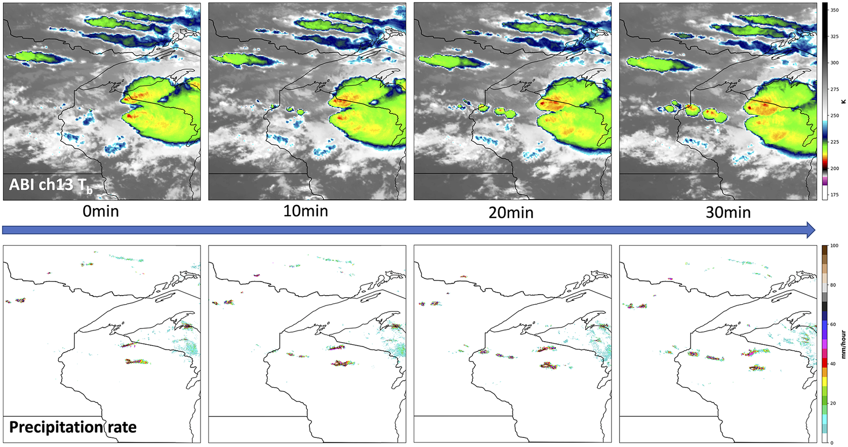
Figure 1. Sample meteorological image sequence that illustrates the importance of spatiotemporal context. Top row: Geostationary Operational Environmental Satellites (GOES)-16 Advanced Baseline Imager (ABI) Channel 13 brightness temperature at different time steps. Bottom row: corresponding Multi-Radar/Multi-Sensor System (MRMS) precipitation rate. This sequence shows the evolution of convective clouds, which is important to predict the future behavior of the developing convection.
Such temporal information is especially valuable when we want to distinguish different phenomena with similar radiometric signatures, such as bright clouds moving through the scene versus bright snow that is stationary on the ground; or when phenomena are present at different vertical levels, such as low and high clouds moving at different speeds and directions. This article provides a survey of data science approaches that can be used to recognize and utilize signals from such image sequences that span both time and space.
1.1. Sources of context
When extracting information from image sequences a key question is what kind of meteorological context is required to perform the desired task. Typical sources of context are:
-
1. Spatial context: Looking for spatial patterns in the imagery allows one to interpret values at each pixel knowing that it is part of a larger meteorological pattern, for example, part of a tropical cyclone (TC);
-
2. Temporal context: Utilizing several time steps can be useful to gain information on the temporal evolution of a phenomenon.
-
3. Multi-variable context (spectral channels or atmospheric variables): Using several satellite channels (if the imagery comes from satellites) or different atmospheric variables (if the imagery comes from models) is often helpful since different variables capture different aspects of the atmospheric (or environmental) state.
Many meteorological applications require one or more sources of context, such as spatial, temporal, and/or multi-variable context. For example, a human can identify convection more easily from sequences of satellite imagery, rather than from a single image, because convection involves the upward motion of air which results in what looks like a bubbling effect at the top of clouds and a temporal decrease in brightness—both of which are temporal changes and thus not easily identifiable in a still image. For example, in the top row of Figure 1, there is a decrease in brightness temperature in locations where the bottom row indicates increased precipitation rate. Likewise, it has been shown that neural networks can also perform this task better when given temporal sequences of imagery, as shown by Lee et al. (Reference Lee, Kummerow and Ebert-Uphoff2021). Multi-spectral context is also relevant in this application, as both visible and infrared channels provide important information. Similarly, forecasting solar radiation also benefits from providing a sequence of temporal images to a neural network architecture, as shown by Bansal et al. (Reference Bansal, Bansal and Irwin2021, Reference Bansal, Bansal and Irwin2022). These two applications are discussed in more detail in Section 2.
1.2. Visual representation, problem statement, and key challenges
Figure 2 illustrates how we represent images and image sequences throughout this article. Note in particular the directions of time (downward, yellow arrow) versus variable/channel dimension (stacked, green arrow) used for image sequences, as shown in Figure 2c,d.
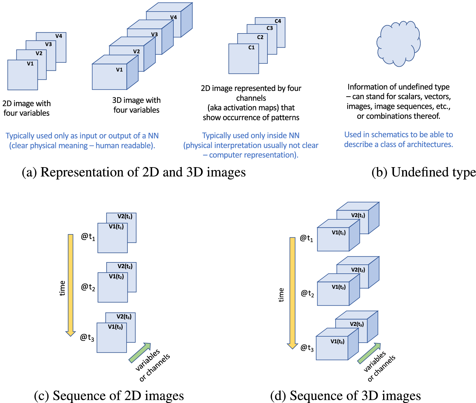
Figure 2. Visual representation of a single image (a), undefined type (b), and image sequences (c,d) used in this article. For image sequences, note that time is always represented vertically (direction of yellow arrow) and variables/channels are shown as stacks of individual 2D or 3D elements (direction of green arrow). The specific number of variables or channels shown here (four in (a); two in (c,d)) is only used for illustration, in particular, to demonstrate that the number of channels does not have to be three, as is typically assumed in computer vision applications since they tend to deal with sequences of RGB images.
Figure 3 provides a high-level overview of the problem we consider. We are given a meteorological image sequence with three types of dimensions, namely, two or more spatial dimensions ( $ {D}_i $
), a temporal dimension (T), and a multi-variable dimension (V). The task we want to achieve is to use a combination of feature engineering and machine learning to extract those spatiotemporal signals from the image sequence relevant to estimate the desired output. The desired output may be a class label (e.g., precipitation type), a scalar (e.g., estimated wind speed), an image (e.g., simulated radar, Ebert-Uphoff and Hilburn, Reference Ebert-Uphoff and Hilburn2020), or any other desired type of information.
$ {D}_i $
), a temporal dimension (T), and a multi-variable dimension (V). The task we want to achieve is to use a combination of feature engineering and machine learning to extract those spatiotemporal signals from the image sequence relevant to estimate the desired output. The desired output may be a class label (e.g., precipitation type), a scalar (e.g., estimated wind speed), an image (e.g., simulated radar, Ebert-Uphoff and Hilburn, Reference Ebert-Uphoff and Hilburn2020), or any other desired type of information.
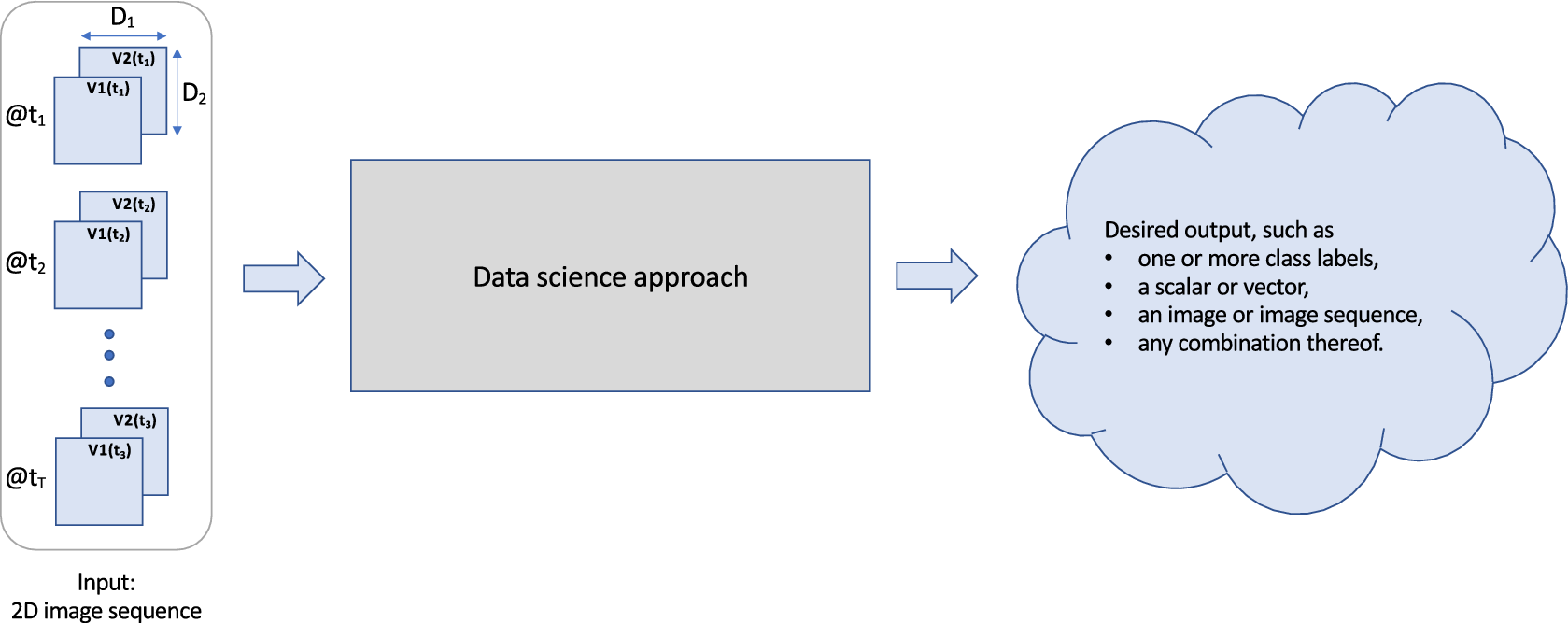
Figure 3. Problem definition for extracting spatiotemporal information from a meteorological image sequence. The dimension names of the input image sequence shown here are used throughout this document: $ {D}_i $
for spatial dimensions,
$ {D}_i $
for spatial dimensions, $ T $
for number of time steps, and
$ T $
for number of time steps, and $ V $
(here
$ V $
(here $ V=2 $
) for the number of variables.
$ V=2 $
) for the number of variables.
The key challenge to design a good method to detect all relevant spatiotemporal patterns lies in the high dimensionality of the pattern space, namely of the set of all combinations of real values extending over the entire space of spatial, temporal, and variable dimensions. For a 2D image sequence that means searching for all possible patterns in a multi-dimensional array of dimension $ \left(D1,D2,T,V\right) $
. Searching the entire space is not feasible, and thus one must find simplifications that allow us to reduce the search space while still being able to capture all physically relevant patterns of the task at hand.
$ \left(D1,D2,T,V\right) $
. Searching the entire space is not feasible, and thus one must find simplifications that allow us to reduce the search space while still being able to capture all physically relevant patterns of the task at hand.
1.3. Guiding questions
Which method is best suited to extract relevant spatiotemporal patterns depends on various properties of the considered task, including:
-
Q1: How complex are the patterns to be detected?
Simple pattern example: Area of high contrast that persists in single location over two time steps.
Complex pattern example: Cloud bubbling pattern indicating convection (see Section 2.1).
-
Q2. Is prior knowledge available regarding the patterns to be detected?
If so we can design simplified methods that only focus on a prescribed family of patterns.
-
Q3. How far does each pattern extend in space and time?
Example: Is it sufficient to consider values in close spatial and temporal proximity of each other? If so then dimensionality of the pattern search space is greatly reduced.
-
Q4. Can pattern detection be decoupled in space and time?
Example: Is it sufficient for the task to look for patterns in each image individually, then track their occurrence over time?
-
Q5. How many labeled samples are available for training?
-
Q6. How important is transparency to the end user, that is, an understanding of the strategies used by the ML model to perform its task?
-
Q7. Are any models available that have been trained on similar tasks and that could provide a starting point for this task?
These questions motivate the development and selection of the different methods discussed throughout this manuscript.
1.4. Methods discussed here
Figure 4 provides an overview of the types of tools discussed here. Section 2 provides some practical examples from our own research that demonstrate the need for utilizing spatiotemporal context contained in meteorological imagery. In Sections 3–6, we discuss four groups of approaches that each address different needs and have their own pros and cons, as outlined in Figure 4. We structure the discussion of approaches for incorporating spatial context based on how much expert knowledge they use, starting with the highest level of expert knowledge used in the feature engineering section, Section 3. Sections 4 and 5 discuss increasingly complex machine learning methods from traditional convolutional neural networks (Section 4) to advanced neural networks that use attention (Section 5). The methods discussed in Sections 3 and 4 have been widely applied and those sections make up the bulk of this manuscript. In contrast, the methods discussed in Section 5 are brand-new, and that section therefore only briefly discusses these concepts to give readers an inkling of what is yet to come. Section 6 very briefly discusses different strategies that can help reduce the need for a large number of labeled samples for training, such as self-supervised learning and transfer learning. Section 7 presents conclusions.
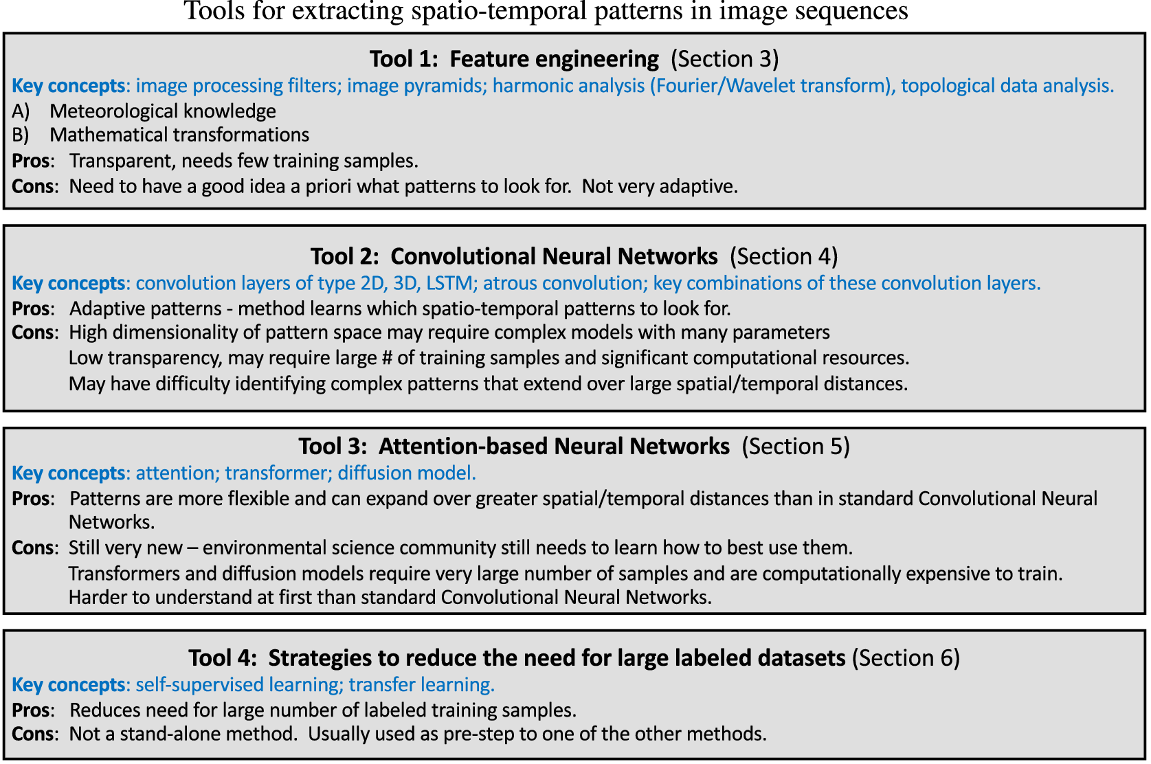
Figure 4. Overview of four types of tools discussed here, including key concepts, their pros and cons, and the sections where they are introduced. Note that this is an overview table of the paper, so it contains many concepts that have not yet been defined.
1.5. Intended audience
Sections 1–3 are written for a general audience. Sections 4–6 assume that readers are already familiar with the basic concept of convolutional neural networks (CNNs). Readers not yet familiar with that concept can gain that understanding from Lagerquist et al. (Reference Lagerquist, McGovern, Homeyer, Gagne and Smith2020) which provides an excellent introduction to the topic for environmental scientists.
2. Sample Applications Illustrating the Importance of Spatiotemporal Context
In this section, we introduce two sample applications that help illustrate the importance of utilizing the spatiotemporal context inherent in image sequences for prediction tasks in environmental science. We chose applications from our own previous work, simply because we have deeper insights into those topics. The applications are (a) detecting convection, and (b) forecasting solar radiation. Both applications use geostationary satellite image sequences as input.
2.1. Detecting convection in geostationary satellite image sequences
Convection is a rapidly developing feature, often developing within a few hours or even a few minutes. Being able to observe and predict the correct location of convection is critical in short-term forecasts, especially to warn the public about the hazards such as strong winds, flooding, tornadoes, or hail events. Radar reflectivity from ground-based radar is a good indicator of precipitation intensity, which is closely related to convection intensity, and thus radar reflectivity is the primary observation currently used for convection detection as well as short-term precipitation forecast. Despite radar reflectivity providing high accuracy and high-temporal resolution data suitable for short-term forecasts, ground-based radar has its own limitation of less coverage over mountainous regions and the ocean. Outside of ground-based radar coverage, a geostationary satellite is the only observation continuously available for convection detection.
It is challenging to use geostationary satellites as their visible or infrared data only provide cloud-top information, but their high-temporal resolution allows us to better observe the development of convective clouds. As shown in Figure 1, a decrease in brightness temperature and a divergence observed at cloud top are two of the features of convective clouds observed from geostationary satellite images, but cannot be observed if looking at a static image. With the help of machine learning techniques, it has become easier to extract spatial and temporal features of convective clouds. Features of convective clouds that can be observed by visible and infrared sensors on geostationary satellites are high reflectance, low brightness temperature, bubbling cloud top, and decreasing brightness temperature. We can somewhat detect convection by looking at high reflectance and low brightness temperature in a static image, but the bubbling cloud top signal that is characteristic of convection stands out much more in temporal image sequences. Similarly, decrease in brightness temperature is a feature that can only be observed by the temporal image sequences. Lee et al. (Reference Lee, Kummerow and Ebert-Uphoff2021) explore the use of temporal image sequences from GOES-16 to detect convection, and the results are validated against one of the ground-based radar products called multi-radar/multi-sensor system (MRMS). They show that using image sequences provided slightly better results than using a static image. This application is used to illustrate the concepts in Section 4.4.
2.2. Nowcasting solar radiation
Solar power is the cheapest form of electricity in history but its contribution to the electric grid remains low. This is mainly because of solar energy’s variability that changes with the amount of downwelling radiation that reaches the Earth’s surface. Effectively predicting the amount of irradiance is akin to forecasting the amount of solar energy produced by solar panels because of the strong correlation between the two (Raza et al., Reference Raza, Nadarajah and Ekanayake2016). Many techniques have been proposed in the past to address this problem including NWP algorithms (Mathiesen and Kleissl, Reference Mathiesen and Kleissl2011; Chen et al., Reference Chen, He, Chen, Hu and He2017; Tiwari et al., Reference Tiwari, Sabzehgar and Rasouli2018; Gamarro et al., Reference Gamarro, Gonzalez and Ortiz2019), that mostly leverage physics-based modeling. These are often used for solar irradiance forecasting, and are most appropriate for forecast horizons on the scale of hours to days, but not for nowcasting on the scale of minutes to an hour (Hao and Tian, Reference Hao and Tian2019; Wang et al., Reference Wang, Lei, Zhang, Zhou and Peng2019).
The other way of tackling this problem is with machine learning approaches that have the potential to implicitly model local changes from observational data (Wang et al., Reference Wang, Lei, Zhang, Zhou and Peng2019; Rolnick et al., Reference Rolnick, Donti, Kaack, Kochanski, Lacoste, Sankaran, Ross, Milojevic-Dupont, Jaques, Waldman-Brown, Luccioni, Maharaj, Sherwin, Mukkavilli, Kording, Gomes, Ng, Hassabis, Platt, Creutzig, Chayes and Bengio2022) like analyzing images from ground-based sky cameras (Zhang et al., Reference Zhang, Verschae, Nobuhara and Lalonde2018; Siddiqui et al., Reference Siddiqui, Bharadwaj and Kalyanaraman2019; Zhao et al., Reference Zhao, Wei, Wang, Zhu and Zhang2019; Paletta and Lasenby, Reference Paletta and Lasenby2020) and estimating cloud motion vectors (Lorenz et al., Reference Lorenz, Hammer and Heinemann2004; Lorenz and Heinemann, Reference Lorenz and Heinemann2012; Cros et al., Reference Cros, Liandrat, Sébastien and Schmutz2014) from satellite images. However, installing sky cameras requires additional infrastructure making the approach less scalable. Instead, ML approaches that model solar irradiance tend to perform better (Lago et al., Reference Lago, De Brabandere, De Ridder and De Schutter2018; Bansal and Irwin, Reference Bansal and Irwin2020) in comparison to the other approaches. Bansal et al. (Reference Bansal, Bansal and Irwin2022) propose an approach for solar nowcasting by forecasting solar irradiance values from multispectral visible bands from GOES satellite data using the approach shown in Figure 5. This approach uses a neural network model that is a combination of a spatial extraction followed by temporal extraction ML model (center panel) that forecasts values of the satellite channels at a future time, $ t+1 $
, which are in turn used to predict solar output at a future time (right panel). This application thus uses spatial, temporal, and spectral information in its prediction of a future value of the satellite’s visible channels. This application is used to illustrate the concepts in Section 4.3.
$ t+1 $
, which are in turn used to predict solar output at a future time (right panel). This application thus uses spatial, temporal, and spectral information in its prediction of a future value of the satellite’s visible channels. This application is used to illustrate the concepts in Section 4.3.
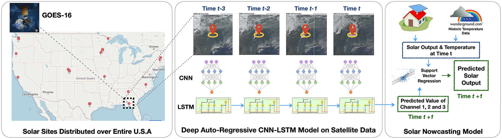
Figure 5. Solar nowcasting application from Bansal et al. (Reference Bansal, Bansal and Irwin2022). Multispectral satellite data are collected from 25 U.S. sites (see left panel), then sequences of observations at each site, specifically the first three spectral channels (visualized in the middle), are used as input to a neural network model (see center panel), which is trained to predict the three-channel values at the center (red pin) for the next time step ( $ t+1 $
). A simple machine learning algorithm (see right panel), namely an auto-regressive support vector regression model, takes the predicted scalar channel values, previous solar output, and previous temperature, to predict the solar output at (
$ t+1 $
). A simple machine learning algorithm (see right panel), namely an auto-regressive support vector regression model, takes the predicted scalar channel values, previous solar output, and previous temperature, to predict the solar output at ( $ t+1 $
). See Bansal et al. (Reference Bansal, Bansal and Irwin2022) and Section 4.3 for more explanation. This figure is adapted and used with due permission from Bansal et al. (Reference Bansal, Bansal and Irwin2022). ©Author(s) of Bansal et al. (Reference Bansal, Bansal and Irwin2022). Contact the copyright holder for further reuse.
$ t+1 $
). See Bansal et al. (Reference Bansal, Bansal and Irwin2022) and Section 4.3 for more explanation. This figure is adapted and used with due permission from Bansal et al. (Reference Bansal, Bansal and Irwin2022). ©Author(s) of Bansal et al. (Reference Bansal, Bansal and Irwin2022). Contact the copyright holder for further reuse.
3. Feature Engineering: Constructing Strong Signals for ML Methods to Use
The meteorological community often uses the term (statistical) predictors to refer to quantities that are deemed important for the prediction of quantities to be estimated (predictands). In the machine learning literature, the predictors are known as features. We will use the two terms predictor and feature interchangeably throughout this article. Feature selection refers to the process of selecting key predictors from a large set of possible predictors, for example, choosing which satellite channels contain the most information. Feature engineering goes further by creating new features from the considered set of predictors. For example, teleconnection indices, such as the North Atlantic Oscillation (NAO), West Pacific Oscillation (WPO), East Pacific Oscillation (EPO) (Barnston and Livezey, Reference Barnston and Livezey1987), Pacific/North American Pattern (PNA) (Wallace and Gutzler, Reference Wallace and Gutzler1981), and arctic oscillation (AO) (Thompson and Wallace, Reference Thompson and Wallace1998) are scalar features extracted from atmospheric fields, developed over decades to capture key information about the atmospheric state in a minimal representation. A simpler example is the split window difference of satellite channels, that is, the difference between two different channels, which experts know contains specific information relevant to a problem, such as dust detection (Miller et al., Reference Miller, Grasso, Bian, Kreidenweis, Dostalek, Solbrig, Bukowski, van den Heever, Wang, Xu, Wang, Walker, Wu, Zupanski, Chiu and Reid2019) or estimating low-level moisture (Dostalek et al., Reference Dostalek, Grasso, Noh, Wu, Zeitler, Weinman, Cohen and Lindsey2021). More generally, feature engineering seeks to extract key information and make it easily accessible for subsequent models, such as statistical or machine learning models. Engineered features may achieve dimension reduction—the teleconnection indices are an extreme example of this—or it may retain the original dimension and instead amplify a key signal in the data that makes subsequent analysis more robust and successful.
3.1. Meteorologically motivated image features (most transparent)
Meteorologists have developed a rich set of statistical predictors for any meteorological application one can think of. Over decades such predictors were carefully designed using expert intuition, and refined through testing to yield the best predictions possible when feeding them as inputs into statistical or, more recently, machine learning methods. This includes predictors obtained from imagery.
For example, in the area of TCs, the statistical hurricane intensity prediction scheme (SHIPS; DeMaria and Kaplan, Reference DeMaria and Kaplan1994) defines a set of predictors that are deemed useful to predict properties of TCs, such as future TC intensity and location. Newer versions of the SHIPS database (RAMMB, Reference Rammb2022) include scalar predictors obtained from satellite imagery, such as the minimum, maximum, average, or standard deviation of the brightness temperature within certain radii from the storm center; fraction of area with brightness temperatures colder than particular thresholds; or principal component analysis (Knaff et al., Reference Knaff, Slocum, Musgrave, Sampson and Strahl2016).
The Warning Decision Support System—Integrated Information, aka WDSS-II, developed by the National Severe Storm Laboratory (NSSL) is a real-time system used by the National Weather Service to analyze weather data (Lakshmanan et al., Reference Lakshmanan, Smith, Stumpf and Hondl2007). This system uses morphological image processing techniques to extract storm cells from images (Lakshmanan et al., Reference Lakshmanan, Hondl and Rabin2009), track those cells in time (Lakshmanan and Smith, Reference Lakshmanan and Smith2010), and compute statistics and time trends of storm attributes for the cells (Lakshmanan and Smith, Reference Lakshmanan and Smith2009).
The advantages of using meteorologically motivated features are that they may provide dimensionality reduction, enhance the strength of key signals, and provide models that are physically interpretable. We believe that feature engineering methods are sometimes under-utilized when advanced machine learning methods are employed. Feature engineering should be kept in mind as a powerful means to infuse physical knowledge into machine learning, and thus to simplify ML models and improve their transparency and robustness.
3.2. Mathematically motivated image features (moderately transparent)
This section briefly discusses three mathematical frameworks that can help to extract spatial features of images in the context of neural networks. We feel that all of these methods are currently under-utilized in environmental science and should receive more attention. This is by no means a complete list, we are certain that there are other important mathematical tools we have not thought of. The three frameworks discussed below only cover those our group has tried for environmental applications.
3.2.1. Classic image processing tools and image pyramids
Traditional satellite retrieval techniques tend to either treat individual satellite pixels as being independent or they make use of simple spatial information, such as the standard deviation in a neighborhood (Grecu and Anagnostou, Reference Grecu and Anagnostou2001). The information content in spatial patterns is an important factor in the ability of convolutional NNs to outperform traditional methods (Guilloteau and Foufoula-Georgiou, Reference Guilloteau and Foufoula-Georgiou2020). However, the myriad of filters learned by Convolutional NNs may not always be necessary. Instead, concepts from classic image processing can be used to extract spatial information (Hilburn, Reference Hilburn2023). For example, key spatial information can be extracted using (a) predefined filters to extract specific image properties, for example, the local mean or gradient of an image; and (b) image pyramids that represent images at different resolutions (Burt and Adelson, Reference Burt and Adelson1983; Adelson et al., Reference Adelson, Anderson, Bergen, Burt and Ogden1984), which provides a representation of multi-scale information in the images. We believe that these classic tools are under-utilized ever since CNNs became popular in our research community. Many ML algorithms could be made much simpler, more robust, and more interpretable, through more extensive use of feature generation using these classic methods, specifically by using image pyramids combined with classic filters to generate stronger features that can be used with simpler machine learning methods (Hilburn, Reference Hilburn2023), for example, support vector machines or random forest instead of convolutional NNs.
3.2.2. Harmonic analysis (Fourier and Wavelet transforms)
Another way to extract and utilize spatial information by mathematical means is to apply harmonic analysisFootnote 1 to obtain spectral properties of images, for example, by transforming images using the spatial version of the Fourier or wavelet transforms. The properties in spectral space, for example, the presence of high-magnitude signals of certain (spatial) frequencies, can be efficient features for the occurrence of certain patterns. More complex examples of using harmonic analysis in combination with machine learning for meteorological imagery include the use of harmonic analysis in neural network to focus on specific spatial scales (Lagerquist and Ebert-Uphoff, Reference Lagerquist and Ebert-Uphoff2022) and the use of Wavelet neural networks (Stock and Anderson, Reference Stock and Anderson2022).
3.2.3. Topological data analysis
Topological data analysis (TDA) provides several tools to extract topological properties from meteorological imagery. For example, the topological concept of persistent homology focuses on the number of connected regions, and the number of holes therein, for a varying intensity threshold in the image, which in turn allows to distinguish different types of patterns, for example, to classify the mesoscale organization of clouds (Ver Hoef et al., Reference Ver Hoef, Adams, King and Ebert-Uphoff2023). Persistent homology and other topological properties are emerging in several environmental science and related applications, including in the context of identifying atmospheric rivers (Muszynski et al., Reference Muszynski, Kashinath, Kurlin and Wehner2019), Rossby waves (Merritt, Reference Merritt2021), local climate zones (Sena et al., Reference Sena, da Paixão and de Almeida França2021), activity status of wildfires (Kim and Vogel, Reference Kim and Vogel2019), and quantifying the diurnal cycle of TCs (Tymochko et al., Reference Tymochko, Munch, Dunion, Corbosiero and Torn2020). Generally, TDA is not used as standalone technique, but as a preprocessing step to extract important features, often to be used along with other physically interpretable features, followed by a simple machine learning algorithm, for example, support vector machines.
3.3. Image features learned by neural networks (least transparent)
While simple machine learning algorithms, such as linear regression and decision trees, are fairly transparent, neural network models, such as the models discussed in Section 4, tend to be opaque. In fact, a basic idea behind neural networks is that they gradually construct their own features in the so-called “hidden” layers of the network, and those features are very hard to decipher. For example, convolutional neural networks, which are discussed in detail in the next section, learn features in the form of convolution filters, rather than using predefined convolution filters from classic image processing (Section 3.2.1).
One can try to gain an understanding of a CNN by analyzing the individual filters it has learned. However, that is a challenging task because CNNs use many layers of filters stacked on top of each other that in combination extract patterns. Therefore, investigating a single learned filter in isolation is usually not sufficient to reveal its purpose in the entire network. This is why many Explainable AI methods, such as attribution maps (McGovern et al., Reference McGovern, Lagerquist, Gagne, Jergensen, Elmore, Homeyer and Smith2019; Ebert-Uphoff and Hilburn, Reference Ebert-Uphoff and Hilburn2020), seek to develop an understanding of the NN’s strategies by focusing on the functionality of the entire neural network, rather than of individual filters (Olah et al., Reference Olah, Mordvintsev and Schubert2017). Explainable AI is helpful and sometimes allows one to identify features that a NN is paying attention to (Ebert-Uphoff and Hilburn (Reference Ebert-Uphoff and Hilburn2020)), but it is not a magic bullet, and certainly not a replacement for designing ML methods that are a priori interpretable (Rudin, Reference Rudin2019). Thus, we believe that for the great majority of environmental science applications (there are exceptions!) one should seek to maximize the use of meteorologically and mathematically motivated image features first, then apply a simpler ML method that builds on these features. This philosophy might run counter to the traditional view in the AI community to leave all learning to the ML algorithm. However, this philosophy is often called for by the special needs of typical environmental science applications, such as (a) significant knowledge of key patterns, (b) small number of available training samples, and (c) use as a decision support tool for high stake decisions (e.g., severe weather warnings or climate policy decisions) that require a higher standard of transparency.
4. Convolutional Neural Networks to Analyze Image Sequences
Once feature engineering methods have been applied as much as possible to create stronger signals, machine learning methods can be used on top of those features. In this section, we focus on convolutional neural networks (CNNs), which have become a very popular tool for image tasks in meteorology. CNNs build on the traditional concept of image filters and image pyramids discussed in Section 3.2.1, but instead of using predefined filters, CNNs learn their own filters, which makes them much more flexible and allows them to identify a greater variety of spatial patterns. Given a billion training samples with accurate labels, CNNs can learn extremely complex patterns. However, in meteorological applications, there are often relatively few labeled samples available. Thus, when we use CNNs to extract spatiotemporal patterns from meteorological image sequences, we need to weigh the complexity of the CNN, in particular the number of parameters to be learned, against the number of available training samples. This motivates the search for simple architectures that work for a given task, rather than insisting that any type of spatiotemporal pattern can be found. As we will see, different CNN architectures make different assumptions about patterns to be recognized and achieve different trade-offs regarding pattern flexibility versus model complexity.
In this section, we focus on relatively simple CNNs that use as building blocks layers of type conv2D, conv3D, LSTM, and convLSTM. The names of these layers are from the TensorFlow/Keras (Abadi et al., Reference Abadi, Agarwal, Barham, Brevdo, Chen, Citro, Corrado, Davis, Dean, Devin, Ghemawat, Goodfellow, Harp, Irving, Isard, Jia, Jozefowicz, Kaiser, Kudlur, Levenberg, Mane, Monga, Moore, Murray, Olah, Schuster, Shlens, Steiner, Sutskever, Talwar, Tucker, Vanhoucke, Vasudevan, Viegas, Vinyals, Warden, Wattenberg, Wicke, Yu and Zheng2016) programming environment. Equivalent layers exist in PyTorch and other standard neural network development frameworks. We assume that readers are familiar with the basic concepts of CNNs, such as 2D convolution layers, pooling layers, and so forth. See LeCun et al. (Reference LeCun, Boser, Denker, Henderson, Howard, Hubbard and Jackel1989) and LeCun and Bengio (Reference LeCun and Bengio1998) for an introduction to those topics.
This section is organized as follows. We first introduce spatial convolution layers and several ways for how to use them for image sequences (Section 4.1). Section 4.2 discusses recurrent neural networks (RNNs), both LSTM and convLSTM. The remaining sections illustrate how these building blocks can be combined into architectures (Section 4.3), and compare the practical use of conv2D, conv3D, and convLSTM layers for the convection application (Section 4.4).
4.1. Spatial convolution layers and ways to use them for image sequences
In this section, we discuss spatial convolution layers, conv2D and conv3D. We first illustrate their originally intended use, which was for finding patterns in individual images, then discuss how they can be used nevertheless to extract spatiotemporal patterns in image sequences.
4.1.1. Originally intended use of conv2D and conv3D
Figure 6 illustrates the originally intended use of spatial convolution layers, conv2D and conv3D. As shown in the figure, both were originally designed to extract patterns from individual images.
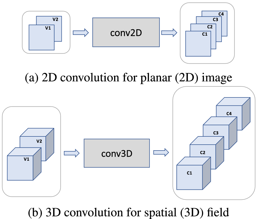
Figure 6. Spatial convolution layers, conv2D and conv3D, were originally designed to extract patterns from an individual image, not from an image sequence. The input is a single image (2D image in [a], 3D image in [b]), and the output is a set of channels, aka activation maps. Each channel corresponds to one spatial pattern, which is learned during training and represented by the filter weights, and tracks the location and strength of occurrence of that pattern in the input image. The number of input variables (two) and output channels (four) shown here is arbitrary.
4.1.2. Time-to-variable
While conv2D and conv3D were originally designed to extract patterns from individual images, they have also been used for image sequences in a different fashion. The first type of use is by treating time as a variable, as illustrated in Figure 7. Here an image sequence is first converted to a single image by treating the images at different time steps as if they were additional variables. Resulting properties are:
-
1. The meaning of the order and adjacency of time steps is lost to the network since they are treated as additional variables, and the order of variables is ignored in neural networks.
-
2. At the output of conv2D, the time steps are no longer represented separately, that is, the time dimension has collapsed. Thus all patterns of interest that span different time steps must be identified by this layer. No other temporal patterns can be identified by a sequential model after conv2D has been applied in this way. One should thus carefully consider how early in a network conv2D can be used in this fashion.
-
3. This approach results in significant dimensionality reduction, so a model with fewer parameters, thus suitable for small sample size.
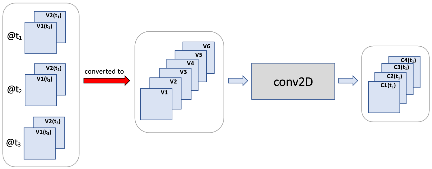
Figure 7. Time-to-variable: Use of conv2D for a 2D image sequence by first converting the image sequence to a single image with additional variables. The time dimension is thus converted to an increase in variable dimension, that is, time is treated as variables. (The same logic can be applied to 3D image sequences by replacing all 2D by 3D images in the schematic, and applying conv3D.)
4.1.3. Time-to-space
In Figure 8, the time dimension is treated as third spatial dimension. Resulting properties are:
-
1. The third spatial dimension is preserved by conv3D, thus time steps are still represented separately in the output, and their order and adjacency are preserved.
-
2. Spatial convolutions have well-known boundary effects. Namely, the information content at and near the image boundaries tends to decrease with each application of a convolution layer. In large images, this effect can often be ignored. However, given that there are often only fewer than 10-time steps considered, this effect could become significant. Thus, if conv3D is applied repeatedly to a time sequence while time is represented as third spatial dimension, it is possible that the patterns involving the first and last images of an image sequence have less of an impact. Unfortunately, the last image is typically the most recent image which tends to be very important, especially for prediction tasks.
-
3. Model complexity for the time-to-space approach tends to be significantly higher than for the time-to-variable approach, since the time dimension is preserved and carried through to later layers.
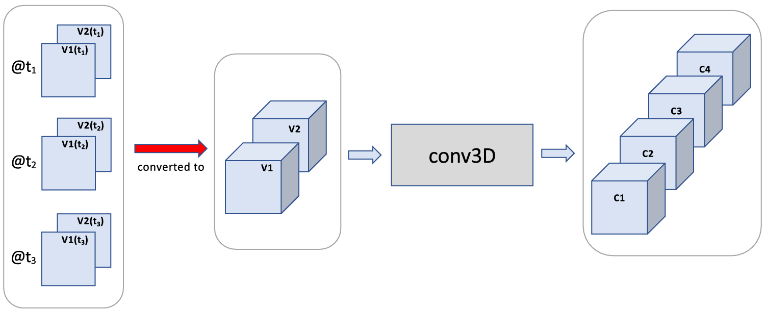
Figure 8. Time-to-space: Use of conv3D for a 2D image sequence by first converting the time dimension to a third spatial dimension.
4.1.4. Dilated or atrous convolution layer to increase receptive field size
One important concept to consider when designing a CNN model is its receptive field (Araujo et al., Reference Araujo, Norris and Sim2019), that is, the size of the region in the input image that affects the value of a NN output. In the context of detecting spatiotemporal patterns the receptive field is important because it provides the maximal pattern size in the input image that the NN can recognize, see Ebert-Uphoff and Hilburn (Reference Ebert-Uphoff and Hilburn2020) for a longer discussion. Well-known ways to increase the size of receptive fields and extract large-scale features are to (a) add pooling layers, that is, reduce resolution before the next convolution layer, or (b) use a stride size bigger than one, that is, moving the convolution filter in larger increments. Another option that is very effective but much less known is the concept of dilated (Yu and Koltun, Reference Yu and Koltun2016) or atrous (Chen et al., Reference Chen, Papandreou, Kokkinos, Murphy and Yuille2018) convolution. An atrous convolution layer stretches the convolution filter to cover a larger area without increasing the number of parameters or reducing resolution. For example, a 3 × 3 filter can be stretched to cover a 5 × 5 area of pixels by ignoring every second pixel (imagine a checkerboard pattern as a convolution filter where only the white squares are utilized). Atrous convolutions expand the receptive field exponentially without loss of resolution or coverage, see Yu and Koltun (Reference Yu and Koltun2016). Atrous convolutions can be very helpful to extract large-scale features, while maintaining resolution of the output image.
Environmental science examples: Many applications use atrous convolution layers for classification problems. Zhan et al. (Reference Zhan, Wang, Shi, Cheng, Yao and Sun2017) use atrous convolution layers for classifying snow and cloud, Kanu et al. (Reference Kanu, Khoja, Lal, Raghavendra and CS2020) for cloud classification, Sun et al. (Reference Sun, Zhang, Dong, Lguensat, Yang and Lu2021) for ocean eddy detection, Li and Chen (Reference Li and Chen2019) for land cover classification, and FogNet (Kamangir et al., Reference Kamangir, Collins, Tissot, King, Dinh, Durham and Rizzo2021) for visibility classification due to coastal fog.
4.2. RNNs: LSTM and convLSTM
So far we focused on utilizing CNN layer types originally intended to extract spatial patterns, such as conv2D and conv3D. In contrast, RNNs are a special type of neural network developed specifically to extract and utilize patterns in scalar time series, for example, to be able to predict a value at the next time step given values at prior time steps. RNNs were developed to resolve temporal relationships within input data by keeping the past memory and carrying it to the next state (Rumelhart et al., Reference Rumelhart, Hinton and Williams1985; Jordan, Reference Jordan1986). This is achieved by maintaining memory about the past state in the form of one or more hidden (aka latent or internal) variables that are carried forward and used as input to the next time step. (At the start the hidden variables get default values as no meaningful information is available.) However, standard RNNs suffer from having a short memory, that is, values from the past are assumed to quickly lose relevance as time progresses. They also suffer from the vanishing gradient problem, which is a common problem during NN training where gradients become so small that they no longer propagate useful information backward to adjust the parameters of the NN model. In order to overcome the vanishing gradient problem and to ensure that memory of early time steps is carried through to much later time steps, the long–short-term memory (LSTM) architecture was developed (Hochreiter and Schmidhuber, Reference Hochreiter and Schmidhuber1997). LSTM layers are designed to learn which information to keep or forget (Gers et al., Reference Gers, Schmidhuber and Cummins2000). LSTMs have become the dominant type of RNNs used in environmental science applications.
Since LSTM layers are designed to extract temporal patterns only from scalar time series, how can they be used for image time series? There are two primary options:
-
1. LSTM layers can be used after spatial patterns have been reduced to scalar features (e.g., see Figure 5). This approach is discussed in Section 4.3.
-
2. The LSTM layer concept has been expanded to images, leading to convLSTM layers. Namely, the convLSTM operator (Figure 9) is a convolution version of the LSTM operator developed for video or image sequences to extract spatiotemporal features. This approach is discussed below.
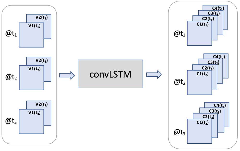
Figure 9. The convLSTM layer was designed specifically to extract spatiotemporal patterns from an image sequence, for example, for predicting the next image in a sequence given prior images. The output of the convLSTM layer shown here has as many time steps as the input. This form is usually used in earlier CNN layers. Another form, which is usually used toward the end of the CNN, outputs a single image, for example, the predicted image at the next time step. A hyperparameter, chosen by the CNN developer, determines which form is used for each convLSTM layer.
The remainder of this subsection discusses the second option above, convLSTM layers (Shi et al., Reference Shi, Chen, Wang, Yeung, Wong and Woo2015). First, for the benefit of those readers familiar with LSTM, but not convLSTM, we briefly describe the difference. LSTM is generalized to convLSTM as follows: In LSTM layers all gates are vectors, that is, 2D tensors including channel dimension. In convLSTM layers all gates are images, that is, 3D tensors including channel dimension. Consequently, the matrix multiplications between weight matrices and gates in LSTM are replaced by convolution operations in ConvLSTM. ConvLSTM developed by Shi et al. (Reference Shi, Chen, Wang, Yeung, Wong and Woo2015) is already implemented in many NN libraries, such as TensorFlow. Lastly, note that ConvLSTM is based on the LSTM variant with so-called peephole connections developed by Gers and Schmidhuber (Reference Gers and Schmidhuber2000), which adds previous cell state information in the gates.
Resulting properties of using a convLSTM layer are:
-
1. The time dimension is preserved by the convLSTM layer type shown in Figure 9, that is, time steps are still represented separately in the output, and their order and adjacency are preserved.
-
2. The number of parameters of convLSTM tends to be higher, comparable to the time-to-space approach in Section 4.1.3.
-
3. The logic of convLSTM layers is much more complex than of conv2D and conv3D, making them harder to apply. In our personal experience with this and other applications, we found it much trickier to train a convLSTM layer successfully than any of the other layers. This is likely due to two factors: (a) convLSTM layers have a more complex logic so require more expertise to tune. (b) ConvLSTM layers have more parameters and thus require a large sample size. Our applications might have too few training examples. However, other research groups have found convLSTM to work well for their applications (see examples below).
Environmental science examples: ConvLSTM is used for example for precipitation forecasting (Shi et al., Reference Shi, Chen, Wang, Yeung, Wong and Woo2015; Kim et al., Reference Kim, Hong, Joh and Song2017; Wang and Hong, Reference Wang and Hong2018; Akbari Asanjan, Reference Akbari Asanjan2019; Ehsani et al., Reference Ehsani, Zarei, Gupta, Barnard, Lyons and Behrangi2022) and hurricane forecasting (Kim et al., Reference Kim, Kim, Lee, Yoon, Kahou, Kashinath and Prabhat2019; Udumulla, Reference Udumulla2020).
4.3. An organizing principle: First space, then time
In our search for trade-offs between flexibility in patterns to be recognized versus model complexity, one approach stands out as very common in literature, namely what we call the first-space-then-time approach. This approach is based on the observation that images typically contain significant redundant or irrelevant information, that is, not all values of all pixels are important. This tends to be true for meteorological imagery as well. Thus, one may try to reduce dimensionality in the spatial dimension first, as indicated by the generic architecture in Figure 10.
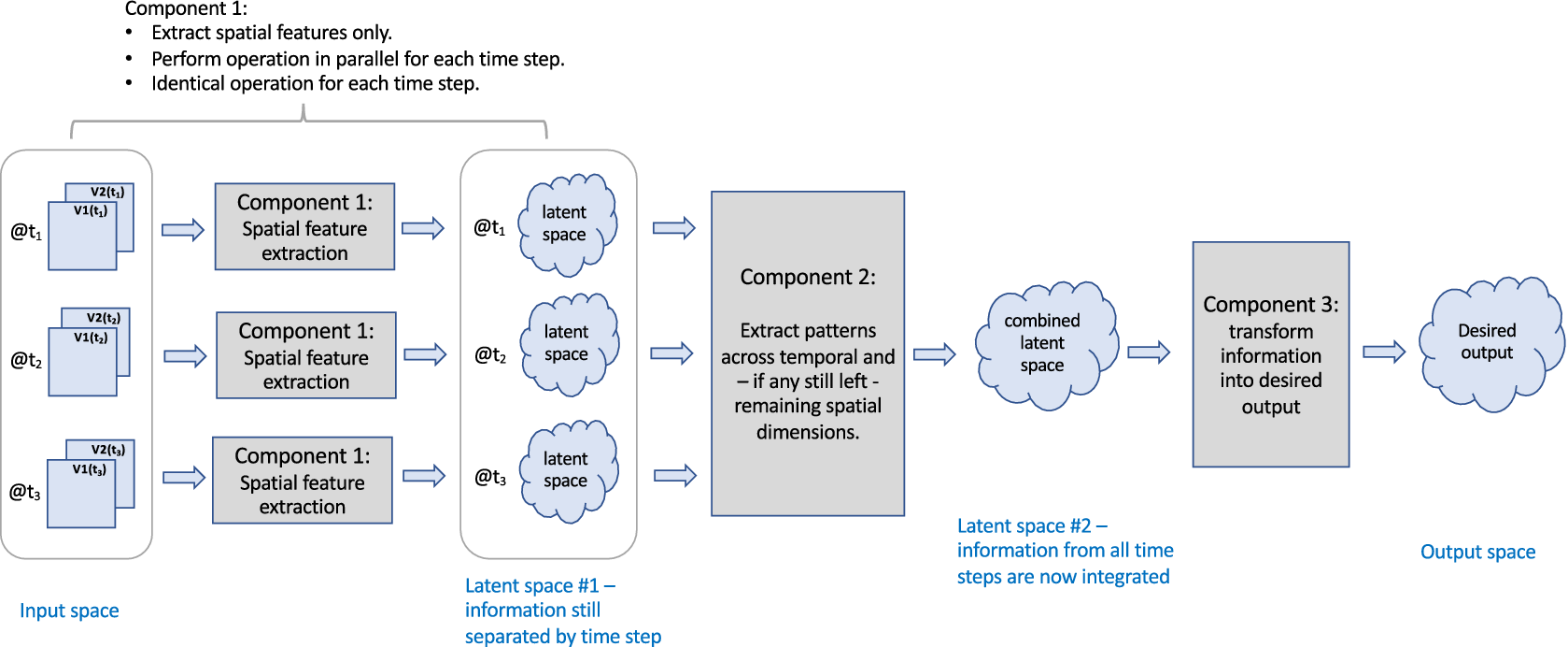
Figure 10. Generic structure of the first-space-then-time approach. Components can consist of NN layers or other ML methods.
Figure 10 uses the term latent layer. For readers not familiar with that concept, here is a brief introduction. When feeding a sample into the input layer of NN to generate a corresponding output, the information about the sample passes from the input layer through other layers to the output layer. Each layer represents information in its own way, so the input sample is represented differently in each layer. This internal representation is called the latent representation of the sample, and the corresponding space is called the latent space of that layer.
The architecture consists of three components: the first component extracts spatial information from the input sequence, resulting in Latent space 1. This first component is often a CNN, applied separately to the imagery of each time step.Footnote 2 The second component extracts the remaining spatiotemporal patterns from Latent space 1, and the third component transforms the resulting spatiotemporal information from Latent space 2 into the desired output. The key question to ask for the design of this type of architecture is as follows: How much spatial information can we meaningfully extract from each image separately in Component 1, before taking temporal information into account in Component 2?
The answer to this question determines how far the dimensionality of the input images can be reduced in the first step, that is, how small we can make the representation of each image in Latent space 1 in Figure 10, before considering time. Component 2, that is, extracting the combined spatiotemporal pattern, is often implemented using (a) conv2D with the time-to-variable approach, (b) conv3d with the time-to-space approach, or (c) convLSTM. In some applications, such as the solar forecasting application discussed below, the spatial pattern can even be expressed in scalars at the output of Component 1, so that scalar LSTM layers are sufficient for Component 2. Yet another approach is the method of temporal convolutional networks (TCNs) proposed by Lea et al. (Reference Lea, Vidal, Reiter and Hager2016) for the task of temporal action segmentation in videos, that is, assigning an action label to each frame of an image sequence. TCNs consist of a CNN for Component 1 and a combination of 1D convolution, pooling, and other layers for Component 2, see Lea et al. (Reference Lea, Vidal, Reiter and Hager2016) for details.
Environmental science example: The solar forecasting application discussed in Section 2 and introduced in Figure 5 uses the first-space-then-time principle. Figure 11 shows that architecture in terms of the components of Figure 10 from the work by Bansal et al. (Reference Bansal, Bansal and Irwin2021, Reference Bansal, Bansal and Irwin2022). The architecture first uses a CNN model to extract the spatial or channel information stored in an image tile and then applies a one-layer LSTM on top of it to extract the temporal information from the time-series visible channels from the GOES-16 satellite. Here, the idea is to simply predict the satellite’s channel value as a point value in the future. They train CNN spatial extraction and LSTM temporal models to capture the dynamics of the multispectral satellite data. After each image goes for visual feature extraction through the CNN, the per-instant spatial features extracted from CNN over time are passed through the LSTM module. LSTMs make use of both a cell state, that is, an internal memory and a hidden state and update the cell state by combining it with the current input and previous hidden state. By recursively reapplying the same function at every time step, the LSTM models the evolution of the input features over time.
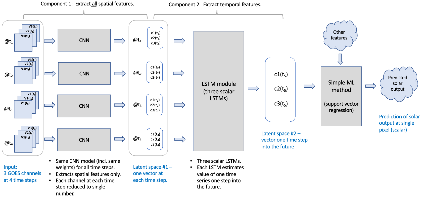
Figure 11. The architecture developed by Bansal et al. (Reference Bansal, Bansal and Irwin2022) for solar forecasting uses the first-space-then-time approach. This is the same architecture as shown in Figure 5 but shown in a way that emphasizes its first-space-then-time components.
4.4. Comparing the use of conv2D, conv3D, and convLSTM for the convection application
In this section, we compare the use of different convolution layers for the example of detecting convection discussed in Section 2.1 and by Lee et al. (Reference Lee, Kummerow and Ebert-Uphoff2021). Figure 12 describes the overall set-up used by Lee et al. (Reference Lee, Kummerow and Ebert-Uphoff2021), which is an encoder–decoder architecture. Encoder–decoder architectures are common in image-to-image translation problems, where both the input and the output are an image or image sequence. In this application, the input is an image sequence and the output is an image, namely a map indicating the probability of convection for every pixel. Both the encoder and decoder consist of several blocks of convolution and pooling layers. The purpose of the encoder is to extract spatiotemporal information, and the purpose of the decoder is to translate that spatiotemporal information into the output image (Ebert-Uphoff and Hilburn, Reference Ebert-Uphoff and Hilburn2020).
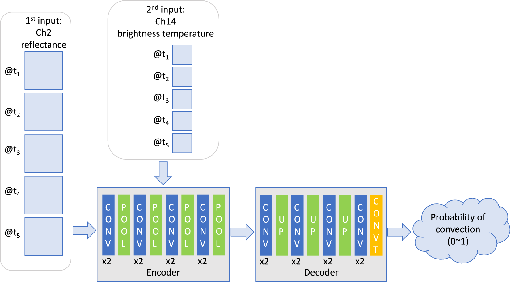
Figure 12. NN architecture used here to compare the use of different convolution layers for a real-world example, namely an encoder–decoder model to detect convection (Section 2.1; Lee et al., Reference Lee, Kummerow and Ebert-Uphoff2021). CONV, POOL, UP, and CONVT refer to convolution layer, maxpooling layer, upsampling layer, and transposed convolution layer, respectively. A sequence of high-resolution input data (Channel 2 reflectance) is ingested in the first layers, and a sequence of lower-resolution input data (Channel 14 brightness temperature) is ingested after two maxpooling layers in the encoder part. We implement the convolution layers in the encoder and decoder blocks using three different convolution layers, conv2D, conv3D, and convLSTM, and compare the results.
This study greatly extends the study by Lee et al. (Reference Lee, Kummerow and Ebert-Uphoff2021). Namely, Lee et al. (Reference Lee, Kummerow and Ebert-Uphoff2021) only looked at using conv2D layers in the encoder and decoder blocks, while here we also explore the use of conv3D and convLSTM blocks for that purpose. The encoder–decoder model architecture that is used to detect convection from GOES-16 by Lee et al. (Reference Lee, Kummerow and Ebert-Uphoff2021) is presented in Figure 12. The model uses as inputs two types of temporal image sequences from GOES-16, specifically of channel 2 reflectance and channel 14 brightness temperature. As output, it uses a convective/nonconvective classification derived from the “PrecipFlag” of the MRMS dataset (see Section 2.1). As shown in Figure 12, channel 2 reflectance data are inserted in the beginning. Channel 14 data have four times coarser spatial resolution than channel 2 reflectance data and are therefore inserted after two maxpooling layers in the encoder. In this model setup, five channel 2 temporal image sequences are treated as five different variables in the input layer, and five channel 14 images are added as five different channels in the hidden layer. One advantage of this approach is that the training is fast, and the results are shown to be comparable to the radar product.
For this extended study, we designed an experiment with nine different configurations to explore the impact of using different convolution blocks and different time intervals between the input images. Namely, we use three different convolution layers (conv2D, conv3D, and convLSTM2D) and three different datasets. The only difference between the three datasets was how many images and at what temporal distance are used in the input. Data set 1 uses three images with 4-min intervals ( $ t-8,t-4,t $
). Data set 2 uses five images with 2-min intervals (
$ t-8,t-4,t $
). Data set 2 uses five images with 2-min intervals ( $ t-8,t-6,t-4,t-2,t $
) and Data set 3 uses 10 images with 1-min intervals (
$ t-8,t-6,t-4,t-2,t $
) and Data set 3 uses 10 images with 1-min intervals ( $ t-9,t-8,\dots, t-1,t $
). The numbers of samples (image sequences) used to train, validate, and test, are
$ t-9,t-8,\dots, t-1,t $
). The numbers of samples (image sequences) used to train, validate, and test, are $ 10,019 $
,
$ 10,019 $
, $ 9,192 $
, and
$ 9,192 $
, and $ 7,914 $
, respectively, regardless of time interval. We use the overall encoder–decoder model from Lee et al. (Reference Lee, Kummerow and Ebert-Uphoff2021) but need to make adjustments for the convLSTM approach: for the conv2D and conv3D there are always two convolution layers before each pooling layer, but when using convLSTM2D layers there is only one convolution layer before each pooling layer due to the large number of parameters and long training time of convLSTM architectures.
$ 7,914 $
, respectively, regardless of time interval. We use the overall encoder–decoder model from Lee et al. (Reference Lee, Kummerow and Ebert-Uphoff2021) but need to make adjustments for the convLSTM approach: for the conv2D and conv3D there are always two convolution layers before each pooling layer, but when using convLSTM2D layers there is only one convolution layer before each pooling layer due to the large number of parameters and long training time of convLSTM architectures.
Table 1 summarizes convection detection skills from each experiment in terms of critical success index (CSI; Gerapetritis and Pelissier, Reference Gerapetritis and Pelissier2004), along with the number of parameters and time to train each network. CSI is one of the verification metrics, which can be calculated by dividing the number of hits by the sum of hits, false alarms, and misses. Since the output of the model is a continuous number of convection probability ranging from 0 to 1, while the truth is either 0 or 1, CSI values are calculated after mapping the probability to 0 or 1 using different cutoff values. For each configuration, the maximum CSI across all discrete cutoffs is calculated and shown in Table 1 to compare the detection skill for different configurations. Observations include:
-
1. Maximizing CSI: Conv3D performed best throughout, consistently achieving the highest CSI for all datasets (only comparable to convLSTM for one dataset). Optimal performance was achieved using 10 images with Conv3D layers. Conv2D still gave decent results, while convLSTM failed miserably for the 10-image input.
-
2. Model complexity: conv2D is the clear winner in terms of model complexity: it has the smallest number of parameters (roughly by a factor of three) and training time is more than an order of magnitude shorter than for the alternatives. conv3D is an order of complexity higher, but still less complex than convLSTM2D, especially considering that we only used half as many convLSTM layers as conv3D in this experiment.
Table 1. Critical success index (CSI) for nine different experimental configurations using different convolution blocks and different time intervals in input images
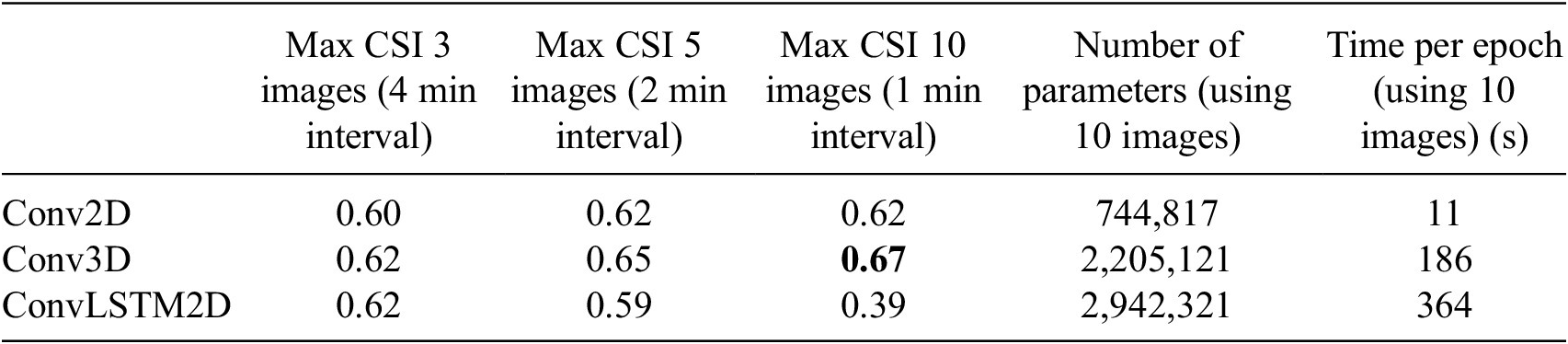
Note. Number of parameters and time per epoch for each experiment when using 10 images is also provided for comparisons. The bold value indicates the best result.
Conv3D appears to be the best solution for this application, but that is certainly not the case for all applications. The fact that the sample size is relatively small here may have put convLSTM at a disadvantage. A key takeaway is that even though convLSTM was specifically designed to extract and utilize spatiotemporal patterns, other factors, such as small sample size, may not make it the optimal solution. Generally speaking, convLSTM is a fairly complex architecture and while it may sometimes yield the best solution, it may sometimes fail miserably, as demonstrated for the 10-image dataset here. As a result, it also seems to take much more expertise to make it work. In contrast, conv3D tends to be much more robust and easy-to-use in our experience. conv2D is by far the simplest solution. It might often be less accurate, but it is fast, easy-to-use, and requires few samples, so sometimes might be the model of choice. Given that to date there are no rigorous guidelines for which convolution type to use for which application, we encourage developers, for now, to consider (and maybe try) all three convolution types, keeping the general tendencies above in mind.
5. A New Generation of Neural Networks
Convolutional neural networks brought major breakthroughs to the field of computer vision, and, a few years later, led to major breakthroughs in image-related applications in environmental science. In recent years a new generation of neural networks, attention-based neural networks, has emerged as an even more powerful framework for computer vision and is replacing traditional CNNs (i.e., CNNs that do not contain fully connected—aka dense—layers) for many applications in that field. This raises the question whether we should expect a similar trend in environmental science applications in the coming years.
Given these recent developments, we would be remiss to leave out the topic of attention-based NNs in this survey, even though there is no space here to explain these highly complex concepts in any depth. The style of this section thus differs from the previous ones in two ways:
-
1. Attention-based methods are just emerging in environmental science and it is not yet clear how prevalent these methods will become in this field. Thus this section is more looking into the future, rather than presenting past accomplishments in the field.
-
2. These concepts are very sophisticated and not easy to explain, thus we do not even attempt to explain them within the constraints of this paper, instead pointing readers to key papers. We focus here on what these new methods can do, not how they do it.
The goal of this section is thus very limited: to make environmental scientists familiar with the names of these new methods, namely attention (Vaswani et al., Reference Vaswani, Shazeer, Parmar, Uszkoreit, Jones, Gomez, Kaiser, Polosukhin, Guyon, Luxburg, Bengio, Wallach, Fergus, Vishwanathan and Garnett2017), transformer (Vaswani et al., Reference Vaswani, Shazeer, Parmar, Uszkoreit, Jones, Gomez, Kaiser, Polosukhin, Guyon, Luxburg, Bengio, Wallach, Fergus, Vishwanathan and Garnett2017), and diffusion model (Ho et al., Reference Ho, Jain and Abbeel2020), and to make them aware of the types of abilities they may add to environmental science tasks related to meteorological images and image sequences.
5.1. Core idea: Attention-based neural networks can utilize context that is not in close proximity
Attention-based neural networks were developed to meet the needs of natural language processing (NLP) to translate text from one language to another. In a translation task, a sentence is typically interpreted as a temporal sequence of words. The challenge is that each word may have multiple meanings in a language, and the correct meaning must be determined from its context, that is, from the other words in the sentence, before it can be translated correctly. Attention-based algorithms address this challenge by identifying for each word in a sentence (or paragraph or even larger context) which other words in the sentence provide highly relevant context for its meaning, that is, identify a weighting factor for all other words relative to the considered one. The weighting factors are available for all words in the sentences, not just those in close proximity of the considered word. This forms the core idea of the attention concept—a flexible way to assign context weighting to a very large number of elements, not just those in close (temporal or spatial) proximity of the considered element.
The equivalent for image processing tasks is that attention-based models allow one area of an image to be interpreted using context from all other areas of an image or image sequence. This is in contrast to purely convolutional neural networks (i.e., CNNs that do not include fully connected layers), which are only able to utilize context from the close neighborhood of a considered area. For an explanation of how the attention mechanism is implemented, that is, how attention layers can assign appropriate context weights to all words in a sentence or to all areas of an image, we refer the interested reader to Graves et al. (Reference Graves, Wayne and Danihelka2014), Bahdanau et al. (Reference Bahdanau, Cho, Bengio, Bengio and LeCun2015), and Xu et al. (Reference Xu, Ba, Kiros, Cho, Courville, Salakhudinov, Zemel and Bengio2015). The takeaway is that the attention mechanism allows one to utilize a vast spatial or temporal context, rather than being constrained to a close neighborhood.
The concept of attention has led to major breakthroughs in the abilities of AI systems for interpreting and generating text and images in other fields. For text, this is evidenced by the attention gained by ChatGPT since its release in November 2022. Similarly, for image generation three new AI-driven art tools released in 2022 demonstrate big breakthroughs: OpenAI’s Dall-E-2 (Ramesh et al., Reference Ramesh, Dhariwal, Nichol, Chu and Chen2022) and Google’s Imagen (Saharia et al., Reference Saharia, Chan, Saxena, Li, Whang, Denton, Ghasemipour, Gontijo Lopes, Karagol Ayan, Salimans, Sara Mahdavi, Gontijo Lopes, Salimans, Ho, Fleet and Norouzi2022) both generate photo-realistic images from a text description provided by a user, and Meta’s Make-A-Video (Singer et al., Reference Singer, Polyak, Hayes, Yin, An, Zhang, Hu, Yang, Ashual, Gafni, Parikh, Gupta and Taigman2022) generates 5-s video clips from a text prompt (Singer et al., Reference Singer, Polyak, Hayes, Yin, An, Zhang, Hu, Yang, Ashual, Gafni, Parikh, Gupta and Taigman2022). The abilities of these new tools were unimaginable just a couple of years ago.
Environmental science examples: Attention-based methods have already found application for precipitation mapping (Sønderby et al., Reference Sønderby, Espeholt, Heek, Dehghani, Oliver, Salimans, Agrawal, Hickey and Kalchbrenner2020; Espeholt et al., Reference Espeholt, Agrawal, Sønderby, Kumar, Heek, Bromberg, Gazen, Carver, Andrychowicz, Hickey, Bell and Kalchbrenner2022), estimating visibility due to coastal fog (Kamangir et al., Reference Kamangir, Collins, Tissot, King, Dinh, Durham and Rizzo2021), generating super-resolution imagery (Liu et al., Reference Liu, Wang, Li, Cheng, Zhang, Huang and Lu2018), wildfire estimation (Monaco et al., Reference Monaco, Greco, Farasin, Colomba, Apiletti, Garza, Cerquitelli and Baralis2021), population density estimation (Savner and Kanhangad, Reference Savner and Kanhangad2023), damage assessment (Hao et al., Reference Hao, Baireddy, Bartusiak, Konz, LaTourette, Gribbons, Chan, Delp and Comer2021), and land cover estimation (Ghosh et al., Reference Ghosh, Ravirathinam, Jia, Lin, Jin and Kumar2021; Wang and Sertel, Reference Wang and Sertel2021). Many additional examples are provided in the following section.
5.2. Use of attention for environmental imagery
In meteorology, the potential of attention-based neural networks to recognize and model patterns that extend over larger spatial and temporal distances is attractive as it may allow one to identify and model physical processes over longer time horizons. For example, important context in meteorological imagery might be provided by regions that are far away spatially, for example, due to teleconnections, that is, links between weather phenomena at large distances—typically thousands of km apart—due to large-scale air pressure and circulation patterns. Similarly, context in meteorological image sequences might be provided by images that are far away temporally, for example, to take into account the temporal evolution of a severe storm.
Attention can be integrated into NN architectures in many different ways and to different degrees. The simplest way is to take a well-established architecture, such as a CNN, and add one or more attention layers, see Section 5.2.1. On the other end of the spectrum is the development of entirely new architectures that primarily utilize the concept of attention and may no longer contain a single convolution layer, see Section 5.2.2. A third important approach is given by diffusion models which have an additional core idea but also use attention, see Section 5.2.3. Other approaches for integrating attention are beyond the scope of this survey.
5.2.1. Adding attention layers to an established NN architecture
The simplest way to start utilizing the concept of attention is to add one or more attention layers to a well-established architecture, such as a CNN. Attention layers now exist in most NN programming environments and are easy to add to an existing model as an additional layer. One of the most popular CNN architectures for meteorological imagery is the U-net architecture introduced by Ronneberger et al. (Reference Ronneberger, Fischer and Brox2015) commonly used for image-to-image translation tasks. A U-net has skip connections between its encoder and decoder layers to add high spatial resolution information from encoder layers when upsampling is conducted in the decoder layers. The Attention U-Net developed by Oktay et al. (Reference Oktay, Schlemper, Folgoc, Lee, Heinrich, Misawa, Mori, McDonagh, Hammerla, Kainz, Glocker and Rueckert2018) combines a U-net with attention layers. Specifically, it adds an attention layer in each skip connection to guide the model to focus on important features.
Environmental science examples: Attention U-nets have been used to estimate radar reflectivity (Yang et al., Reference Yang, Zhao, Xue, Sun, Li, Zhen and Lu2023), precipitation (Trebing et al., Reference Trebing, Stanczyk and Mehrkanoon2021; Gao et al., Reference Gao, Guan, Zhang, Wang and Long2022a), and cloud detection (Guo et al., Reference Guo, Cao, Liu and Gao2020) from satellite imagery. U-Nets with bidirectional LSTM and attention mechanism (Garnot and Landrieu, Reference Garnot and Landrieu2021; Ghosh et al., Reference Ghosh, Ravirathinam, Jia, Lin, Jin and Kumar2021) leverage features from time-series satellite data to identify temporal patterns of each land cover class and automate land cover classification. Wang and Sertel (Reference Wang and Sertel2021) used the attention mechanism to learn the correlations among the channels for super-resolution and object detection tasks.
5.2.2. Transformers
Transformers are the first models that can rely entirely on the concept of attention without using RNNs or convolution layers, although some choose to add convolution layers nevertheless. These models were first proposed by Vaswani et al. (Reference Vaswani, Shazeer, Parmar, Uszkoreit, Jones, Gomez, Kaiser, Polosukhin, Guyon, Luxburg, Bengio, Wallach, Fergus, Vishwanathan and Garnett2017).Footnote 3 Transformers focus on learning context from an input stream (temporal sequence) and have become the dominant architecture in the NLP domain. One of the earliest and simplest ideas to transfer the NLP approach to image analysis is to subdivide each image into small nonoverlapping patches, then treat the spatially arranged patches within an image analogous to the temporally arranged words in a sentence. This is the idea behind the VisionTransformer (ViT) introduced by Dosovitskiy et al. (Reference Dosovitskiy, Beyer, Kolesnikov, Weissenborn, Zhai, Unterthiner, Dehghani, Minderer, Heigold, Gelly, Uszkoreit and Houlsby2021), which has already been cited over 7,000 times since it appeared in 2020. Many more complex analogies and extensions have been proposed that enable the use of transformers not only for images, but also for image sequences. In contrast to the simple NNs, such as Attention U-nets, discussed in Section 5.2.1, transformers are highly complex and computationally demanding.
Environmental science examples: In 2022 the environmental science community hosted its first workshop on transformers entitled Transformers for Environmental Science (Patnala et al., Reference Patnala, Langguth, Clara Betancourt, Schneider, Schultz and Lessig2022). Specific applications include satellite time series classification (Yuan and Lin, Reference Yuan and Lin2021), change detection (Chen et al., Reference Chen, Qi and Shi2022), landcover classification (Wang et al., Reference Wang, Xing, Yin and Yang2022; Yu et al., Reference Yu, Jiang, Gao, Guan, Li, Gao, Tang, Wang, Tang and Li2022; Zhang et al., Reference Zhang, Li, Tang, Lei and Peng2022), and anomaly detection (Horváth et al., Reference Horváth, Baireddy, Hao, Montserrat and Delp2021). Gao et al. (Reference Gao, Shi, Wang, Zhu, Wang, Li and Yeung2022b) propose the use of transformers for Earth science applications by proposing an efficient space–time transformer for forecasting. Most notably, several recently proposed global weather prediction models that are purely AI-driven, such as FourCastNet (Pathak et al., Reference Pathak, Subramanian, Harrington, Raja, Chattopadhyay, Mardani, Kurth, Hall, Li, Azizzadenesheli, Hassanzadeh, Kashinath and Anandkumar2022) and Pangu-weather (Bi et al., Reference Bi, Xie, Zhang, Chen, Gu and Tian2023) are based on transformers. Transformer-based models on imagery can be further categorized as time-series transformers (Yan et al., Reference Yan, Peng, Fu, Wang and Lu2021) that are mostly applicable for forecasting, anomaly detection, and classification and work by capturing long-range dependencies from a continuous stream of meteorological images, or time-series transformers (Kazemi et al., Reference Kazemi, Goel, Eghbali, Ramanan, Sahota, Thakur, Wu, Smyth, Poupart and Brubaker2019) that work by learning time representations from the data stream or spatial transformers (Jaderberg et al., Reference Jaderberg, Simonyan, Zisserman, Kavukcuoglu, Cortes, Lawrence, Lee, Sugiyama and Garnett2015) that aim to extract the spatial features from an image.
5.2.3. Diffusion models
Generative adversarial NNs (GANs; Goodfellow et al., Reference Goodfellow, Pouget-Abadie, Mirza, Xu, Warde-Farley, Ozair, Courville, Bengio, Ghahramani, Welling, Cortes, Lawrence and Weinberger2014) and variational auto-encoders (VAEs; Kingma and Welling, Reference Kingma and Welling2013) are so-called generative (AI) models that can be used to generate detailed realistic-looking imagery. In the environmental domain GANs have been widely explored, for example, to model precipitation (Ravuri et al., Reference Ravuri, Lenc, Willson, Kangin, Lam, Mirowski, Fitzsimons, Athanassiadou, Kashem, Madge, Prudden, Mandhane, Clark, Brock, Simonyan, Hadsell, Robinson, Clancy, Arribas and Mohamed2021) and to generate remote sensing imagery (Sun et al., Reference Sun, Wang, Chang, Qi, Wang, Xiao, Zhong, Wu, Li and Sun2020; Rui et al., Reference Rui, Cao, Yuan, Kang and Song2021). Mooers et al. (Reference Mooers, Tuyls, Mandt, Pritchard and Beucler2020) use VAEs to model convection. Diffusion models (Ho et al., Reference Ho, Jain and Abbeel2020) are the first attention-based generative models and are outperforming and slowly replacing GANs and VAEs for many (but not all!) image generation tasks. Diffusion models are also a key technology behind the abilities of ChatGPT for text generation, and Dall-E-2 (Ramesh et al., Reference Ramesh, Dhariwal, Nichol, Chu and Chen2022), Imagen (Saharia et al., Reference Saharia, Chan, Saxena, Li, Whang, Denton, Ghasemipour, Gontijo Lopes, Karagol Ayan, Salimans, Sara Mahdavi, Gontijo Lopes, Salimans, Ho, Fleet and Norouzi2022), and Make-A-Video (Singer et al., Reference Singer, Polyak, Hayes, Yin, An, Zhang, Hu, Yang, Ashual, Gafni, Parikh, Gupta and Taigman2022) to generate imagery.
While diffusion models also use attention elements their core potential is based on the following idea. Diffusion models are trained by adding noise to an input image where the noise mimics a statistical diffusion process, hence the name. At each step, a small amount of noise is added, but the process is repeated several times. The NN model seeks to “undo” the damage done by the iterative diffusion process, by learning how to invert each diffusion process. Each inverse diffusion process is modeled as a statistical process with parameters learned using a NN approach—thus at execution time diffusion models are slower than standard NN models, as they have to evaluate several statistical processes. The result is a versatile tool with many potential applications in meteorology, for example, to denoise imagery, fill in missing data, or convert a low-resolution image into a super-resolution image (Google Research Brain Team, 2021). Diffusion models, since implementing statistical models, can provide probabilistic distributions at the output which is advantageous for many meteorological applications. A key disadvantage is that—in contrast to most NN models—execution is resource-intensive and relatively slow, which for some real-time applications may be a limiting factor.
Environmental science examples: Diffusion models are finally emerging in environmental science as well, for example, to generate realistic rainfall samples at high resolution, based on low-resolution simulations (Addison et al., Reference Addison, Kendon, Ravuri, Aitchison and Watson2022); to generate realistic global maps of monthly averages of temperature or precipitation in a future climate to study extreme weather events (Bassetti et al., Reference Bassetti, Hutchinson, Tebaldi and Kravitz2023); and for short-term forecasting of precipitation (Leinonen et al., Reference Leinonen, Hamann, Nerini, Germann and Franch2023). A key advantage of diffusion models for all of these applications is that diffusion models provide ensembles of solutions, which can also be used to estimate uncertainty.
6. Other Ways to Reduce the Need for Large Labeled Datasets: Self-Supervised and Transfer Learning
This section focuses on strategies to make the most of limited meteorological image data. Most meteorological data tends to be unlabeled, for example, satellite imagery usually does not come with labels that specify whether or where there is convection, or which land cover types are present. In contrast, labeled datasets come with such labels. The number of available samples along with the availability of these labels are key factors to determine which machine learning model can work best for the target application. Labeled data are often sparse in environmental science since labels are often challenging to obtain, while unlabelled data is often abundantly available. In order to fully leverage the more advanced and data-hungry models like GANs, transformers, or diffusion models, huge amounts of training samples are needed. For example, transformers tend to require huge amounts of data, and training a large transformer model is currently out of reach for many research groups due to extensive computational demands. FourcastNet (Pathak et al., Reference Pathak, Subramanian, Harrington, Raja, Chattopadhyay, Mardani, Kurth, Hall, Li, Azizzadenesheli, Hassanzadeh, Kashinath and Anandkumar2022), a transformer-based NN model for global weather forecasting, requires about 16 hr wall-clock time on 64 Nvidia A100 GPUs to train, which makes it hard for most researchers to perform hyperparameter optimization due to limited computational resources. This creates a need to utilize different types of ML techniques, including self-supervised, and transfer learning that can overcome the challenges of data quality and quantity.
Supervised Learning seeks to learn relationships between each training sample and its label, with the goal of predicting such labels during operation for new samples that come without a label. The learning is supervised in the sense that for each training sample, the model is given feedback on whether it assigned the correct label, and if not how far it was off.
Self-supervised learning utilizes information inherent in the data set as labels, often by removing some of its information, then training a NN to restore it. Examples include: taking a set of color images, removing the color, then training the NN to restore the color of the image; taking image sequences, scrambling their order, then training the NN to restore the proper order; or taking image sequences, dropping the last image of each, then asking the NN to estimate what the last image would look like given the preceding images in each sequence. Thus, the method trains against some of its own (removed) properties as output, therefore the name self-supervised. This approach allows us to train NNs without requiring labels. Bansal et al. (Reference Bansal, Bansal and Irwin2021, Reference Bansal, Bansal and Irwin2022) designed a self-supervised model to nowcast solar irradiance 15 min into the future using a combination of CNN and LSTM models on the visible channels of the GOES satellite. The key idea is that the ML model trains on the entire Continguous United States (CONUS) domain and intrinsically accounts for local geographical features without the need for external supervision or inputs. This pretrained network was then further applied on a solar specific dataset to nowcast site-specific solar power for 15 min into the future. Other applications of this are shown in (Ayush et al., Reference Ayush, Uzkent, Meng, Tanmay, Burke, Lobell and Ermon2020; Vincenzi et al., Reference Vincenzi, Porrello, Buzzega, Cipriano, Fronte, Cuccu, Ippoliti, Conte and Calderara2021).
Transfer learning has become popular in the meteorological domain to make use of relationships already learned and encoded in ML models trained for similar applications, thus also reducing the need for large labeled datasets. As the name suggests, this method involves utilizing a model trained on a task similar to the task of interest—preferably a task where a large labeled dataset is available—and transferring the extracted relationships to create a new model for the new task. If no large labeled dataset is available, self-supervised learning may be used. Gooch and Chandrasekar (Reference Gooch and Chandrasekar2020) use transfer learning for the historical discovery of weather radar imagery. They start out with a NN trained on the famous ImageNet dataset (Deng et al., Reference Deng, Dong, Socher, Li, Li and Fei-Fei2009)—a primary benchmark for object recognition research with over three million photos of objects along with object labels. They copy the lower layers which are trained to extract basic patterns from ImageNet, for example, shapes and textures, and only train the last layers of the neural network on meteorological images. The motivation is the assumption that basic patterns in meteorological imagery form a subset of basic patterns occurring in the multi-million photo collection in ImageNet. Naushad et al. (Reference Naushad, Kaur and Ghaderpour2021) showed the use of this technique on the application of classifying land use and land cover.
Overall, the strategies in this section have been used extensively for individual meteorological images and are recently emerging more prominently for image sequences as well.
7. Conclusions
In this paper, we discussed various tools to extract spatiotemporal patterns from meteorological image sequences, ranging from feature engineering to attention-based neural networks and transfer learning. In the earlier sections, we highlighted a great variety of simple, fairly transparent methods, that may be ideal for many meteorological applications—many of which are under-utilized. In the later sections, we discussed more complex and computationally demanding methods, such as transformers and diffusion models. Models utilizing these advanced concepts have shown potential to model longer-range spatiotemporal dependencies in meteorological image sequences. However, these models are also very new and the jury is still out whether their results have any significant shortcomings compared to traditional physics-based models, especially for the application of global weather forecasting.
Acknowledgments
We thank Rey Koki (CU Boulder, NOAA GSL) for emphasizing to us the huge potential of atrous convolutions for image applications. We also thank the two anonymous reviewers for their thoughtful and detailed feedback.
Author contribution
Conceptualization: All authors. Funding acquisition and supervision: K.H. and I.E. Investigation: A.S.B. and Y.L. Writing: A.S.B. wrote Section 2.2 and drafted Sections 5 and 6. Y.L. wrote Section 2.1 and contributed significantly to Section 4. K.H. wrote Section 3.1 and contributed significantly to Section 3. I.E. drafted Sections 1, 3, and 4, created Figures 2–4 and 6–11, contributed significantly to all sections, and handled most of the editing and revisions of the manuscript. All authors approved the final submitted draft.
Competing interest
The authors declare no competing interests.
Data availability statement
As a survey paper, this article does not contain any new data or code.
Ethics statement
The research meets all ethical guidelines, including adherence to the legal requirements of the study country.
Funding statement
The work by I.E.-U. and A.S.B. on this project was partially supported by the National Science Foundation under NSF AI Institute grant ICER-2019758. K.H. and A.S.B. acknowledge support by NOAA grant NA19OAR4320073.


 Open access