


Background
A suicide cluster is defined by the Center for Disease Control (CDC) as “a group of suicides or suicide attempts, or both, that occur closer in time and space than would normally be expected in a given community” (O’Carroll et al., Reference O’Carroll, Mercy and Steward1988). Unlike suicide hotspots, which are usually community-identified at public or iconic sites, clusters may span a wider geographic area and go unnoticed (be hidden) to the general population (Too et al., Reference Too, Pirkis, Milner, Bugeja and Spittal2017).
Literature has proposed three theoretical mechanisms of clusters. The first explanation is the psychology concept of suicide contagion, which functions through social learning theory (Bandura, Reference Bandura1977). The second is that people in the same area may share high-risk characteristics for suicide, such as depressed patients in an inpatient psychiatric facility (Too et al., Reference Too, Pirkis, Milner, Robinson and Spittal2019). Third, Durkheim’s classical suicide theory offers a sociological explanation hinging on social integration and regulation concepts (Durkheim, Reference Durkheim1897).
A report from the Orange County Health Care Agency (OCHCA) found that suicides were predominantly by people middle-aged, White, male, and using firearms. The report found suicide density by resident population to be greatest in coastal ZIP codes (Sanchez et al., Reference Sanchez2019; Walker, Reference Walker2019). It did not, however, examine suicide density by land mass area, which is arguably more clinically relevant when it comes to fair and equitable municipal-specific allocation of funds toward effective (Pirkis et al., Reference Pirkis, Too, Spittal, Krysinska, Robinson and Cheung2015) but often costly (Kerkhof, Reference Kerkhof2003) prevention interventions (e.g., barriers) in high-risk areas such as suicide hotspots. The OCHCA study may appear to suggest greater risk in affluent locations where there are fewer people and suicides, despite the vast majority occurring further inland in more resource-poor areas. While this type of analysis may be useful for addressing risk associated with specific types of people, such as White suburban males, it does nothing to address risk associated with specific locations and may lend itself to community bias (e.g., racial and classist). For example, this approach may lead to unfair allocation of additional prevention resources to predominantly White, resource-rich communities, abandoning locations of greater suicide numbers and risk. Analysis of suicide density by population, although fairly standard in epidemiology, fails to identify physical locations which by themselves attract suicides (e.g., through notoriety of well-known hotspots, access to means like jumping, or simply increased traffic of a downtown area) and as such, leaves out the clinical and practical relevance of suicide clusters and their effective interventions.
To the best of our knowledge, there has been only one study of clusters in Orange County (OC), assessing multiple hotspots on a university campus to date (Waalen et al., Reference Waalen, Bera and Bera2019). However, the ZIP codes wherein that study’s clusters lie are considered by the OCHCA study to be of the least suicide-dense regions by population. Therefore, it is likely that other hidden clusters exist in more suicide-dense OC regions. It is worth identifying possible hotspots, for the OCHCA failed to identify any actions at hotspots, or suicide clusters, in its report of suicide interventions (Sanchez et al., Reference Sanchez2019).
The CDC’s definition for suicide clusters offers no gold standard method for scanning for hidden clusters. A growing body of research has created multiple statistically advanced methods for detecting spatial, temporal, and spatiotemporal clusters, which require specialized software and/or trained statisticians (Cheung et al., Reference Cheung, Spittal, Williamson, Tung and Pirkis2013; Kulldorff, Reference Kulldorff1997; Tango & Takahashi, Reference Tango and Takahashi2005). Each method is imperfect in its design and, most importantly, is not easily applied by the average community stakeholders who the CDC ultimately holds responsible for suicide prevention (Hill et al., Reference Hill, Too, Spittal and Robinson2020; O’Carroll et al., Reference O’Carroll, Mercy and Steward1988). Furthermore, these methods’ emphasis on statistical significance requires comparisons with unrelated, outside populations, lacks sensitivity, and may not apply to community-identified clusters (Boyce, Reference Boyce2011; O’Carroll & Mercy, Reference O’Carroll and Mercy1990). This presents a major barrier to ongoing, real-time cluster detection required for necessary targeted interventions in the midst of our growing national suicide epidemic. “There is no reason to believe that all suicide clusters will inevitably come to the attention of health authorities through passive identification by groups in the community”… and… “early intervention might provide the best chance for minimizing the hypothesized contagious effect of suicide” (O’Carroll & Mercy, Reference O’Carroll and Mercy1990). As such, the community is in urgent need of an accessible, operational definition and efficient modality to detect and monitor clusters in ongoing, real time.
The goal of this study is threefold: (a) test via face validity, a simple method using readily accessible household software to identify suicide clusters; (b) identify spatial and temporal suicide clusters in OC, and (c) examine possible mechanisms for these clusters, including suicide contagion (via relationship between temporal and spatial clusters), shared characteristics, and danger of location.
Materials and methods
Study design and data collection
The university IRB exempted this study from full review. Our design consisted of a population-based retrospective study of completed suicides in Orange Country from 2014 to 2019 based on data from the OC Sheriff’s Department Coroner Division. These data were Coroner-determined and confirmed. For each suicide, data obtained included death date and time; gender (listed by sex), age (which we grouped into 10-year cohorts), and race of individuals; attempt means/mode; event address and place (e.g., hotel, freeway, and beach); and death address and place. In certain cases (e.g., ocean drowning), data described locations in terms of nearest location. We identified 618 total suicides. We individually mapped, rather than aggregated, suicide locations using Microsoft Excel and its Excel 3D Maps system.
Spatial clusters
From event locations, Excel 3D Maps generated heat maps showing suicide densities per 2.5 km viewing diameter region (3.9 km2 area). Its spatial interface is Bing Maps. The diameter was measured with Google Maps’ measuring tool with landmarks for reference. We arbitrarily defined a meaningful threshold of suicide density per area of 1.39/km2 defined as the 95th percentile of a normal logarithmic scale distribution of suicide density per area in each ZIP Code Tabulated Area (ZCTA) cumulated from all years. Four outliers in this distribution were not included. We examined each data point for location accuracy. If there were any locations Excel 3D Maps could not recognize, we examined and manually altered the address in question for accurate plotting. We subsumed suicides of five Zip codes with no corresponding ZCTA under the surrounding Zip code. We removed three ZIP codes whose suicide attempts did not, but whose corresponding deaths did, occur in OC. We color-coded map densities on a scale ranging from blue (0 suicide events) to red (≥1.39/km2). We identified red regions as potential “hotspots” and examined the associated suicide victim (e.g., race and sex) and observed map (e.g., type of place and features) data to infer possible associations with suicide clusters.
Temporal clusters
We defined a meaningful threshold of 33.9 suicides per yearly quarter as the 95th percentile of a normal distribution of suicide density per quarter using 24 three-month quarters between 2014 and 2019. We created a list of 70 potential “quarters” of three consecutive calendar months and identified the quarters exceeding the previously defined meaningful threshold of suicide density. We generated via Microsoft Excel a one-dimensional temporal map and labeled 3-month meaningful cluster(s). We then cross-referenced the suicides of these temporal clusters with those of spatial clusters to look for evidence of contagion at spatial clusters.
Statistics
No formal cluster analysis was done. Clusters were described as above and identified manually by color on a map of OC. Associations with known geographic locations were identified manually.
Results
Data demographics
Racial diversity ranged from 69% (425) White, 17% (103) Hispanic, 12% (72) Asian, and 3% (17) Black to 0% (1) unknown. Sex split into 83% (510) Male and 17% (108) Female. Age diversity ranged from 4% (24) 10–19, 20% (125) 20–29, 18% (112) 30–39, 15% (90) 40–49, 20% (121) 50–59, 15% (95) 60–69, 6% (34) 70–79, and 2% (12) 80–89 to 1% (5) 90–99. Mode ranged from 25% Asphyxia (157), 22% (139) Gunshot, 15% (91) Overdose, 14% (87) Fall, 7% (44) Vehicular-Traffic, 6% (38) Train, 3% (17) Cutting/Stabbing, 3% (21) Drowning, 1% (8) Fire, 1% (8) Blunt Force Trauma, 1% (4) Vehicular-Private Property, 0% (2) Other, and 0% (1) Religious Objections, to 0% (1) Broken Neck (via hanging).
Spatial clusters
From all 618 total suicides, we identified 21 meaningful (greater than 1.39/km2) spatial clusters throughout OC for years 2014–2019, labeled as “All Suicide” (AS) clusters (Figure 1). By visual inspection, 31% of all suicides (192) appear to be in clusters. Of clusters (Table 1), 81% (17/21) included major transportation lines, 62% (13/21) included major tourist attractions or recreational parks, 48% (10/21) included educational centers or educational housing, 33% (7/21) included mobile home parks, 33% (7/21) included major bodies of water, 29% (6/21) included two-star hotels, 19% (4/21) contained medical centers, 19% (4/21) included downtown areas, 10% (2/21) included cemeteries, 5% (1/21) included an airport, and 5% (1/21) included LGBT Centers.

Figure 1. Meaningful spatial clusters of all suicides in Orange County (OC) years 2014–2019 (numbered). Out of 618 total suicides, we identified 21 meaningful spatial clusters (numbered here) throughout OC for the years 2014–2019. We arbitrarily defined a meaningful threshold of suicide density per area of 1.39/km2 defined as the 95th percentile of a normal logarithmic scale distribution of suicide density per area in each ZIP Code Tabulated Area cumulated from all years. We color-coded map densities on a scale ranging from blue (0 suicide events) to red (≥1.39/km2). We identified red regions as potential “hotspots.”
Table 1. Frequency of features per cluster
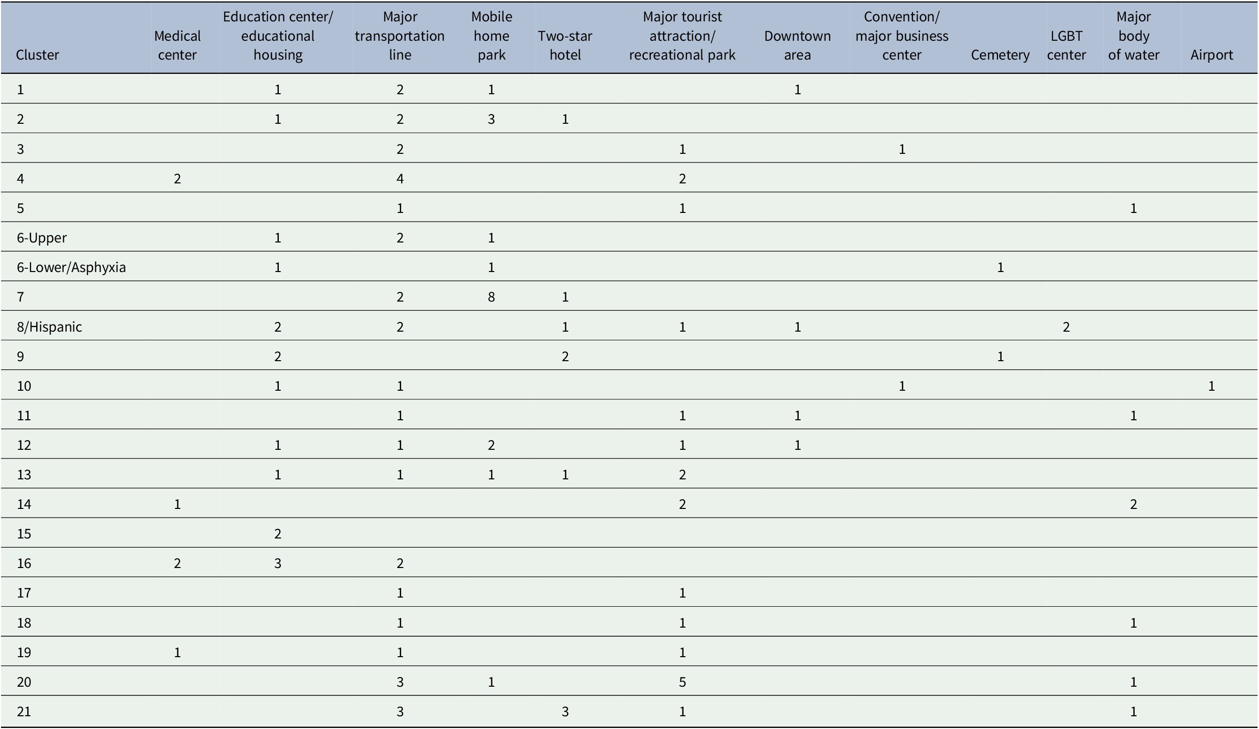
Note. Depicted here are the numbers of features observed in each AS cluster. We defined education centers as high schools, colleges, or universities, educational housing as university campus housing, and major transportation lines as rail lines, freeways, highways, and major streets. Of these clusters, 81% (17/21) included major transportation lines, 62% (13/21) included major tourist attractions or recreational parks, 48% (10/21) included educational centers or educational housing, 33% (7/21) included mobile home parks, 33% (7/21) included major bodies of water, 29% (6/21) included two-star hotels, 19% (4/21) contained medical centers, 19% (4/21) included downtown areas, 10% (2/21) included cemeteries, 5% (1/21) included an airport, and 5% (1/21) included LGBT Centers.
No age cohort produced meaningful spatial clusters (Figure 2). Hispanic (Figure 2a) and White (Figure 2b) were the only races with meaningful spatial clusters. The one Hispanic cluster coincided with AS cluster 8 and a Male Sex cluster. This was located in a Latino-predominant city and included its downtown area, two rail lines, the city zoo, the OC LGBT Pride office, the OC LGBT Center, and a two-star hotel. It was sandwiched between two high schools.
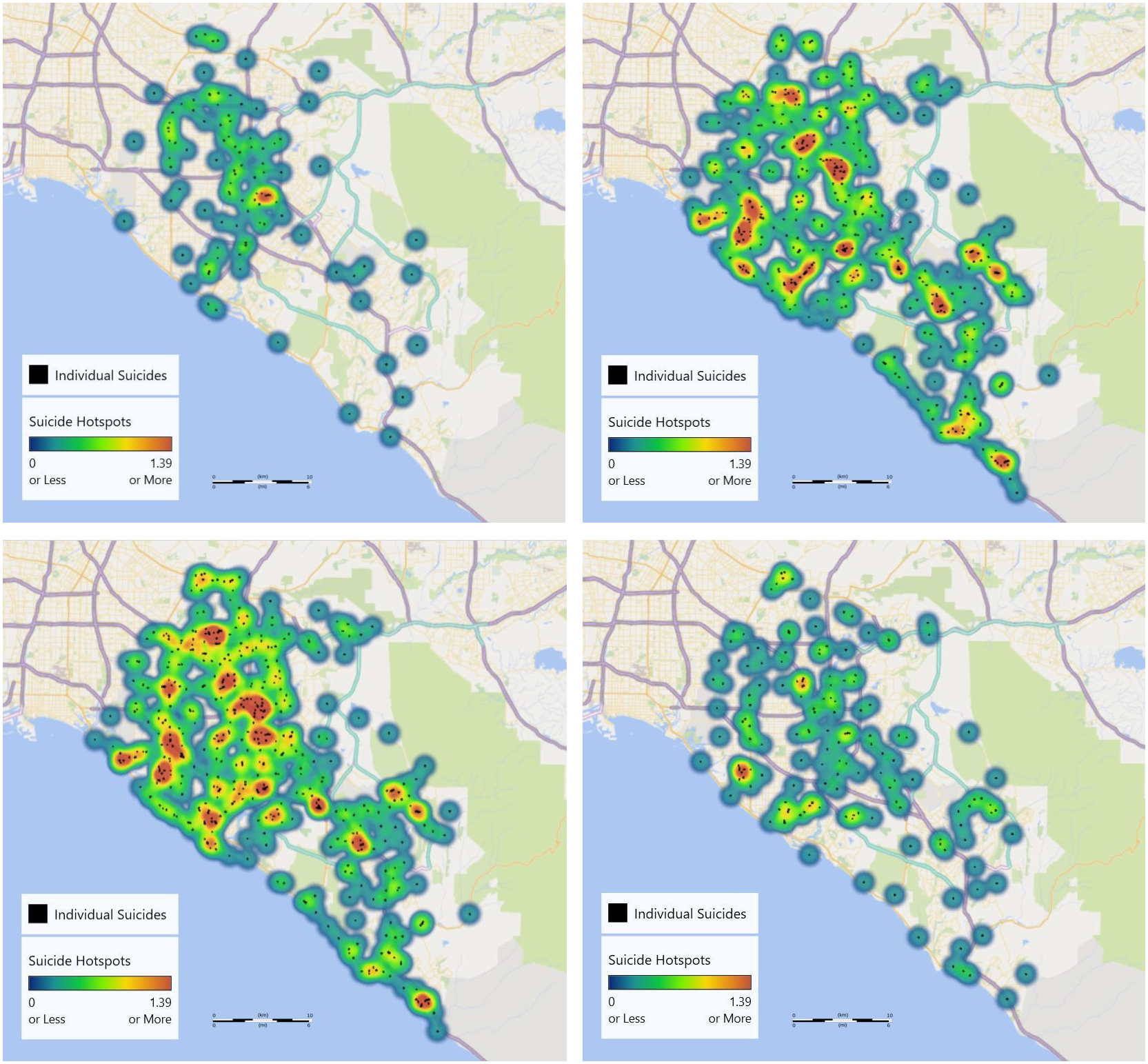
Figure 2. Meaningful spatial clusters of suicides by shared characteristics in Orange County (OC), years 2014– 2019. Using our meaningful threshold of suicide density per area, 1.39 km−2, meaningful clusters (depicted in red) of suicides with the following shared characteristics are identified. A) Hispanics in OC, years 2014–2019: one Hispanic cluster was identified. This coincided with AS cluster 8 and a Male Sex cluster. It was located in a Latino-predominant city and included its downtown area, two rail lines, the city zoo, the OC LGBT Pride office, the OC LGBT Center, and a two-star hotel. It was sandwiched between two high schools. B) Whites in OC, years 2014–2019: 15 White clusters were identified which coincided with AS clusters #1, #3, #4–6, #10–13, and #16–21. All White clusters but #11, #13, and #20 coincide with Male clusters. C) Males in OC, years 2014–2019: 17 Male clusters were identified, which coincided with AS clusters #1–8, #10, #12, #14–19, #21, and the Hispanic cluster. All Male clusters but #2, #7, #8, #14, and #15 coincided with White clusters. Female sex did not produce any meaningful clusters. D) Asphyxia in OC, years 2014–2019: Asphyxia was the only mode to produce a meaningful cluster. This coincided with the lower (southern) portion of AS cluster 6, which was dumbbell-shaped. Hanging constituted 87% (136/157) of asphyxia suicides. Other types included suffocation and carbon monoxide poisoning.
White race (15) and Male sex (17) (Figure 2c) produced the highest number of meaningful clusters. White clusters coincided with AS clusters #1, #3, #4–6, #10–13, and #16–21. All White clusters but #11, #13, and #20 coincide with Male clusters. Male clusters coincided with AS clusters #1–8, #10, #12, #14–19, #21, and the Hispanic cluster. All Male clusters but #2, #7, #8, #14, and #15 coincided with White clusters.
Female sex did not produce any meaningful clusters. Asphyxia was the only mode to produce a meaningful cluster (Figure 2d). This coincided with the lower (southern) portion of AS cluster 6, which was dumbbell-shaped. Hanging constituted 87% (136/157) of asphyxia suicides. Other types included suffocation and carbon monoxide poisoning. While suicide by train did not produce meaningful two-dimensional clusters, suicides clustered in a clearly identifiable linear form along two major rail lines, particularly at their junction passing by eight medical centers and a nationally recognized theme park (Figure 3). These corresponded with AS clusters #1, #3, #4, #8, #20, and #21. All but #8 coincide with White clusters. All but #20 coincide with Male clusters.
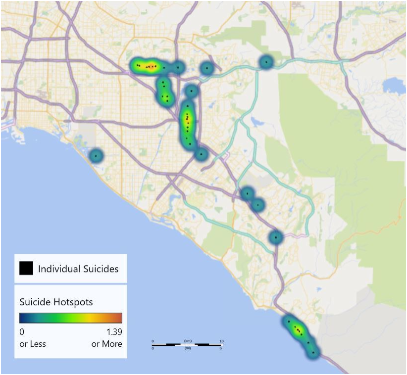
Figure 3. Non-“meaningful” spatial suicide clusters of interest of suicides by train in Orange County years 2014–2019. While suicide by train did not produce meaningful two-dimensional clusters, suicides clustered in clearly identifiable linear form along two major rail lines, particularly at their junction passing by eight medical centers and a nationally recognized theme park. These corresponded with AS clusters #1, #3, #4, #8, #20, and #21. All but #8 coincide with White clusters. All but #20 coincide with Male clusters.
Of note, most of cluster 1’s suicides were near the rail line, which cut across the cluster center, or one of the two freeways. More than half of cluster 2 suicides centered around the two-star hotel and one of the mobile home parks. cluster 3 included a nationally recognized theme park. cluster 7 included eight mobile home parks. cluster 15 predominantly consisted of a major university and its campus housing. cluster 20 contained five major tourist attractions or recreational parks (Table 1).
Temporal clusters
Of 70 possible 3-month quarters, we identified one temporal cluster (Figure 4). This was July to September 2017. With 36 suicides, it yielded an average of 12 per month. Of those, 89% (32) were male, 63% (23) were White, 17% (6) were Hispanic, 11% (4) were Asian, and 8% (3) were Black. Of modes, 28% (10) were Asphyxia, 6% (2) were Drowning, 17% (6) were Fall, 17% (6) were Gunshot, 14% (5) were Vehicular-Traffic, 14% (5) were Overdose, 3% (1) were Train, and 3% (1) were Cutting/Stabbing. As these were evenly spaced across OC, we could not identify any temporospatial clusters. Numbers per city ranged from one (13 cities) to five (1 city). Two of similar age but distinct race and mode occurred at opposite sides of a freeway intersection in spatial cluster 13.
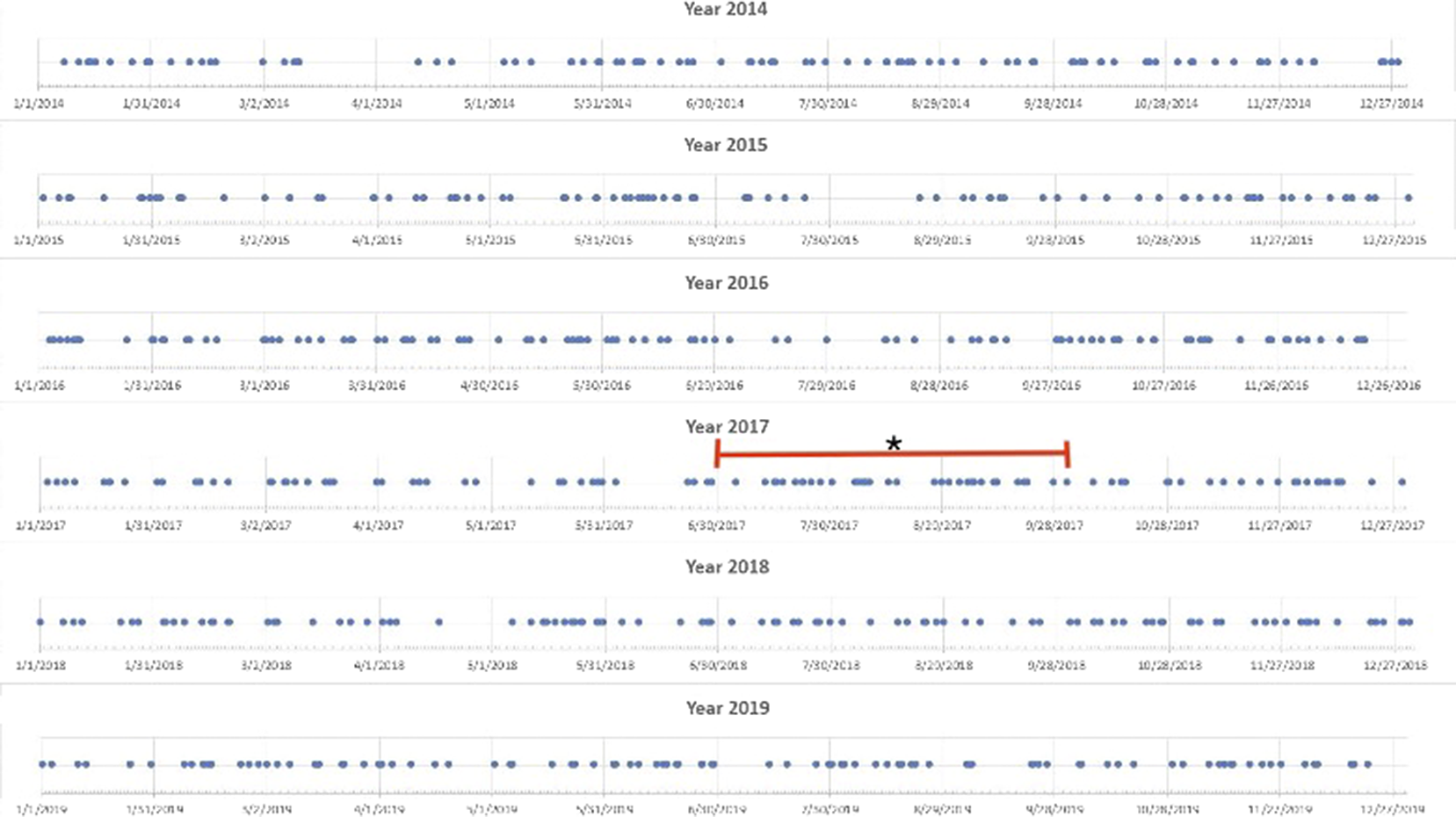
Figure 4. Meaningful temporal clusters in Orange County (OC) years 2014–2019. Using a meaningful threshold temporal density of 33.9 suicides per yearly quarter, we identified one 3-month-long temporal cluster. This was July to September 2017. As these suicides appear to have been evenly spaced across OC, we could not identify any temporospatial clusters.
Discussion
Through this study, we achieved a simple, novel method of identifying clinically meaningful clusters using the commonly available household computer program, Excel and its 3D Maps. To the best of our knowledge, we are the first to demonstrate the utility and face validity of this readily available system for identifying meaningful suicide clusters, which has the potential to allow communities to more easily recognize and address suicide hotspots. We identified 21 AS “All Suicides” spatial clusters and clusters of White, Hispanic, Male, and Asphyxia categories. White, Hispanic, Male, and Asphyxia cases were more common and thus more likely to yield meaningful thresholds of suicide area densities. All these subgroup clusters coincided within the AS clusters, giving validity to their meaning as suicide hotspots. Upon examination of the entirety of OC, only one temporal suicide cluster was found.
Three possible explanations for clusters exist: (a) suicide contagion (which may be supported by temporal clusters), (b) shared characteristics of people completing suicide within clusters, and (c) characteristics of the area that predispose to suicide.
Our temporal cluster did not localize to any part of OC. Internal or external forces may have affected all of OC (e.g., seasonal [Partonen et al., Reference Partonen, Haukka, Nevanlinna and Lönnqvist2004; Shapiro, Reference Shapiro2019], social [Bridge et al., Reference Bridge, Greenhouse, Ruch, Stevens, Ackerman, Sheftall, Horowitz, Kelleher and Campo2020], political [The Trevor Project, 2016; The Trevor Project et al., Reference Lunn and Daniel2017], and random chance). Given our temporal cluster displayed diversity in its locations, sex, race, age, and mode, we found no evidence of internal suicide contagion.
Shared characteristics in our spatial clusters provided face validity to our method and support the idea of shared characteristics among people and areas predisposing to clusters. These included high schools, colleges, and universities. Out of OC’s 28 colleges (Orange County, 2020b) and universities and nine high schools (U.S. News, 2020), we found 43% (16) in clusters. Surprisingly, in attempting to relate this to the generally higher risk of suicide among teens and young adults, we found relatively few suicides in the ages of 10–19 though stable frequency distribution through the ages of 20–69. These numbers actually match the rates among different age groups nationwide in 2018 (AFSP, 2020), the year of many of these suicides. Due to low death rates among teenagers in this population, the high school proximity to a cluster may have posed as less of a suicide risk factor compared to college/university proximity. Perhaps these results are due to underreporting of teen deaths or protective factors instituted within these particular high schools, such as suicide prevention campaigns, although this is purely speculation. Despite the association between adolescents and young adults with clusters (Gould & Lake, Reference Gould and Lake2013), we could identify no clusters by any age groups. This may be due to our viewing diameter or differences in data collection. cluster 15 appeared to underrepresent the suicide number compared with that reported by its campus police department over the same time period (Waalen et al., Reference Waalen, Bera and Bera2019). Age groups among those aged 20–59 did appear to track along areas of higher suicide density, possibly because they constituted the majority of suicides.
Other common characteristics included mobile home parks, possibly due to socioeconomic stressors, although this is purely speculative. Preexisting addiction problems (Romney & Hua, Reference Romney and Hua1995) which can increase suicidality through substance use could have led to increased socioeconomic stressors and increased likelihood of living in a mobile home park. While we found only 7% of OC’s 245 mobile home parks (Orange County, 2020a) in clusters, not all mobile home parks may be clustered in such a way as to predispose to suicide clusters. The relevance of mobile home park presence may lie in their proximity to one another, as was seen in cluster 7, whose standout feature was eight mobile home parks. Similar explanations can be had for two-star hotels. Medical centers were common, likely due to higher presence of psychiatric patients. LGBT Pride Office and OC LGBT Center were present in cluster 8, the Hispanic cluster. LGBT population concentration around these service sites may explain higher suicide numbers, due to higher risk (The Trevor Project, 2021). Cemeteries may prime the suicidal person on the notions of death, dying, and glorification of death through acts of remembrance and paying of respects done at cemeteries. Freeways and rail lines may contribute to increased suicide risk by area both through increased people traffic as well as via increased availability of vehicular and train collision suicide modes. Similarly other area characteristics of high people traffic, such as convention centers, theme parks, beaches, tourist attractions, and airports, may predispose to higher suicide numbers.
We found examining suicide risk by area instead of by population gave very different results than OCHCA’s study (Sanchez et al., Reference Sanchez2019). Unlike their study which found risk per population greater in the affluent ZIP codes along the coast, ours found greater risk per area in areas further inland, with lower economic resources (Orange County Register, 2008), and of high population density (Brinkhoff, Reference Brinkhoff2021). Similar to theirs which found greater risk among Whites and Males, ours found spatial clusters presenting the greatest risk for Whites and Males. However, the Hispanic cluster, cluster 8, represented a never-before identified area showing risk for Hispanic people as well. This can be explained by a higher population density. Perhaps it also represents a higher risk of being Male, Hispanic, and LGBT, given the Hispanic cluster’s LGBT community centers and coincidence with the Male cluster. Unfortunately, LGBT identity is not routinely recorded in county data, but it would be interesting to compare risk of such identity intersection in places such as Los Angeles, which has several LGBT Centers and Hispanic-predominant neighborhoods. This method provides a more pragmatic way to focus preventive resources into culturally specific areas with more suicide.
Furthermore, there were differences between the OCHCA study and ours, possibly related to differences in data collection. We used free, readily accessible data from the OC Coroner’s office, because bureaucratic and financial barriers impeded our use of the same data sources as OCHCA’s study, the State of California’s Department of Public Health Death Statistical Master File and Vital Records Business Intelligence System. We also included an additional year, 2019, in our study. While OCHCA’s study found that suicides were primarily conducted via firearms, this study found most suicides were carried out through Asphyxia, which is not explained by the additional study year, 2019. Spatial cluster 6 presented the greatest risk for asphyxia. The vast majority of these suicides were by hanging, specifically. These may coincide within a hidden temporal cluster not identified via our parameters, thus representing contagion. Lastly, while the prior study found greatest suicide numbers among the middle-aged, this study found equal or greater numbers from those in their 20s (20%) than from those in their 40s (18%) or 50s (20%).
We propose this alternative method, for its accessibility and ease of use, to identify and monitor potentially overlooked meaningful clusters, at-risk features, and possible targets of intervention. Possible interventions specific to OC are mental health resources and suicide prevention campaigns that target cluster sites as well as their shared characteristics such as high schools, colleges, and universities; mobile home parks; areas of increased people traffic such as trains, highways, downtown areas, convention centers, beach and theme parks, tourist attractions, business complexes, airports, and educational campuses; and medical centers. We warn against the use of suicide by ZIP code population data to determine allocation of suicide prevention resources. We recommend focusing the allocation of said resources to the regions with the greatest number of suicides, rather than to the ZIP code populations with the greatest risk of suicide, in order to have the greatest impact on suicide prevention. One caveat would be that consideration must be made regarding cultural barriers in providing resources to any high-risk population.
Limitations and future work
“The sensitivity with which attempted suicides are identified may be much greater during a community-identified cluster of completed suicides than otherwise…. Statistically verified clustering of suicide attempts [alone] tells us little about the statistical probability of an associated community-identified cluster of completed suicides.” (O’Carroll & Mercy, Reference O’Carroll and Mercy1990). Even statistically significant clusters alone do not prove contagion (Suicide Contagion: A Systematic Review of Definitions and Research Utility). While our identification of cluster 15, corresponding with a community-identified temporospatial hotspot studied elsewhere (Waalen et al., Reference Waalen, Bera and Bera2019), does provide face validity to our method, it would be inappropriate to rule out a cluster due to lack of statistical significance, particularly if the community has identified it first.
Further limitations of this study include observer bias affecting which shared characteristics of clusters were identified. Future studies should aim to account for such bias with a more structured approach. While the mode of Train did not show any hotspots, this may be due to its linear shape, which is not as easily captured by our circular model of capturing suicide density by area. Other methods of identifying clusters along linear pathways should be considered (Too et al., Reference Too, Pirkis, Milner, Bugeja and Spittal2017). This study was limited by the magnification parameters at which we searched for clusters. The magnification we chose was somewhat arbitrary. Examination of spatial and temporal clusters at different viewing diameters may be of additional utility. For example, cluster 15’s suicides did not show up in the temporal cluster we identified when looking on the scale of OC as a whole. By studying individual clusters such as cluster 15 on their own, however, it may be possible to identify temporal clusters on preset time blocks ranging from weeks to months to years.
On first inspection, it seems strange that 31 and 7% of suicides were located in spatial and temporal clusters, respectively, defined to have a density threshold of the 95th percentile. This is both a limitation and advantage of the study method. Depending on viewing diameter, clusters may aggregate, merging into others and potentially leading to overrepresentation of cluster size. For future use, this may be easily corrected by altering the viewing diameter. At the same time, heat map technology transcends the limitations of other scan statistics, which often operate only in either circular/elliptical or linear form, allowing for irregular shapes and interesting connections between locations of relevance, such as circular centers and linear rail and roadways.
For simplicity, we used ZCTA distribution to define the 95th percentile threshold suicide density as opposed to a census block group. Locations came with ZIP codes, which made it easy to use ZCTA’s. This presented its own room for error, however, as ZCTA’s, like census block groups, come in varying shapes and sizes. Had an overlying grid system been as easily accessible to the average layman, we would have used it to ensure uniform areas from which to draw our distribution of densities.
Another study limitation is the Coroner’s data supplied addresses (or nearest addresses) of events, not exact global positioning system coordinates. Only 8% appeared to have involved a vehicle, suggesting several near roads and railways occurred indoors. Upon closer inspection, a fair number appear to have been in parked automobiles and hotels. An important aim of a future study might be to examine more closely characteristics of exact locations along roads and railways possibly making them more dangerous for suicide.
With any statistical study, there is the potential for random error. For simplicity, we chose not to use an outside control population because every population is unique. Instead, we examined the same population over the course of several years. It is possible that certain clusters may appear randomly as part of a normal distribution without relationship to high-risk locations or time periods. Regardless, it is always important to monitor any clusters in ongoing real time to monitor for persistent or recurrent patterns (Waalen et al., Reference Waalen, Bera and Bera2019), which is why a widely and readily accessible method such as ours is so important. In this study, we valued ease of use over specificity with the assumption that increased access would promote much needed long-term cluster monitoring.
Conclusions
Through this proof of principle study, we achieved a simple, novel method of identifying suicide clusters using the commonly available household computer program, Excel. Shared characteristics in these spatial clusters provided face validity to our method and support the idea of shared characteristics among people and areas predisposing to clusters. We found that examining suicide risk by area instead of by population gave very different results than OCHCA’s study. We propose this alternative method, for its accessibility and ease of use, to identify and monitor in real-time potentially overlooked meaningful geographic or temporal clusters, at-risk features, and possible targets of intervention.
Acknowledgment
We give special thanks to Hollis Krug, MD, for language and technical editing.
Open peer review
To view the open peer review materials for this article, please visit http://doi.org/10.1017/exp.2023.2.
Data availability statement
Given the sensitivity of information, data and analysis may be available on request only.
Funding statement
This research received no specific grant from any funding agency, commercial, or not-for-profit sectors.
Conflict of interest
The authors declare none.


 Open access
Comments
Comments to the Author: The paper deals with an extremely interesting topic and, as can be inferred from the analysis produced, presents itself as a first attempt to make a very uneven literature organic. In detail, the paper claims to present a real-time cluster detection required for necessary targeted interventions in the midst of our growing national suicide epidemic.
The problem addressed and the solution proposed look interesting, the paper is well structured but not well organized. It could be useful to provide a thoughtful discussion of how the paper serves as a foundation for future research with a dedicated section.
In particular, the introduction should give an overall review of the paper (including contributions, approach, results, advantages) while a "related work" section clearly outlines the perspective on this field with the discussion of all the references cited. In the same related work section, the authors can report other references in which these algorithms are applied. This could prevent a clear understanding of what should be the contributions of this paper, starting from its novelties.
The discussions should provide more explanations and particulars of the underlying meaning of this research, noting possible implications in other areas of study, and exploring possible improvements.
The English is correct, but more attention could be addressed to text errors and stylistic inaccuracies.
The section Conclusion should be expanded and improved by introducing more explanations and particulars of the underlying meaning of this research, noting possible implications in other areas of study, as well as results should be mainly discussed in relation to previous researches.