


1. Introduction
In response to the coronavirus disease 2019 (COVID-19) pandemic, a sequence of federal financial aid packages (i.e., the Coronavirus Aid, Relief, and Economic Security [CARES] Act, the Coronavirus Response and Relief Supplemental Appropriations [CRRSA] Act, and the American Rescue Plan [ARP] Act) were launched by the U.S. government in an effort to protect consumers and businesses and to stimulate the economy.Footnote 1 From March 2020 through 2021, many U.S. households received financial assistance in the form of economic impact payments (i.e., stimulus payments), additional unemployment benefits, and child tax credits, among others (H.R.133—116th Congress (2019-2020): Consolidated Appropriations Act, 2021, 2020; H.R.748—116th Congress (2019-2020): CARES Act, 2020; H.R.1319—117th Congress (2021-2022): American Rescue Plan Act of 2021, 2021; Schild and Garner, Reference Schild and Garner2021). These stimulus bills have been among the largest aid packages in U.S. history (Boccia and Bogie, Reference Boccia and Bogie2020; Brewster, Reference Brewster2020), inspiring numerous assessments of their effectiveness in spurring economic activity and measuring their impact on consumer behavior. Such assessments include Baker et al. (Reference Baker, Farrokhnia, Meyer, Pagel and Yannelis2020), Chetty et al. (Reference Chetty, Friedman, Hendren and Stepner2020), Coibion, Gorodnichenko, and Weber (Reference Coibion, Gorodnichenko and Weber2020), and Schild and Garner (Reference Schild and Garner2021), to name but a few. However, there is a lack of refereed research evaluating the extent to which each federal aid package influenced consumer spending behavior in food retail and foodservice outlets while controlling for important demographic characteristics that vary across consumers.
The U.S. food sector, in particular, experienced substantial change in spending patterns as residents resorted to “panic buying” at the onset of the pandemic (Altstedter and Hong, Reference Altstedter and Hong2020; Kassas and Nayga Jr., Reference Kassas and Nayga2021; O’Connell et al., Reference O’Connell, de Paula and Smith2021), and as food demand shifted away from foodservice and into retail (Chenarides et al., Reference Chenarides, Manfredo and Richards2021; Deconinck, Avery, and Jackson, Reference Deconinck, Avery and Jackson2020; Hayes et al., Reference Hayes, Schulz, Hart and Jacobs2021; Hobbs, Reference Hobbs2020; Weersink et al., Reference Weersink, von Massow, Bannon, Ifft, Maples, McEwan and McKendree2021; Zeballos and Dong, Reference Zeballos and Dong2021). From USDA Economic Research Service (2022) estimates, February to March of 2020 saw national food-at-home (FAH) expenditures increase from 65 to 81.8 billion dollars, or 26%. By comparison, national FAH expenditures rose only 12% from February to March of 2019 (USDA Economic Research Service, 2022). Conversely, national food-away-from-home (FAFH) expenditures fell from 79.3 billion dollars in February 2020 to 41.8 billion dollars by April 2020, or a 47% reduction in just two months’ time (USDA Economic Research Service, 2022). On net, total national food sales declined by 32.1 billion dollars, or 22%, from March to April of 2020 and did not recover to pre-pandemic levels until July of the same year (USDA Economic Research Service, 2022).
COVID-19 substantially impacted the vital U.S. food industry, with economic losses at the onset of the pandemic measured in tens of billions of dollars per USDA statistics discussed above. Federal efforts to spur economic activity and protect consumers and vital industries may have thwarted even larger adverse impacts by enabling, or perhaps incentivizing, U.S. consumers to spend on food. However, prior studies have not accessed this enabling or incentivizing of food purchases across food outlet types and for each wave of federal spending. Given the magnitude of impact COVID-19 had on the U.S. food industry, the historically large amount of federal money provided to the public during the pandemic, and there being multiple payments made available to U.S. consumers, a richer assessment of governmental policy and its impact on the U.S. food industry is warranted. This research provides such an assessment, centering around two primary research questions. First, did the economic impact payments (EIPs) provided through the CARES, CRRSA, and ARP Acts incentivize or enable U.S. consumers to purchase food away from home during the human health and economic disruption? Second, were larger payments associated with increased spending in both FAH and FAFH outlets and did that association differ between the three payments?
To answer the stated research questions, a Tobit model is estimated – separately for each of the three federal payments and using household-level survey data – to determine the association between the EIPs and survey respondents’ household FAH spending while accounting for censored expenditures. A selection model is also estimated, separately for each of the three payments, to determine the association between the EIPs and the probability of a household having spent on FAFH. The association between the payments and household FAFH expenditures is then quantified, conditional on a household having spent on FAFH. Estimating the censored FAH model and FAFH selection model separately for each stimulus package and allowing the level of federal financial aid to vary across models (reflecting the payment qualification specifications of each aid package) enables assessment of how associations between the EIPs and household food expenditures may have changed as each aid package was implemented.
Rather than use national estimates of household food expenditures as provided by the U.S. Department of Agriculture (USDA) or scanner-based data as utilized by Marchesi and McLaughlin (Reference Marchesi and McLaughlin2022) and McLaughlin et al. (Reference McLaughlin, Stevens, Dong, Chelius, Marchesi and MacLachlan2022), this study uses household-level food expenditure data from the Meat Demand Monitor (MDM) online survey (AgManager.info, 2022b). Federal COVID-19 aid, consumer demographics, and spending behavior vary significantly across households. Using disaggregated MDM survey data allows for a refined estimation of food expenditures for households of differing size, income, EIP receipt, and other factors. Additionally, the majority of prior survey-based studies on consumer spending during the COVID-19 pandemic generally evaluated CARES Act EIPs only. The CRRSA and ARP Acts also provided direct payments, which have been largely unexamined in empirical work on consumer spending reactions during COVID-19. We add to previous work by estimating the associations between all three EIPs and household FAH and FAFH expenditures – all while controlling for important household characteristics unavailable through nationally aggregated or scanner-based data sources. To our knowledge, no other study has evaluated heterogeneity of EIP spending response in the U.S. food industry across food outlets and federal aid packages.
Beyond valuable information on the determinants of household food expenditures, this study provides food manufacturers, retailers, and foodservice an understanding of consumer spending response on food with an influx of additional income (i.e., EIPs in this instance) and how that response varies across food outlet types. Further, policymakers are provided an understanding of how COVID-19-related fiscal policy impacted a vital U.S. industry. That is, the effectiveness of future governmental efforts to maintain economic activity or protect crucial industries during periods of distress can be better gauged by the results of our analysis. It is our hope that this work, and the conglomerate of similar research on other industries, can guide governmental decision makers in crafting effective policy in the instance of another major economic disruption. In that light, the remainder of the study is as follows. First, a review of relevant literature is provided, followed by a summary of utilized data and methods. We then discuss the results of our analysis, overview limitations of our work, and conclude with key implications.
2. Literature review
A host of research has been conducted following the onset of the COVID-19 pandemic assessing U.S. consumers’ use of EIPs. Summarized in this section are relevant efforts that have made use of survey-based or other disaggregated, consumer-level data on EIP receipt and food expenditures. Though valuable assessments of the impacts of federal aid on economic activity, these studies were either conducted before distribution of the second (CRRSA Act) and third (ARP Act) payments or had a primary focus on sectors other than food retail and foodservice – of key interest for our research.
Baker et al. (Reference Baker, Farrokhnia, Meyer, Pagel and Yannelis2020) analyzed household CARES payment spending response using transaction-level data from SaverLife, a nonprofit financial technology. Income levels and liquidity of wealth were important determinants of households’ marginal propensity to consume CARES Act EIPs, suggesting household characteristics should be controlled for in our assessment of food expenditures. Spending on food after receiving the payments was estimated to be larger than previous economic stimulus programs of 2001 and 2008, which lends credence to hypotheses that associations between EIPs and food expenditures may have changed between the three COVID-19-related aid packages. Relative increases in payments on rent, mortgages, and other debt were also experienced compared to the 2001 and 2008 periods, making the direct cash payments less effective in stimulating aggregate consumption.
Using data from several private companies and constructing indices of transaction-level consumer spending, employment, and other metrics, Chetty et al. (Reference Chetty, Friedman, Hendren and Stepner2020) estimated the causal effect of CARES Act EIPs on consumer spending using a regression discontinuity design. Stimulus payments resulted in increased spending, especially among lower-income households, but little went toward the businesses most affected by COVID-19-related shutdowns. Further investigating the composition of goods bought using CARES Act EIPs, the authors found that spending on durable goods rose by 21 percentage points following receipt of payments while spending on in-person services rose by only 7 percentage points. Results from Chetty et al. (Reference Chetty, Friedman, Hendren and Stepner2020) showing differences in EIP spending response across goods and business types suggest that an important disparity may exist between FAH and FAFH spending upon receipt of a payment.
A host of surveys have been distributed to gauge how consumers spent CARES Act EIPs (Akana, Reference Akana2020; Asebedo et al., Reference Asebedo, Liu, Gray and Quadria2020; Coibion et al., Reference Coibion, Gorodnichenko and Weber2020; Lai et al., Reference Lai, Morgan, Kassas, Kropp and Gao2020; Parker et al., Reference Parker, Schild, Erhard and Johnson2022). Though not directly focused on food expenditures, some of these studies have assessed, to some degree, consumer spending response on aggregated food. One such study by Akana (Reference Akana2020) found that, for respondents who indicated having plans for their stimulus payment, 48% would allocate at least a portion toward essential purchases (including food), with this response being more frequent among lower earners, younger respondents, minorities, and those living in urban areas.
Another study by Asebedo et al. (Reference Asebedo, Liu, Gray and Quadria2020) investigated how citizens used CARES Act EIPs for spending needs versus spending wants and other financial transactions (i.e., debt repayment, investment, and savings). Regarding food expenditures, the authors found that larger households allocated more of their stimulus payment to food purchases, regardless of whether they considered those purchases needs or wants. Respondents having experienced a job change spent more of their payment on food needs. Those with low to moderate income, but having received a lower stimulus payment, spent more of their payment on food wants. Of note, however, the sample of respondents was not representative of the U.S. population, since it was primarily composed of white, married, and relatively more educated individuals. The authors only estimated the effects of the first EIP and concluded that the total effect of all payments would likely vary.
Like Baker et al. (Reference Baker, Farrokhnia, Meyer, Pagel and Yannelis2020), the studies by Akana (Reference Akana2020) and Asebedo et al. (Reference Asebedo, Liu, Gray and Quadria2020) showcase important differences in spending by consumer type and suggest a need to control for heterogeneity across consumers in our assessment. Further, findings of Asebedo et al. (Reference Asebedo, Liu, Gray and Quadria2020) on spending differences between food needs and food wants by consumer type provide evidence that FAH and FAFH should be evaluated separately.
Additionally, Lai et al. (Reference Lai, Morgan, Kassas, Kropp and Gao2020) administered a nationwide survey in May 2020 to determine changes in spending behavior and use of CARES Act EIPs. Of the respondents who had received a payment, 64% indicated allocating at least a portion toward food expenses with an average of 38% of the payment being spent on food. Further, 42% of respondents reported increasing their spending at grocery stores during COVID-19, 31% (34%) increased spending on delivery (takeout), and 42% (51%) decreased spending at convenience stores (fast food outlets). This mirrors patterns seen in USDA estimates of national food expenditures (USDA Economic Research Service, 2022) and emphasizes the need for empirical assessment of EIP use on both FAH and FAFH.
Including additional COVID-19-related questions in the June 2020 wave of the Nielsen Homescan panel, Coibion, Gorodnichenko, and Weber (Reference Coibion, Gorodnichenko and Weber2020) assessed how CARES Act EIPs affected consumer behavior. They also drew comparisons to direct payments disbursed in 2001 and 2008, guiding in part our analysis of how spending response varies over all three COVID-19-related payments. From their results, the authors posited that CARES Act EIPs were less effective in stimulating spending than similar payments in 2001 and 2008 because they were larger in monetary value. As the size of payments rises, diminishing returns may induce recipients to consume smaller proportions of their payments (Coibion et al., Reference Coibion, Gorodnichenko and Weber2020). These comments highlight the importance of our second stated objective; to determine associations between EIPs and food expenditures and how those associations may have changed over federal aid packages. As third-round ARP Act payments were larger on average than first-round CARES Act payments, diminishing effects may be present over both time and payment size.
Finally, utilizing results from the Household Pulse Survey – an interagency effort to collect data on how COVID-19 has impacted peoples’ lives – Schild and Garner (Reference Schild and Garner2021) examined subjective assessments of well-being and how it determined consumer response to receipt of EIPs. Individuals with higher levels of income were more likely to report “mostly spending” their payments, while lower earners were more likely to report “mostly paying off debt.” The probability of using the EIPs for debt repayment increased as subjective assessments of well-being worsened. Finding a tendency for respondents to pay off debt rather than spend stimulus money, the authors note governments may not depend on direct payments as a spending multiplier. Rather, efforts to increase spending may better be directed toward easing individuals’ debt burdens and improving their sense of overall well-being.
Schild and Garner’s (Reference Schild and Garner2021) research improves upon earlier work by assessing stimulus package-impacts other than first-round cash payments (i.e., CARES Act). However, their work included only up to Phase 3 of the Household Pulse Survey, which ended March 29, 2021. The last week of Phase 3 corresponds to initial third-round stimulus payments (i.e., ARP Act). As such, Schild and Garner could not fully measure the impacts of ARP Act EIPs. Additionally, stimulus payment use reported in the Household Pulse Surveys was aggregated and did not take into account location of food expenditures (United States Census Bureau, 2022). Spending on groceries, dine-in, and takeout was consolidated into one food expenditure total. It is our aim to estimate the associations between all three federal payments and disaggregated food expenditures (i.e., FAH and FAFH) while controlling for household characteristics that may meaningfully influence spending.
3. Data and methods
3.1. Data
This study uses publicly available MDM survey data obtained through K-State Research and Extension (AgManager.info, 2022b) for the April through June 2020, December 2020 through January 2021, and March through June 2021 survey waves. We also obtained stay-at-home order data from the Centers for Disease Control and Prevention (2021).
The MDM is an online consumer tracking survey with a special focus on domestic meat demand. Having a pooled cross-section structure (i.e., respondents are not the same each survey wave), the survey is dispersed nationally every month to between 2,500 and 5,000 residents. The sample of respondents is selected to be representative of the U.S. population in terms of geographic location, education, household income, and a variety of other demographic characteristics. Launched in February 2020 just prior to the onset of the COVID-19 pandemic and having the flexibility to alter ad hoc (“hot topic”) survey questions each month, the MDM has provided a valuable source of information for timely analysis of consumer sentiment, financial conditions, and spending behavior over the course of the human health and economic disruption. Though the survey emphasizes topics in foodservice and retail meat demand (i.e., willingness to pay, consumption, etc.) and does not consider spending on other disaggregated food categories, more general indicators of consumer behavior are included. These consist of questions on total weekly food expenditures and financial sentiment, which, along with respondents’ demographic information, form the core of the analysis.
3.1.1. Filtering
We implement the same process for filtering survey data as defined in the MDM project methodology statement (AgManager.info, 2022a). First, we retain only respondents who report that they are primarily responsible for their household’s grocery shopping, do at least one half of grocery shopping, or do some but typically less than one half of grocery shopping. Conversely, we omit respondents who do not participate in their household grocery shopping or are unsure about their involvement. We further omit respondents from the analysis if they were younger than 18 years old or over 120 years old. A “speed check” is then implemented to filter out respondents who may be inattentive in their survey completion. From the speed check, we retain only respondents who selected the word “Blue” from a list of alternatives. Finally, the last question in each monthly survey asks if all questions were answered to the best of the respondents’ ability. We retain only those respondents who reported “Yes” to this final question.
Beyond initial data quality filters outlined in the MDM project methodology, we further omit survey responses exhibiting missing values across an array of variables needed for the analysis. These include demographic characteristics, household income, financial sentiment, and weekly food expenditures. The analysis includes survey respondents from three time periods: April through June of 2020; December 29, 2020 through January 22, 2021; and March 12 through June 16, 2021. These periods correspond to the distribution of the three federal aid payments, explained in detail in following sections. The raw data includes 21,153 observations across these periods. After applying all filters, we are left with a total usable sample of 13,289 observations.
3.2. Approach
3.2.1. Censored FAH model and FAFH selection model
Separate models are estimated to quantify the associations between EIPs and household food expenditures at home and away from home. The structural equation describing weekly food-at-home expenditures was estimated via maximum likelihood using SAS 9.4’s QLIM procedure and is defined as:
 $$\eqalign{ WkAtHomeEx{p_i} = & {\alpha _0} + {\alpha _1}EI{P_i} + {\alpha _2}HHincom{e_i} + {\alpha _3}SentBette{r_i} \cr & + {\alpha _4}SentWors{e_i} + \sum\limits_{v = 1}^n {{\alpha _{4 + v}}} {K_{iv}} + {e_i} \cr} $$
where i indexes respondents, v indexes demographic characteristics, and e is an error term.
Considering that the receipt of an EIP may have incentivized or enabled U.S. consumers to purchase food away from home during the COVID-19 pandemic when they may otherwise would not have, we estimate (via maximum likelihood using SAS’s QLIM procedure) a separate selection model for weekly food-away-from-home expenditures, which is defined by the following system of two equations:
 $$\eqalign{ \Pr \left( {AwayHom{e_i} = 1|EI{P_i}, \ldots {Z_{iw}}} \right) \cr & \hskip-72pt= \Phi ({\beta _0} + {\beta _1}EI{P_i} + {\beta _2}HHincom{e_i} \cr & \hskip-62pt+ {\beta _3}SentBette{r_i} + {\beta _4}SentWors{e_i} + \sum\limits_{w = 1}^n {{\beta _{4 + w}}} {Z_{iw}}) \cr} $$
 $$\eqalign{ WkAwayFHomeEx{p_i} = & {\gamma _0} + {\gamma _1}EI{P_i} + {\gamma _2}HHincom{e_i} + {\gamma _3}SentBette{r_i} \cr & + {\gamma _4}SentWors{e_i} + \sum\limits_{w = 1}^n {{\gamma _{4 + w}}} {Z_{iw}} + {\varepsilon _i} \cr} $$
where w indexes demographic characteristics and ε is an error term. The first-stage equation (2) describes the probability of a respondent spending more than the minimum expenditure category on weekly food away from home. Conditional on a respondent having spent more than the minimum expenditure, the second-stage equation (3) then describes weekly expenditures on food away from home.
WkAtHomeExp and WkAwayFHomeExp are reported weekly household FAH and FAFH expenditures and the dependent variables for equations (1) and (3), respectively. All food products purchased for the week and for the household, not just meat products, are represented in these variables. Weekly FAH and FAFH expenditures in the MDM surveys are reported in $20 increments from “less than $20” to “$200 or more.” For this analysis, we take the midpoint of these intervals, converting food expenditures from categorical to continuous variables. For instance, a respondent reporting spending “$120–$139” on FAH each week was assigned a WkAtHomeExp of $130. Additionally, reported spending of “less than $20” or “$200 or more” was converted to $10 and $210, respectively.
AwayHome, the dependent variable in equation (2), is a binary indicator of a survey respondent having spent any amount on weekly FAFH greater than the minimum expenditure category (i.e., greater than “less than $20”).
Equation (1) is left-censored at weekly FAH expenditures of $10 and right-censored at $210, necessitating a double-bounded Tobit specification. Censoring for equation (3) is slightly different as equations (2) and (3) are estimated jointly in a selection model with equation (2) taking a probit specification and describing the probability of a respondent having spent on weekly FAFH an amount greater than the minimum expenditure category. Only those respondents having indicated spending more than “less than $20” (i.e., more than $10 after converting to a continuous variable) are included in estimating the second-stage equation (3). As such, equation (3) again requires a double-bounded Tobit specification but with left-censoring at weekly FAFH expenditures of $30 (rather than $10) and right-censoring again at $210.
Of primary interest in each equation is the economic impact payment regressor (EIP), measured in thousands of dollars.Footnote 2 Since the MDM has not asked across each federal aid package (1) if an EIP was received, (2) how much was received, and (3) when it was received, respondents’ payments must be derived from information reported on household income, marital status, and household size. As such, EIP represents an implied payment. EIP construction is explained in detail in ensuing sections. CARES, CRRSA, and ARP Act EIPs may be associated with a household spending more in food retail and foodservice channels, in which case we would expect a positive sign on the estimate for EIP in equations (1) and (3). Further, receiving an EIP may be associated with an increased probability of a household purchasing FAFH during the COVID-19 pandemic and that change in probability may vary with size of the payment. As such, we expect a positive sign on the estimate for EIP in equation (2).
Additionally, the magnitude and statistical significance of association between implied economic impact payments and household food expenditures may have attenuated as additional federal financial aid programs were enacted. We estimate the FAH Tobit model defined by equation (1) and the FAFH selection model defined by equations (2) and (3) separately for each of the three aid packages and construct EIP differently for each estimation according to the respective aid package payment qualifications and phaseout schedules. Thus, six total models were estimated across the two food outlet types and three federal payments. This allows for evaluation of potentially diminishing associations between the federal payments and expenditures as more payments were made available over time. We discuss the separate estimation of the FAH and FAFH models by aid package further in the ensuing section.
We include respondents’ reported annual household income (HHincome) in all equations, expecting that additional income is associated with increased household spending in both food retail and foodservice outlets, as well as the probability of spending on FAFH. Including income also prevents bias in the estimates for EIP arising from the correlation between income and the federal aid payments. Respondents provide household income in $20,000 intervals from “less than $20,000” to “$200,000 or greater.” We convert reported income to the interval midpoint and incorporate the regressor into model estimations in tens of thousands of dollars.
Prior work indicates that consumers’ perception of their financial well-being may play an important role in spending behavior during times of economic uncertainty (Schild and Garner, Reference Schild and Garner2021; Tonsor et al., Reference Tonsor, Lusk and Tonsor2021), in addition to the typical price and preference considerations. SentBetter and SentWorse are binary indicators of the MDM respondent having an improved (positive) or worsened (negative) subjective view of their financial well-being, respectively, and are included as regressors in all equations to evaluate the associations between financial sentiment and household spending in food retail and foodservice outlets and the probability of expenditure in foodservice. SentBetter and SentWorse originate from an MDM question that asks, “Would you say that you (and your family living there) are better off or worse off financially than you were a year ago?” Respondents may also report that their financial situation is about the same as the year prior. This question is similar to that asked in the University of Michigan’s Surveys of Consumers and included in calculation of the long-running Index of Consumer Sentiment (University of Michigan, 2022). We anticipate improved subjective views of financial well-being (i.e., SentBetter equal to one) to be associated with increases in WkAtHomeExp, WkAwayFHomeExp, and the probability of a household spending away from home (i.e., AwayHome equal to one) relative to having the same financial sentiment. Conversely, we expect worsened views of financial well-being (i.e., SentWorse equal to one) to be associated with decreases in WkAtHomeExp, WkAwayFHomeExp, and the probability of a household spending away from home relative to having the same financial sentiment.
A series of demographic variables are included in the FAH Tobit models and FAFH selection models as vectors K and Z, respectively. Common to all six estimated models (i.e., both the FAH Tobit specification and FAFH selection specification, and across all three payments) are variables for respondents’ gender, age, educational attainment, household size, region of residence, farm experience, and self-proclaimed diet, which may explain household food expenditures and bias estimates of EIP and HHincome if not controlled for.
Gender, age, and household size controls are self-explanatory. Educational attainment is measured as a binary indicator that survey respondents had obtained at least a four-year college degree. We use the standard federal regions, as established by the Office of Management and Budget, as categorical controls for place of residence. Farm experience is a binary indicator that survey respondents had experience working on a farm or ranch and controls for instances of home food production. That is, those with farm experience may grow their own produce or meat, or obtain it from friends and relatives, reducing their retail grocery expenditures. Conversely, having saved money on FAH, those with farm experience may allocate more of their budget to FAFH.
Self-proclaimed adherence to a vegan diet is incorporated to control for differences in spending among vegans (relative to other diet types) in retail grocery and foodservice. As prices of food products such as eggs and meat experienced differing responses to COVID-19, dietary behaviors that restrict purchase of those products should be controlled for in assessments of food expenditures during the pandemic. A study by Lusk and Norwood (Reference Lusk and Norwood2016) found that those who strictly adhere to a vegetarian diet spend less money, on average, on food than those who consume meat. Since vegans additionally do not consume eggs, the differences in their spending relative to meat eaters and vegetarians during the pandemic may have been more pronounced than during periods of relative economic normalcy.
A binary indicator of grocery involvement was included in vector K, which takes the value of one if a survey respondent was responsible for some, but typically less than one half of their household’s grocery shopping. Respondents who are not the households’ primary shoppers are typically excluded from such analyses. However, inclusion is important here as respondents not typically involved in household grocery shopping may have participated more as businesses shut down or implemented remote work and, thus, these respondents were spending more time at home during the pandemic.
To further control for pandemic shutdown impacts on food expenditures, a categorical variable was included indicating respondents who were under a mandatory stay-at-home order at time of survey response. This was constructed from respondents’ date of survey completion, their self-reported state of residence, and a Centers for Disease Control and Prevention archive of state-level mandatory stay-at-home orders (2021).Footnote 3 No mandatory stay-at-home orders were active during the defined CRRSA and ARP model periods. Thus, this control applies only to the CARES model period.
Finally, to control for confounding of EIP estimates in the CRRSA and ARP models with prior payments received, categorical regressors were included in those models indicating if the survey respondents had been eligible for CARES Act and CRRSA Act payments. That is, CARES Act payment eligibility was controlled for in the CRRSA period models while both CARES Act and CRRSA Act payment eligibility was controlled for in the ARP period models. A description of variables utilized in the FAH Tobit models and FAFH selection models is available in Table 1.
Table 1. Description of variables

3.2.2. Marginal effect formulas
The Tobit unconditional expected values of the dependent variable (censored and uncensored) in the censored equations (1) and (3) are:
 $$E\left( {y|X} \right) = \Phi \left( {{{X\beta } \over \sigma }} \right)[X\beta + \sigma \lambda \left( \alpha \right)]$$
where Φ is the standard normal cumulative distribution function, Xβ the vector of regressors multiplied by their latent marginal effects, σ is the standard error of the residuals, and λ(α) is the inverse Mills ratio described by:
 $$\lambda \left( \alpha \right) = {{\phi \left( {{{X\beta } \over \sigma }} \right)} \over {\Phi \left( {{{X\beta } \over \sigma }} \right)}}$$
where ϕ is the standard normal density function.
Equation (4) simply states that the unconditional expected value of the dependent variable is given by the estimated probability of the observation being uncensored multiplied by the expected value of the dependent variable given that the observation is uncensored. Unconditional marginal effects for a continuous variable (i.e., EIP, HHincome, etc.) are then given by:
 $${{\partial E\left( {y|X} \right)} \over {\partial {x_j}}} = \Phi \left( {{{X\beta } \over \sigma }} \right){\beta _j}$$
where x j is the regressor of interest and β j is its latent marginal effect. Thus, the unconditional marginal effect of x j is its latent marginal effect multiplied by the estimated probability of the observation being uncensored. When computing unconditional marginal effects, we hold all other regressors constant at their sample means.
Unconditional marginal effects of categorical regressors are simply the difference between the unconditional expected value of the dependent variable when the categorical regressor is observed and when it is unobserved, again holding all other regressors constant at their sample means. Substantially simplified, the marginal effects of categorical regressors in the censored equations (1) and (3) are:
 $${{\partial E\left( {y|X,{x_k}} \right)} \over {\partial {x_k}}} = E\left( {y|X,{x_k} = 1} \right) - E\left( {y|X,{x_k} = 0} \right)$$
where x k is the categorical regressor of interest. Further explanation of Tobit expressions can be found in McDonald and Moffit (Reference McDonald and Moffitt1980) and Wooldridge (Reference Wooldridge2010).
The probit binary response equation (2) takes the general form:
 $$P\left( {y = 1|X} \right) = \Phi \left( {X\beta } \right)$$
where marginal probability effects of a continuous regressor x j are given by:
 $${{\partial \Phi (X\beta )} \over {\partial {x_j}}} = \phi (X\beta ){{\partial (X\beta )} \over {\partial {x_j}}}$$
which is the value of the standard normal density function at Xβ multiplied by the marginal index effect of x j . We estimate these marginal probability effects evaluated at the sample means of the data.
Marginal probability effects of a categorical variable in the probit equation (2) are simply the partial effect from changing the categorical regressor x k from zero to one and holding all other regressors constant at their means. This is simply:
 $${{\partial P\left( {y = 1|X,{x_k}} \right)} \over {\partial {x_k}}} = P\left( {y = 1|X,{x_k} = 1} \right) - P\left( {y = 1|X,{x_k} = 0} \right)$$
which is more elegantly described by Wooldridge (Reference Wooldridge2010) along with other binary response model expressions.
3.2.3. Standard errors
For each of the six expenditure models (i.e., FAH Tobit and FAFH selection specifications estimated for three separate periods), standard errors of the estimates were calculated using a nonparametric bootstrap sampling procedure with 1,000 random draws of the original data. For example, using the defined CARES period, respondents were randomly sampled with replacement and the FAH Tobit model was estimated from the new sample. This procedure was repeated 1,000 times, resulting in 1,000 estimates of each regressor from which we could compute bootstrap standard errors for the CARES period FAH Tobit model. Further, bootstrapped estimates for the EIP regressor across the six models were stored for later Poe, Giraud, and Loomis (Reference Poe, Giraud and Loomis2005) testing for differing associations between EIP and food expenditures across the three federal aid packages.
3.2.4. Selected periods
The FAH Tobit model described by equation (1) and the FAFH selection model described by equations (2) and (3) were estimated separately for three distinct periods, corresponding to implementation of the CARES, CRRSA, and ARP Acts. To our knowledge, there exists no definitive, published schedule of payments across all three federal aid packages. As such, we necessarily utilized a multitude of MDM results and governmental reports to inform our selection of model time periods.
The first model period, corresponding to the CARES Act, utilizes MDM survey responses from April 1, 2020 through June 30, 2020. The August 2020 wave of the MDM survey asked respondents when they received CARES Act payment.Footnote 4 Responses indicated that 30%, 28%, and 15% of survey participants received their CARES Act EIP in April, May, and June, respectively, providing evidence that this time frame was the most appropriate to assess impacts of CARES Act payments.
Corresponding to the CRRSA Act, the second model period includes survey responses from December 29, 2020 through January 22, 2021. With the Consolidated Appropriations Act (and attached CRRSA Act) signed into law on December 27, 2020, second-round EIPs began being delivered almost immediately through direct deposit, with U.S. residents receiving their EIP as soon as December 29 (Internal Revenue Service, 2020). As required by the legislation, payments were to be dispersed within a span of weeks, with all CRRSA Act EIPs distributed by January 15, 2021 (Internal Revenue Service, 2021a). To account for delays in receipt of mailed checks and for potential use of the EIP toward the following week’s food consumption, we extend that deadline one week to January 22, 2022 in the CRRSA period FAH and FAFH models.
The third model period, reflecting rollout of ARP Act EIPS, includes survey responses from March 12, 2021 through June 16, 2021. The ARP Act was signed March 11, 2021, with direct payments beginning to be made the following day (U.S. Department of the Treasury, 2021), providing a clear starting point for the ARP model time period. A cutoff date, however, was less intuitive than that of the first two model time periods, which could either be informed by MDM results themselves or from legislative payment schedule requirements. From an Internal Revenue Service (2021b) summary report, we know that approximately $395 billion worth of ARP Act EIPs had been distributed by June 9, 2021. This accounted for the vast majority of total ARP Act payments as, from Internal Revenue Service third-round EIP statistics, cumulative payments dispersed through the ARP Act amounted to $402 billion by December 31, 2021 (Internal Revenue Service, 2022b). Accounting for delays in receipt of mailed checks and for use of the EIP toward the next weeks’ food consumption, we extend the June 9 report date one week to June 16, 2021 in the ARP period FAH and FAFH models. Using the governmental documentation, we are reasonably certain a majority of MDM respondents over this time frame had received their ARP Act EIP.
In summary, the CARES period FAH and FAFH models use MDM survey responses from April 1, 2020 through June 30, 2020, the CRRSA period FAH and FAFH models use responses from December 29, 2020 through January 22, 2021, and the ARP period FAH and FAFH models use responses from March 12, 2021 through June 16, 2021. These dates reflect our best estimate of when survey participants received the respective federal aid payments and potentially used the payments toward household food expenses.
3.3. Implied Economic Impact Payments
3.3.1. Implied dependents
The calculation of implied federal financial aid (EIP) received by MDM survey respondents begins with estimating the number of dependents present in each household. Table 2 provides a description of how the number of dependents was estimated using information on respondents’ marital status and household size. Note, since the MDM provides household size categories up to only “5 or more”, respondents with household sizes of five or more are treated identically in terms of implied number of dependents. The sensitivity of our results to using the lower end of the “5 or more” household size category is discussed in the results section.
Table 2. Description of implied dependents construction

It is important to realize that the specifications for a payment-qualifying dependent vary between federal aid packages. For the CARES and CRRSA Acts, children living in the household under the age of 17 qualified for an EIP, which was paid to the household. For the ARP Act, children under the age of 18 as well as adult dependents claimed on the 2020 or 2019 tax return filing were also eligible for an EIP; again paid to the household (Internal Revenue Service, 2022a). We make the important assumption that all defined dependents qualify for federal payment. However, with available survey data, it is not possible to determine if those included in reported household size, other than the respondents themselves or their spouse, are qualifying dependents in the CARES and CRRSA models of FAH and FAFH. That is, we do not know if college students returning to the household during the pandemic or elderly dependents (both of which do not qualify for payment) are being captured in EIP construction. The sensitivity of our findings to our qualified-dependent assumption is discussed in the results section.
3.3.2. CARES EIPs
Household CARES Act EIPs totaled $1,200 for qualifying individuals, or $2,400 for joint filers, with an additional $500 per child under the age of 17. Payment phaseout began at an adjusted gross income (AGI) of $75,000 for single filers, $112,500 for heads of households, and $150,000 for joint filers, and at a rate of $5 per $100 earned over those respective AGI cutoffs. Payments phased out entirely for single filers with no children at an AGI of $99,000, for heads of households with no children at an AGI of $136,500, and for joint filers with no children at an AGI of $198,000.
Implied CARES EIPs received were calculated from MDM respondents’ implied dependents, household income, and marital status, and were adjusted downward based on the phaseout schedule for households with incomes exceeding the AGI cutoffs. In calculating EIP for the CARES FAH and FAFH models, we again use the interval midpoint of reported household income. Implied CARES Act EIPs were estimated for each respondent in the April through June 2020 period and included as EIP in the CARES period FAH and FAFH models.
3.3.3. CRRSA EIPs
Household CRRSA Act EIPs totaled $600 for qualifying individuals, or $1,200 for joint filers, with an additional $600 per child under the age of 17. The AGI cutoffs and phaseout rate were identical to that of the CARES Act. Complete phaseout occurred for single filers with no children at an AGI of $87,000, for heads of households with no children at an AGI of $124,500, and for joint filers with no children at an AGI of $174,000.
Similarly, implied CRRSA EIPs were estimated using MDM respondents’ implied dependents, household income, and marital status, and were adjusted downward based on the phaseout schedule. These were estimated for each respondent in the December 29, 2020 through January 22, 2021 time period and included as EIP in the CRRSA period FAH and FAFH models.
3.3.4. ARP EIPs
Household ARP Act EIPs totaled $1,400 for qualifying individuals, or $2,800 for joint filers, with an additional $1,400 per qualifying dependent claimed on their 2020 or 2019 tax return. As discussed previously, qualifying dependents now included children aged 17 and adult dependents (Internal Revenue Service, 2022a). Again, payment phaseout began at an AGI of $75,000 for single filers, $112,500 for heads of households, and $150,000 for joint filers. However, payments are no longer phased out at a rate of $5 per $100 over the AGI cutoff. Rather, complete phaseout occurred for single filers at an AGI of $80,000, for heads of households at an AGI of $120,000, and for joint filers at an AGI of $160,000. Households with an AGI between the phaseout start and cutoff received a partial payment. For instance, a single filer with no dependents and an AGI of $77,500 would receive a payment of $700 (i.e., half of the full payment as their AGI was halfway between the phaseout start and cutoff). Similarly, joint filers with two dependents and an AGI of $155,000 would receive a payment of $2,800 (again half of the full payment). Thus, the phaseout threshold no longer increased with additional dependents and households experienced differing phaseout rates depending on their AGI relative to the phaseout start and cutoff.
Using the interval midpoint of reported annual household income provided a simple solution to calculating implied ARP EIPs having unequal phaseout rates across households. If a respondent reported being single, divorced, or widowed with no dependents and a (midpoint) income of up to $70,000, they were assumed to be a single filer and assigned the full value of the ARP EIP. Conversely, if a respondent reported being single, divorced, or widowed with no dependents and an income of $90,000 or greater, they were assumed to be a single filer and having not received an ARP EIP. Similarly, if a respondent reported being single, divorced, or widowed with dependents and an income of up to $110,000, they were assumed to be a head of household and assigned the full value of the ARP EIP (still contingent on the number of dependents). If a respondent reported being single, divorced, or widowed with dependents and an income of $130,000 or greater, they were assumed to be a head of household and having not received an ARP EIP. Analogous computations were made for joint filers. This method eliminated the need for computation of payments within the window between the AGI cutoff and complete phaseout. Implied ARP Act EIPs were calculated for each respondent from March 12, 2021 through June 16, 2021 and included as EIP in the ARP period FAH and FAFH models.
3.4. Descriptive statistics
Tables 3–5 provide, for the three periods, descriptive statistics for respondents’ weekly household food expenditures, implied EIPs, annual household income, age, and number of implied dependents. Also depicted are relative frequencies of financial sentiment regressors, demographic characteristics, farm experience, diet, grocery shopping involvement, stay-at-home orders, and prior payment qualification status.
Table 3. Descriptive statistics and relative frequencies: April 1, 2020–June 30, 2020 (CARES period)

Note: Asterisks (*) indicate dependent variables. Italicized variables are those included directly in the CARES FAH Tobit model and FAFH selection model. Variables not italicized were not included in model estimation but utilized in construction of implied EIP.
Table 4. Descriptive statistics and relative frequencies: December 29, 2020–January 22, 2021 (CRRSA period)

Note: Asterisks (*) indicate dependent variables. Italicized variables are those included directly in the CRRSA FAH Tobit model and FAFH selection model. Variables not italicized were not included in model estimation but utilized in construction of implied EIP.
Table 5. Descriptive statistics and relative frequencies: March 12, 2021–June 16, 2021 (ARP period)

Note: Asterisks (*) indicate dependent variables. Italicized variables are those included directly in the ARP FAH Tobit model and FAFH selection model. Variables not italicized were not included in model estimation but utilized in construction of implied EIP.
The average weekly household FAH expenditure was roughly $98 in the first two periods (CARES and CRRSA) and slightly higher at $101 for the ARP period. Likewise, the average weekly household FAFH expenditure in the ARP period was several dollars higher than the prior two periods at around $57. The percentage of households spending over $10 on FAFH in the ARP period was also slightly higher at 71%, compared to 68% in the CARES and CRRSA periods.
Figure 1 depicts the defined model periods corresponding to the CARES, CRRSA, and ARP Act payments, as well as the average household payment received by MDM respondents. The average implied CARES, CRRSA, and ARP household EIPs were $2,072, $1,334, and $2,917, respectively. Though magnitude differences in EIPs are endogenous to our construction of EIP, we would expect the same ordering in realized payments as payments disbursed through the ARP Act were the largest ($1,400 for qualified individuals and dependents) while payments disbursed through the CRRSA Act were the smallest ($600 for qualified individuals and dependents). From Internal Revenue Service (2022b) data on national aggregate payments, the average CARES, CRRSA, and ARP Act EIPs were $1,676, $965, and $2,395, respectively. This suggests substantial measurement error in our implied EIPs arising from uncertainty in true income levels and number of qualified dependents. We address these sources of error in a multitude of sensitivity analyses discussed in the results section.

Figure 1. Selected model periods and average household EIP.
Also of note is that the ARP period experienced the highest relative frequency of respondents indicating positive financial sentiment (21%) and the lowest relative frequency of respondents indicating negative financial sentiment (19%). This may result from the temporal distance from the onset of COVID-19 and its associated business shutdowns and layoffs. It may also result from higher average household annual incomes reported in this period – roughly $2,000 higher than the CARES and CRRSA periods.
4. Results
Results for the three FAH Tobit models and three FAFH selection models (with probit first stage and Tobit second stage) are depicted in Appendix Tables A1 and A2, respectively. For the censored equations (1) and (3), these tables include marginal effects on the latent (unobserved) food expenditures. Conditional marginal effects for the censored FAH and FAFH equations are also available in Appendix Tables A3 and A4, respectively. For the FAFH probit binary response equation (2), Appendix Table A2 depicts the marginal index effects. The following sections, however, will report and discuss Tobit unconditional marginal effects and probit marginal probability effects – all evaluated at the sample means of the data. Discussion focuses on the marginal effects of primary interest: economic impact payments, household annual income, and financial sentiment.
4.1. Food-at-home expenditures
The unconditional marginal effects for the three FAH models are depicted in Table 6. EIP had a positive and statistically significant association (95% level) with WkAtHomeExp in the CARES and CRRSA period models. A $1,000 increase in an EIP receipt was associated with increases in weekly household FAH expenditures of $3.92 and $16.43 in the CARES and CRRSA periods, respectively. Baker et al. (Reference Baker, Farrokhnia, Meyer, Pagel and Yannelis2020) likewise found a positive association between CARES Act EIP receipt and food expenditures, with consumers spending roughly 1% worth of their payment more on food for the five days following receipt than consumers who did not receive a payment. To put into context of the typical household’s grocery shopping, the CARES EIP estimate represents approximately 4.0% of the average CARES period weekly household FAH expenditure (see Table 3), while the CRRSA EIP estimate represents around 16.8% of the average CRRSA period weekly household FAH expenditure (Table 4).
Table 6. FAH Tobit models – unconditional marginal effects

Note: Single, double, and triple asterisks (*, **, ***) indicate statistical significance at the 10%, 5%, and 1% levels, respectively. Values in parenthesis are bootstrap standard errors of the estimated unconditional marginal effects.
Of particular interest is the attenuating association between EIP and WkAtHomeExp from the CARES period to the ARP period. To test if EIP was statistically different between the two periods (i.e., if federal aid had differing associations with FAH spending from the first- to the third-round payments), a Poe, Giraud, and Loomis (Reference Poe, Giraud and Loomis2005) complete combinatorial was computed by taking the difference between each bootstrap EIP estimate from the CARES model and each bootstrap EIP estimate from the ARP model. Thus, a total of one million differences were computed. The proportion of these differences with values greater than zero is the P-value associated with the one-sided hypothesis test that the CARES model EIP estimate is greater than the ARP model EIP estimate. The test yielded a P-value of 0.93, from which we failed to reject the null hypothesis that the CARES model EIP was greater than the ARP model EIP. Thus, we conclude that the federal payments experienced diminishing associations with FAH expenditures from the CARES Act to the ARP Act. Similar procedures rejected the null hypothesis that the CARES model EIP estimate was greater than the CRRSA model EIP estimate (P-value of 0.01) and failed to reject the null hypothesis that the CRRSA model EIP estimate was greater than the ARP model EIP estimate (P-value of 0.997).
Though we estimated associations, rather than casual impacts, these results add to comments by Coibon et al., (2020) that larger payments may yield diminishing returns. That is, the larger ARP Act payments may have been utilized less for consumer spending in food retail – if utilized at all – compared to the smaller CARES and CRRSA Act payments. Alternatively, as economic conditions and prices of various food items changed from the onset of the pandemic, diminishing associations found here may be a function of time rather than size of payment.
HHincome was positive and statistically significant across each FAH model, with a $10,000 increase in annual household income associated with an increase in weekly household FAH expenditures of between $3.27 (ARP model) and $4.40 (CRRSA model). Surprised by the small magnitude of association between annual household income and food retail expenditures, we estimated a univariate Tobit model of WkAtHomeExp against HHincome over the entire useable sample. The unconditional marginal effect of HHincome in this pooled model was $4.25, confirming our results.
SentBetter had positive and statistically significant associations with WkAtHomeExp in the CARES model only, with having improved, or positive, financial sentiment associated with roughly $5.36 per week higher household FAH expenditures relative to having the same, or neutral, sentiment. The lack of significance in the subsequent models suggests that having positive financial sentiment was not indicative of higher expenditures in food retail after the initial COVID-19-related economic disruptions. This, and associations between SentBetter and WkAwayFHomeExp found and discussed in ensuing sections, suggests that, as consumer financial sentiment improves, foodservice accounts for a greater share of households’ food spending.
SentWorse had positive and statistically significant associations with WkAtHomeExp in all models, with having worsened, or negative, financial sentiment associated with between $5.62 (CARES model) and $7.30 (CRRSA model) higher weekly household FAH expenditures relative to having the same, or neutral, sentiment. This, and associations between SentWorse and WkAwayFHomeExp discussed later, suggests that, as consumer financial sentiment worsens, at-home meal preparation becomes more prominent and food retail accounts for an increasing share of the household food budget. The associations found here between financial sentiment and food retail spending are a useful extension to Schild and Garner (Reference Schild and Garner2021) and Tonsor et al. (Reference Tonsor, Lusk and Tonsor2021) findings of differing EIP use and meat demand, respectively, across consumers with different consumer sentiments.
4.2. Food-away-from-home expenditures: probability of expenditure
The first-stage marginal probability effects for the three FAFH models are depicted in Table 7. EIP had positive and statistically significant associations with AwayHome in all models. A $1,000 increase in an EIP receipt was associated with an increase in the probability of spending on FAFH (i.e., reporting weekly FAFH expenditures other than “less than $20”) of 8.5%, 16.9%, and 4.6% in the CARES, CRRSA, and ARP period models, respectively, and holding other regressors at the means of the data.
Table 7. FAFH selection models – marginal probability effects

Note: Single, double, and triple asterisks (*, **, ***) indicate statistical significance at the 10%, 5%, and 1% levels, respectively. Values in parenthesis are bootstrap standard errors of the estimated marginal probability effects.
Payments received under the CARES Act appear to have a larger association with the probability of spending on food away from home than payments received under the ARP Act. Again, we formally test these differences by using the bootstrapped estimates for EIP in each of the three models and computing the Poe, Giraud, and Loomis (Reference Poe, Giraud and Loomis2005) complete combinatorial. A one-sided hypothesis test that the CARES model EIP estimate was greater than the ARP model EIP estimate yielded a P-value of 0.99. Thus, we failed to reject the null hypothesis that the CARES Act payments were associated with a greater probability of FAFH spending than the ARP Act payments. Similar procedures failed to reject the null hypothesis that the CARES model EIP estimate was greater than the CRRSA model estimate (P-value of 0.08) and that the CRRSA model EIP estimate was greater than the ARP model estimate (P-value of 0.99).
HHincome was positive and had statistically significant associations with AwayHome across each FAFH selection model. Magnitudes were comparable across periods with an additional $10,000 in annual household income associated with increased probabilities of FAFH spending of 2.8%, 3.2%, and 2.6% in the CARES, CRRSA, and ARP period models, respectively.
SentBetter again was statistically significant in the CARES period only, with having improved, or positive, financial sentiment associated with an increased probability of spending on food away from home of 5.8% relative to having the same, or neutral financial sentiment. Positive financial sentiment may not have been a contributing factor in consumers’ decisions to frequent foodservice establishments in later stages of the COVID-19 pandemic.
SentWorse was statistically significant only in the CRRSA period, and only at the 10% level. Having worsened, or negative, financial sentiment in this period was associated with a 5.2% reduction in the probability of spending on FAFH relative to having neutral sentiment. The lack of statistical significance in the CARES and ARP periods (having roughly four times the number of observations and covering longer time frames) leads us to conclude that negative financial sentiment is not indicative of consumers’ choice to eat away from the home. However, the decision on where to consume away from the home (i.e., fast food, full service, etc.) may be influenced by subjective views of well-being, though that assessment is out of scope of this study.
4.3. Food-away-from-home expenditures: magnitude of expenditure
The second-stage unconditional marginal effects for the three FAFH models are shown in Table 8. EIP generally did not provide explanatory power over expenditures on food away from home, conditional on households having spent money in foodservice establishments. EIP was statistically significant only in the CARES period model and only at the 10% level, with an additional $1,000 in an EIP receipt associated with an increase in weekly household FAFH expenditures of $2.96. This represents roughly 5.7% of the average weekly expenditure on foodservice during that period (see Table 3).
Table 8. FAFH selection models – unconditional marginal effects

Note: Single, double, and triple asterisks (*, **, ***) indicate statistical significance at the 10%, 5%, and 1% levels, respectively. Values in parenthesis are bootstrap standard errors of the estimated unconditional marginal effects.
EIP estimates in subsequent model periods diminish in magnitude and become more uncertain statistically. This suggests, again, an attenuating association between EIP and WkAwayFHomeExp from the first- to the second- and third-round federal payments. To test this, complete combinatorials and one-sided hypothesis tests were again computed. We failed to reject the null hypotheses 1) that the CARES model EIP estimate was greater than the CRRSA model estimate (P-value of 0.40), 2) that the CARES model EIP estimate was greater than the ARP model estimate (P-value of 0.70), and 3) that the CRRSA model EIP estimate was greater than the ARP model estimate (P-value of 0.68). Thus, we can conclude that the association between the federal payments and FAFH expenditures did indeed attenuate over time as more payments were made available.
Also of note are the differences in magnitude of EIP in the FAH Tobit models compared to the FAFH selection models for any given period. For instance, the EIP estimate was 3.92 and 2.96 in the CARES period FAH and FAFH models, respectively. As before, we use bootstrapped EIP estimates to calculate every possible difference between two empirical distributions, though now assessing associations between EIP and WkAtHomeExp versus WkAwayFHomeExp, as opposed to different associations across federal payments. We failed to reject the null hypothesis that EIP had higher (i.e., more positive) associations with FAH spending than with FAFH spending for each of the three periods. P-values of the one-sided hypothesis tests were, respectively, 0.75, 0.98, and 0.40 for the CARES, CRRSA, and ARP periods. Larger associations between federal payments and retail spending, compared to foodservice spending, illustrate how COVID-19-related governmental intervention may have impacted sectors and industries differently.
Recalling again that estimates in the second stage of the FAFH selection model are conditional on households having spent money in foodservice establishments (i.e., reporting weekly FAFH expenditures other than “less than $20”), HHincome was positive and statistically significant across each FAFH model. A $10,000 increase in annual household income was associated with an increase in weekly household FAFH expenditures of between $2.25 (ARP model) and $2.55 (CRRSA model) – magnitudes of association $1 to $2 lower than those between income and weekly food retail spending.
SentBetter had positive and statistically significant associations with WkAwayFHomeExp across all model periods, though was significant in the ARP model at the 10% level only. Having positive financial sentiment was associated with between $3.20 (ARP model) and $11.54 (CRRSA model) higher weekly spending in foodservice outlets relative to having neutral sentiment. Substantially lower associations between SentBetter and WkAwayFHomeExp in the ARP period compared to prior periods may result from higher certainty surrounding the COVID-19 situation or improved household financial conditions relative to earlier in the pandemic and, thus, lower influence of financial sentiment when making purchasing decisions. SentWorse was not a statistically significant predictor of weekly FAFH expenditures for any period.
4.4. Measurement error and sensitivity analyses
As previously mentioned, the average implied CARES, CRRSA, and ARP Act EIPs calculated in this study are $2,072, $1,334, and $2,917, respectively. These are compared to IRS-derived estimates of $1,676, $965, and $2,395, which raises concern about substantial measurement error in the regressor of key interest, EIP. Potential measurement error in EIP construction stems from two primary sources: the absence of true household annual income and uncertainty regarding the number of payment-qualifying dependents. We discuss each of these sources of error in turn.
Household income is not reported in the MDM survey as a continuous number. Rather, it is reported in $20,000 increments from “less than $20,000” to “$200,000 or greater.” Constructing EIP required a continuous income value, prompting our use of the interval midpoints. This procedure introduces measurement error in HHincome and EIP. However, it should be noted that EIP is only measured with error for respondents whose incomes fall within the CARES, CRRSA, and ARP Act payment phaseout schedules. Households with reported incomes below the defined phaseout starts would receive full payment regardless of where their true income falls within the reported income interval. Likewise, respondents with incomes above the defined phaseout cutoffs would receive no payment regardless of their true income level. Roughly 15%, 15%, and 11% of respondents provided incomes that lend to potential measurement error in EIP in the CARES, CRRSA, and ARP periods, respectively.
To assess the sensitivity of our results to use of the interval midpoints, we create artificial variation in HHincome prior to EIP calculation and model estimation. This is done by simulating each respondent’s household income using draws from both uniform and normal distributions within the self-reported income interval. For example, a respondent who reported an annual household income of “$20,000–$39,999” would have simulated incomes 1) drawn from anywhere in the range of $20,000 and $39,999 with equal probability and 2) drawn from a truncated normal distribution with a mean of $30,000 (i.e., the interval midpoint) and a standard deviation of $6,819.99. For completeness, a similar procedure was implemented for weekly FAH and FAFH expenditures. Randomizing income and expenditures within their reported intervals allows us to determine if EIP estimates differ substantially when using truly continuous respondent information.
Measurement error in EIP can also result from the implied number of dependents. As MDM respondents provide their household size only up to “5 or more,” respondents with reported household sizes of five or more were treated identically; their implied dependents and associated implied EIP were constructed using a household size of five. Roughly 6%, 7%, and 6% of respondents reported household sizes of “5 or more” in the CARES, CRRSA, and ARP periods, respectively, which lends to potential measurement error in those respondents’ implied federal payments.
To assess the sensitivity of our results to the truncation of household size, we impose variation for respondents who reported a household size of “5 or more” prior to EIP calculation and model estimation. This is done by simulating household sizes for those respondents using 1) a truncated Poisson distribution with lambda of five (with the truncation parameter set at four to ensure that simulated household sizes do not fall below five) and 2) an exponential distribution with rate of one (with the randomly generated value being added to five). Both methods allow for greater household sizes while guaranteeing that the distribution of household sizes is positively skewed.
Finally, as discussed previously, we make an important assumption that all individuals in the household, other than the survey respondent and spouse, are payment-qualifying dependents in the CARES and CRRSA models. However, the true number of dependents qualifying for payment under the CARES and CRRSA Acts is not observable given available survey data. We view this as the most concerning source of measurement error in EIP as roughly 44% and 46% of respondents in the CARES and CRRSA periods, respectively, indicated having dependents based on our defined criteria and are, correspondingly, subject to mismeasured implied federal payments.
To assess sensitivity of our results to the qualified-dependent assumption, we take another, extreme assumption that at least one implied dependent did not qualify for payment. That is, we reduce the number of implied dependents by one (if not already zero), recompute EIP, and re-estimate the CARES and CRRSA period models of FAH and FAFH. This procedure reduces the implied household EIP downward by $500 and $600 in the CARES and CRRSA period models, respectively, for respondents who had originally been identified as having dependents. This amounts to roughly 24% and 45% reductions from the original average CARES and CRRSA EIPs (see Tables 3 and 4), respectively. Though the ARP Act expanded qualification requirements, in the interest of completeness we elected to follow the same procedure for the ARP period models. After adjusting for one unqualified dependent, the average household CARES, CRRSA, and ARP EIP were $1,846, $1,063, and $2,365, respectively. These values are remarkably similar to those derived from IRS (2022b) nationally aggregated data.
Table 9 depicts EIP estimates (i.e., latent marginal effects and marginal index effects) and their statistical significance across all sensitivity analyses. Results of the original model estimations are robust to how food expenditures and household income are specified, how the largest household size is specified, and the omission of one implied dependent. The EIP estimate in the CRRSA period FAH model in column (6) is roughly half the magnitude of the original estimate. This reflects the use of a truncated Poisson distribution for household sizes of “5 or more.” The EIP estimates in the ARP period FAFH censored equation (stage 2) are twice the magnitude of the original when randomizing food expenditures within the reported interval (see columns [2] and [3]). However, diminishing associations between EIP and food expenditures from the CARES Act payments to the larger ARP Act payments can be seen across all specifications. Though our construction of households’ federal payments introduces measurement error, convergence to the same conclusion is encouraging.
Table 9. EIP estimate sensitivity analyses

Note: Column (1) provides the original EIP estimates. Column (2) and (3) estimates result from randomizing food expenditures within the reported interval, with values drawn from truncated normal and uniform distributions, respectively. Column (4) and (5) estimates result from randomizing household income within the reported interval, with values drawn from truncated normal and uniform distributions, respectively. Column (6) and (7) estimates result from randomizing household sizes for those reporting “5 or more,” with values drawn from truncated Poisson and exponential distributions, respectively. Column (8) estimates result from treating one implied dependent as not qualifying for a federal payment. Single, double, and triple asterisks (*, **, ***) indicate statistical significance at the 10%, 5%, and 1% levels, respectively.
5. Limitations
As noted, the MDM survey has not asked for detailed information on household EIP receipt over the course of the COVID-19 pandemic. As such, we implement implied household EIPs in our analysis. EIPs were constructed from respondents’ marital status, an implied number of dependents (derived from reported marital status and household size), and household annual income. Several sources of potential measurement error are present.
First, the exact household income of respondents is not observable as this is provided in the MDM survey instrument in interval form. We hope that with a sizable level of distinct income intervals (eleven), any bias due to the masking of intra-interval variation in income is minimal. Further, measurement error in the constructed federal payments due to uncertainty in household income would only be present among those respondents who reported an income within the defined payment phaseout schedule. Second, the exact number of people living in the household is not known for respondents who reported household sizes of “5 or more.” The implied number of dependents and associated implied federal payment to the household depends critically on the true household size. However, this impacts only 6–7% of respondents.
Lastly, and of most concern, is the inability to discern if implied dependents derived from reported marital status and household size qualified for the CARES and CRRSA Act payments. We do note, however, that attenuation bias in the constructed EIP variable due to our qualified-dependent assumption would be more prevalent in the CARES and CRRSA period models as the ARP Act loosened the requirements for payments to dependents. Thus, decreasing associations between EIPs and food expenditures from the CARES model to the ARP model should still be present, though of higher magnitude, in the instance of measurement error. Further, sensitivity analyses conducted and reported previously provide confidence in our results.
6. Implications
In response to the COVID-19 pandemic and resulting economic shock, federal funds have been allocated to U.S. households through a series of aid packages beginning in late March 2020. Our research estimated the associations between this federal financial assistance and weekly household food expenditures using publicly available MDM survey data. Prior work has not analyzed these associations over the entire course of the pandemic, or with a focus on a U.S. food sector that witnessed marked shifts in source of demand and spending behavior.
Financial sentiment was a significant predictor of weekly FAH and FAFH expenditures. Worsened financial sentiment was associated with increased spending in food retail outlets for the three periods corresponding to receipt of the CARES, CRRSA, and ARP Act payments. Conversely, improved financial sentiment was associated with increased spending in foodservice outlets over the same periods. Improved sentiment had a positive association with the probability of spending in foodservice outlets in the CARES period only.
We highlight that an additional $1,000 of CARES Act aid had a positive association with FAH spending of a magnitude roughly 0.7 times that of having improved or worsened financial sentiment. However, an additional $1,000 of ARP Act aid had an association with FAH spending that was not statistically different than zero, while having worsened financial sentiment maintained explanatory power over food retail expenditures. Similarly, federal financial aid had a slight positive association with FAFH spending in the CARES period only (statistically significant at the 10% level), while improved financial sentiment had positive associations with FAFH spending of a higher magnitude and over the entire course of the pandemic. This suggests that initial EIPs provided benefits to consumers and, correspondingly, businesses (i.e., food retailers and restaurants), but may have become less effective in stimulating consumption relative to financial sentiment as additional payments were distributed.
Though the EIPs were a benefit to recipients and the overall U.S. food sector, our results highlight the potential short-run nature of direct payments’ impacts. Such payments may not have the lasting effects of policies that bolster consumer financial sentiment (e.g., protecting employment status). Of course, it is important to note that general macroeconomic conditions influenced the timing and size of the three federal payments. The perceived effectiveness of the CARES, CRRSA, and ARP Act payments in stimulating consumption should be put into context of the prevailing economic conditions and consumers’ need to spend their federal aid during the respective disbursement schedules.
While CARES and CRRSA Act EIPs were a significant determinant of at-home food expenditures, the association between federal aid and FAH spending diminished with the third-round ARP Act payments. Similarly, CARES Act payments displayed some explanatory power over away-from-home food expenditures that was not present for later federal aid. The diminishing associations between federal payments and food expenditures, tested using bootstrapped EIP estimates and a Poe, Giraud, and Loomis (Reference Poe, Giraud and Loomis2005) procedure, were statistically significant.
Also of note is that all three federal payments had positive and statistically significant associations with the probability of spending on FAFH. This suggests that federal aid may have incentivized or enabled a portion of consumers to visit foodservice establishments over the course of the pandemic, but of those who did, the financial aid did not influence how much was spent. Again, marginal probability effects of federal aid attenuated from the CARES Act to the ARP Act payments suggesting that the final round of payments did not increase the probability of consumers spending in foodservice outlets to the same degree as payments disbursed earlier in the pandemic.
Necessarily, if less of the supplementary income from federal financial assistance was allocated toward food purchases over the course of the pandemic, it was utilized elsewhere as the COVID-19 situation progressed and additional funds were made available to U.S. households. That is, as consumers spent less of their second- or third-round payments on food purchases, more was used in other avenues. Past work has indicated a substantial portion of CARES Act economic impact payments were allocated toward investment, savings, or debt repayment. Perhaps a relatively larger portion of CRRSA and ARP Act payments were similarly utilized, or perhaps those payments were used for consumption in other industries. Our research provides a framework for analogous assessments across sectors and encourages further analysis of federal financial aid over the course of the COVID-19 pandemic to better inform future policy efforts.
Data availability statement
Consumer survey data that supports the findings of this study is available to the public and provided by K-State Research and Extension. COVID-19 stay-at-home order data that supports the findings of this study is available to the public and provided by the Centers for Disease Control and Prevention.
Acknowledgments
The authors would like to thank three anonymous reviewers, whose comments facilitated improvement of the study. They would also like to thank Dr. William Greene for his advice on the econometric approach. Any errors are the authors’ own.
Financial support
This research received no specific grant from any funding agency, commercial, or not-for-profit sectors.
Competing interests
Bina, Tonsor, and Briggeman declare none.
Appendix
Table A1. FAH Tobit models − estimation results

Note: Single, double, and triple asterisks (*, **, ***) indicate statistical significance at the 10%, 5%, and 1% levels, respectively. Values in parenthesis are standard errors of the parameter estimates.
Table A2. FAFH Selection models − estimation results

Note: Single, double, and triple asterisks (*, **, ***) indicate statistical significance at the 10%, 5%, and 1% levels, respectively. Values in parenthesis are standard errors of the parameter estimates.
Table A3. FAH Tobit models − conditional marginal effects

Note: Single, double, and triple asterisks (*, **, ***) indicate statistical significance at the 10%, 5%, and 1% levels, respectively. Values in parenthesis are bootstrap standard errors of the estimated conditional marginal effects.
Table A4. FAFH selection models − conditional marginal effects

Note: Single, double, and triple asterisks (*, **, ***) indicate statistical significance at the 10%, 5%, and 1% levels, respectively. Values in parenthesis are bootstrap standard errors of the estimated conditional marginal effects.
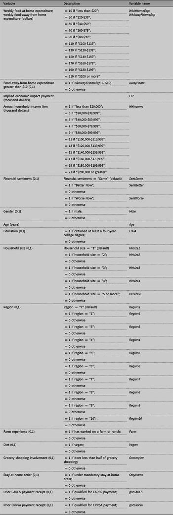


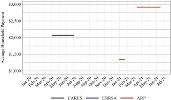
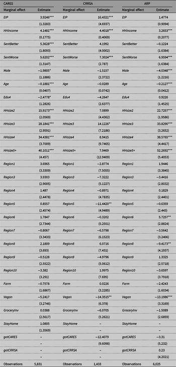


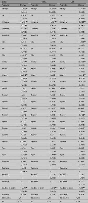
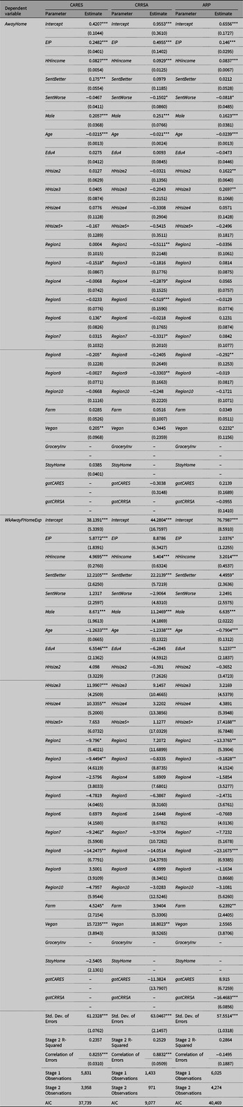
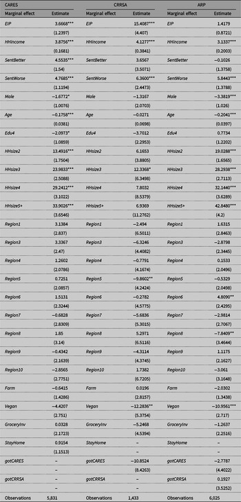


 Open access