


1. Introduction
Does child labor respond inversely to parental education? If so, whose education matters more, and for which forms of child labor? Curbing child labor in all forms remains an elusive undertaking, particularly in low- and middle-income settings. For the first time in nearly two decades, the global effort against child labor has stalled (ILO, 2021). Recent International [Labor] Organization (ILO) statistics indicate that 160 million children aged 5–17 were involved in child labor globally – up from 152 million in 2016 (ILO, 2017). This trend, however, masks significant heterogeneity in child labor prevalence at the sub-regional level. At present, child labor mitigation appears more challenging across many sub-Saharan African, South Asian, and Latin American countries (see Figure 1). Child labor is particularly pronounced in sub-Saharan Africa, where 1 in every 5 children aged 5–17 is a child laborer (ILO, 2017, 2021).

Figure 1. Regional prevalence of child labor.
At the same time, a key factor that potentially holds promise for child labor mitigation on the sub-continent is human capital acquisition. Studies on the cascading effects of parental education on child labor and schooling outcomes are well-documented in the development economics literature (Cigno et al., Reference Cigno, Rosati and Tzannatos2001; Das and Mukherjee, Reference Das and Mukherjee2007; Emerson and Souza, Reference Emerson and Souza2007; Kurosaki et al., Reference Kurosaki, Ito, Fuwa, Kubo and Sawada2006; Patrinos and Psacharapoulos, Reference Patrinos and Psacharopoulos1995; Rosati and Tzannatos, Reference Rosati and Tzannatos2006). While there exists overwhelming evidence suggesting a negative association between parental education and child labor, studies that aim to establish a causal link are rare. Potential confounders, such as cultural inclinations, prevailing local economic activity levels, inter alia, constitute common identification issues to contend with.
To overcome this identification challenge, I leverage demographic evidence on grandparents’ influence on grandchildren’s socioeconomic outcomes, highlighting the significance of familial living arrangements. For example, Zeng and Xie (Reference Zeng and Xie2014) noted that non-co-resident grandparents’ educational attainment has no bearing on grandchildren’s schooling outcomes conditional on parental characteristics. While earlier studies also provide support for this result (Erola and Moisio, Reference Erola and Moisio2007; Warren and Hauser, Reference Warren and Hauser1997), others find evidence that suggest otherwise (Chan and Boliver, Reference Chan and Boliver2013; Jæger, Reference Jæger2012). For instance, despite controlling for parents’ education, income, and wealth, Chan and Boliver (Reference Chan and Boliver2013) noted that grandparents exert a significant direct effect on their grandchildren’s occupational classes in Britain. This result, however, does not account for multigenerational co-residency (Chan and Boliver, Reference Chan and Boliver2013). Hence, conditioning on multigenerational co-residence, I use grandparents’ educational attainment as instruments to exploit plausibly exogenous variation in parents’ schooling.Footnote 1 Further, to explore the robustness of my results, I apply practical methods that relax the exclusion restriction assumption in an imperfect instruments framework (Conley et al., Reference Conley, Hansen and Rossi2012). In particular, I estimate bounds on the causal parameters of interest when the exclusion restriction assumptions are violated.
Using quasi-random access to education in Nyasaland (now Malawi) during the colonial period – mostly between 1859 and 1964, I present evidence on the effect of parental education on child labor outcomes, taking advantage of this opportune setting. First, the early stages of this period coincided with the peak of slave trade in Malawi, at the height of which men, women, and sometimes children were abducted in organized raids. With mostly firearms and sometimes ransom payments, the missionaries gradually brought these slave raiding forays under control. Upon rescue, the ex-slaves were enrolled in missionary schools as part of their rehabilitation (Allen, Reference Allen2008).
Second, even after missionary education became accessible to non-slave populations, many who sought to be educated were not admissible due to limited capacity (Allen, Reference Allen2008). Scarce qualified teaching personnel and inadequate school infrastructure prompted a form of rationing of missionary educational access. Hence, in my instrumental variable (IV) analysis, I use both grandparents’ education (reported as indicator variables for primary school completion) to instrument for a given parent’s level of education. Given that we are in the over-identified case (that is, there are more instruments than potentially endogenous variables), I am also able to check the credibility of my exclusion restriction assumptions.
The nexus between parental education and child labor deserves close research attention due to strong intergenerational persistence in child labor among low-income households (Aransiola and Justus, Reference Aransiola and Justus2018; Emerson and Souza, Reference Emerson and Souza2003). Educated parents typically demonstrate a proclivity for investing in their children’s education, which could rival alternative uses of the child’s time such as child labor work. Moreover, the productivity of the parents’ time as an input in the child’s education may increase with parental schooling (Andrabi et al., Reference Andrabi, Das and Khwaja2012; Behrman et al., Reference Behrman, Foster, Rosenweig and Vashishtha1999; Cigno et al., Reference Cigno, Rosati and Tzannatos2002). For instance, Andrabi et al. (Reference Andrabi, Das and Khwaja2012) observed that children with educated mothers spend more time on school-related activities at home, which competes with time spent working within and outside the home.
This paper focuses on another channel – parental engagement in nonfarm employment. Using a nationally representative survey data set on household demographics and child time use in Malawi, this study’s contributions to the broader child labor literature are threefold. First, it provides deeper insights into parental educational effects on child labor outcomes with a focus on nonfarm employment as a key mechanism. Second, by employing an instrumental variable (IV) strategy, this study attempts to address endogeneity issues inherent in the standard estimation of the relationships of interest. Moreover, this study considers child labor over a longer reference timeframe – an improvement upon earlier approaches, where a one-week recall period is routinely used. Third, it also accounts for child labor heterogeneity by considering two categories of child labor work: (1) household farm work, and (2) casual, part-time, or “ganyu” labor.Footnote 2
The IV estimation results indicate that there is a negative, and statistically significant relationship between parental education and “ganyu” labor participation. By contrast, I do not find a significant effect of maternal education on child farm work, while the father’s education is significantly negatively associated with both child labor measures. In other results, I find that maternal education significantly improves school attendance. On the other hand, I do not find a discernible impact of paternal education on schooling outcomes. These results are shown to be robust to some relaxation of the exclusion restriction assumptions. Using methods proposed by Acharya et al. (Reference Acharya, Blackwell and Sen2016), I also test whether nonfarm employment mediates the parental education effects on child time use. I find that nonfarm employment constitutes a more plausible mechanism for the maternal education effects on child labor.
The rest of the paper is organized as follows. Section 2 reviews related literature. Section 3 presents the data and some descriptive statistics. Section 4 illustrates the empirical strategy, and Section 5 addresses some endogeneity concerns. Section 6 summarizes the results. Section 7 presents a sensitivity analysis and Section 8 concludes.
2. Related literature
Parental education has the potential to mitigate child labor and improve school attendance (Bhalotra and Heady, Reference Bhalotra and Heady1998; Canagarajah and Coulombe, Reference Canagarajah and Coulombe1997; Canagarajah and Nielsen, Reference Canagarajah and Nielsen1999; Das and Mukherjee, Reference Das and Mukherjee2007; Emerson and Souza, Reference Emerson and Souza2007; Grootaert, Reference Grootaert1998; Hsin, Reference Hsin2007; Kurosaki et al., Reference Kurosaki, Ito, Fuwa, Kubo and Sawada2006; Tzannatos, Reference Tzannatos2003). While not considered a policy variable per se (Grootaert, Reference Grootaert1998), parental education – as a mitigation strategy – can be appealing as it is less intrusive compared to overt bans or prohibitions and has potentially longer-lasting effects (Cigno et al., Reference Cigno, Rosati and Tzannatos2002).
Besides altering parental preferences for/against child labor, education also affects parents’ occupational choices. These choices, in turn, have consequences for the next generation’s present and future labor market options. For example, Wantchekon et al. (Reference Wantchekon, Klašnja and Novta2015) documented in Benin that children with educated parents are significantly less likely to become farmers. Moreover, parents may also find it unfavorable to make their children work if the return to education to both parents and their children is sufficiently high. As such, most studies analyzing the correlates of child labor often examine both schooling and child work as these decisions are interlinked. While estimating a multi-stages sequential probit model, Grootaert (Reference Grootaert1998) noted that parental education improves the odds of exclusively attending school as well as combining school and work in Côte D’Ivoire. In Ghana, Canagarajah and Coulombe (Reference Canagarajah and Coulombe1997) discuss factors that jointly determine schooling and child labor decisions and found that school participation choices appear more responsive to parental education. I build on these early contributions to the literature, while focusing on parental education as the key variables of interest.
Also, relevant to this line of research is the extent to which the unitary household model – in lieu of the collective model – overlooks important intra-household power dynamics in the decision-making process (Browning et al., Reference Browning, Bourguignon, Chiappori and Lechene1994; Duflo, Reference Duflo2003; Thomas, Reference Thomas1990; Thomas, Reference Thomas1994). More importantly, the motivation for the collective model raises relevant questions about whose education matters most? This paper also contributes to a growing literature on the heterogeneous impacts of the mother’s and father’s education on child labor and schooling outcomes. In South Asia, Kurosaki et al. (Reference Kurosaki, Ito, Fuwa, Kubo and Sawada2006) find evidence, suggesting that the mother’s education is more important in reducing child labor in Andhra Pradesh. By contrast, Emerson and Souza (Reference Emerson and Souza2007) found that paternal education has a stronger negative influence on boys’ child labor status in Brazil. They also show that maternal schooling has a stronger positive impact on girls, while paternal education predicts higher attendance rates for boys.
Consistent with Das and Mukherjee (Reference Das and Mukherjee2007), Kurosaki et al. (Reference Kurosaki, Ito, Fuwa, Kubo and Sawada2006) also find that maternal education significantly reduces school dropout rates and child labor among boys in urban India. Patrinos and Psacharopoulos (Reference Patrinos and Psacharopoulos1995) also noted that maternal schooling has a strong and positive influence on children’s future employment prospects. Further, Bhalotra and Heady (Reference Bhalotra and Heady1998) review evidence of a negative and significant relationship between maternal schooling and household farm work among children in Pakistan and Ghana.
The prior literature has left additional gaps, which this study attempts to fill. One such underexplored gap concerns the heterogeneity of child labor and its implications for mitigation efforts. Some child labor activities are undoubtedly more harmful than others. As a consequence, we might expect such forms of child labor to decline dramatically with improvements in household socioeconomic conditions. Ali (Reference Ali2019) highlights the significance of accounting for child labor heterogeneity, demonstrating that only the worst forms of child work declined significantly with higher household income. The author posits that this could reflect parents’ non-pecuniary motivations for involving their children in non-hazardous forms of child work, such as unpaid family work. I extend my research scope to also address such heterogeneity by examining both household farm work and casual, part-time, or “ganyu” employment.
3. Data
Analysis for this study leverages data from the Malawian Integrated Household Survey (IHS) Program. The IHS is a product of collaborative work between the World Bank and the Malawian National Statistical Office as part of the LSMS - ISA (Living Standards Measurement Study - Integrated Surveys on Agriculture) household survey project. Extending across multiple rounds, the survey started off in 2010 with the implementation of the Third Integrated Household Survey (IHS3). The IHS3 sample was designed to be representative at the national-, regional-, and urban/rural levels. Following the IHS3, the 2013 Integrated Household Panel Survey (IHPS) was administered to follow-up on the 3,246 households initially interviewed in 2010. After tracking split-off individuals during follow-up, the final 2013 IHPS sample consisted of 4,000 households, linking back to 3,104 of the households interviewed during baseline.
The two most recent rounds of the panel survey: the Fourth (IHS4) and Fifth (IHS5) Integrated Household Surveys were conducted in 2016/17 and 2019/20, respectively. Due to funding challenges, the initial sampling frame was halved from 204 enumeration areas (EAs) during these latter rounds. The IHS4 ended with 2,508 households tracking an original target of 1,989 households in 102 EAs from the 2013 IHPS. Following a similar tracking guideline, the IHS5 grew to include 3,245 households, who were interviewed to collect detailed information on individual and household demographic variables, agricultural production, as well as community-level data. The data were collected through surveys conducted via interviews, with mostly the household head. For my analyses, I use the two latest IHPS waves (that is, the IHS4 and IHS5) for reasons I will specify shortly.
A major data limitation that often plagues many child labor studies is finding a suitable measure of child labor outcomes. In many developing country studies, a one-week reference period has been widely used to characterize child labor. However, such a short reference period may induce very little variation in child labor outcomes, which could be further exacerbated by measurement error, resulting in imprecise estimates (Dorman, Reference Dorman2008). As an example, the main child labor measures in the 2010 and 2013 IHPS include: (1) the number of hours in the last 7 days (before the survey) the child spent on agricultural activities, (2) the number of hours in the past week the child run or did any kind of nonagricultural work, and (3) the number of hours spent yesterday collecting water. Since interviewer visits occurred mostly between March and November, which overlaps with the peak season,Footnote 3 this might predict more child involvement in agricultural work relative to other child labor activities (e.g., nonfarm work).
Further, to the extent that the one-week reference period is too short to capture any meaningful variation in child labor activities, results may fail to fully reflect the true intensity of child labor work.Footnote 4 To partially obviate this risk, I use the two latest rounds of the IHPS. Unlike the earlier waves, the child labor measures reported in the IHS4 and IHS5 are over a relatively longer reference period (specifically, over the past 12 months), circumventing the aforementioned data limitations. Therefore, my two child labor measures include two indicator variables: one for whether the child contributed to household farming activities in the past year and another for whether (s)he engaged in any casual, part-time, or “ganyu” labor in the last 12 months.
For the child-level analysis, I restrict the sample to children aged 5–17, as that is the age range over which the ILO typically reports child labor statistics. Moreover, since a majority of children within this age bracket are of primary school-going age, this allows for studying any potential tradeoffs between school attendance and child labor. Summary statistics on both child- and household-level characteristics for the resulting sample are reported in Table 1. In the first column (the “All” column), I pool observations across both years and report descriptive statistics at both the child- and household-level in panels A and B, respectively.
Table 1. Summary statistics

Notes: Summary statistics are reported on households with children aged 5 – 17 with observations weighted using the 2016 panel sampling weights. Standard errors are reported in parentheses.
The average child in the sample is about 11 years old and there is an even split in gender representation. As panel A depicts, roughly half of all observation-years identify as female with females slightly overrepresented in the 2019 panel. A large fraction of children in the sample were reported to be currently attending school or did attend the just ended school session. It can also be inferred from the rather high attendance rate that few of these children can be considered full-time workers. Roughly 40% of the children in the sample contributed to any household farm work, and about 15% of them engaged in casual, part-time employment. Turning to panel B, women appear to receive less education relative to men.Footnote 5 This result is also reflected in the relatively lower educational attainment rates among both paternal and maternal grandmothers relative to grandfathers in the sample.
Table 2 presents evidence on child labor incidence and school attendance for the full sample by child gender and age. As expected, the child farm work incidence ratio is higher for boys (44%) compared to girls (39%). Also, older children (74%) are more likely to be involved in household farming activities relative to younger children (33%). This result seems intuitive given that older children are more likely to be out of school, signaling better availability to support household farm work. Moreover, farm work can be intense; hence, having a sturdier build, like boys and older children typically do, makes for better suitability for on-farm work. The data also reveal a gender disparity in casual, part-time, or “ganyu” employment. Boys are disproportionately more involved in this type of child labor work. The incidence ratio for casual, part-time employment is roughly 18% for boys, and 13% for girls. Again, the summary statistics indicate that older children have higher casual, part-time labor participation rates. Further, while a substantial proportion of children in the sample indicated that they do attend school, younger children have significantly better school attendance rates.
Table 2. Child labor incidence and school attendance by gender and age

Notes: Sample means are reported as percentages using the pooled sample across the 2016 and 2019 panel waves. The table also presents p-values for the null hypotheses that the differences in means by gender and age cohort are equal to zero.
Source: Author’s own calculations.
4. Empirical strategy
To quantify the effect of parental education on child labor participation, I first estimate the following linear effects model:
 $${y_{iht}} = \;{\alpha _0} + \boldsymbol{Edu{c_{ih}}\zeta} + \boldsymbol{x_{ht}\beta} \; + \;{\delta _d} + {\delta _t} + {\varepsilon _{iht}}$$
where y iht is an indicator variable, which takes the value 1 if child i in household h in time period t such that t ϵ {2016, 2019} was: (1) engaged in household farm work, (2) involved in any casual, part-time, or “ganyu” employment in the past 12 months, and zero otherwise; α 0 is a constant term; Educ ih is a vector denoting the mother’s and father’s years of schooling; ζ is a vector of parental education effects on child labor; x ht is a vector of time-varying controls including household size, a wealth index, number of male and female household members below age 6, total area of cultivated landholdings, and household distance to the nearest road. I also include controls for female-headship status, and religious affiliation; β is a vector of parameters on the time-varying household-level covariates to be estimated; δ d is a set of district fixed effects; δ t is a time dummy; and ε iht is an idiosyncratic error term with zero mean and standard deviation, σ ε . Standard errors are clustered at the child level to allow for correlation of errors for a child across years but not across children.
It is important to note that parental education will likely be predetermined by 2016 for a large fraction of children in the sample. Hence, the key explanatory variables of interest should not vary much over the survey years, if at all. That is, parental education is more or else a time-constant variable. As such, estimating the relationship between parental education and child labor using the traditional fixed effects approach will likely result in the estimated coefficients of interest getting dropped. This empirical challenge justifies the use of the pooled ordinary least squares (POLS) estimator. However, while the linear probability model (LPM) yields estimates that are easy to interpret, the estimated probabilities can sometimes lie outside the unit interval (that is, above one or below zero). Hence, as a robustness check, I also estimate equation (1) using a non-linear model.
5. Addressing endogeneity
The key explanatory variables of interest – that is, the mother’s and father’s education variables – may fail to satisfy the strict exogeneity assumption in the linear effects model. Reverse causality is unlikely to be an issue here as the data suggest that parental education generally precedes child labor decisions for most children in the sample. That said, correlation between parental education and confounders in the error term that also predict child labor participation will yet yield inconsistent estimates. For example, suppose that household agricultural productivity is an unmeasured omitted variable that is positively correlated with child labor (perhaps, due to missing or underdeveloped agricultural labor markets). In this setting, a positive correlation between parental education and productivity would attenuate any negative parental educational effect on child labor.
To address this endogeneity concern, I use an IV strategy. The IV method requires that we have an instrument or set of instruments that are strongly correlated with parental education (the relevancy condition), but affect child labor outcomes only through the key explanatory variable(s) of interest (the exclusion restriction). I use grandparents’ literacy as instruments for parental educational attainment.Footnote 6 In particular, the mother’s education is instrumented by each of her parents’ literacy rates, which are dichotomous variables taking the value 1 if they at least completed primary school and zero, otherwise.Footnote 7 Instrument selection was informed by the first generation’s (i.e., Malawian grandparents’) limited discretion in their choice of schooling outcomes, particularly during the colonial era. In the absence of a clear educational policy, combined with a lack of governmental support, Christian missionaries became the primary custodians of education pre-independence (McCracken, Reference McCracken2012). Upon rescue, these missions trained ex-slaves in schools, with some going on to become priests (McCracken, Reference McCracken2012). Further, even after missionary schools were open to non-slave populations, the financial toll on these missions meant that not all who sought missionary education could be admitted. Hence, the educational attainment of these children was almost quasi-random.
As I show later in the results section, it is rather straightforward to see how the chosen set of instruments satisfies the relevancy condition. However, what remains obscure is whether the necessary exclusion restriction assumptions are satisfied since these are not directly testable. That is, is it indeed the case that grandparents’ literacy is not correlated with other factors beyond the parents’ education that might also influence child labor participation? For example, an educated grandparent’s involvement in the child’s school work at home can potentially impact child labor decisions. This is because the grandparent could increase the returns to child school attendance by helping out with homework assignments, posing an identification challenge.
As a result of this potential violation of the exclusion restriction and other related concerns, I control for multigenerational co-residency in all my IV regressions. This strategy is motivated by findings in the demography literature, arguing that non-co-resident grandparents’ educational attainment exerts little to no influence on grandchildren’s schooling outcomes conditional of parental characteristics (Erola and Moisio, Reference Erola and Moisio2007; Warren and Hauser, Reference Warren and Hauser1997; Zeng and Xie, Reference Zeng and Xie2014). The multigenerational co-residence variables are binary indicators: one for whether the grandfather is dead or lives away from the child and another for whether the grandmother is deceased or resides away from the household. I include both variables in all my IV regressions, but in cases where these two variables are strongly correlated, I control for one or the other due to multicollinearity.
One could still argue that controlling for co-residency may not fully rule out all potential violations of the exclusion restriction. Grandparents could maintain other forms of interaction without physical proximity to their grandchildren. As such, it would have been ideal to conduct this analysis using only the sub-sample of children, who never met their grandparents. However, an initial exploration of the feasibility of such an analysis resulted in a nontrivial reduction in the effective sample size. Hence, the analysis proceeds with this limitation in mind. That said, I present results from a sensitivity analysis in Section 7, showing that my main findings are robust to explicitly allowing for some exclusion restriction violations.
Further, intrinsically linked to the missionaries’ educational curricula was the mandate to produce native purveyors of the Christian faith. As such, for the predominantly Islamic share of the population, self-selection out of missionary education will be common (Bone, Reference Bone1982). Hence, I also include religion dummies as additional controls. Nevertheless, as a robustness check, I also obtain 2SLS estimates while dropping parents who indicated being Muslim to investigate the stability of my results.Footnote 8
6. Results
6.1. Descriptive statistics
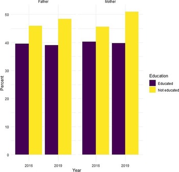
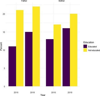
In Figures 2 and 3, I plot raw means for the two child labor outcomes against parental educational status for both survey years. A few important patterns emerge. First, Figure 2 shows that household farm labor participation is relatively common among children with uneducated parents. This pattern holds irrespective of the parent’s gender. Second, I find that household farm labor participation is relatively lower and remarkably stable over time among children with educated parents. By contrast, I observe an uptick in this outcome variable over time when parents are uneducated. Turning attention to Figure 3, I observe patterns that diverge somewhat from the trends in Figure 2. In relative terms, participation in this form of child labor work appears more pervasive among children with uneducated parents. However, the figure also shows that participation in casual, part-time, or “ganyu” employment increases over time for both sub-groups irrespective of parental educational status.

Figure 2. Child farm labor participation by parents’ educational status. Notes: Not educated implies zero years of education. Observations are weighted using 2016 panel weights.

Figure 3. Casual, part-time employment by parents’ educational status.
Notes: Not educated implies zero years of education. Observations are weighted using 2016 panel weights.
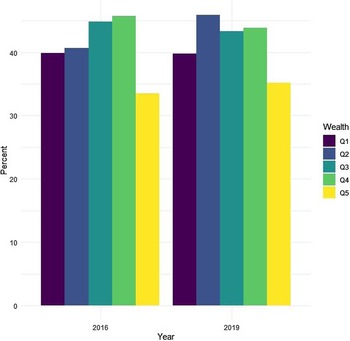
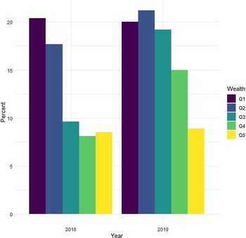
Figures 4 and 5 illustrate the relationship between child labor outcomes and household wealth graphically. While Figure 5 shows a consistently negative relationship between casual, part-time, or “ganyu” employment and household wealth, Figure 4 suggests a near non-linear trend. In particular, Figure 4 indicates that child farm work participation initially increases with household wealth, then begins to fall at extremely high levels of wealth. This finding is in line with Bhalotra and Heady (Reference Bhalotra and Heady1998)’s discovery that child labor use on household farms could worsen initially with wealth in the presence of multiple factor market failures.

Figure 4. Child farm labor participation by wealth quintiles.
Notes: Q1 denotes lowest wealth quintile. The wealth index is measured using household assets based on Principal Component Analysis. The wealth index variable was constructed using a principal component analysis where assets such as cars, motorcycles, bicycles, televisions, electric or gas stove, generators, washing machines, air conditioner, fan, radio, among others are given varying weights depending on the rarity of ownership among the sampled households. Observations are weighted using 2016 panel weights.

Figure 5. Casual, part-time employment by wealth quintiles. Notes: Q1 denotes lowest wealth quintile. The wealth index is measured using household assets based on Principal Component Analysis. The wealth index variable was constructed using a principal component analysis where assets such as cars, motorcycles, bicycles, televisions, electric or gas stove, generators, washing machines, air conditioner, fan, radio, among others are given varying weights depending on the rarity of ownership among the sampled households. Observations are weighted using 2016 panel weights.
6.2. OLS regression results
Linear probability model estimates for equation (1) are reported in the first two columns of Table 3. The columns present estimated coefficients of parental educational effects on child farm labor participation, and casual, part-time employment, respectively. Column (3) shows how school attendance responds to changes in parental education. Across all columns, I control for household-level covariates including the household size, a wealth index, number of male and female household members under age 6, household area of cultivated land, distance to the nearest road, religious affiliation of the household head, and female-headship status. A few results stand out.
Table 3. Estimates of parental education effects on child time use

Notes: Standard errors are reported in parentheses and are clustered at the child level. Control variables include household size, wealth index, size of household cultivated land, number of female household members under age 6, number of male household members under age 6, child’s gender, religion, female-headship status, and household distance to the nearest road. * p < 0.10, ** p < 0.05, *** p < 0.01.
The estimated coefficients for the mother’s educational attainment variable are negative and statistically significant for both child labor measures as reported in columns (1) and (2). In particular, an additional year of maternal schooling is associated with a 0.4 (0.6) percentage points decrease in the probability of child farm work participation (casual, part-time employment), on average. There is also a strong and negative association between paternal education and “ganyu” labor participation. Results in column (2) indicate that an additional year of paternal education decreases the child labor participation probability in “ganyu” by 0.9 percentage points, on average, ceteris paribus. By contrast, while the effect of the father’s education on child farm work is negative, it is not statistically different from zero. This result may indicate that child farm work participation could be viewed by fathers as a valuable source of work experience.
Table 3 also reports the effect of parental educational attainment on school attendance. Results are presented in column (3). Consistent with Kurosaki et al. (Reference Kurosaki, Ito, Fuwa, Kubo and Sawada2006), school attendance appears more responsive to maternal schooling. The point estimate of the coefficient on maternal education is 0.009, while the estimated coefficient for the father’s education is 0.003 – both estimated coefficients are statistically significant. In Table 4, I re-estimate equation (1) for both child labor outcomes and school attendance using a probit model. The estimated average partial effects of these probit models appear remarkably similar to the LPM estimates. Hence, in what follows, I prioritize the LPM estimates for ease of interpretation.
Table 5 reports the estimated effects of parental education on child labor outcomes and school attendance by the child’s gender. While girls appear less likely to engage in “ganyu” employment, I do not find any significant heterogeneous effects of parental education on child labor and school attendance by gender. That we do not find significant, heterogeneous parental educational effects on child time use perhaps suggests waning discrimination in human capital investments against girls.
Table 4. Average partial effects of parental education on child time use from probit model

Notes: Control variables include household size, wealth index, size of household cultivated land, number of female household members under age 6, number of male household members under age 6, child’s gender, religion, female-headship status, and household distance to the nearest road. Standard errors are reported in parentheses and are clustered at the child level. * p < 0.10, ** p < 0.05, *** p < 0.01.
Table 5. Effect of parental education on child time use by gender – LPM

Notes: Standard errors are reported in parentheses and are clustered at the child level. Control variables include household size, wealth index, size of household cultivated land, number of female household members under age 6, number of male household members under age 6, religion, female-headship status, and household distance to the nearest road. 1[Girl=1] is an indicator for whether the child is a female. * p < 0.10, ** p < 0.05, *** p < 0.01.
6.3. Mediation analysis
I now turn to the formal mediation analysis, which I conduct to assess whether parental nonfarm and wage employment are potential mechanisms through which parental education affects child time use. Higher educational attainment is typically associated with greater nonfarm labor force participation. To illustrate, uneducated households in the sample derive 21% of their monthly income from nonfarm employment, while households with any educated parent source close to half. Strong pull factors such as the relatively higher expected returns to nonfarm employment can induce a preference for nonfarm engagements among the educated. Hence, in identifying the effect of parental education on child labor outcomes, the role of the parents’ occupation cannot be ignored. For instance, Webbink et al. (Reference Webbink, Smits and de Jong2013) showed that children with fathers in nonfarm occupations were less involved in child labor. Indeed, parental sorting into nonfarm jobs can have two main effects on child labor. First, cash from nonfarm businesses and wage employment can buy labor and other labor-saving physical inputs, releasing the child from on-farm work. Second, if working on-farm requires close parental supervision, children with educated parents – who often prefer off-farm jobs – may be exempt from household farm work by design.
The mediation analysis setup is outlined next. I use the sequential g-estimation method proposed by Acharya et al. (Reference Acharya, Blackwell and Sen2016), by comparing the average treatment effect (ATE) of parental education on child time use with the average controlled direct effect (ACDE), which accounts for the effect of mediators.
Denote by y, the child time use outcome variable; T is the treatment variable of interest; X pre ( X post ) are pre- (post-) treatment covariates, where X pre includes indicators for the parents’ religious affiliation, female-headship status, and the child’s gender (see Bellemare et al. (Reference Bellemare, Lee and Novak2021) for a similar categorization); X post constitutes the household size, number of female household members below age 6, number of male household members under 6 years, a wealth index, and the total area of cultivated land in acres; M 1, M 2 are the mediators, which in our case are indicator variables for whether a parent was engaged in any nonfarm business and wage employment, respectively. The rest of the method proceeds as follows:
-
Regress y on the treatment (T), the covariates ( X pre , X post ) and the mediators (M 1, M 2):
(2) $${y_{iht}} = {\beta _0} + {\beta _1}{T_{ih}} + {\boldsymbol X}_{ht}^{pre}{{\boldsymbol\beta} ^{pre}} + {\boldsymbol X}_{ht}^{post}{{\boldsymbol \beta} ^{post}} + {\phi _1}{M_{1,ht}} + {\phi _2}{M_{2,ht}} + {\delta _d} + {\delta _t} + {\xi _{iht}}$$
-
Derive the de-mediated outcome variable as follows:
(3)
$${\tilde y_{iht}} = {y_{iht}} - {\boldsymbol X}_{ht}^{post}{\hat {\boldsymbol \beta} ^{post}} - {\hat \phi _1}{M_{1,ht}} - {\hat \phi _2}{M_{2,ht}}$$
-
Regress the de-mediated outcome variable on the treatment (T) and the pretreatment controls X pre :
(4)
$${\tilde y_{iht}} = {\lambda _0} + {\lambda _1}{T_{ih}} + {\boldsymbol X}_{ht}^{pre}{{\boldsymbol \lambda} ^{pre}} + {\delta _d} + {\delta _t} + {\upsilon _{iht}}$$


where the estimated parameter, ${\hat \lambda _1}$
denotes the ACDE of the treatment after the mediators have been accounted for. A failure to reject the null hypothesis, H
0:
${\hat \lambda _1}$
denotes the ACDE of the treatment after the mediators have been accounted for. A failure to reject the null hypothesis, H
0: ${\lambda _1}$
= 0 implies that the effect of the treatment T on y operates solely through the mediators, M
1, M
2 (Acharya et al., Reference Acharya, Blackwell and Sen2016; Bellemare et al., Reference Bellemare, Lee and Novak2021).
${\lambda _1}$
= 0 implies that the effect of the treatment T on y operates solely through the mediators, M
1, M
2 (Acharya et al., Reference Acharya, Blackwell and Sen2016; Bellemare et al., Reference Bellemare, Lee and Novak2021).
As a result of how the ACDEs are estimated, standard errors are bootstrapped with 500 replications. Results are summarized in Figure 6. I find that a large share (56%) of the maternal education effect on child farm labor participation can be explained by off-farm employment. I fail to reject the null that the direct effect after accounting for the mediators is zero at any of the traditional levels of significance. Similarly, I find that nonfarm employment mediates 35% of the “ganyu” employment-reducing effect of maternal education. However, the direct effect remains statistically significant at the 5% level. While I find that the mediators explain a nontrivial share (33%) of the paternal education effect on child farm labor participation, the OLS estimate is not statistically significant to begin with. Overall, these results suggest that nonfarm employment is a more likely mechanism through which maternal education affects child labor. That said, these results are only associational, hence, should be taken with some caution.

Figure 6. Mediation analysis - controlled direct effect of parental education on child time use. Notes: Coefficient estimate plots of average treatment effects (ATE) and the average controlled direct effects (ACDE) of parental education on child time use when both mediators (i.e., parental nonfarm and wage employment) are held fixed. Figure also presents the associated confidence intervals (CI) at the 90%, 95% and 99% levels, where the shortest CI width denotes the 90% CI, and so on. It also shows the share of the baseline OLS regression estimates that can be explained by both mediators.
6.4. 2SLS regression results
Next, I present results from the two-stage least squares (2SLS) estimator. I estimate separate models for the mother’s and father’s educational effects. First, I report estimates from the first stages of the IV analysis in Table 6. In column 1 (2), I report estimates from the regression of the mother’s (father’s) years of education on the maternal (paternal) grandparents’ literacy variables and other “exogenous” covariates for the full sample. Columns (3) through (6) show first-stage results disaggregated by child gender. I broadly find evidence of a strong correlation between parental educational attainment and grandparents’ literacy.
Table 6. First-stage regression results – LPM estimates

Notes: Standard errors are reported in parentheses and are clustered at the child level. * p < 0.10, ** p < 0.05, *** p < 0.01.
Table 7 reports the 2SLS estimation results. Columns (1)–(3) present the estimated coefficients for the two child labor measures and school attendance for the full sample in that order. The 2SLS estimates for the mother’s educational attainment variable are reported in panel A, while panel B presents the 2SLS estimates for the father’s educational effects. Following Olea and Pflueger (Reference Olea and Pflueger2013), I report the effective F statistic from a heteroskedastic, and cluster-robust test of the null of weak instruments across my IV specifications. A rejection of the null hypothesis signals a strong first stage. Further, I also report the Hansen J statistics with their corresponding p-values from the test of the null that the over-identifying restrictions are valid. Failure to reject the null in favor of the alternative hypothesis lends credence to the assumption that the necessary exclusion restrictions are satisfied.
Table 7. 2SLS estimates of the impact of parental education on child time use

Notes: Standard errors are reported in parentheses and are clustered at the child level. Other control variables include household size, wealth index, size of household cultivated land, number of female household members under age 6, number of male household members under age 6, religion, female-headship status, and household distance to the nearest road. * p < 0.10, ** p < 0.05, *** p < 0.01.
The weak IV tests reveal that the reported effective F statistics exceed the critical value for the τ = 30% weak instrument threshold across all specifications. That is, we can conclude that the instruments are strong. Second, the over-identification tests are reassuring as I roundly fail to reject the null hypothesis that the over-identifying restrictions are indeed valid. I now turn to the results.
First, I do not find a significant association between maternal education and child household farm work participation. That is, after instrumentation, the effect of the mother’s education on child farm work is attenuated (that is, it tends toward zero). By contrast, there is a strong negative association between maternal education and “ganyu” labor involvement. In particular, an additional year of maternal schooling is associated with a 1.5 percentage points decrease in the casual, part-time employment probability.
Second, I find a strong positive association between the mother’s education and school attendance. This result perhaps points to an improvement in the mother’s bargaining power, favoring more investments in “child goods”. Turning to panel B, the 2SLS estimates indicate a negative and statistically significant impact of paternal education on both child labor measures. Specifically, an additional year of paternal schooling is associated with a 2.6 (2.3) percentage points decline in the probability of child farm work (casual, part-time employment) participation, on average. On the other hand, the estimated coefficient for the school attendance outcome variable is not statistically different from zero. While unexpected, this result aligns with the hypothesis that fathers without education place a similar value on their children’s education as those who are educated. This may be tied to the significant subsidization of primary education in sub-Saharan Africa, making affordability at the primary school level less of an issue. Indeed, close to 90% of children, who work on household farms also attend school.
Table 8 presents 2SLS estimates of the impact of parental education on child time use by child gender. Panel A reports similar effects of maternal education on “ganyu” labor across gender. By contrast, I do not find a significant effect of maternal schooling on female school attendance, while the mother’s education strongly improves male school attendance. Similarly, the negative effect of paternal education on “ganyu” labor is only significant for the male sub-sample. Overall, these results suggest a bias in human capital investments in boys over girls, partly attributable to inheritance norms (Bhalotra and Heady, Reference Bhalotra and Heady2003).
Table 8. 2SLS estimates of the impact of parental education on child time use by gender

Notes: Standard errors are reported in parentheses and are clustered at the child level. Control variables include household size, wealth index, size of household cultivated land, number of female household members under age 6, number of male household members under age 6, religion, female-headship status, and household distance to the nearest road. * p < 0.10, ** p < 0.05, *** p < 0.01.
As a robustness check, I re-run my IV analysis, while restricting the sample to children born to non-Islamic parents. One might be concerned about selection of Islamic grandparents out of formal education due to Christian bias in the missionaries’ educational curricula. Results are reported in Table 9. The 2SLS estimates using this restricted sample are remarkably similar to my main results in Table 7. This suggests that potential selection of Islamic grandparents out of missionary education does not bias my main findings in any meaningful way.
Table 9. 2SLS estimates of the impact of parental education on child time use – robustness check

Notes: Standard errors are reported in parentheses and are clustered at the child level. Other control variables include household size, wealth index, size of household cultivated land, number of female household members under age 6, number of male household members under age 6, religion, female-headship status, and household distance to the nearest road. Note that the analysis is limited to non-Muslim households. * p < 0.10, ** p < 0.05, *** p < 0.01.
Next, I explore how child labor outcomes respond to parental educational attainment for children of differing age groups. To obtain these estimates, I interact the parental education variables with age dummies to estimate these heterogeneous effects. Results are presented in Figures 7 and 8 for the maternal education effects, while Figures 9 and 10 present the 2SLS estimates for the father’s education by child age. Some general patterns emerge. I do find some evidence of heterogeneous parental education effects by child age. In particular, I find that the estimated coefficients are statistically indistinguishable from zero for relatively younger children. By contrast, the estimated effects on older children’s child labor outcomes are negative and statistically significant, although less precisely estimated (that is, the confidence intervals are wider). This finding could be rationalized in part by the relatively lower child labor participation rates among younger children to begin with.

Figure 7. 2SLS estimates of the effect of maternal education on child farm work by age.

Figure 8. 2SLS estimates of the effect of maternal education on casual, part-time or “ganyu” labor employment by age.

Figure 9. 2SLS estimates of the effect of paternal education on child farm work by age.

Figure 10. 2SLS estimates of the effect of paternal education on casual, part-time or “ganyu” labor by age.
7. Imperfect instruments sensitivity analysis
In this sub-section, I examine the sensitivity of my IV results to a relaxation of the exclusion restriction. Following Conley et al. (Reference Conley, Hansen and Rossi2012), I obtain bounds on the causal effect of parental education, while allowing for a direct effect of grandparents’ literacy on child time use. While the over-identification tests suggest that the instruments may be valid, they are only necessary, but not sufficient conditions for instrument validity (Clarke and Matta, Reference Clarke and Matta2018).
Consider the IV model below:
 $${\boldsymbol Y} = \boldsymbol{X\beta} + \boldsymbol{Z\gamma} + \boldsymbol{\varepsilon} $$
 $${\boldsymbol X} = {\boldsymbol Z}{\bf{\Pi }} + {\boldsymbol V}$$
where
Y
is a vector of the child time use variables;
X
is a vector of the parental education variables;
Z
are the instruments (grandparents’ literacy); ${\bf \Pi\ }$
is a vector of first-stage coefficients;
${\bf \Pi\ }$
is a vector of first-stage coefficients; $\boldsymbol{\gamma}$
captures the direct effect of the instruments on the outcome variables. The exclusion restriction implies that
γ
= 0, indicating that the instruments affect child time use only through parental education.
$\boldsymbol{\gamma}$
captures the direct effect of the instruments on the outcome variables. The exclusion restriction implies that
γ
= 0, indicating that the instruments affect child time use only through parental education.
The imperfect instruments framework allows for relaxing the γ = 0 assumption. However, how do we choose a reasonable value for γ? One approach is to use Van Kippersluis and Rietveld (Reference Van Kippersluis and Rietveld2018)’s method, which leverages the zero first-stage test. This method involves finding a sub-sample for whom the first stage is zero by construction. However, if we estimate the first stage for this sub-group and it is non-zero, this indicates that the exclusion restriction is likely violated. We can then use the reduced form estimate of the effect of grandparents’ literacy on child time use as reasonable estimates for γ. Unfortunately, in our case, it is difficult to conceive of such a sub-sample for whom the first-stage is zero. Hence, I make some assumptions about the potential direction and magnitudes of the extent of the violation of the exclusion restriction, which I believe are still reasonable.
In particular, I assume that there is a direct negative association between grandparents’ literacy and child labor. In doing so, I set priors such that γ falls within the range [γ min , 0], where γ min ϵ {−0.001, −0.002, −0.003} to capture varying degrees of violation of the exclusion restriction.Footnote 9 Bounds are then obtained as the union of all confidence intervals for γ inside the assumed range [γ min , 0]. See Clarke and Matta (Reference Clarke and Matta2018) for details on the union of confidence intervals procedure. Results are presented in Tables 10 and 11 for the maternal and paternal education effects, respectively. The results indicate that the estimated bounds are relatively robust to worsening violations of the exclusion restriction.Footnote 10 Reassuringly, the 2SLS estimates fall within the estimated bounds, which do not include zero for the significant 2SLS results. Hence, despite substantial deviations from perfect exogeneity, my 2SLS results remain robust.Footnote 11
Table 10. 2SLS maternal educational impact - relaxing $\boldsymbol{\gamma}={\bf 0}$
assumption
$\boldsymbol{\gamma}={\bf 0}$
assumption

Notes: γ 1 and γ 2 represent the direct effect of the maternal grandparents’ literacy variables on child time use. Bounds derived using Conley et al. (Reference Conley, Hansen and Rossi2012)’s union of confidence intervals method. * p < 0.10, ** p < 0.05, *** p < 0.01.
Table 11. 2SLS paternal educational impact - relaxing $\boldsymbol{\gamma}={\bf 0}$
assumption
$\boldsymbol{\gamma}={\bf 0}$
assumption

Notes: γ 1 and γ 2 represent the direct effect of the paternal grandparents’ literacy variables on child time use. Bounds derived using Conley et al. (Reference Conley, Hansen and Rossi2012)’s union of confidence intervals method. * p < 0.10, ** p < 0.05, *** p < 0.01.
8. Conclusions
Child labor remains a pervasive phenomenon in sub-Saharan Africa. Given laws at both national and international levels to minimize child labor, the innocuous nature of household child labor participation makes it less noticeable and challenging to eradicate. In this paper, I revisit an important empirical question: does child labor respond inversely to parental education? There is a wide scope of anecdotal evidence suggesting that parental education reduces child labor participation; however, studies that attempt to address possible endogeneity issues as well as child labor work heterogeneity are rare. Moreover, very few studies have attempted to explore parental engagement in nonfarm employment as a potential mechanism driving these effects.
Using a nationally representative Malawian household survey data set, I find that parental education is generally child labor mitigating. There is a strong and negative effect of maternal schooling on “ganyu” labor involvement, but no effect on household farm work. In particular, an additional year of maternal (paternal) schooling is roughly associated with a 1.5 (2.3) percentage points decline in casual, part-time or “ganyu” employment, on average. Similarly, the return for an additional year of paternal schooling is a 2.6 percentage points decrease in child farm work. I find limited evidence of differing estimated effects by child gender for my LPM estimates; however, the estimated effects appear more pronounced for boys and older children for the 2SLS estimates. Results suggest that the impact of parental education on both child labor measures are mostly driven by older children, who are more likely to work on household farms at that age.
The study’s findings also indicate that child school attendance improves especially with higher maternal education. This finding is consistent with Das and Mukherjee (Reference Das and Mukherjee2007) and Kurosaki et al. (Reference Kurosaki, Ito, Fuwa, Kubo and Sawada2006), who also find strong and positive effects of maternal schooling on child school attendance. Nevertheless, the evidence of such effects on child school attendance is weak for the paternal education variable. Employing the imperfect instruments method proposed by Conley et al. (Reference Conley, Hansen and Rossi2012), I also show that my results are robust to varying violations of the exclusion restriction.
Finally, I also show that parental engagement in nonfarm employment pursuits could be an important mechanism underlying the negative effect of parental education on child labor outcomes. This is especially true for the maternal education effects on child farm work. Nonetheless, there are a few caveats to consider. Obviously, there could be other pathways through which the effect of parental education on child labor could be mediated. In addition, further analysis is required to uncover how parental engagement in the nonfarm economy directly impacts child time use. Is it earned nonfarm income or the transition to the nonfarm sector per se that predicts lower child labor participation? Supplementary qualitative data via interviews can provide additional insights.
Acknowledgments
My thanks to Ben Belton, my PhD Major Advisor, for valuable feedback on earlier versions of this paper. Also, I thank Thomas Reardon, Songqing Jin, and Trey Malone as well as Brown Bag seminar participants at Michigan State University for helpful comments. Finally, the suggestions of the two anonymous reviewers and editor Carlos Carpio, which markedly improved the paper, are much appreciated.
Data availability statement
Data are available upon request.
Author contributions
Conceptualization, E.A.; Methodology, E.A.; Formal Analysis, E.A.; Data Curation, E.A.; Writing – Original Draft, E.A., Writing – Review and Editing, E.A.; Supervision, E.A.; Funding Acquisition, E.A.
Financial support
Not applicable.
Competing interests
None.


 Open access