


1 Introduction
A bidispersive, or dual porosity, porous medium is one where the solid skeleton contains two types of pores. One type consists of the normal pores one recognizes, and these are the macropores. However, there are in addition micropores which may be cracks in the skeleton or may be deliberately created in a man made bidispersive material. For example, very small glass beads may be assembled to create an almost overall spherical ‘raspberry like’ shape, and these larger spheres then joined together form the bidispersive porous medium; see the picture given on page 3069 of Nield & Kuznetsov (Reference Nield and Kuznetsov2006a ). Hooman, Sauret & Dahari (Reference Hooman, Sauret and Dahari2015) describe a bidisperse porous medium consisting of thin plates and hot water pipes, while Imani & Hooman (Reference Imani and Hooman2017) deal with small blocks which are arranged into larger blocks, and other types of bidisperse porous media may be found in Straughan (Reference Straughan2015, p. 7, p. 184) and Straughan (Reference Straughan2017, pp. 2–8).
The porosity associated with the macropores is denoted by $\unicode[STIX]{x1D719}$
, i.e.
$\unicode[STIX]{x1D719}$
, i.e. $\unicode[STIX]{x1D719}$
is the ratio of the volume of the macropores to the total volume of the saturated porous material. The micropores are responsible for a porosity
$\unicode[STIX]{x1D719}$
is the ratio of the volume of the macropores to the total volume of the saturated porous material. The micropores are responsible for a porosity $\unicode[STIX]{x1D700}$
which is the ratio of the volume occupied by the micropores to the volume of the porous body which remains once the macropores are removed. This means the fraction of volume occupied by the micropores is
$\unicode[STIX]{x1D700}$
which is the ratio of the volume occupied by the micropores to the volume of the porous body which remains once the macropores are removed. This means the fraction of volume occupied by the micropores is $\unicode[STIX]{x1D700}(1-\unicode[STIX]{x1D719})$
whereas the fraction of the volume occupied by the solid skeleton is
$\unicode[STIX]{x1D700}(1-\unicode[STIX]{x1D719})$
whereas the fraction of the volume occupied by the solid skeleton is $(1-\unicode[STIX]{x1D700})(1-\unicode[STIX]{x1D719})$
.
$(1-\unicode[STIX]{x1D700})(1-\unicode[STIX]{x1D719})$
.
Dual-porosity porous media have been investigated in the chemical engineering and physics literature for some time. For example, Hashimoto & Smith (Reference Hashimoto and Smith1974), Kawazoe & Takeuchi (Reference Kawazoe and Takeuchi1975) and Taqvi, Vishnoi & Levan (Reference Taqvi, Vishnoi and Levan1997) concentrate on the adsorption of fluid on surfaces and diffusion in a bidisperse porous medium. Guyon, Oger & Plona (Reference Guyon, Oger and Plona1994) present an experimental study of sintered bimodal distributions of spheres with size ratio $1:4$
, and determine empirical relations for the effective resistivity of the pore fluid, and for the permeability of the materials, as a function of the porosity. Gerke & van Genuchten (Reference Gerke and van Genuchten1993a
) present parabolic equations for the pressures of fluid in the fracture (micro) and in the matrix (macro) together with parabolic equations for solute transport in both regions. Simulations of these equations are performed using finite elements. Gerke & van Genuchten (Reference Gerke and van Genuchten1993b
) perform similar modelling and analysis for a dual-porosity medium which is not fully saturated. Gerke & van Genuchten (Reference Gerke and van Genuchten1996) further the analysis of the above mentioned studies and use various geometrical shapes for the matrix geometries. Other references to the chemical engineering literature are provided in Chabanon, David & Goyeau (Reference Chabanon, David and Goyeau2015).
$1:4$
, and determine empirical relations for the effective resistivity of the pore fluid, and for the permeability of the materials, as a function of the porosity. Gerke & van Genuchten (Reference Gerke and van Genuchten1993a
) present parabolic equations for the pressures of fluid in the fracture (micro) and in the matrix (macro) together with parabolic equations for solute transport in both regions. Simulations of these equations are performed using finite elements. Gerke & van Genuchten (Reference Gerke and van Genuchten1993b
) perform similar modelling and analysis for a dual-porosity medium which is not fully saturated. Gerke & van Genuchten (Reference Gerke and van Genuchten1996) further the analysis of the above mentioned studies and use various geometrical shapes for the matrix geometries. Other references to the chemical engineering literature are provided in Chabanon, David & Goyeau (Reference Chabanon, David and Goyeau2015).
It would appear that temperature effects in bidisperse porous media were first investigated by Chen, Cheng & Zhao (Reference Chen, Cheng and Zhao2000b ) and Chen, Cheng & Hsu (Reference Chen, Cheng and Hsu2000a ). Chen et al. (Reference Chen, Cheng and Zhao2000b ) present results of an experimental study of channels packed with sintered copper bidispersed porous media. They showed that the bidisperse porous medium is a highly effective two-phase heat sink. Chen et al. (Reference Chen, Cheng and Hsu2000a ) present measurements of two samples of bidisperse porous media saturated with three different fluids. They find that the effective thermal conductivity of a bidisperse porous medium is smaller than that of the equivalent monodispersed porous medium.
Specific theoretical approaches of fluid flow in isothermal dual-porosity media appear to have begun with Vernescu (Reference Vernescu1990) who employed Stokes flow in the fluid and Darcy theory for flow in porous blocks immersed (and held fixed) in the fluid. He identified three regimes where the overall flow could be described by Darcy theory, Brinkman theory or by Stokes flow, depending on the characteristic length of the porous obstacles and the distance between these. Moutsopoulos & Koch (Reference Moutsopoulos and Koch1999) developed a model for flow in a bidisperse porous medium by assuming the smaller grains only affect the flow through their permeability $K_{2}$
. They use a Brinkman theory to model flow in a bidisperse porous medium with one velocity field. Their equations governing incompressible flow in a bidisperse porous medium have the form
$K_{2}$
. They use a Brinkman theory to model flow in a bidisperse porous medium with one velocity field. Their equations governing incompressible flow in a bidisperse porous medium have the form
 $$\begin{eqnarray}-\unicode[STIX]{x1D707}\unicode[STIX]{x0394}u_{i}+p_{,i}+{\displaystyle \frac{\unicode[STIX]{x1D707}}{K_{2}}}\,u_{i}=0,\quad u_{i,i}=0,\end{eqnarray}$$
where $\unicode[STIX]{x1D707}$
is the fluid viscosity,
$\unicode[STIX]{x1D707}$
is the fluid viscosity, $p$
pressure and
$p$
pressure and $u_{i}$
the velocity in the porous medium. The study of Moutsopoulos & Koch (Reference Moutsopoulos and Koch1999) concentrates on being able to follow diffused material in the porous medium and to this end they couple equations (1.1) with an equation for the tracer concentration,
$u_{i}$
the velocity in the porous medium. The study of Moutsopoulos & Koch (Reference Moutsopoulos and Koch1999) concentrates on being able to follow diffused material in the porous medium and to this end they couple equations (1.1) with an equation for the tracer concentration, $c$
,
$c$
,
 $$\begin{eqnarray}{\displaystyle \frac{\unicode[STIX]{x2202}c}{\unicode[STIX]{x2202}t}}+(v_{i}c)_{,i}=D\unicode[STIX]{x0394}c,\end{eqnarray}$$
where $v_{i}=u_{i}/(1-\unicode[STIX]{x1D719}_{2})$
,
$v_{i}=u_{i}/(1-\unicode[STIX]{x1D719}_{2})$
, $\unicode[STIX]{x1D719}_{2}$
being the volume fraction of the smaller particles, and
$\unicode[STIX]{x1D719}_{2}$
being the volume fraction of the smaller particles, and $D$
is the diffusion coefficient. Throughout we employ standard indicial notation in conjunction with the Einstein summation convention. Thus, a repeated index sums from 1 to 3 whereas a free index may take the values 1, 2 or 3. For example,
$D$
is the diffusion coefficient. Throughout we employ standard indicial notation in conjunction with the Einstein summation convention. Thus, a repeated index sums from 1 to 3 whereas a free index may take the values 1, 2 or 3. For example,
 $$\begin{eqnarray}u_{i,i}\equiv \mathop{\sum }_{i=1}^{3}{\displaystyle \frac{\unicode[STIX]{x2202}u_{i}}{\unicode[STIX]{x2202}x_{i}}}={\displaystyle \frac{\unicode[STIX]{x2202}u_{1}}{\unicode[STIX]{x2202}x}}+{\displaystyle \frac{\unicode[STIX]{x2202}u_{2}}{\unicode[STIX]{x2202}y}}+{\displaystyle \frac{\unicode[STIX]{x2202}u_{3}}{\unicode[STIX]{x2202}z}};\end{eqnarray}$$
or
 $$\begin{eqnarray}\unicode[STIX]{x1D706}_{ij}u_{j}\equiv \mathop{\sum }_{j=1}^{3}\unicode[STIX]{x1D706}_{ij}u_{j}=\unicode[STIX]{x1D706}_{i1}u_{1}+\unicode[STIX]{x1D706}_{i2}u_{2}+\unicode[STIX]{x1D706}_{i3}u_{3},\quad i=1,2\text{ or }3;\end{eqnarray}$$
for some tensor $\unicode[STIX]{x1D706}_{ij}$
, or
$\unicode[STIX]{x1D706}_{ij}$
, or
 $$\begin{eqnarray}(v_{i}c)_{,i}\equiv \mathop{\sum }_{i=1}^{3}{\displaystyle \frac{\unicode[STIX]{x2202}}{\unicode[STIX]{x2202}x_{i}}}\,(v_{i}c)={\displaystyle \frac{\unicode[STIX]{x2202}}{\unicode[STIX]{x2202}x}}(cv_{1})+{\displaystyle \frac{\unicode[STIX]{x2202}}{\unicode[STIX]{x2202}y}}(cv_{2})+{\displaystyle \frac{\unicode[STIX]{x2202}}{\unicode[STIX]{x2202}z}}(cv_{3}).\end{eqnarray}$$
A key development in the theory of bidisperse porous media is due to Nield & Kuznetsov (Reference Nield and Kuznetsov2005) who develop and utilize a novel model which employs different velocities $U_{i}^{f}$
and
$U_{i}^{f}$
and $U_{i}^{p}$
in the macro and micropores, different pressures
$U_{i}^{p}$
in the macro and micropores, different pressures $p^{f}$
and
$p^{f}$
and $p^{p}$
and additionally different temperatures
$p^{p}$
and additionally different temperatures $T^{f}$
and
$T^{f}$
and $T^{p}.$
Throughout we use
$T^{p}.$
Throughout we use $f$
to denote macro and
$f$
to denote macro and $p$
to denote microquantities. This model was explicitly adapted to thermal convection in Nield & Kuznetsov (Reference Nield and Kuznetsov2006a
), where they used Brinkman theory for both the macro and microphases and presented a linear instability analysis. A global nonlinear energy stability analysis for the same problem was given by Straughan (Reference Straughan2009), who derived nonlinear stability Rayleigh numbers which were lower than the linear instability ones of Nield & Kuznetsov (Reference Nield and Kuznetsov2006a
). Straughan (Reference Straughan2015, pp. 183–202) developed both linear instability and global nonlinear stability analyses for thermal convection in a Nield–Kuznetsov bidisperse porous medium when Darcy theory was employed in both the macro and microphases. In that work there is a large gap between the critical Rayleigh numbers of linear theory and those for the nonlinear threshold. While this does not imply the existence of sub-critical instabilities, it does leave open the possibility. Also, exchange of stabilities has not been proved in either the Brinkman–Brinkman or Darcy–Darcy case when there are two temperatures and so there is a possibility of oscillatory convection in addition to the already observed stationary convection.
$p$
to denote microquantities. This model was explicitly adapted to thermal convection in Nield & Kuznetsov (Reference Nield and Kuznetsov2006a
), where they used Brinkman theory for both the macro and microphases and presented a linear instability analysis. A global nonlinear energy stability analysis for the same problem was given by Straughan (Reference Straughan2009), who derived nonlinear stability Rayleigh numbers which were lower than the linear instability ones of Nield & Kuznetsov (Reference Nield and Kuznetsov2006a
). Straughan (Reference Straughan2015, pp. 183–202) developed both linear instability and global nonlinear stability analyses for thermal convection in a Nield–Kuznetsov bidisperse porous medium when Darcy theory was employed in both the macro and microphases. In that work there is a large gap between the critical Rayleigh numbers of linear theory and those for the nonlinear threshold. While this does not imply the existence of sub-critical instabilities, it does leave open the possibility. Also, exchange of stabilities has not been proved in either the Brinkman–Brinkman or Darcy–Darcy case when there are two temperatures and so there is a possibility of oscillatory convection in addition to the already observed stationary convection.
The two velocity theory of Nield & Kuznetsov (Reference Nield and Kuznetsov2005, Reference Nield and Kuznetsov2006a ) has been successfully applied to many problems of forced convection, numerical simulation and other flows by Nield & Kuznetsov (Reference Nield and Kuznetsov2004, Reference Nield and Kuznetsov2006b , Reference Nield and Kuznetsov2007, Reference Nield and Kuznetsov2008, Reference Nield and Kuznetsov2011, Reference Nield and Kuznetsov2013), Rees, Nield & Kuznetsov (Reference Rees, Nield and Kuznetsov2008b ), Kumari & Pop (Reference Kumari and Pop2009), Revnic et al. (Reference Revnic, Grosan, Pop and Ingham2009), Narasimhan & Reddy (Reference Narasimhan and Reddy2011a ,Reference Narasimhan and Reddy b ), Narasimhan, Reddy & Dutta (Reference Narasimhan, Reddy and Dutta2012), Magyari (Reference Magyari2013), Nield & Bejan (Reference Nield and Bejan2013), Nield (Reference Nield2016), Wang et al. (Reference Wang, Vafai, Li and Cen2017), Wang & Li (Reference Wang and Li2018) and Patrulescu, Grosan & Pop (Reference Patrulescu, Grosan and Pop2020).
Two very important articles pertaining to the theory of Nield & Kuznetsov (Reference Nield and Kuznetsov2006a
) are those of Hooman et al. (Reference Hooman, Sauret and Dahari2015), and Imani & Hooman (Reference Imani and Hooman2017). The work of Hooman et al. (Reference Hooman, Sauret and Dahari2015) analyses heat transfer in a plate–fin heat exchanger and they perform the first calculation of values for the momentum transfer coefficient for flow between the macro and microphases. This is a key parameter in the Nield & Kuznetsov (Reference Nield and Kuznetsov2006a
) theory and previously no values were known. The work of Imani & Hooman (Reference Imani and Hooman2017) uses a bidisperse porous medium consisting of blocks of porous material which are themselves composed of smaller microblocks. They note that the theory of Nield & Kuznetsov (Reference Nield and Kuznetsov2006a
) involves two unknown parameters, namely the heat transfer coefficient and the interfacial momentum transfer coefficient, and they also point out that the theory relies on the assumption of local thermal equilibrium within the microporous medium. The heat transfer coefficient issue is addressed by Rees (Reference Rees2009, Reference Rees2010), and the interfacial momentum concern was addressed by Hooman et al. (Reference Hooman, Sauret and Dahari2015), as stated above. However, the local thermal issue is resolved in Imani & Hooman (Reference Imani and Hooman2017). They show that when the macropores are relatively large compared to the micropores then one may assume the temperatures of the solid skeleton match those of the fluid in the macro and microphases, i.e. there is local thermal equilibrium. Precisely, they write $\ldots$
‘it is shown that departure from the local thermal equilibrium condition is observed for the higher values of the Rayleigh number, microporous porosity, solid–fluid thermal conductivity ratio, and the smaller values of the macropores volume fraction’.
$\ldots$
‘it is shown that departure from the local thermal equilibrium condition is observed for the higher values of the Rayleigh number, microporous porosity, solid–fluid thermal conductivity ratio, and the smaller values of the macropores volume fraction’.
When large temperature differences are expected in the macro and micropores the two temperature theory should be used, for example when hot fluid is injected into a cold skeleton, see Rees, Bassom & Siddheshwar (Reference Rees, Bassom and Siddheshwar2008a
), Rees & Bassom (Reference Rees and Bassom2010). However, for many applications a single temperature, $T$
, may suffice. With this in mind Falsaperla, Mulone & Straughan (Reference Falsaperla, Mulone and Straughan2016) and Gentile & Straughan (Reference Gentile and Straughan2017a
) adapted the Nield & Kuznetsov (Reference Nield and Kuznetsov2006a
) theory to a single temperature. This reduced theory has subsequently been successfully employed in a variety of contexts by Capone, De Luca & Gentile (Reference Capone, De Luca and Gentile2020), Gentile & Straughan (Reference Gentile and Straughan2017b
) and Straughan (Reference Straughan2018, Reference Straughan2019a
,Reference Straughan
b
). All of the just cited articles employing a single temperature assume the flow in both the macro and microphases is described by Darcy theory.
$T$
, may suffice. With this in mind Falsaperla, Mulone & Straughan (Reference Falsaperla, Mulone and Straughan2016) and Gentile & Straughan (Reference Gentile and Straughan2017a
) adapted the Nield & Kuznetsov (Reference Nield and Kuznetsov2006a
) theory to a single temperature. This reduced theory has subsequently been successfully employed in a variety of contexts by Capone, De Luca & Gentile (Reference Capone, De Luca and Gentile2020), Gentile & Straughan (Reference Gentile and Straughan2017b
) and Straughan (Reference Straughan2018, Reference Straughan2019a
,Reference Straughan
b
). All of the just cited articles employing a single temperature assume the flow in both the macro and microphases is described by Darcy theory.
The configuration of blocks which are themselves smaller blocks of solid allow Imani & Hooman (Reference Imani and Hooman2017) to employ Navier–Stokes theory in the fluid with a regular heat equation in the solid skeleton. They use lattice-Boltzmann theory to justify the local thermal equilibrium (LTE) theory of Nield & Kuznetsov (Reference Nield and Kuznetsov2006a ). This gives reason for us to employ LTE theory throughout the bidisperse porous medium. From the mathematical point of view, using LTE theory, i.e. a single temperature, modifies the problem so we are able to show that exchange of stabilities holds, and we also show that the linear instability threshold is the same as the global nonlinear one. Thus, linear instability theory correctly captures the onset of thermal convection. We have not been able to prove such a result when two temperatures are present.
In this paper we allow for the possibility of larger pores where we employ a Brinkman theory, while still retaining Darcy theory in the micropores. We believe this is the first time a mixed Darcy–Brinkman model has been employed in bidispersive flow. It is worth noting that the original model of Nield & Kuznetsov (Reference Nield and Kuznetsov2006a ) employed a Brinkman theory in both the macro and micropores. Thermal convection in the two temperature bidispersive theory with Brinkman effects in both the macro and microphases, or with Darcy effects in both phases, is discussed at length in chapter 13 of Straughan (Reference Straughan2015).
It is very important to realize that the Brinkman theory, even in a single-porosity medium, will yield very different stability bounds to those found with Darcy theory, see the detailed analysis of Rees (Reference Rees2002). Furthermore, Straughan (Reference Straughan2016) has shown that Darcy theory may lead to oscillatory convection in a resonance problem whereas the equivalent Brinkman problem yields stationary convection. Hence, Darcy and Brinkman theory can lead to different physical effects.
We believe the use of Brinkman theory for the macrophase is justified since we are envisaging a material with relatively large macropores, i.e. a relatively large macroporosity. Givler & Altobelli (Reference Givler and Altobelli1994) justify use of Brinkman theory when the porous medium is an open cell rigid foam, porosity $\unicode[STIX]{x1D719}=0.972$
and Durlofsky & Brady (Reference Durlofsky and Brady1987) achieve a similar justification for
$\unicode[STIX]{x1D719}=0.972$
and Durlofsky & Brady (Reference Durlofsky and Brady1987) achieve a similar justification for $\unicode[STIX]{x1D719}\geqslant 0.95$
. Rubinstein (Reference Rubinstein1986a
) establishes a similar justification when
$\unicode[STIX]{x1D719}\geqslant 0.95$
. Rubinstein (Reference Rubinstein1986a
) establishes a similar justification when $\unicode[STIX]{x1D719}\geqslant 0.8$
; Rubinstein (Reference Rubinstein1986b
) proves a beautiful result whereby he gives a rigorous proof of the convergence of Stokes’ equation in domains containing a random distribution of identical spheres to Brinkman’s equation. The Brinkman equation in bidisperse porous media is employed by Moutsopoulos & Koch (Reference Moutsopoulos and Koch1999). Chabanon et al. (Reference Chabanon, David and Goyeau2015) to define three scales for a bidisperse porous material, a macroscopic scale, a microscopic scale and also a mesoscopic scale. They use averaging techniques in the mesoscopic scale and show the relevant equation is one of Brinkman form where the Navier–Stokes Laplacian term and the Darcy linear term are simultaneously present. They present numerical results for a bidisperse material which is composed of staggered cylinders at both macroscopic and microscopic scales with a porosity of 0.6, which is in the same range as that noted by Nield (Reference Nield2000, p. 168).
$\unicode[STIX]{x1D719}\geqslant 0.8$
; Rubinstein (Reference Rubinstein1986b
) proves a beautiful result whereby he gives a rigorous proof of the convergence of Stokes’ equation in domains containing a random distribution of identical spheres to Brinkman’s equation. The Brinkman equation in bidisperse porous media is employed by Moutsopoulos & Koch (Reference Moutsopoulos and Koch1999). Chabanon et al. (Reference Chabanon, David and Goyeau2015) to define three scales for a bidisperse porous material, a macroscopic scale, a microscopic scale and also a mesoscopic scale. They use averaging techniques in the mesoscopic scale and show the relevant equation is one of Brinkman form where the Navier–Stokes Laplacian term and the Darcy linear term are simultaneously present. They present numerical results for a bidisperse material which is composed of staggered cylinders at both macroscopic and microscopic scales with a porosity of 0.6, which is in the same range as that noted by Nield (Reference Nield2000, p. 168).
Bidisperse porous media are being increasingly employed in industry or are being recognized as being key to many real life processes and so we believe understanding a macro-Brinkman–micro-Darcy model is essential. The application areas for double-porosity media (bidispersive) are very varied and include for example, chemical engineering technology, see e.g. Enterria et al. (Reference Enterria, Suarez-Garcia, Martinez-Alonso and Tascon2014); coal stockpiling, see Hooman & Maas (Reference Hooman and Maas2014); gas shale storage, see Alnoaimi & Kovscek (Reference Alnoaimi and Kovscek2019); heat pipe technology, see Lin et al. (Reference Lin, Liu, Huang and Chen2011) and Mottet & Prat (Reference Mottet and Prat2016); hydraulic fracturing of subterranean rocks for natural gas, see e.g. Jiang et al. (Reference Jiang, Wang, Bian, Li, Liu, Wu and Zhou2018), Kim & Moridis (Reference Kim and Moridis2015) and Zhang et al. (Reference Zhang, Li, Zou, Li, Xie and Wang2019); understanding landslides, see e.g. Borja, Liu & White (Reference Borja, Liu and White2012) and Montrasio, Valentino & Losi (Reference Montrasio, Valentino and Losi2011); and in particular with reference to the caldera in the Campi Flegrei in the area to the west of Naples, see Scotto di Santolo & Evangelista (Reference Scotto di Santolo, Evangelista, Chen, Zhang, Ho, Wu and Li2008).
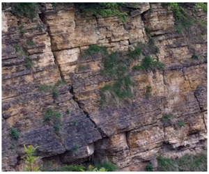
It is important to include temperature effects in bidispersive flow because thermal stresses are likely to induce cracking in the solid skeleton and this produces micropores, cf. Homand-Etienne & Houpert (Reference Homand-Etienne and Houpert1989), Gelet, Loret & Khalili (Reference Gelet, Loret and Khalili2012) and Kim & Hosseini (Reference Kim and Hosseini2015).
In this work we derive a model for thermal convection in a bidisperse porous medium with one temperature field allowing for Brinkman effects in the macropores whilst retaining only Darcy effects in the micropores. Thermal convection is analysed in a horizontal porous layer and we prove the strong result that the linear instability threshold is exactly the same as the global nonlinear stability boundary obtained from energy stability theory. This result is proved for anisotropic macro and micropermeabilities although we restrict our attention to the physically important case of symmetric permeability tensors. In addition, we allow for general thermal boundary conditions encompassing the case of radiation and a prescribed temperature. We also include a detailed account of numerical results in the prescribed temperature case when the permeabilities are isotropic.
Table 1. List of nomenclature.

2 Governing equations in the isotropic case
A general theory for bidisperse porous media is presented in Franchi, Nibbi & Straughan (Reference Franchi, Nibbi and Straughan2017). These writers combine the model of Nield & Kuznetsov (Reference Nield and Kuznetsov2006a ) for a bidisperse porous medium together with the local thermal non-equilibrium equations for a monodisperse porous material of Nield (Reference Nield1998) and Banu & Rees (Reference Banu and Rees2002), to derive a theory which involves macro and micropore averaged velocities, an individual solid skeleton, macro and micro temperature fields. This may be seen as follows.
For an isotropic bidisperse porous medium the momentum and continuity equations of Nield & Kuznetsov (Reference Nield and Kuznetsov2006a ) may be written
 $$\begin{eqnarray}\left.\begin{array}{@{}ll@{}} & \displaystyle -{\displaystyle \frac{\unicode[STIX]{x1D707}}{K_{f}}}\,U_{i}^{f}+\tilde{\unicode[STIX]{x1D707}}\unicode[STIX]{x0394}U_{i}^{f}-\unicode[STIX]{x1D701}(U_{i}^{f}-U_{i}^{p})-p_{,i}^{f}\\[5.0pt] & \displaystyle \quad +\unicode[STIX]{x1D70C}_{F}g\unicode[STIX]{x1D6FC}k_{i}\left[{\displaystyle \frac{\unicode[STIX]{x1D719}}{\unicode[STIX]{x1D719}+\unicode[STIX]{x1D700}(1-\unicode[STIX]{x1D719})}}\,T^{f}+{\displaystyle \frac{\unicode[STIX]{x1D700}(1-\unicode[STIX]{x1D719})}{\unicode[STIX]{x1D719}+\unicode[STIX]{x1D700}(1-\unicode[STIX]{x1D719})}}\,T^{p}\right]=0,\\[5.0pt] & \displaystyle U_{i,i}^{f}=0,\\[5.0pt] & \displaystyle -{\displaystyle \frac{\unicode[STIX]{x1D707}}{K_{p}}}\,U_{i}^{p}-\unicode[STIX]{x1D701}(U_{i}^{p}-U_{i}^{f})-p_{,i}^{p}\\[5.0pt] & \displaystyle \quad +\unicode[STIX]{x1D70C}_{F}g\unicode[STIX]{x1D6FC}k_{i}\left[{\displaystyle \frac{\unicode[STIX]{x1D719}}{\unicode[STIX]{x1D719}+\unicode[STIX]{x1D700}(1-\unicode[STIX]{x1D719})}}\,T^{f}+{\displaystyle \frac{\unicode[STIX]{x1D700}(1-\unicode[STIX]{x1D719})}{\unicode[STIX]{x1D719}+\unicode[STIX]{x1D700}(1-\unicode[STIX]{x1D719})}}\,T^{p}\right]=0,\\[5.0pt] & U_{i,i}^{p}=0,\end{array}\right\}\end{eqnarray}$$
where $k_{i}=\unicode[STIX]{x1D6FF}_{i3}$
and where the divergence free conditions (continuity equations) express the fact that the fluid is incompressible. Nield & Kuznetsov (Reference Nield and Kuznetsov2006a
) additionally include a Laplacian (Brinkman) term in equation (2.1)
$k_{i}=\unicode[STIX]{x1D6FF}_{i3}$
and where the divergence free conditions (continuity equations) express the fact that the fluid is incompressible. Nield & Kuznetsov (Reference Nield and Kuznetsov2006a
) additionally include a Laplacian (Brinkman) term in equation (2.1) $_{3}$
but we only use Darcy theory in the microphase. In these equations
$_{3}$
but we only use Darcy theory in the microphase. In these equations $U_{i}^{f},U_{i}^{p}$
,
$U_{i}^{f},U_{i}^{p}$
, $p^{f},p^{p}$
,
$p^{f},p^{p}$
, $T^{f}$
and
$T^{f}$
and $T^{p}$
are the pore averaged velocities, pressure and temperature fields in the macro (f) phase and micro (p) phase, respectively. The quantities
$T^{p}$
are the pore averaged velocities, pressure and temperature fields in the macro (f) phase and micro (p) phase, respectively. The quantities $\unicode[STIX]{x1D707},\tilde{\unicode[STIX]{x1D707}},\unicode[STIX]{x1D70C},K_{f}$
and
$\unicode[STIX]{x1D707},\tilde{\unicode[STIX]{x1D707}},\unicode[STIX]{x1D70C},K_{f}$
and $K_{p}$
denote the dynamic viscosity of the fluid, the Brinkman viscosity, the fluid density, the macropermeability and the micropermeability. In addition,
$K_{p}$
denote the dynamic viscosity of the fluid, the Brinkman viscosity, the fluid density, the macropermeability and the micropermeability. In addition, $g,\unicode[STIX]{x1D6FC}$
and
$g,\unicode[STIX]{x1D6FC}$
and $\unicode[STIX]{x1D70C}_{F}$
denote gravity, thermal expansion coefficient of the fluid and a constant reference density, since in the buoyancy terms a Boussinesq approximation is employed to write the fluid density as a linear function of
$\unicode[STIX]{x1D70C}_{F}$
denote gravity, thermal expansion coefficient of the fluid and a constant reference density, since in the buoyancy terms a Boussinesq approximation is employed to write the fluid density as a linear function of $T^{f}$
and
$T^{f}$
and $T^{p}$
. Finally,
$T^{p}$
. Finally, $\unicode[STIX]{x1D701}$
is a coefficient which represents the momentum transfer between the macro and microphases. All the variables and parameters defined above are listed in table 1.
$\unicode[STIX]{x1D701}$
is a coefficient which represents the momentum transfer between the macro and microphases. All the variables and parameters defined above are listed in table 1.
In the solid skeleton, the macrophase and in the microphase the energy balances may be separately written to account for interactions between the temperatures of each phase. Taking into account the volume fraction occupied by each phase the energy balances are written as
 $$\begin{eqnarray}\left.\begin{array}{@{}c@{}}\displaystyle \unicode[STIX]{x1D716}_{1}(\unicode[STIX]{x1D70C}c)_{s}T_{,t}^{s}=\unicode[STIX]{x1D716}_{1}\unicode[STIX]{x1D705}_{s}\unicode[STIX]{x0394}T^{s}+s_{1}(T^{f}-T^{s})+s_{2}(T^{p}-T^{s}),\\[5.0pt] \displaystyle \unicode[STIX]{x1D719}(\unicode[STIX]{x1D70C}c)_{f}T_{,t}^{f}+\unicode[STIX]{x1D719}(\unicode[STIX]{x1D70C}c)_{f}V_{i}^{f}T_{,i}^{f}=\unicode[STIX]{x1D719}\unicode[STIX]{x1D705}_{f}\unicode[STIX]{x0394}T^{f}+h(T^{p}-T^{f})+s_{1}(T^{s}-T^{f}),\\[5.0pt] \displaystyle \unicode[STIX]{x1D716}_{2}(\unicode[STIX]{x1D70C}c)_{p}T_{,t}^{p}+\unicode[STIX]{x1D716}_{2}(\unicode[STIX]{x1D70C}c)_{p}V_{i}^{p}T_{,i}^{p}=\unicode[STIX]{x1D716}_{2}\unicode[STIX]{x1D705}_{p}\unicode[STIX]{x0394}T^{p}+h(T^{f}-T^{p})+s_{2}(T^{s}-T^{p}),\end{array}\right\}\end{eqnarray}$$
where
 $$\begin{eqnarray}\unicode[STIX]{x1D716}_{1}=(1-\unicode[STIX]{x1D700})(1-\unicode[STIX]{x1D719}),\quad \unicode[STIX]{x1D716}_{2}=(1-\unicode[STIX]{x1D719})\unicode[STIX]{x1D700},\end{eqnarray}$$
and where $s,f$
and
$s,f$
and $p$
denote solid skeleton, macrophase, microphase,
$p$
denote solid skeleton, macrophase, microphase, $\unicode[STIX]{x1D70C}c$
denotes the product of the respective density and specific heat at constant pressure and
$\unicode[STIX]{x1D70C}c$
denotes the product of the respective density and specific heat at constant pressure and $\unicode[STIX]{x1D705}$
denotes the thermal diffusivity. In (2.2) the velocities
$\unicode[STIX]{x1D705}$
denotes the thermal diffusivity. In (2.2) the velocities $V_{i}^{f}$
and
$V_{i}^{f}$
and $V_{i}^{p}$
are the actual velocities of the fluid which would be witnessed in an individual element in each phase. The coefficient
$V_{i}^{p}$
are the actual velocities of the fluid which would be witnessed in an individual element in each phase. The coefficient $h$
is analogous to the
$h$
is analogous to the $h$
of local non-thermal equilibrium theory as in Banu & Rees (Reference Banu and Rees2002), or in Rees (Reference Rees2009, Reference Rees2010). The coefficients
$h$
of local non-thermal equilibrium theory as in Banu & Rees (Reference Banu and Rees2002), or in Rees (Reference Rees2009, Reference Rees2010). The coefficients $s_{1}$
and
$s_{1}$
and $s_{2}$
represent thermal interactions between the solid skeleton and the macro and microphases.
$s_{2}$
represent thermal interactions between the solid skeleton and the macro and microphases.
In the present work we deal with a local thermal equilibrium theory and take the temperatures $T^{s},T^{f}$
and
$T^{s},T^{f}$
and $T^{p}$
to be the same, namely
$T^{p}$
to be the same, namely $T=T^{s}=T^{f}=T^{p}$
. In this way we may follow the procedure advocated by Joseph (Reference Joseph1976, p. 55) for a monodisperse porous material and we derive the governing system of equations from (2.1) and (2.2) as
$T=T^{s}=T^{f}=T^{p}$
. In this way we may follow the procedure advocated by Joseph (Reference Joseph1976, p. 55) for a monodisperse porous material and we derive the governing system of equations from (2.1) and (2.2) as
 $$\begin{eqnarray}\left.\begin{array}{@{}c@{}}\displaystyle \tilde{\unicode[STIX]{x1D707}}\unicode[STIX]{x0394}U_{i}^{f}-{\displaystyle \frac{\unicode[STIX]{x1D707}}{K_{f}}}U_{i}^{f}-\unicode[STIX]{x1D701}(U_{i}^{f}-U_{i}^{p})-p_{,i}^{f}+\unicode[STIX]{x1D70C}_{F}\unicode[STIX]{x1D6FC}gTk_{i}=0,\\[5.0pt] \displaystyle U_{i,i}^{f}=0,\\[5.0pt] \displaystyle -{\displaystyle \frac{\unicode[STIX]{x1D707}}{K_{p}}}U_{i}^{p}-\unicode[STIX]{x1D701}(U_{i}^{p}-U_{i}^{f})-p_{,i}^{p}+\unicode[STIX]{x1D70C}_{F}\unicode[STIX]{x1D6FC}gTk_{i}=0,\\[5.0pt] \displaystyle U_{i,i}^{p}=0,\\[5.0pt] \displaystyle (\unicode[STIX]{x1D70C}c)_{m}T_{,t}+(\unicode[STIX]{x1D70C}c)_{f}(U_{i}^{f}+U_{i}^{p})T_{,i}=\unicode[STIX]{x1D705}_{m}\unicode[STIX]{x0394}T.\end{array}\right\}\end{eqnarray}$$
Here, $U_{i}^{f}$
and
$U_{i}^{f}$
and $U_{i}^{p}$
are the pore averaged velocities, namely
$U_{i}^{p}$
are the pore averaged velocities, namely $U_{i}^{f}=\unicode[STIX]{x1D719}V_{i}^{f},$ $U_{i}^{p}=\unicode[STIX]{x1D700}(1-\unicode[STIX]{x1D719})V_{i}^{p}$
and
$U_{i}^{p}=\unicode[STIX]{x1D700}(1-\unicode[STIX]{x1D719})V_{i}^{p}$
and $(\unicode[STIX]{x1D70C}c)_{m}$
and
$(\unicode[STIX]{x1D70C}c)_{m}$
and $\unicode[STIX]{x1D705}_{m}$
are given by
$\unicode[STIX]{x1D705}_{m}$
are given by
 $$\begin{eqnarray}\displaystyle & \displaystyle (\unicode[STIX]{x1D70C}c)_{m}=(1-\unicode[STIX]{x1D719})(1-\unicode[STIX]{x1D716})(\unicode[STIX]{x1D70C}c)_{s}+\unicode[STIX]{x1D719}(\unicode[STIX]{x1D70C}c)_{f}+\unicode[STIX]{x1D716}(1-\unicode[STIX]{x1D719})(\unicode[STIX]{x1D70C}c)_{p}, & \displaystyle \nonumber\\ \displaystyle & \displaystyle \unicode[STIX]{x1D705}_{m}=(1-\unicode[STIX]{x1D719})(1-\unicode[STIX]{x1D716})\unicode[STIX]{x1D705}_{s}+\unicode[STIX]{x1D719}\unicode[STIX]{x1D705}_{f}+\unicode[STIX]{x1D716}(1-\unicode[STIX]{x1D719})\unicode[STIX]{x1D705}_{p}. & \displaystyle \nonumber\end{eqnarray}$$
As we remarked in the introduction, Imani & Hooman (Reference Imani and Hooman2017) have provided a justification for considering the temperatures to have the same value $T$
. The theory of Nield & Kuznetsov (Reference Nield and Kuznetsov2006a
) allows for different temperatures in the macro and micropores, but for problems involving the onset of thermal convection, since it is the same fluid in each type of pore, the thermal properties are the same and we believe this justifies the use of a single temperature. Note that we are assuming a relatively large porosity in the macrostructure and hence equation (2.3)
$T$
. The theory of Nield & Kuznetsov (Reference Nield and Kuznetsov2006a
) allows for different temperatures in the macro and micropores, but for problems involving the onset of thermal convection, since it is the same fluid in each type of pore, the thermal properties are the same and we believe this justifies the use of a single temperature. Note that we are assuming a relatively large porosity in the macrostructure and hence equation (2.3) $_{1}$
includes a Brinkman term, but we only require Darcy theory at the microlevel since the porosity there may be smaller. We believe that this is the first study of flow in bidisperse porous media with (2.3).
$_{1}$
includes a Brinkman term, but we only require Darcy theory at the microlevel since the porosity there may be smaller. We believe that this is the first study of flow in bidisperse porous media with (2.3).
3 General theory for thermal convection
We suppose now the bidisperse porous medium is contained in the horizontal layer $0<z<d$
. In order to describe thermal convection we allow a generalization of (2.3) to the situation where the bidisperse porous medium may be anisotropic, which results in the permeabilities and mass transfer coefficients being second-order tensors. The problem of convection in an anisotropic bidisperse porous medium which employs Darcy theory in both the macro and microphases has led to some novel convection cell behaviour, see Straughan (Reference Straughan2018, Reference Straughan2019a
,Reference Straughan
b
). Our first goal is to prove a general result showing coincidence of the linear instability and nonlinear stability boundaries and this we can do in a general anisotropic setting.
$0<z<d$
. In order to describe thermal convection we allow a generalization of (2.3) to the situation where the bidisperse porous medium may be anisotropic, which results in the permeabilities and mass transfer coefficients being second-order tensors. The problem of convection in an anisotropic bidisperse porous medium which employs Darcy theory in both the macro and microphases has led to some novel convection cell behaviour, see Straughan (Reference Straughan2018, Reference Straughan2019a
,Reference Straughan
b
). Our first goal is to prove a general result showing coincidence of the linear instability and nonlinear stability boundaries and this we can do in a general anisotropic setting.
The relevant equations from (2.3) allowing for the solid skeleton to have an anisotropic structure have the form
 $$\begin{eqnarray}\left.\begin{array}{@{}c@{}}\displaystyle \tilde{\unicode[STIX]{x1D707}}\unicode[STIX]{x0394}U_{i}^{f}-\unicode[STIX]{x1D614}_{ij}^{f}U_{j}^{f}-\unicode[STIX]{x1D701}_{ij}(U_{j}^{f}-U_{j}^{p})-p_{,i}^{f}+\unicode[STIX]{x1D70C}_{F}\unicode[STIX]{x1D6FC}gTk_{i}=0,\\[5.0pt] \displaystyle U_{i,i}^{f}=0,\\[5.0pt] \displaystyle -\unicode[STIX]{x1D614}_{ij}^{p}U_{j}^{p}-\unicode[STIX]{x1D701}_{ij}(U_{j}^{p}-U_{j}^{f})-p_{,i}^{p}+\unicode[STIX]{x1D70C}_{F}\unicode[STIX]{x1D6FC}gTk_{i}=0,\\[5.0pt] \displaystyle U_{i,i}^{p}=0,\\[5.0pt] \displaystyle (\unicode[STIX]{x1D70C}c)_{m}T_{,t}+(\unicode[STIX]{x1D70C}c)_{f}(U_{i}^{f}+U_{i}^{p})T_{,i}=\unicode[STIX]{x1D705}_{m}\unicode[STIX]{x0394}T.\end{array}\right\}\end{eqnarray}$$
The term $\tilde{\unicode[STIX]{x1D707}}$
is the Brinkman viscosity,
$\tilde{\unicode[STIX]{x1D707}}$
is the Brinkman viscosity, $\unicode[STIX]{x1D6E5}$
is the Laplace operator and
$\unicode[STIX]{x1D6E5}$
is the Laplace operator and $\unicode[STIX]{x1D614}_{ij}^{f},\unicode[STIX]{x1D614}_{ij}^{p}$
are symmetric tensors given by
$\unicode[STIX]{x1D614}_{ij}^{f},\unicode[STIX]{x1D614}_{ij}^{p}$
are symmetric tensors given by
 $$\begin{eqnarray}\unicode[STIX]{x1D614}_{ij}^{f}=\unicode[STIX]{x1D707}(\unicode[STIX]{x1D612}_{ij}^{f})^{-1},\quad \unicode[STIX]{x1D614}_{ij}^{p}=\unicode[STIX]{x1D707}(\unicode[STIX]{x1D612}_{ij}^{p})^{-1},\end{eqnarray}$$ $\unicode[STIX]{x1D707}$
being the dynamic viscosity of the saturating fluid, while
$\unicode[STIX]{x1D707}$
being the dynamic viscosity of the saturating fluid, while $\unicode[STIX]{x1D612}_{ij}^{f}$
and
$\unicode[STIX]{x1D612}_{ij}^{f}$
and $\unicode[STIX]{x1D612}_{ij}^{p}$
are the permeability tensors in the macro and microphases. The term
$\unicode[STIX]{x1D612}_{ij}^{p}$
are the permeability tensors in the macro and microphases. The term $\unicode[STIX]{x1D701}_{ij}$
is a symmetric tensor representing the momentum transfer term but allowing for an anisotropic nature.
$\unicode[STIX]{x1D701}_{ij}$
is a symmetric tensor representing the momentum transfer term but allowing for an anisotropic nature.
The boundary conditions imposed are that
 $$\begin{eqnarray}U_{i}^{f}=0,\quad U_{3}^{p}=0,\quad \text{on }z=0,d,\end{eqnarray}$$
and
 $$\begin{eqnarray}\left.\begin{array}{@{}c@{}}\displaystyle \unicode[STIX]{x1D6FC}_{L}\left({\displaystyle \frac{\unicode[STIX]{x2202}T}{\unicode[STIX]{x2202}z}}+\unicode[STIX]{x1D6FD}\right)d-(1-\unicode[STIX]{x1D6FC}_{L})T=-(1-\unicode[STIX]{x1D6FC}_{L})T_{L},\quad z=0,\\[10.0pt] \displaystyle \unicode[STIX]{x1D6FC}_{U}\left({\displaystyle \frac{\unicode[STIX]{x2202}T}{\unicode[STIX]{x2202}z}}+\unicode[STIX]{x1D6FD}\right)d+(1-\unicode[STIX]{x1D6FC}_{U})T=(1-\unicode[STIX]{x1D6FC}_{U})T_{U},\quad z=d,\end{array}\right\}\end{eqnarray}$$
where $T_{L}>T_{U}>0$
are constants and
$T_{L}>T_{U}>0$
are constants and $0\leqslant \unicode[STIX]{x1D6FC}_{L}<1$
,
$0\leqslant \unicode[STIX]{x1D6FC}_{L}<1$
, $0\leqslant \unicode[STIX]{x1D6FC}_{U}<1$
, are likewise constants. The parameter
$0\leqslant \unicode[STIX]{x1D6FC}_{U}<1$
, are likewise constants. The parameter $\unicode[STIX]{x1D6FD}=(T_{L}-T_{U})/d$
. In § 6, where we present numerical results, we restrict our attention to
$\unicode[STIX]{x1D6FD}=(T_{L}-T_{U})/d$
. In § 6, where we present numerical results, we restrict our attention to $\unicode[STIX]{x1D6FC}_{L}=0=\unicode[STIX]{x1D6FC}_{U}$
, i.e. prescribed temperatures on
$\unicode[STIX]{x1D6FC}_{L}=0=\unicode[STIX]{x1D6FC}_{U}$
, i.e. prescribed temperatures on $z=0$
and
$z=0$
and $d$
. However, for our general result on nonlinear stability it is expedient to allow the more general boundary conditions. The
$d$
. However, for our general result on nonlinear stability it is expedient to allow the more general boundary conditions. The $\unicode[STIX]{x2202}T/\unicode[STIX]{x2202}z$
term is important when radiation boundary effects are acting, such as solar heating. Prescribed temperatures on the boundaries are likely under laboratory conditions or under cloudy skies, and (3.3) encompass the general situation since
$\unicode[STIX]{x2202}T/\unicode[STIX]{x2202}z$
term is important when radiation boundary effects are acting, such as solar heating. Prescribed temperatures on the boundaries are likely under laboratory conditions or under cloudy skies, and (3.3) encompass the general situation since $\unicode[STIX]{x1D6FC}_{L}$
and
$\unicode[STIX]{x1D6FC}_{L}$
and $\unicode[STIX]{x1D6FC}_{U}$
may be taken in the range
$\unicode[STIX]{x1D6FC}_{U}$
may be taken in the range $[0,1)$
.
$[0,1)$
.
In order to investigate thermal convection we observe that (3.1), (3.2) and (3.3) admit the steady (conduction) solution
 $$\begin{eqnarray}\bar{U}_{i}^{f}\equiv 0,\quad \bar{U}_{i}^{p}\equiv 0,\quad \bar{T}=T_{L}-\unicode[STIX]{x1D6FD}z.\end{eqnarray}$$
To analyse the stability of solution (3.4) we let $u_{i}^{f},\,u_{i}^{p},\,\unicode[STIX]{x1D703},\,\unicode[STIX]{x03C0}^{f},\,\unicode[STIX]{x03C0}^{p}$
be perturbations to the steady solution. We then non-dimensionalize the resulting perturbation equations with the scalings
$u_{i}^{f},\,u_{i}^{p},\,\unicode[STIX]{x1D703},\,\unicode[STIX]{x03C0}^{f},\,\unicode[STIX]{x03C0}^{p}$
be perturbations to the steady solution. We then non-dimensionalize the resulting perturbation equations with the scalings
 $$\begin{eqnarray}x_{i}=x_{i}^{\ast }d,\quad t=t^{\ast }{\mathcal{T}},\quad {\mathcal{T}}={\displaystyle \frac{(\unicode[STIX]{x1D70C}c)_{m}d^{2}}{\unicode[STIX]{x1D705}_{m}}},\quad U={\displaystyle \frac{\unicode[STIX]{x1D705}_{m}}{(\unicode[STIX]{x1D70C}c)_{f}d}},\quad P=dm_{11}U,\end{eqnarray}$$
where ${\mathcal{T}}$
,
${\mathcal{T}}$
, $U$
and
$U$
and $P$
are time, velocity and pressure scales. The number
$P$
are time, velocity and pressure scales. The number $m_{11}$
is given by
$m_{11}$
is given by $m_{11}=\unicode[STIX]{x1D614}_{11}^{f}$
and we take this out as a factor in
$m_{11}=\unicode[STIX]{x1D614}_{11}^{f}$
and we take this out as a factor in $\unicode[STIX]{x1D614}_{ij}^{f}$
. We also write
$\unicode[STIX]{x1D614}_{ij}^{f}$
. We also write $\unicode[STIX]{x1D614}_{11}^{p}=\unicode[STIX]{x1D714}m_{11}$
and rescale
$\unicode[STIX]{x1D614}_{11}^{p}=\unicode[STIX]{x1D714}m_{11}$
and rescale $\unicode[STIX]{x1D614}_{ij}^{p}$
. Then put
$\unicode[STIX]{x1D614}_{ij}^{p}$
. Then put $\unicode[STIX]{x1D706}_{ij}=\unicode[STIX]{x1D701}_{ij}/m_{11}$
,
$\unicode[STIX]{x1D706}_{ij}=\unicode[STIX]{x1D701}_{ij}/m_{11}$
, $\unicode[STIX]{x1D706}=\tilde{\unicode[STIX]{x1D707}}/d^{2}m_{11}$
, define the temperature scale as
$\unicode[STIX]{x1D706}=\tilde{\unicode[STIX]{x1D707}}/d^{2}m_{11}$
, define the temperature scale as
 $$\begin{eqnarray}T^{\sharp }=\text{d}U\sqrt{{\displaystyle \frac{(\unicode[STIX]{x1D70C}c)_{f}\unicode[STIX]{x1D6FD}m_{11}}{\unicode[STIX]{x1D70C}_{F}\unicode[STIX]{x1D6FC}g\unicode[STIX]{x1D705}_{m}}}}\end{eqnarray}$$
and define the Rayleigh number $Ra=R^{2}$
by
$Ra=R^{2}$
by
 $$\begin{eqnarray}Ra={\displaystyle \frac{\unicode[STIX]{x1D70C}_{F}\unicode[STIX]{x1D6FC}g\unicode[STIX]{x1D6FD}d^{2}}{m_{11}[\unicode[STIX]{x1D705}_{m}/(\unicode[STIX]{x1D70C}c)_{f}]}}.\end{eqnarray}$$
The non-dimensionalization allows us to reduce the number of parameters in (3.1). For example, in the isotropic case there are in (2.3) the parameters $\unicode[STIX]{x1D707},\tilde{\unicode[STIX]{x1D707}},\mathit{K}_{f},\mathit{K}_{p},\unicode[STIX]{x1D701},\unicode[STIX]{x1D70C}_{F},g$
,
$\unicode[STIX]{x1D707},\tilde{\unicode[STIX]{x1D707}},\mathit{K}_{f},\mathit{K}_{p},\unicode[STIX]{x1D701},\unicode[STIX]{x1D70C}_{F},g$
, $\unicode[STIX]{x1D6FC},(\unicode[STIX]{x1D70C}c)_{m},(\unicode[STIX]{x1D70C}c)_{f}$
and
$\unicode[STIX]{x1D6FC},(\unicode[STIX]{x1D70C}c)_{m},(\unicode[STIX]{x1D70C}c)_{f}$
and $\unicode[STIX]{x1D705}_{m}$
and the non-dimensionalization reduces this to four parameters, a Rayleigh number, and non-dimensional versions of
$\unicode[STIX]{x1D705}_{m}$
and the non-dimensionalization reduces this to four parameters, a Rayleigh number, and non-dimensional versions of $\unicode[STIX]{x1D706},\unicode[STIX]{x1D701}$
and
$\unicode[STIX]{x1D706},\unicode[STIX]{x1D701}$
and $K_{r}=K_{f}/K_{p}$
the relative permeability, see § 6. We are able to reduce the behaviour of thermal convection in that case to a study of the dependence of the Rayleigh number,
$K_{r}=K_{f}/K_{p}$
the relative permeability, see § 6. We are able to reduce the behaviour of thermal convection in that case to a study of the dependence of the Rayleigh number, $Ra$
, and the wavenumber upon the three parameters
$Ra$
, and the wavenumber upon the three parameters $\unicode[STIX]{x1D706},\unicode[STIX]{x1D701}$
and
$\unicode[STIX]{x1D706},\unicode[STIX]{x1D701}$
and $K_{r}$
.
$K_{r}$
.
The resulting perturbation equations arising from (3.1) may be written as
 $$\begin{eqnarray}\left.\begin{array}{@{}c@{}}\unicode[STIX]{x1D706}\unicode[STIX]{x0394}u_{i}^{\,f}-\unicode[STIX]{x1D614}_{ij}^{f}u_{j}^{\,f}-\unicode[STIX]{x1D706}_{ij}(u_{i}^{\,f}-u_{i}^{p})-\unicode[STIX]{x03C0}_{,i}^{f}+Rk_{i}\unicode[STIX]{x1D703}=0,\\[5.0pt] u_{i,i}^{\,f}=0,\\[5.0pt] -\unicode[STIX]{x1D714}\unicode[STIX]{x1D614}_{ij}^{p}u_{j}^{p}+\unicode[STIX]{x1D706}_{ij}(u_{i}^{\,f}-u_{i}^{p})-\unicode[STIX]{x03C0}_{,i}^{p}+Rk_{i}\unicode[STIX]{x1D703}=0,\\[5.0pt] u_{i,i}^{p}=0,\\[5.0pt] \unicode[STIX]{x1D703}_{,t}+(u_{i}^{\,f}+u_{i}^{p})\unicode[STIX]{x1D703}_{,i}=R(w^{f}+w^{p})+\unicode[STIX]{x0394}\unicode[STIX]{x1D703},\end{array}\right\}\end{eqnarray}$$
where $\boldsymbol{u}^{f}=(u^{\,f},v^{f},w^{f})$
and
$\boldsymbol{u}^{f}=(u^{\,f},v^{f},w^{f})$
and $\boldsymbol{u}^{p}=(u^{p},v^{p},w^{p})$
. These equations hold in the domain
$\boldsymbol{u}^{p}=(u^{p},v^{p},w^{p})$
. These equations hold in the domain $(x,y)\in \mathbb{R}^{2},$ $\{z\in (0,1)\},$ $t>0.$
The boundary conditions are
$t>0.$
The boundary conditions are
 $$\begin{eqnarray}\left.\begin{array}{@{}c@{}}\displaystyle u_{i}^{f}=0,\quad w^{p}=0,\quad z=0,1,\\[5.0pt] \displaystyle \unicode[STIX]{x1D703}_{z}-L_{L}\unicode[STIX]{x1D703}=0,\quad z=0,\\[5.0pt] \displaystyle \unicode[STIX]{x1D703}_{z}+L_{U}\unicode[STIX]{x1D703}=0,\quad z=1,\end{array}\right\}\end{eqnarray}$$
where $L_{L}=(1-\unicode[STIX]{x1D6FC}_{L})/\unicode[STIX]{x1D6FC}_{L}$
and
$L_{L}=(1-\unicode[STIX]{x1D6FC}_{L})/\unicode[STIX]{x1D6FC}_{L}$
and $L_{U}=(1-\unicode[STIX]{x1D6FC}_{U})/\unicode[STIX]{x1D6FC}_{U}$
. In addition, we suppose
$L_{U}=(1-\unicode[STIX]{x1D6FC}_{U})/\unicode[STIX]{x1D6FC}_{U}$
. In addition, we suppose $u_{i}^{f},\,u_{i}^{p},\,\unicode[STIX]{x1D703},\,\unicode[STIX]{x03C0}^{f}$
,
$u_{i}^{f},\,u_{i}^{p},\,\unicode[STIX]{x1D703},\,\unicode[STIX]{x03C0}^{f}$
, $\unicode[STIX]{x03C0}^{p}$
satisfy a plane tiling shape in the
$\unicode[STIX]{x03C0}^{p}$
satisfy a plane tiling shape in the $(x,y)$
plane. The periodic convection cell which arises will be denoted by
$(x,y)$
plane. The periodic convection cell which arises will be denoted by $V.$
$V.$
4 Instability and exchange of stabilities
To determine the linear instability boundary we discard the nonlinear terms in (3.6) and seek a solution in which $u_{i}^{f},$ $u_{i}^{p},$ $\unicode[STIX]{x1D703},\,\unicode[STIX]{x03C0}^{f},\,\unicode[STIX]{x03C0}^{f}$
have time dependence like
$\unicode[STIX]{x1D703},\,\unicode[STIX]{x03C0}^{f},\,\unicode[STIX]{x03C0}^{f}$
have time dependence like $e^{\unicode[STIX]{x1D70E}t}.$
The system which remains is written as
$e^{\unicode[STIX]{x1D70E}t}.$
The system which remains is written as
 $$\begin{eqnarray}\left.\begin{array}{@{}c@{}}\unicode[STIX]{x1D706}\unicode[STIX]{x0394}u_{i}^{\,f}-\unicode[STIX]{x1D614}_{ij}^{f}u_{j}^{\,f}-\unicode[STIX]{x1D706}_{ij}(u_{j}^{\,f}-u_{j}^{p})-\unicode[STIX]{x03C0}_{,i}^{f}+Rk_{i}\unicode[STIX]{x1D703}=0,\\[5.0pt] u_{i,i}^{\,f}=0,\\[5.0pt] -\unicode[STIX]{x1D714}\unicode[STIX]{x1D614}_{ij}^{p}u_{j}^{p}+\unicode[STIX]{x1D706}_{ij}(u_{j}^{\,f}-u_{j}^{p})-\unicode[STIX]{x03C0}_{,i}^{p}+Rk_{i}\unicode[STIX]{x1D703}=0,\\[5.0pt] u_{i,i}^{p}=0,\\[5.0pt] \unicode[STIX]{x1D70E}\unicode[STIX]{x1D703}=R(w^{f}+w^{p})+\unicode[STIX]{x0394}\unicode[STIX]{x1D703}.\end{array}\right\}\end{eqnarray}$$
The boundary conditions are (3.7), together with periodicity in $(x,y)$
. We now establish the strong form of the principle of exchange of stabilities. To achieve this, multiply equation (4.1)
$(x,y)$
. We now establish the strong form of the principle of exchange of stabilities. To achieve this, multiply equation (4.1) $_{1}$
by
$_{1}$
by $u_{i}^{f\ast },$
the complex conjugate of
$u_{i}^{f\ast },$
the complex conjugate of $u_{i}^{f},$
and integrate over the period cell
$u_{i}^{f},$
and integrate over the period cell $V.$
Next, multiply (4.1)
$V.$
Next, multiply (4.1) $_{2}$
by
$_{2}$
by $u_{i}^{p\ast }$
and multiply (4.1)
$u_{i}^{p\ast }$
and multiply (4.1) $_{3}$
by
$_{3}$
by $\unicode[STIX]{x1D703}^{\ast }$
and likewise integrate each resulting equation over
$\unicode[STIX]{x1D703}^{\ast }$
and likewise integrate each resulting equation over $V.$
Denote by
$V.$
Denote by $\langle \cdot \rangle$
integration over
$\langle \cdot \rangle$
integration over $V$
, and let
$V$
, and let $\unicode[STIX]{x1D6E4}_{1}$
be the boundary of
$\unicode[STIX]{x1D6E4}_{1}$
be the boundary of $V$
which intersects the plane
$V$
which intersects the plane $z=0$
while
$z=0$
while $\unicode[STIX]{x1D6E4}_{2}$
is the boundary of
$\unicode[STIX]{x1D6E4}_{2}$
is the boundary of $V$
which intersects the plane
$V$
which intersects the plane $z=1$
. Upon performing some integration by parts and using the boundary conditions one may derive the equations
$z=1$
. Upon performing some integration by parts and using the boundary conditions one may derive the equations
 $$\begin{eqnarray}\left.\begin{array}{@{}c@{}}-\unicode[STIX]{x1D706}\langle u_{i,j}^{\,f}u_{i,j}^{\,f\ast }\rangle -\langle \unicode[STIX]{x1D614}_{ij}^{f}u_{j}^{\,f}u_{i}^{\,f\ast }\rangle \\[5.0pt] \quad \quad -\langle \unicode[STIX]{x1D706}_{ij}(u_{j}^{\,f}-u_{j}^{p})u_{i}^{\,f\ast }\rangle +R\langle \unicode[STIX]{x1D703}w^{\,f\ast }\rangle =0,\\[5.0pt] -\unicode[STIX]{x1D714}\langle \unicode[STIX]{x1D614}_{ij}^{p}u_{j}^{p}u_{i}^{p\ast }\rangle -\langle \unicode[STIX]{x1D706}_{ij}(u_{j}^{p}-u_{j}^{\,f})u_{i}^{p\ast }\rangle +R\langle \unicode[STIX]{x1D703}w^{p\ast }\rangle =0,\\[5.0pt] \unicode[STIX]{x1D70E}\langle \unicode[STIX]{x1D703}\unicode[STIX]{x1D703}^{\ast }\rangle =R[\langle w^{f}\unicode[STIX]{x1D703}^{\ast }\rangle +\langle w^{p}\unicode[STIX]{x1D703}^{\ast }\rangle ]-\langle \unicode[STIX]{x1D703}_{,i}\unicode[STIX]{x1D703}_{,i}^{\ast }\rangle \\[5.0pt] \phantom{\unicode[STIX]{x1D70E}\langle \unicode[STIX]{x1D703}\unicode[STIX]{x1D703}^{\ast }\rangle =}+\displaystyle \int _{\unicode[STIX]{x1D6E4}_{2}}\unicode[STIX]{x1D703}^{\ast }\,{\displaystyle \frac{\unicode[STIX]{x2202}\unicode[STIX]{x1D703}}{\unicode[STIX]{x2202}z}}\,\,\text{d}A-\displaystyle \int _{\unicode[STIX]{x1D6E4}_{1}}\unicode[STIX]{x1D703}^{\ast }\,{\displaystyle \frac{\unicode[STIX]{x2202}\unicode[STIX]{x1D703}}{\unicode[STIX]{x2202}z}}\,\text{d}A.\end{array}\right\}\end{eqnarray}$$
Next, add the above three equations and use the boundary conditions to obtain
 $$\begin{eqnarray}\left.\begin{array}{@{}c@{}}\displaystyle \unicode[STIX]{x1D70E}\langle \unicode[STIX]{x1D703}\unicode[STIX]{x1D703}^{\ast }\rangle =-\unicode[STIX]{x1D706}\langle u_{i,j}^{\,f}u_{i,j}^{\,f\ast }\rangle -\langle \unicode[STIX]{x1D614}_{ij}^{f}u_{j}^{\,f}u_{i}^{\,f\ast }\rangle \\[5.0pt] \displaystyle -\unicode[STIX]{x1D714}\langle \unicode[STIX]{x1D614}_{ij}^{p}u_{j}^{p}u_{i}^{p\ast }\rangle -\langle \unicode[STIX]{x1D706}_{ij}(u_{j}^{\,f}-u_{j}^{p})(u_{i}^{\,f\ast }-u_{i}^{p\ast })\rangle \\[5.0pt] +R[\langle \unicode[STIX]{x1D703}w^{\,f\ast }\rangle +\langle w^{f}\unicode[STIX]{x1D703}^{\ast }\rangle +\langle \unicode[STIX]{x1D703}w^{p\ast }\rangle +\langle w^{p}\unicode[STIX]{x1D703}^{\ast }\rangle ]\\[5.0pt] \displaystyle -\langle \unicode[STIX]{x1D703}_{,i}\unicode[STIX]{x1D703}_{,i}^{\ast }\rangle -L_{L}\int _{\unicode[STIX]{x1D6E4}_{1}}\unicode[STIX]{x1D703}^{\ast }\unicode[STIX]{x1D703}\,\text{d}A-L_{U}\int _{\unicode[STIX]{x1D6E4}_{2}}\unicode[STIX]{x1D703}^{\ast }\unicode[STIX]{x1D703}\,\text{d}A.\end{array}\right\}\end{eqnarray}$$
One now writes each of $u_{i}^{\,f},u_{i}^{p},\unicode[STIX]{x1D703}$
as a sum of their real and imaginary parts and we put
$u_{i}^{\,f},u_{i}^{p},\unicode[STIX]{x1D703}$
as a sum of their real and imaginary parts and we put $\unicode[STIX]{x1D70E}=\unicode[STIX]{x1D70E}_{r}+i\unicode[STIX]{x1D70E}_{1}.$
The imaginary part of equation (4.3) yields the result
$\unicode[STIX]{x1D70E}=\unicode[STIX]{x1D70E}_{r}+i\unicode[STIX]{x1D70E}_{1}.$
The imaginary part of equation (4.3) yields the result
 $$\begin{eqnarray}\unicode[STIX]{x1D70E}_{1}\langle \unicode[STIX]{x1D703}\unicode[STIX]{x1D703}^{\ast }\rangle =0.\end{eqnarray}$$
One requires $\langle \unicode[STIX]{x1D703}\unicode[STIX]{x1D703}^{\ast }\rangle \neq 0$
and so
$\langle \unicode[STIX]{x1D703}\unicode[STIX]{x1D703}^{\ast }\rangle \neq 0$
and so $\unicode[STIX]{x1D70E}_{1}=0.$
Thus,
$\unicode[STIX]{x1D70E}_{1}=0.$
Thus, $\unicode[STIX]{x1D70E}\in \mathbb{R}$
and hence oscillatory convection does not occur. In conclusion, the strong form of the principle of exchange of stabilities is demonstrated. To find the linear instability boundary one may now investigate equations (4.1) with
$\unicode[STIX]{x1D70E}\in \mathbb{R}$
and hence oscillatory convection does not occur. In conclusion, the strong form of the principle of exchange of stabilities is demonstrated. To find the linear instability boundary one may now investigate equations (4.1) with $\unicode[STIX]{x1D70E}=0$
.
$\unicode[STIX]{x1D70E}=0$
.
We stress that in the two temperature case of Nield & Kuznetsov (Reference Nield and Kuznetsov2006a ) the exchange of stabilities has not been proved.
We return to calculate the instability threshold explicitly in § 6. There, we restrict attention to the case where $\unicode[STIX]{x1D6FC}_{U}=0,\unicode[STIX]{x1D6FC}_{L}=0$
, i.e. prescribed lower temperature
$\unicode[STIX]{x1D6FC}_{U}=0,\unicode[STIX]{x1D6FC}_{L}=0$
, i.e. prescribed lower temperature $T_{L}$
, upper temperature
$T_{L}$
, upper temperature $T_{U}$
. Detailed numerical results are presented.
$T_{U}$
. Detailed numerical results are presented.
5 Global nonlinear stability
Up to this point we have discussed only linear instability. We now establish an important result for global nonlinear stability (i.e. for all initial data). To achieve this result we employ the full nonlinear equations (3.6). We begin by multiplying (3.6) $_{1}$
by
$_{1}$
by $u_{i}^{\,f}$
and integrating over
$u_{i}^{\,f}$
and integrating over $V$
. Then, we multiply (3.6)
$V$
. Then, we multiply (3.6) $_{3}$
by
$_{3}$
by $u_{i}^{p}$
and integrate over
$u_{i}^{p}$
and integrate over $V$
, and finally we multiply (3.6)
$V$
, and finally we multiply (3.6) $_{5}$
by
$_{5}$
by $\unicode[STIX]{x1D703}$
and integrate over
$\unicode[STIX]{x1D703}$
and integrate over $V$
. We add the results for the first two resulting equations and then after some integration by parts and use of the boundary conditions we obtain the following two results
$V$
. We add the results for the first two resulting equations and then after some integration by parts and use of the boundary conditions we obtain the following two results
 $$\begin{eqnarray}\left.\begin{array}{@{}c@{}}-\unicode[STIX]{x1D706}\langle u_{i,j}^{\,f}u_{i,j}^{\,f}\rangle -\langle \unicode[STIX]{x1D614}_{ij}^{f}u_{j}^{\,f}u_{i}^{\,f}\rangle -\unicode[STIX]{x1D714}\langle \unicode[STIX]{x1D614}_{ij}^{p}u_{j}^{p}u_{i}^{p}\rangle \\[5.0pt] \quad \quad -\langle \unicode[STIX]{x1D706}_{ij}(u_{j}^{\,f}-u_{j}^{p})(u_{i}^{\,f}-u_{i}^{p})\rangle +R\langle \unicode[STIX]{x1D703}(w^{f}+w^{p})\rangle =0,\\[5.0pt] {\displaystyle \frac{\text{d}}{\text{d}t}}{\displaystyle \frac{1}{2}}\langle \unicode[STIX]{x1D703}^{2}\rangle =R\langle \unicode[STIX]{x1D703}(w^{f}+w^{p})\rangle -\langle \unicode[STIX]{x1D703}_{,i}\unicode[STIX]{x1D703}_{,i}\rangle \\[5.0pt] \phantom{{\displaystyle \frac{\text{d}}{\text{d}t}}{\displaystyle \frac{1}{2}}\langle \unicode[STIX]{x1D703}^{2}\rangle =}-L_{L}\displaystyle \int _{\unicode[STIX]{x1D6E4}_{1}}\unicode[STIX]{x1D703}^{2}\,\text{d}A-L_{U}\displaystyle \int _{\unicode[STIX]{x1D6E4}_{2}}\unicode[STIX]{x1D703}^{2}\,\text{d}A.\end{array}\right\}\end{eqnarray}$$
Add the equations in (5.1) to obtain
 $$\begin{eqnarray}{\displaystyle \frac{\text{d}}{\text{d}t}}\,{\displaystyle \frac{1}{2}}\!\langle \unicode[STIX]{x1D703}^{2}\rangle =RI-D,\end{eqnarray}$$
where now the production term $I$
is
$I$
is
 $$\begin{eqnarray}I=2\langle (w^{f}+w^{p})\unicode[STIX]{x1D703}\rangle ,\end{eqnarray}$$
and the dissipation term $D$
is given by
$D$
is given by
 $$\begin{eqnarray}\left.\begin{array}{@{}rcl@{}}D\, & =\, & \unicode[STIX]{x1D706}\langle u_{i,j}^{\,f}u_{i,j}^{\,f}\rangle +\langle \unicode[STIX]{x1D614}_{ij}^{f}u_{i}^{\,f}u_{j}^{\,f}\rangle +\unicode[STIX]{x1D714}\langle \unicode[STIX]{x1D614}_{ij}^{p}u_{i}^{p}u_{j}^{p}\rangle \\[5.0pt] \, & \, & +\,\langle \unicode[STIX]{x1D706}_{ij}(u_{j}^{\,f}-u_{j}^{p})(u_{i}^{\,f}-u_{i}^{p})\rangle +\langle \unicode[STIX]{x1D703}_{,i}\unicode[STIX]{x1D703}_{,i}\rangle \\[5.0pt] \, & \, & +\,L_{U}\displaystyle \int _{\unicode[STIX]{x1D6E4}_{2}}\unicode[STIX]{x1D703}^{2}\,\text{d}A+L_{L}\displaystyle \int _{\unicode[STIX]{x1D6E4}_{1}}\unicode[STIX]{x1D703}^{2}\,\text{d}A.\end{array}\right\}\end{eqnarray}$$
Define the threshold $R_{E}$
by
$R_{E}$
by
 $$\begin{eqnarray}{\displaystyle \frac{1}{R_{E}}}=\max _{H}{\displaystyle \frac{I}{D}},\end{eqnarray}$$
where $H$
is the space of admissible functions. From the energy identity (5.2) we may see that
$H$
is the space of admissible functions. From the energy identity (5.2) we may see that
 $$\begin{eqnarray}{\displaystyle \frac{\text{d}}{\text{d}t}}\,{\displaystyle \frac{1}{2}}\,\langle \unicode[STIX]{x1D703}^{2}\rangle \,\leqslant \,-D\left(1-{\displaystyle \frac{R}{R_{E}}}\right).\end{eqnarray}$$
If now $R<R_{E},$
say
$R<R_{E},$
say $1-R/R_{E}=b>0,$
then by using Poincaré’s inequality in (5.6) one may obtain
$1-R/R_{E}=b>0,$
then by using Poincaré’s inequality in (5.6) one may obtain
 $$\begin{eqnarray}{\displaystyle \frac{\text{d}}{\text{d}t}}\,{\displaystyle \frac{1}{2}}\,\langle \unicode[STIX]{x1D703}^{2}\rangle \leqslant -b\unicode[STIX]{x03C0}^{2}\langle \unicode[STIX]{x1D703}^{2}\rangle .\end{eqnarray}$$
This may be integrated to see that
 $$\begin{eqnarray}\langle \unicode[STIX]{x1D703}(t)^{2}\rangle \leqslant \langle \unicode[STIX]{x1D703}(0)^{2}\rangle \,\exp (-2b\unicode[STIX]{x03C0}^{2}t).\end{eqnarray}$$
From inequality (5.8) one deduces that $\langle \unicode[STIX]{x1D703}(t)^{2}\rangle$
decays exponentially provided
$\langle \unicode[STIX]{x1D703}(t)^{2}\rangle$
decays exponentially provided $R<R_{E}.$
To also establish decay of $u_{i}^{\,f}$
and
$u_{i}^{\,f}$
and $u_{i}^{p}$
we require
$u_{i}^{p}$
we require $\unicode[STIX]{x1D614}_{ij}^{f}$
and
$\unicode[STIX]{x1D614}_{ij}^{f}$
and $\unicode[STIX]{x1D614}_{ij}^{p}$
to be positive–definite and
$\unicode[STIX]{x1D614}_{ij}^{p}$
to be positive–definite and $\unicode[STIX]{x1D706}_{ij}$
to be non-negative. These are realistic physical assumptions. If
$\unicode[STIX]{x1D706}_{ij}$
to be non-negative. These are realistic physical assumptions. If
 $$\begin{eqnarray}\unicode[STIX]{x1D614}_{ij}^{f}\unicode[STIX]{x1D709}_{i}\unicode[STIX]{x1D709}_{j}\geqslant k^{f}\unicode[STIX]{x1D709}_{i}\unicode[STIX]{x1D709}_{i},\quad \text{and}\quad \unicode[STIX]{x1D614}_{ij}^{p}\unicode[STIX]{x1D709}_{i}\unicode[STIX]{x1D709}_{j}\geqslant k^{p}\unicode[STIX]{x1D709}_{i}\unicode[STIX]{x1D709}_{i},\quad \text{for all }\unicode[STIX]{x1D709}_{i},\end{eqnarray}$$ $k^{f}>0,k^{p}>0$
, then from equation (5.1)
$k^{f}>0,k^{p}>0$
, then from equation (5.1) $_{1}$
we may derive using the arithmetic–geometric mean inequality
$_{1}$
we may derive using the arithmetic–geometric mean inequality
 $$\begin{eqnarray}\displaystyle & & \displaystyle k^{f}\langle u_{i}^{\,f}u_{i}^{\,f}\rangle +\,k^{p}\unicode[STIX]{x1D714}\langle u_{i}^{p}u_{i}^{p}\rangle +\unicode[STIX]{x1D706}\langle u_{i,j}^{\,f}u_{i,j}^{\,f}\rangle \leqslant {\displaystyle \frac{R\unicode[STIX]{x1D6FE}_{1}}{2}}\langle w_{f}^{2}\rangle \nonumber\\ \displaystyle & & \displaystyle \quad +\,{\displaystyle \frac{R\unicode[STIX]{x1D6FE}_{2}}{2}}\langle w_{p}^{2}\rangle +{\displaystyle \frac{R}{2}}\left({\displaystyle \frac{1}{\unicode[STIX]{x1D6FE}_{1}}}+{\displaystyle \frac{1}{\unicode[STIX]{x1D6FE}_{2}}}\right)\langle \unicode[STIX]{x1D703}^{2}\rangle ,\end{eqnarray}$$
for constants $\unicode[STIX]{x1D6FE}_{1}>0,\unicode[STIX]{x1D6FE}_{2}>0$
. Choose
$\unicode[STIX]{x1D6FE}_{1}>0,\unicode[STIX]{x1D6FE}_{2}>0$
. Choose $\unicode[STIX]{x1D6FE}_{1}=k^{f}/R$
and
$\unicode[STIX]{x1D6FE}_{1}=k^{f}/R$
and $\unicode[STIX]{x1D6FE}_{2}=k^{p}\unicode[STIX]{x1D714}/R$
. Then (5.9) allows us to derive
$\unicode[STIX]{x1D6FE}_{2}=k^{p}\unicode[STIX]{x1D714}/R$
. Then (5.9) allows us to derive
 $$\begin{eqnarray}k^{f}\langle u_{i}^{\,f}u_{i}^{\,f}\rangle +k^{p}\unicode[STIX]{x1D714}\langle u_{i}^{p}u_{i}^{p}\rangle +2\unicode[STIX]{x1D706}\langle u_{i,j}^{\,f}u_{i,j}^{\,f}\rangle \leqslant K\langle \unicode[STIX]{x1D703}^{2}\rangle ,\end{eqnarray}$$
where $K=R^{2}(1/k^{f}+1/k^{p}\unicode[STIX]{x1D714})$
. Since (5.8) shows
$K=R^{2}(1/k^{f}+1/k^{p}\unicode[STIX]{x1D714})$
. Since (5.8) shows $\langle \unicode[STIX]{x1D703}^{2}\rangle$
decays exponentially in time we may deduce
$\langle \unicode[STIX]{x1D703}^{2}\rangle$
decays exponentially in time we may deduce $R<R_{E}$
is sufficient also for decay of
$R<R_{E}$
is sufficient also for decay of $u_{i}^{\,f}$
and
$u_{i}^{\,f}$
and $u_{i}^{p}$
as shown in (5.10).
$u_{i}^{p}$
as shown in (5.10).
Hence, the number $R_{E}$
represents a global nonlinear stability threshold. We wish to compare this number to the analogous one of linear instability. To do this we derive the Euler–Lagrange equations for the maximum in (5.5). This follows a standard procedure whereby one replaces
$R_{E}$
represents a global nonlinear stability threshold. We wish to compare this number to the analogous one of linear instability. To do this we derive the Euler–Lagrange equations for the maximum in (5.5). This follows a standard procedure whereby one replaces $u_{i}^{\,f}$
by
$u_{i}^{\,f}$
by $u_{i}^{\,f}+\unicode[STIX]{x1D716}\unicode[STIX]{x1D702}_{i}^{f}$
,
$u_{i}^{\,f}+\unicode[STIX]{x1D716}\unicode[STIX]{x1D702}_{i}^{f}$
, $u_{i}^{p}$
by
$u_{i}^{p}$
by $u_{i}^{p}+\unicode[STIX]{x1D716}\unicode[STIX]{x1D702}_{i}^{p}$
, and
$u_{i}^{p}+\unicode[STIX]{x1D716}\unicode[STIX]{x1D702}_{i}^{p}$
, and $\unicode[STIX]{x1D703}$
by
$\unicode[STIX]{x1D703}$
by $\unicode[STIX]{x1D703}+\unicode[STIX]{x1D716}\unicode[STIX]{x1D702}$
and then one differentiates
$\unicode[STIX]{x1D703}+\unicode[STIX]{x1D716}\unicode[STIX]{x1D702}$
and then one differentiates $I/D$
with respect to
$I/D$
with respect to $\unicode[STIX]{x1D716}$
and takes the limit
$\unicode[STIX]{x1D716}$
and takes the limit $\unicode[STIX]{x1D716}\rightarrow 0$
. Upon completing this procedure we find for Lagrange multipliers
$\unicode[STIX]{x1D716}\rightarrow 0$
. Upon completing this procedure we find for Lagrange multipliers $\unicode[STIX]{x1D714}^{f}$
and
$\unicode[STIX]{x1D714}^{f}$
and $\unicode[STIX]{x1D714}^{p}$
the Euler–Lagrange equations are
$\unicode[STIX]{x1D714}^{p}$
the Euler–Lagrange equations are
 $$\begin{eqnarray}\left.\begin{array}{@{}c@{}}\displaystyle \unicode[STIX]{x1D706}\unicode[STIX]{x0394}u_{i}^{\,f}-\unicode[STIX]{x1D614}_{ij}^{f}u_{j}^{\,f}-\unicode[STIX]{x1D706}_{ij}(u_{j}^{\,f}-u_{j}^{p})+R_{E}k_{i}\unicode[STIX]{x1D703}=\unicode[STIX]{x1D714}_{,i}^{f},\\[5.0pt] \displaystyle u_{i,i}^{\,f}=0,\\[5.0pt] \displaystyle -\unicode[STIX]{x1D714}\unicode[STIX]{x1D614}_{ij}^{p}u_{j}^{p}+\unicode[STIX]{x1D706}_{ij}(u_{j}^{\,f}-u_{j}^{p})+R_{E}k_{i}\unicode[STIX]{x1D703}=\unicode[STIX]{x1D714}_{,i}^{p},\\[5.0pt] \displaystyle u_{i,i}^{p}=0,\\[5.0pt] \displaystyle R_{E}(w^{f}+w^{p})+\unicode[STIX]{x0394}\unicode[STIX]{x1D703}=0,\end{array}\right\}\end{eqnarray}$$
together with the boundary conditions
 $$\begin{eqnarray}u_{i}^{\,f}=0,\quad w^{p}=0,\quad z=0,1,\end{eqnarray}$$
and
 $$\begin{eqnarray}\left.\begin{array}{@{}c@{}}\displaystyle \unicode[STIX]{x1D703}_{z}+L_{U}\unicode[STIX]{x1D703}=0,\quad z=1,\\[5.0pt] \displaystyle \unicode[STIX]{x1D703}_{z}-L_{L}\unicode[STIX]{x1D703}=0,\quad z=0.\end{array}\right\}\end{eqnarray}$$
Since exchange of stabilities holds we may take $\unicode[STIX]{x1D70E}=0$
in (4.1) and we see that (5.11)–(5.13) are exactly the same as (3.7)–(4.1) for the linear instability threshold. Thus, we have shown that the linear instability problem yields the same Rayleigh number threshold as the fully nonlinear stability one. This is an optimal result which shows that the linear theory is capturing correctly the physics for the onset of convective motion. In § 8 we find the linear instability thresholds and we know these also represent the nonlinear stability ones.
$\unicode[STIX]{x1D70E}=0$
in (4.1) and we see that (5.11)–(5.13) are exactly the same as (3.7)–(4.1) for the linear instability threshold. Thus, we have shown that the linear instability problem yields the same Rayleigh number threshold as the fully nonlinear stability one. This is an optimal result which shows that the linear theory is capturing correctly the physics for the onset of convective motion. In § 8 we find the linear instability thresholds and we know these also represent the nonlinear stability ones.
We again stress that in the two temperature case exchange of stabilities has not been proved. Straughan (Reference Straughan2009, Reference Straughan2015) analyses linear instability and nonlinear energy stability results in detail for the two temperature situation where Brinkman theory is employed in both macro and micropores, and in the case where Darcy theory is employed in both. In the case of the Brinkman theory the energy stability limit is lower than the linear instability one. For the Darcy case the energy limit is much lower. This does suggest that there may well be oscillatory instability in the Darcy case. We should point out that the equivalence of linear instability and nonlinear stability proved in the present situation is a strong result which is not to be expected in general, see Xiong & Chen (Reference Xiong and Chen2019).
6 Heated below isotropic theory, two free surfaces
In this section we solve the linear instability problem for (4.1). We restrict attention to the case of isotropic permeability tensors and so $\unicode[STIX]{x1D614}_{ij}^{f}\equiv (\unicode[STIX]{x1D707}/\mathit{K}_{f})\unicode[STIX]{x1D6FF}_{ij}$
and
$\unicode[STIX]{x1D614}_{ij}^{f}\equiv (\unicode[STIX]{x1D707}/\mathit{K}_{f})\unicode[STIX]{x1D6FF}_{ij}$
and $\unicode[STIX]{x1D614}_{ij}^{p}\equiv (\unicode[STIX]{x1D707}/\mathit{K}_{p})\unicode[STIX]{x1D6FF}_{ij}$
where
$\unicode[STIX]{x1D614}_{ij}^{p}\equiv (\unicode[STIX]{x1D707}/\mathit{K}_{p})\unicode[STIX]{x1D6FF}_{ij}$
where $\mathit{K}_{f}$
and
$\mathit{K}_{f}$
and $\mathit{K}_{p}$
are the values of the permeability in the macro and microphases. We also suppose the interaction term is isotropic and so
$\mathit{K}_{p}$
are the values of the permeability in the macro and microphases. We also suppose the interaction term is isotropic and so $\unicode[STIX]{x1D706}_{ij}\equiv \unicode[STIX]{x1D709}\unicode[STIX]{x1D6FF}_{ij}$
, where
$\unicode[STIX]{x1D706}_{ij}\equiv \unicode[STIX]{x1D709}\unicode[STIX]{x1D6FF}_{ij}$
, where $\unicode[STIX]{x1D709}\geqslant 0$
, is the non-dimensional interaction coefficient. We also restrict our attention to the case where
$\unicode[STIX]{x1D709}\geqslant 0$
, is the non-dimensional interaction coefficient. We also restrict our attention to the case where $\unicode[STIX]{x1D6FC}_{L}$
and
$\unicode[STIX]{x1D6FC}_{L}$
and $\unicode[STIX]{x1D6FC}_{U}$
are zero so that the boundary conditions on the temperature are that
$\unicode[STIX]{x1D6FC}_{U}$
are zero so that the boundary conditions on the temperature are that
 $$\begin{eqnarray}T=T_{L},\quad z=0;\quad T=T_{U},\quad z=d,\end{eqnarray}$$
in the original problem.
Thus, the relevant system of equations becomes
 $$\begin{eqnarray}\left.\begin{array}{@{}c@{}}\displaystyle \unicode[STIX]{x1D706}\unicode[STIX]{x0394}u_{i}^{\,f}-u_{i}^{\,f}-\unicode[STIX]{x1D709}(u_{i}^{\,f}-u_{i}^{p})-\unicode[STIX]{x03C0}_{,i}^{f}+Rk_{i}\unicode[STIX]{x1D703}=0,\\[5.0pt] \displaystyle u_{i,i}^{\,f}=0,\\[5.0pt] \displaystyle -\mathit{K}_{r}u_{i}^{p}-\unicode[STIX]{x1D709}(u_{i}^{p}-u_{i}^{\,f})-\unicode[STIX]{x03C0}_{,i}^{p}+Rk_{i}\unicode[STIX]{x1D703}=0,\\[5.0pt] \displaystyle u_{i,i}^{p}=0,\\[5.0pt] \displaystyle R(w^{f}+w^{p})+\unicode[STIX]{x0394}\unicode[STIX]{x1D703}=0,\end{array}\right\}\end{eqnarray}$$
where the Rayleigh number is now given by
 $$\begin{eqnarray}Ra=R^{2}={\displaystyle \frac{\unicode[STIX]{x1D6FD}d^{2}\unicode[STIX]{x1D70C}_{F}g\unicode[STIX]{x1D6FC}\mathit{K}_{f}}{\unicode[STIX]{x1D707}k}},\end{eqnarray}$$
where $k=\unicode[STIX]{x1D705}_{m}/(\unicode[STIX]{x1D70C}c)_{f}$
. The key parameters in (6.1) are
$k=\unicode[STIX]{x1D705}_{m}/(\unicode[STIX]{x1D70C}c)_{f}$
. The key parameters in (6.1) are $\unicode[STIX]{x1D706},\unicode[STIX]{x1D709}$
and
$\unicode[STIX]{x1D706},\unicode[STIX]{x1D709}$
and $K_{r}$
and these are defined by
$K_{r}$
and these are defined by
 $$\begin{eqnarray}\unicode[STIX]{x1D706}={\displaystyle \frac{\tilde{\unicode[STIX]{x1D707}}\mathit{K}_{f}}{d^{2}\unicode[STIX]{x1D707}}},\quad \unicode[STIX]{x1D709}={\displaystyle \frac{\unicode[STIX]{x1D701}\mathit{K}_{f}}{\unicode[STIX]{x1D707}}},\quad K_{r}={\displaystyle \frac{K_{f}}{K_{p}}}.\end{eqnarray}$$
The coefficient $\unicode[STIX]{x1D706}$
is essentially a non-dimensional measure of the Brinkman viscosity coefficient, or alternatively may be thought of as a non-dimensional version of the ratio of the Brinkman viscosity to the dynamic viscosity of the saturating fluid. The parameter
$\unicode[STIX]{x1D706}$
is essentially a non-dimensional measure of the Brinkman viscosity coefficient, or alternatively may be thought of as a non-dimensional version of the ratio of the Brinkman viscosity to the dynamic viscosity of the saturating fluid. The parameter $\unicode[STIX]{x1D709}$
is a non-dimensional version of the coefficient of momentum transfer between the macro and microphases. The coefficient
$\unicode[STIX]{x1D709}$
is a non-dimensional version of the coefficient of momentum transfer between the macro and microphases. The coefficient $K_{r}$
is the ratio of the macropermeability to the micropermeability.
$K_{r}$
is the ratio of the macropermeability to the micropermeability.
The boundary conditions on the perturbation variables are
 $$\begin{eqnarray}u_{i}^{\,f}=0,\quad w^{p}=0,\quad \unicode[STIX]{x1D703}=0,\quad z=0,1.\end{eqnarray}$$
Due to the presence of the Brinkman term we require a further boundary condition on $w^{f}$
. This depends on whether we treat stress free surfaces or fixed surfaces. The fixed surface problem, which involves more intricate numerical computation of eigenvalues of a singular problem, is addressed in § 7.
$w^{f}$
. This depends on whether we treat stress free surfaces or fixed surfaces. The fixed surface problem, which involves more intricate numerical computation of eigenvalues of a singular problem, is addressed in § 7.
Next, take curlcurl of (6.1) $_{1,3}$
and retain the third components to derive the system of equations
$_{1,3}$
and retain the third components to derive the system of equations
 $$\begin{eqnarray}\left.\begin{array}{@{}c@{}}(1+\unicode[STIX]{x1D709})\unicode[STIX]{x0394}w^{f}-\unicode[STIX]{x1D709}\unicode[STIX]{x0394}w^{p}-R\unicode[STIX]{x1D6E5}^{\ast }\unicode[STIX]{x1D703}-\unicode[STIX]{x1D706}\unicode[STIX]{x1D6E5}^{2}w^{f}=0,\\[5.0pt] (K_{r}+\unicode[STIX]{x1D709})\unicode[STIX]{x0394}w^{p}-\unicode[STIX]{x1D709}\unicode[STIX]{x0394}w^{f}-R\unicode[STIX]{x1D6E5}^{\ast }\unicode[STIX]{x1D703}=0,\\[5.0pt] R(w^{f}+w^{p})+\unicode[STIX]{x0394}\unicode[STIX]{x1D703}=0,\end{array}\right\}\end{eqnarray}$$
where $\unicode[STIX]{x1D6E5}^{\ast }=\unicode[STIX]{x2202}^{2}/\unicode[STIX]{x2202}x^{2}+\unicode[STIX]{x2202}^{2}/\unicode[STIX]{x2202}y^{2}$
. We seek a solution to these equations of form
$\unicode[STIX]{x1D6E5}^{\ast }=\unicode[STIX]{x2202}^{2}/\unicode[STIX]{x2202}x^{2}+\unicode[STIX]{x2202}^{2}/\unicode[STIX]{x2202}y^{2}$
. We seek a solution to these equations of form $w^{f}=W^{f}(z)h(x,y)$
where
$w^{f}=W^{f}(z)h(x,y)$
where $h$
is a planform which satisfies
$h$
is a planform which satisfies $\unicode[STIX]{x1D6E5}^{\ast }h=-a^{2}h$
, cf. Chandrasekhar (Reference Chandrasekhar1981, pp. 43–52), where
$\unicode[STIX]{x1D6E5}^{\ast }h=-a^{2}h$
, cf. Chandrasekhar (Reference Chandrasekhar1981, pp. 43–52), where $a$
is the wavenumber, with a similar representation for
$a$
is the wavenumber, with a similar representation for $w^{p}$
and
$w^{p}$
and $\unicode[STIX]{x1D703}$
. The functions
$\unicode[STIX]{x1D703}$
. The functions $W^{f},W^{p}$
and
$W^{f},W^{p}$
and $\unicode[STIX]{x1D6E9}$
are composed of terms like
$\unicode[STIX]{x1D6E9}$
are composed of terms like $\sin \,n\unicode[STIX]{x03C0}z$
,
$\sin \,n\unicode[STIX]{x03C0}z$
, $n=1,2,\ldots$
This results in (6.5) leading to an expression for
$n=1,2,\ldots$
This results in (6.5) leading to an expression for $R^{2}$
in terms of
$R^{2}$
in terms of $\unicode[STIX]{x1D6EC}_{n}=n^{2}\unicode[STIX]{x03C0}^{2}+a^{2}$
. One may differentiate this equation in
$\unicode[STIX]{x1D6EC}_{n}=n^{2}\unicode[STIX]{x03C0}^{2}+a^{2}$
. One may differentiate this equation in $n^{2}$
and conclude
$n^{2}$
and conclude $n=1$
yields the minimum value and then the critical Rayleigh number is found by minimizing
$n=1$
yields the minimum value and then the critical Rayleigh number is found by minimizing
 $$\begin{eqnarray}R^{2}={\displaystyle \frac{\unicode[STIX]{x1D706}(K_{r}+\unicode[STIX]{x1D709})\unicode[STIX]{x1D6EC}^{3}+(K_{r}+K_{r}\unicode[STIX]{x1D709}+\unicode[STIX]{x1D709})\unicode[STIX]{x1D6EC}^{2}}{a^{2}(\unicode[STIX]{x1D706}\unicode[STIX]{x1D6EC}+4\unicode[STIX]{x1D709}+K_{r}+1)}},\end{eqnarray}$$
in $a$
, where
$a$
, where $\unicode[STIX]{x1D6EC}=\unicode[STIX]{x03C0}^{2}+a^{2}$
. Results are presented below for minimization of
$\unicode[STIX]{x1D6EC}=\unicode[STIX]{x03C0}^{2}+a^{2}$
. Results are presented below for minimization of $R^{2}$
to yield the critical values of
$R^{2}$
to yield the critical values of $Ra$
and
$Ra$
and $a$
, in terms of
$a$
, in terms of $\unicode[STIX]{x1D709},K_{r}$
and
$\unicode[STIX]{x1D709},K_{r}$
and $\unicode[STIX]{x1D706}$
.
$\unicode[STIX]{x1D706}$
.
Two limit cases which arise from (6.6) are worth noting. We observe that as $\unicode[STIX]{x1D706}\rightarrow 0$
the critical value of
$\unicode[STIX]{x1D706}\rightarrow 0$
the critical value of $Ra$
is found as
$Ra$
is found as
 $$\begin{eqnarray}Ra=\left({\displaystyle \frac{K_{r}+K_{r}\unicode[STIX]{x1D709}+\unicode[STIX]{x1D709}}{1+4\unicode[STIX]{x1D709}+K_{r}}}\right)4\unicode[STIX]{x03C0}^{2},\end{eqnarray}$$
as obtained in Gentile & Straughan (Reference Gentile and Straughan2017a
). Furthermore, in the formal limit $K_{r}\rightarrow \infty$
, one finds
$K_{r}\rightarrow \infty$
, one finds
 $$\begin{eqnarray}R^{2}\sim {\displaystyle \frac{\unicode[STIX]{x1D706}\unicode[STIX]{x1D6EC}^{3}+(1+\unicode[STIX]{x1D709})\unicode[STIX]{x1D6EC}^{2}}{a^{2}}},\end{eqnarray}$$
and then as $\unicode[STIX]{x1D709}\rightarrow 0$
we obtain the single-porosity case analysed by Rees (Reference Rees2002). For the Brinkman–Darcy theory studied here we find experimental values of
$\unicode[STIX]{x1D709}\rightarrow 0$
we obtain the single-porosity case analysed by Rees (Reference Rees2002). For the Brinkman–Darcy theory studied here we find experimental values of $K_{f}$
and
$K_{f}$
and $K_{r}$
which suggest
$K_{r}$
which suggest $K_{r}\gg 1$
.
$K_{r}\gg 1$
.
To understand the behaviour of the critical Rayleigh number in both free and fixed surface cases it is helpful to recollect the energy equation (5.2) and the forms for $I$
and
$I$
and $D$
in (5.3) and (5.4). In the heated from below isotropic case under analysis in this section the function
$D$
in (5.3) and (5.4). In the heated from below isotropic case under analysis in this section the function $I$
is as defined in (5.3). Note that none of the parameters
$I$
is as defined in (5.3). Note that none of the parameters $\unicode[STIX]{x1D706},K_{r},\unicode[STIX]{x1D709}$
appear in
$\unicode[STIX]{x1D706},K_{r},\unicode[STIX]{x1D709}$
appear in $I$
but they are all in
$I$
but they are all in $D$
, which here has the form
$D$
, which here has the form
 $$\begin{eqnarray}\displaystyle D & = & \displaystyle \unicode[STIX]{x1D706}\langle u_{i,j}^{\,f}u_{i,j}^{\,f}\rangle +\langle u_{i}^{\,f}u_{i}^{\,f}\rangle +K_{r}\langle u_{i}^{p}u_{i}^{p}\rangle \nonumber\\ \displaystyle & & \displaystyle +\,\unicode[STIX]{x1D709}\langle (u_{i}^{\,f}-u_{i}^{p})(u_{i}^{\,f}-u_{i}^{p})\rangle +\langle \unicode[STIX]{x1D703}_{,i}\unicode[STIX]{x1D703}_{,i}\rangle .\nonumber\end{eqnarray}$$
Thus, we expect $\unicode[STIX]{x1D706},K_{r}$
and
$\unicode[STIX]{x1D706},K_{r}$
and $\unicode[STIX]{x1D709}$
to each exert a stabilizing influence (in that the critical Rayleigh number increases with each parameter increasing) and this is exactly what we witness numerically for either free or fixed boundary conditions.
$\unicode[STIX]{x1D709}$
to each exert a stabilizing influence (in that the critical Rayleigh number increases with each parameter increasing) and this is exactly what we witness numerically for either free or fixed boundary conditions.
7 Heated below isotropic theory, two fixed surfaces
In this section we solve the linear instability problem for (6.1), but we now analyse the fixed surface problem. Thus, we solve equations (6.5) with normal modes and employ the boundary conditions
 $$\begin{eqnarray}w\,^{f}=0,\quad w^{\,f\prime }=0,\quad w^{\,p}=0,\quad \unicode[STIX]{x1D703}=0,\quad z=0,1,\end{eqnarray}$$
where $w^{\,f\prime }=\unicode[STIX]{x2202}w\,^{f}/\unicode[STIX]{x2202}z$
. To solve this system numerically we use a modified
$w^{\,f\prime }=\unicode[STIX]{x2202}w\,^{f}/\unicode[STIX]{x2202}z$
. To solve this system numerically we use a modified $D^{2}$
Chebyshev tau method. The Chebyshev tau method is described in Orszag (Reference Orszag1971), while the
$D^{2}$
Chebyshev tau method. The Chebyshev tau method is described in Orszag (Reference Orszag1971), while the $D^{2}$
version is described in Dongarra, Straughan & Walker (Reference Dongarra, Straughan and Walker1996). Thus, we write, as before,
$D^{2}$
version is described in Dongarra, Straughan & Walker (Reference Dongarra, Straughan and Walker1996). Thus, we write, as before, $w\,^{f}=W^{f}(z)h(x,y)$
, with a similar representation for
$w\,^{f}=W^{f}(z)h(x,y)$
, with a similar representation for $w^{p}$
and
$w^{p}$
and $\unicode[STIX]{x1D703}$
. Let
$\unicode[STIX]{x1D703}$
. Let $D=\text{d}/\text{d}z$
and let
$D=\text{d}/\text{d}z$
and let $a$
be the wavenumber. Then (6.5) reduce to
$a$
be the wavenumber. Then (6.5) reduce to
 $$\begin{eqnarray}\left.\begin{array}{@{}c@{}}\displaystyle \unicode[STIX]{x1D706}(D^{2}-a^{2})^{2}W^{f}-(1+\unicode[STIX]{x1D709})(D^{2}-a^{2})W^{p}-R\,a^{2}\unicode[STIX]{x1D6E9}=0,\\[5.0pt] \displaystyle (K_{r}+\unicode[STIX]{x1D709})(D^{2}-a^{2})W^{p}-\unicode[STIX]{x1D709}(D^{2}-a^{2})W^{f}+R\,a^{2}\unicode[STIX]{x1D6E9}=0,\\[5.0pt] \displaystyle (D^{2}-a^{2})\unicode[STIX]{x1D6E9}+R(W^{f}+W^{p})=0,\end{array}\right\}\end{eqnarray}$$
for $0<z<1$
, which are to be solved together with the boundary conditions
$0<z<1$
, which are to be solved together with the boundary conditions
 $$\begin{eqnarray}W^{f}=0,\quad DW^{f}=0,\quad W^{p}=0,\quad \unicode[STIX]{x1D6E9}=0,\quad z=0,1.\end{eqnarray}$$
The modified method we employ introduces variables $\unicode[STIX]{x1D712}$
and
$\unicode[STIX]{x1D712}$
and $\unicode[STIX]{x1D713}$
by
$\unicode[STIX]{x1D713}$
by
 $$\begin{eqnarray}\unicode[STIX]{x1D712}=(D^{2}-a^{2})W^{f}\quad \text{and}\quad \unicode[STIX]{x1D713}=(D^{2}-a^{2})W^{p}.\end{eqnarray}$$
Equations (7.2) are then rewritten as the system
 $$\begin{eqnarray}\left.\begin{array}{@{}c@{}}\displaystyle (D^{2}-a^{2})W^{f}-\unicode[STIX]{x1D712}=0,\\[5.0pt] \displaystyle \left(D^{2}-a^{2}-{\displaystyle \frac{1+\unicode[STIX]{x1D709}}{\unicode[STIX]{x1D706}}}\right)\unicode[STIX]{x1D712}+{\displaystyle \frac{\unicode[STIX]{x1D709}}{\unicode[STIX]{x1D706}}}\unicode[STIX]{x1D713}={\displaystyle \frac{R}{\unicode[STIX]{x1D706}}}\,a^{2}\unicode[STIX]{x1D6E9},\\[10.0pt] \displaystyle (D^{2}-a^{2})W^{p}-\unicode[STIX]{x1D713}=0,\\[5.0pt] \displaystyle \unicode[STIX]{x1D713}-\left({\displaystyle \frac{\unicode[STIX]{x1D709}}{K_{r}+\unicode[STIX]{x1D709}}}\right)\unicode[STIX]{x1D712}=-{\displaystyle \frac{R}{(K_{r}+\unicode[STIX]{x1D709})}}\,a^{2}\unicode[STIX]{x1D6E9},\\[10.0pt] \displaystyle (D^{2}-a^{2})\unicode[STIX]{x1D6E9}=-R(W^{f}+W^{p}).\end{array}\right\}\end{eqnarray}$$
In terms of the Chebyshev polynomials $T_{n}(z)$
we now write
$T_{n}(z)$
we now write
 $$\begin{eqnarray}\displaystyle & \displaystyle W^{f}=\mathop{\sum }_{n=0}^{N}W_{n}^{f}T_{n}(z),\quad \unicode[STIX]{x1D712}=\mathop{\sum }_{n=0}^{N}\unicode[STIX]{x1D712}_{n}T_{n}(z), & \displaystyle \nonumber\\ \displaystyle & \displaystyle W^{p}=\mathop{\sum }_{n=0}^{N}W_{n}^{p}T_{n}(z),\quad \unicode[STIX]{x1D713}=\mathop{\sum }_{n=0}^{N}\unicode[STIX]{x1D713}_{n}T_{n}(z), & \displaystyle \nonumber\\ \displaystyle & \displaystyle \unicode[STIX]{x1D6E9}=\mathop{\sum }_{n=0}^{N}\unicode[STIX]{x1D6E9}_{n}T_{n}(z). & \displaystyle \nonumber\end{eqnarray}$$
In this way equations (7.4) reduce to solving the generalized eigenvalue problem
 $$\begin{eqnarray}\unicode[STIX]{x1D63C}\unicode[STIX]{x1D66D}=R\,\unicode[STIX]{x1D63D}\unicode[STIX]{x1D66D},\end{eqnarray}$$
where the matrices $\unicode[STIX]{x1D63C}$
and
$\unicode[STIX]{x1D63C}$
and $\unicode[STIX]{x1D63D}$
are given by
$\unicode[STIX]{x1D63D}$
are given by
 $$\begin{eqnarray}\unicode[STIX]{x1D63C}=\left(\begin{array}{@{}ccccc@{}}D^{2}-a^{2}\unicode[STIX]{x1D644} & -I & 0 & 0 & 0\\ 0 & D^{2}-(a^{2}+(1+\unicode[STIX]{x1D709})\unicode[STIX]{x1D706}^{-1})I & 0 & (\unicode[STIX]{x1D709}/\unicode[STIX]{x1D706})I & 0\\ 0 & 0 & D^{2}-a^{2}I & -I & 0\\ 0 & -(\unicode[STIX]{x1D709}/(K_{r}+\unicode[STIX]{x1D709}))I & 0 & I & 0\\ 0 & 0 & 0 & 0 & D^{2}-a^{2}I\end{array}\right)\end{eqnarray}$$
and
 $$\begin{eqnarray}\unicode[STIX]{x1D63D}=\left(\begin{array}{@{}ccccc@{}}0 & 0 & 0 & 0 & 0\\ 0 & 0 & 0 & 0 & (a^{2}/\unicode[STIX]{x1D706})I\\ 0 & 0 & 0 & 0 & 0\\ 0 & 0 & 0 & 0 & -(a^{2}/(K_{r}+\unicode[STIX]{x1D709}))I\\ -I & 0 & -I & 0 & 0\end{array}\right),\end{eqnarray}$$
where $\unicode[STIX]{x1D644}$
is the
$\unicode[STIX]{x1D644}$
is the $n\times n$
identity matrix and
$n\times n$
identity matrix and $0$
is the
$0$
is the $n\times n$
zero matrix. The last two rows of each of the block matrices in rows 1, 2, 3 and 5 contain the boundary conditions. Details of how to do this are given in Dongarra et al. (Reference Dongarra, Straughan and Walker1996, pp. 406, 407). We make use of the fact that
$n\times n$
zero matrix. The last two rows of each of the block matrices in rows 1, 2, 3 and 5 contain the boundary conditions. Details of how to do this are given in Dongarra et al. (Reference Dongarra, Straughan and Walker1996, pp. 406, 407). We make use of the fact that $T_{n}(\pm 1)=(\pm 1)^{n}$
and
$T_{n}(\pm 1)=(\pm 1)^{n}$
and $T_{n}^{\prime }=(\pm 1)^{n+1}n^{2}$
. The last two rows of blocks 1, 1 and 2, 1 of
$T_{n}^{\prime }=(\pm 1)^{n+1}n^{2}$
. The last two rows of blocks 1, 1 and 2, 1 of $A$
contain the boundary conditions for
$A$
contain the boundary conditions for $W_{f}$
while the last two rows of block 3, 3 contains the boundary conditions for
$W_{f}$
while the last two rows of block 3, 3 contains the boundary conditions for $W_{p}$
. The last two rows of block 5, 5 contains the boundary conditions for
$W_{p}$
. The last two rows of block 5, 5 contains the boundary conditions for $\unicode[STIX]{x1D6E9}$
. The matrices in block rows 4 contain the complete
$\unicode[STIX]{x1D6E9}$
. The matrices in block rows 4 contain the complete $n\times n$
identity matrix for both
$n\times n$
identity matrix for both $A$
and
$A$
and $B$
.
$B$
.
The resulting finite dimensional generalized eigenvalue problem (7.5) is solved using the QZ algorithm of Moler & Stewart (Reference Moler and Stewart1971). We find this modified $D^{2}$
Chebyshev tau method works well and yields accurate results, although care has to be taken to avoid spurious eigenvalues.
$D^{2}$
Chebyshev tau method works well and yields accurate results, although care has to be taken to avoid spurious eigenvalues.
8 Numerical results
We present numerical results for computations involving minimizing $Ra$
in (6.6) in
$Ra$
in (6.6) in $a$
for two free surfaces and likewise minimizing in
$a$
for two free surfaces and likewise minimizing in $a$
for the solution from (7.4) or (7.5) when the surfaces are fixed. In both cases the Rayleigh number is a function of the wavenumber,
$a$
for the solution from (7.4) or (7.5) when the surfaces are fixed. In both cases the Rayleigh number is a function of the wavenumber, $a$
, but also of the parameters
$a$
, but also of the parameters $\unicode[STIX]{x1D706},\unicode[STIX]{x1D709}$
and
$\unicode[STIX]{x1D706},\unicode[STIX]{x1D709}$
and $K_{r}$
defined in (6.3). We firstly assess what range of values these parameters may take in real bidisperse porous materials. In order to do this we make use of the articles of Givler & Altobelli (Reference Givler and Altobelli1994), and of Hooman et al. (Reference Hooman, Sauret and Dahari2015), and we employ the Carman–Kozeny relation for the permeability as given by Chen (Reference Chen1990) or Nield (Reference Nield2000).
$K_{r}$
defined in (6.3). We firstly assess what range of values these parameters may take in real bidisperse porous materials. In order to do this we make use of the articles of Givler & Altobelli (Reference Givler and Altobelli1994), and of Hooman et al. (Reference Hooman, Sauret and Dahari2015), and we employ the Carman–Kozeny relation for the permeability as given by Chen (Reference Chen1990) or Nield (Reference Nield2000).
In their analysis of an open cell rigid foam Givler & Altobelli (Reference Givler and Altobelli1994) deduce experimentally that
 $$\begin{eqnarray}5.1\leqslant {\displaystyle \frac{\tilde{\unicode[STIX]{x1D707}}}{\unicode[STIX]{x1D707}}}\leqslant 10.9\end{eqnarray}$$
and they also calculate $K_{f}=3.3\times 10^{-7}~\text{m}^{2}$
with an error
$K_{f}=3.3\times 10^{-7}~\text{m}^{2}$
with an error
 $$\begin{eqnarray}0.0027.1\leqslant K_{f}\leqslant 0.0042~\text{cm}^{2}.\end{eqnarray}$$
For the momentum transfer coefficient, $\unicode[STIX]{x1D701}$
, we have found only one source of information and this is Hooman et al. (Reference Hooman, Sauret and Dahari2015) who report for a plate–fin heat exchanger
$\unicode[STIX]{x1D701}$
, we have found only one source of information and this is Hooman et al. (Reference Hooman, Sauret and Dahari2015) who report for a plate–fin heat exchanger
 $$\begin{eqnarray}\unicode[STIX]{x1D701}=63.3~\text{Pa}~\text{s}~\text{m}^{-2}.\end{eqnarray}$$
Hooman et al. (Reference Hooman, Sauret and Dahari2015) also supply values for the macro and micropermeabilities depending on the spacing between the plates and they report
 $$\begin{eqnarray}K_{f}=2.13\times 10^{-7}~\text{m}^{2},\end{eqnarray}$$
with (Hooman et al. (Reference Hooman, Sauret and Dahari2015) table 2, different values corresponding to different spacing)
 $$\begin{eqnarray}K_{r}={\displaystyle \frac{K_{f}}{K_{p}}}=701.75,456.14,263.16.\end{eqnarray}$$
Observe that the value of $K_{f}$
in (8.4) is in keeping with those of Givler & Altobelli (Reference Givler and Altobelli1994) in (8.2).
$K_{f}$
in (8.4) is in keeping with those of Givler & Altobelli (Reference Givler and Altobelli1994) in (8.2).
If we use the Carman–Kozeny relation of Chen (Reference Chen1990), then
 $$\begin{eqnarray}K_{f}={\displaystyle \frac{d_{f}^{2}}{172.8}}{\displaystyle \frac{\unicode[STIX]{x1D719}^{3}}{(1-\unicode[STIX]{x1D719})^{2}}},\end{eqnarray}$$
where $d_{f}$
is the diameter of the spheres comprising the porous medium and
$d_{f}$
is the diameter of the spheres comprising the porous medium and $\unicode[STIX]{x1D719}$
is the porosity. For a porosity of
$\unicode[STIX]{x1D719}$
is the porosity. For a porosity of $\unicode[STIX]{x1D719}=0.8$
and 5 mm glass beads (8.6) yields a value for
$\unicode[STIX]{x1D719}=0.8$
and 5 mm glass beads (8.6) yields a value for $K_{f}$
of
$K_{f}$
of
 $$\begin{eqnarray}K_{f}=1.85\times 10^{-6}~\text{m}^{2},\end{eqnarray}$$
which is consistent with (8.2) or (8.4).
If we use relation (8.6) to calculate $K_{r}$
then
$K_{r}$
then
 $$\begin{eqnarray}K_{r}={\displaystyle \frac{K_{f}}{K_{p}}}={\displaystyle \frac{d_{f}^{2}}{d_{p}^{2}}}{\displaystyle \frac{\unicode[STIX]{x1D719}^{3}}{(1-\unicode[STIX]{x1D719})^{2}}}{\displaystyle \frac{(1-\unicode[STIX]{x1D716})^{2}}{\unicode[STIX]{x1D716}^{3}}},\end{eqnarray}$$
where $d_{f}$
and
$d_{f}$
and $d_{p}$
denote the diameter of the spheres in the macro and microphases. With
$d_{p}$
denote the diameter of the spheres in the macro and microphases. With $\unicode[STIX]{x1D719}$
and
$\unicode[STIX]{x1D719}$
and $\unicode[STIX]{x1D716}$
the permeabilities, then for
$\unicode[STIX]{x1D716}$
the permeabilities, then for $d_{f}/d_{p}=10$
,
$d_{f}/d_{p}=10$
, $\unicode[STIX]{x1D719}=0.8$
and
$\unicode[STIX]{x1D719}=0.8$
and $\unicode[STIX]{x1D716}=0.3$
we find
$\unicode[STIX]{x1D716}=0.3$
we find $K_{r}=2322$
.
$K_{r}=2322$
.
We may also calculate the Brinkman parameter $\unicode[STIX]{x1D706}$
using equation (8.6) then
$\unicode[STIX]{x1D706}$
using equation (8.6) then
 $$\begin{eqnarray}\unicode[STIX]{x1D706}={\displaystyle \frac{\tilde{\unicode[STIX]{x1D707}}}{\unicode[STIX]{x1D707}}}\,{\displaystyle \frac{1}{172.8}}\,{\displaystyle \frac{d_{f}^{2}}{d^{2}}}\,{\displaystyle \frac{\unicode[STIX]{x1D719}^{3}}{(1-\unicode[STIX]{x1D719})^{2}}},\end{eqnarray}$$
where $d$
is the depth of the convection layer. For a layer depth of 3 cm, with 3 mm glass beads, and assuming
$d$
is the depth of the convection layer. For a layer depth of 3 cm, with 3 mm glass beads, and assuming $\tilde{\unicode[STIX]{x1D707}}/\unicode[STIX]{x1D707}=7.5$
as in Givler & Altobelli (Reference Givler and Altobelli1994), we find
$\tilde{\unicode[STIX]{x1D707}}/\unicode[STIX]{x1D707}=7.5$
as in Givler & Altobelli (Reference Givler and Altobelli1994), we find
 $$\begin{eqnarray}\unicode[STIX]{x1D706}\approx 5.56\times 10^{-3}.\end{eqnarray}$$
If we employ the Givler & Altobelli (Reference Givler and Altobelli1994) of $K_{f}=3.3\times 10^{-7}~\text{m}^{2}$
then for a 3 cm layer we obtain
$K_{f}=3.3\times 10^{-7}~\text{m}^{2}$
then for a 3 cm layer we obtain
 $$\begin{eqnarray}\unicode[STIX]{x1D706}\approx 2.75\times 10^{-3}.\end{eqnarray}$$
If we take $d$
to be 1 cm, take
$d$
to be 1 cm, take $K_{f}=4.2\times 10^{-7}$
and
$K_{f}=4.2\times 10^{-7}$
and $\tilde{\unicode[STIX]{x1D707}}/\unicode[STIX]{x1D707}=10.9$
, which are in the range of the Givler & Altobelli (Reference Givler and Altobelli1994) values, then we find
$\tilde{\unicode[STIX]{x1D707}}/\unicode[STIX]{x1D707}=10.9$
, which are in the range of the Givler & Altobelli (Reference Givler and Altobelli1994) values, then we find
 $$\begin{eqnarray}\unicode[STIX]{x1D706}={\displaystyle \frac{\tilde{\unicode[STIX]{x1D707}}}{\unicode[STIX]{x1D707}}}\,{\displaystyle \frac{K_{f}}{d^{2}}}\approx 4.578\times 10^{-2}.\end{eqnarray}$$
One may further employ equation (8.8) to see that if $d_{f}/d_{p}=5$
and we take
$d_{f}/d_{p}=5$
and we take $\unicode[STIX]{x1D719}=0.6$
,
$\unicode[STIX]{x1D719}=0.6$
, $\unicode[STIX]{x1D716}=0.6$
then
$\unicode[STIX]{x1D716}=0.6$
then $K_{r}=25$
whereas for
$K_{r}=25$
whereas for $d_{f}/d_{p}=4$
,
$d_{f}/d_{p}=4$
, $\unicode[STIX]{x1D719}=0.8$
,
$\unicode[STIX]{x1D719}=0.8$
, $\unicode[STIX]{x1D716}=0.6$
then
$\unicode[STIX]{x1D716}=0.6$
then $K_{r}=151.7$
.
$K_{r}=151.7$
.
To calculate $\unicode[STIX]{x1D709}$
we use the relation
$\unicode[STIX]{x1D709}$
we use the relation
 $$\begin{eqnarray}\unicode[STIX]{x1D709}={\displaystyle \frac{\unicode[STIX]{x1D701}K_{f}}{\unicode[STIX]{x1D707}}},\end{eqnarray}$$
where $\unicode[STIX]{x1D709}$
is the momentum transfer coefficient which from Hooman et al. (Reference Hooman, Sauret and Dahari2015) is given by (8.3). We take the fluid to be water at
$\unicode[STIX]{x1D709}$
is the momentum transfer coefficient which from Hooman et al. (Reference Hooman, Sauret and Dahari2015) is given by (8.3). We take the fluid to be water at $25\,^{\circ }\text{C}$
and then from the website engineersedge.com
$25\,^{\circ }\text{C}$
and then from the website engineersedge.com $\unicode[STIX]{x1D707}=8.9\times 10^{-4}~\text{Pa}~\text{s}$
. We have derived above four typical values for the macropermeability,
$\unicode[STIX]{x1D707}=8.9\times 10^{-4}~\text{Pa}~\text{s}$
. We have derived above four typical values for the macropermeability, $K_{f}$
, and these are
$K_{f}$
, and these are
 $$\begin{eqnarray}K_{f}=1.85\times 10^{-6}~\text{m}^{2},\;2.13\times 10^{-7}~\text{m}^{2},\;3.3\times 10^{-7}~\text{m}^{2},\;4.2\times 10^{-7}~\text{m}^{2},\end{eqnarray}$$
which, using (8.9), lead to values of $\unicode[STIX]{x1D709}$
as
$\unicode[STIX]{x1D709}$
as
 $$\begin{eqnarray}\unicode[STIX]{x1D709}=1.515\times 10^{-2},2.347\times 10^{-2},2.987\times 10^{-2},1.316\times 10^{-1}.\end{eqnarray}$$
The range of $\unicode[STIX]{x1D706}$
and
$\unicode[STIX]{x1D706}$
and $K_{r}$
values we have found are
$K_{r}$
values we have found are
 $$\begin{eqnarray}\left.\begin{array}{@{}c@{}}\displaystyle \unicode[STIX]{x1D706}=2.75\times 10^{-3},5.56\times 10^{-3},4.578\times 10^{-2},\\[5.0pt] \displaystyle K_{r}=25,151.7,263.16,456.14,701.75,2322.\end{array}\right\}\end{eqnarray}$$
In our computations we mostly employ these values to determine the behaviour of the critical Rayleigh number, $Ra$
, and the critical wavenumber,
$Ra$
, and the critical wavenumber, $a$
, as functions of the non-dimensional parameters
$a$
, as functions of the non-dimensional parameters $\unicode[STIX]{x1D706},\unicode[STIX]{x1D709}$
and
$\unicode[STIX]{x1D706},\unicode[STIX]{x1D709}$
and $K_{r}$
.
$K_{r}$
.
In both the fixed and free surface boundary condition cases the Rayleigh number is found to increase with variation in $K_{r},\unicode[STIX]{x1D706}$
or
$K_{r},\unicode[STIX]{x1D706}$
or $\unicode[STIX]{x1D709}$
. The variation in
$\unicode[STIX]{x1D709}$
. The variation in $Ra$
with
$Ra$
with $K_{r}$
is shown in table 5 in the fixed case when
$K_{r}$
is shown in table 5 in the fixed case when $\unicode[STIX]{x1D706}$
and
$\unicode[STIX]{x1D706}$
and $\unicode[STIX]{x1D709}$
take possible realistic values. To interpret these we recall the definition of
$\unicode[STIX]{x1D709}$
take possible realistic values. To interpret these we recall the definition of $Ra$
in (6.2). Since
$Ra$
in (6.2). Since $K_{r}=K_{f}/K_{p}$
we may think of
$K_{r}=K_{f}/K_{p}$
we may think of $K_{f}$
as fixed and then as
$K_{f}$
as fixed and then as $K_{r}$
increases
$K_{r}$
increases $K_{p}$
decreases. This means the micropermeability decreases and so the fluid moves less easily in the micropores. In this case we expect convective motion to be less easy and so the system is more stable as is witnessed by increasing
$K_{p}$
decreases. This means the micropermeability decreases and so the fluid moves less easily in the micropores. In this case we expect convective motion to be less easy and so the system is more stable as is witnessed by increasing $Ra$
. The analogous variation in the critical value of the wavenumber,
$Ra$
. The analogous variation in the critical value of the wavenumber, $a$
depends strongly on the boundary conditions. Since the wavenumber is inversely proportional to the cell width (aspect ratio) this means increasing
$a$
depends strongly on the boundary conditions. Since the wavenumber is inversely proportional to the cell width (aspect ratio) this means increasing $a$
leads to wider convection cells, whereas
$a$
leads to wider convection cells, whereas $a$
decreasing means narrower cells. In table 5 we see that, for fixed boundary conditions,
$a$
decreasing means narrower cells. In table 5 we see that, for fixed boundary conditions, $a$
increases as
$a$
increases as $K_{r}$
increases, although the increase in
$K_{r}$
increases, although the increase in $a$
is not large. However, the free boundary case is very different, as seen in table 6. When
$a$
is not large. However, the free boundary case is very different, as seen in table 6. When $\unicode[STIX]{x1D709}=0.1316$
and
$\unicode[STIX]{x1D709}=0.1316$
and $\unicode[STIX]{x1D706}=0.04578$
we find
$\unicode[STIX]{x1D706}=0.04578$
we find $a$
increases from the value 2.99266 when
$a$
increases from the value 2.99266 when $K_{r}=0$
to a maximum of 2.99466 when
$K_{r}=0$
to a maximum of 2.99466 when $K_{r}=0.037$
and thereafter decreases to the value
$K_{r}=0.037$
and thereafter decreases to the value $a=2.64953$
when
$a=2.64953$
when $K_{r}=10^{4}$
. For the case of
$K_{r}=10^{4}$
. For the case of $\unicode[STIX]{x1D709}=0.01515,\unicode[STIX]{x1D706}=2.75\times 10^{-3}$
,
$\unicode[STIX]{x1D709}=0.01515,\unicode[STIX]{x1D706}=2.75\times 10^{-3}$
, $a$
decreases from the value 3.13720 at
$a$
decreases from the value 3.13720 at $K_{r}=0$
to
$K_{r}=0$
to $a=3.06643$
when
$a=3.06643$
when $K_{r}=10^{4}$
. The variation of
$K_{r}=10^{4}$
. The variation of $a^{2}$
against
$a^{2}$
against $K_{r}$
in the free case with
$K_{r}$
in the free case with $\unicode[STIX]{x1D706}=1,\unicode[STIX]{x1D709}=1$
is shown in figure 3.
$\unicode[STIX]{x1D706}=1,\unicode[STIX]{x1D709}=1$
is shown in figure 3.

Figure 1. Graph of $a^{2}$
versus
$a^{2}$
versus $Kr$
with
$Kr$
with $Kr$
varying in the range 0 to 10, two free surfaces. Here,
$Kr$
varying in the range 0 to 10, two free surfaces. Here, $\unicode[STIX]{x1D706}=1$
and
$\unicode[STIX]{x1D706}=1$
and $\unicode[STIX]{x1D709}=1$
. The values at the end points as shown are
$\unicode[STIX]{x1D709}=1$
. The values at the end points as shown are $(a^{2},Kr)=(8.491,0)$
and
$(a^{2},Kr)=(8.491,0)$
and $(a^{2},Kr)=(7.220,10)$
. The maximum value is approximately at
$(a^{2},Kr)=(7.220,10)$
. The maximum value is approximately at $(a^{2},Kr)=(8.502,0.21)$
.
$(a^{2},Kr)=(8.502,0.21)$
.
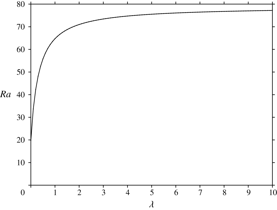
Figure 2. Graph of $Ra$
versus
$Ra$
versus $\unicode[STIX]{x1D706}$
with
$\unicode[STIX]{x1D706}$
with $\unicode[STIX]{x1D706}$
varying in the range 0 to 10, two free surfaces. Here
$\unicode[STIX]{x1D706}$
varying in the range 0 to 10, two free surfaces. Here $Kr=1$
and
$Kr=1$
and $\unicode[STIX]{x1D709}=1$
. The values at the endpoints as shown are
$\unicode[STIX]{x1D709}=1$
. The values at the endpoints as shown are $(Ra,\unicode[STIX]{x1D706})=(19.73921,0)$
and
$(Ra,\unicode[STIX]{x1D706})=(19.73921,0)$
and $(Ra2,\unicode[STIX]{x1D706})=(77.20063,10)$
.
$(Ra2,\unicode[STIX]{x1D706})=(77.20063,10)$
.

Figure 3. Graph of $a^{2}$
versus
$a^{2}$
versus $\unicode[STIX]{x1D709}$
with
$\unicode[STIX]{x1D709}$
with $\unicode[STIX]{x1D709}$
varying in the range 0 to 10, two free surfaces. Here
$\unicode[STIX]{x1D709}$
varying in the range 0 to 10, two free surfaces. Here $Kr=1$
and
$Kr=1$
and $\unicode[STIX]{x1D706}=1$
. The values at the endpoints as shown are
$\unicode[STIX]{x1D706}=1$
. The values at the endpoints as shown are $(a^{2},\unicode[STIX]{x1D709})=(9.448,0)$
and
$(a^{2},\unicode[STIX]{x1D709})=(9.448,0)$
and $(a^{2},\unicode[STIX]{x1D709})=(6.101,10)$
.
$(a^{2},\unicode[STIX]{x1D709})=(6.101,10)$
.
Figure 2 shows that $Ra$
increases rapidly as the Brinkman coefficient
$Ra$
increases rapidly as the Brinkman coefficient $\unicode[STIX]{x1D706}$
increases for
$\unicode[STIX]{x1D706}$
increases for $\unicode[STIX]{x1D706}$
small, and then the growth is less rapid for larger
$\unicode[STIX]{x1D706}$
small, and then the growth is less rapid for larger $\unicode[STIX]{x1D706}$
. This is in agreement with the case of a single-porosity Brinkman material. The variation in the critical wavenumber
$\unicode[STIX]{x1D706}$
. This is in agreement with the case of a single-porosity Brinkman material. The variation in the critical wavenumber $a$
in figures 4–6 is interesting. In our notation, in the single-porosity case replacing
$a$
in figures 4–6 is interesting. In our notation, in the single-porosity case replacing $w\,^{f}$
and
$w\,^{f}$
and $w^{p}$
by
$w^{p}$
by $w$
, instead of (6.5) one has, cf. Rees (Reference Rees2002),
$w$
, instead of (6.5) one has, cf. Rees (Reference Rees2002),
 $$\begin{eqnarray}\displaystyle & \displaystyle -\unicode[STIX]{x1D706}\unicode[STIX]{x1D6E5}^{2}w+\unicode[STIX]{x0394}w-R\unicode[STIX]{x1D6E5}^{\ast }\unicode[STIX]{x1D703}=0, & \displaystyle \nonumber\\ \displaystyle & \displaystyle \unicode[STIX]{x0394}\unicode[STIX]{x1D703}+Rw=0, & \displaystyle \nonumber\end{eqnarray}$$
and instead of (6.6) one finds
 $$\begin{eqnarray}R^{2}={\displaystyle \frac{\unicode[STIX]{x1D706}\unicode[STIX]{x1D6EC}^{3}+\unicode[STIX]{x1D6EC}^{2}}{a^{2}}}.\end{eqnarray}$$
(We stress that Rees (Reference Rees2002) analyses the fixed surface problem.) The presence of the $\unicode[STIX]{x1D706}\unicode[STIX]{x1D6EC}$
term in the denominator of (6.6) changes the
$\unicode[STIX]{x1D706}\unicode[STIX]{x1D6EC}$
term in the denominator of (6.6) changes the $a^{2}$
versus
$a^{2}$
versus $\unicode[STIX]{x1D706}$
behaviour significantly between the one porosity and the bidispersive situation. In the one-porosity case we find for two stress free surfaces that
$\unicode[STIX]{x1D706}$
behaviour significantly between the one porosity and the bidispersive situation. In the one-porosity case we find for two stress free surfaces that $a^{2}$
decreases from
$a^{2}$
decreases from $\unicode[STIX]{x03C0}^{2}$
to
$\unicode[STIX]{x03C0}^{2}$
to $\unicode[STIX]{x03C0}^{2}/2$
as
$\unicode[STIX]{x03C0}^{2}/2$
as $\unicode[STIX]{x1D706}$
increases from 0. In the one-porosity case the critical wavenumber may be obtained analytically and we find
$\unicode[STIX]{x1D706}$
increases from 0. In the one-porosity case the critical wavenumber may be obtained analytically and we find
 $$\begin{eqnarray}a_{cr}^{2}=\{-(\unicode[STIX]{x1D706}\unicode[STIX]{x03C0}^{2}+1)+[(\unicode[STIX]{x1D706}\unicode[STIX]{x03C0}^{2}+1)^{2}+8\unicode[STIX]{x1D706}\unicode[STIX]{x03C0}^{2}(1+\unicode[STIX]{x1D706}\unicode[STIX]{x03C0}^{2})]^{1/2}\}/4\unicode[STIX]{x1D706}.\end{eqnarray}$$
Using Newton’s binomial expansion we find for $\unicode[STIX]{x1D706}$
small,
$\unicode[STIX]{x1D706}$
small,
 $$\begin{eqnarray}a_{cr}^{2}=\unicode[STIX]{x03C0}^{2}-2\unicode[STIX]{x03C0}^{4}\unicode[STIX]{x1D706}+10\unicode[STIX]{x03C0}^{6}\unicode[STIX]{x1D706}^{2}+O(\unicode[STIX]{x1D706}^{3}),\end{eqnarray}$$
which confirms the decrease for $\unicode[STIX]{x1D706}\ll 1$
.
$\unicode[STIX]{x1D706}\ll 1$
.

Figure 4. Graph of $a$
versus
$a$
versus $\log _{10}\unicode[STIX]{x1D706}$
, for
$\log _{10}\unicode[STIX]{x1D706}$
, for $\unicode[STIX]{x1D709}=1,K_{r}=1$
. The solid curve indicates two free surfaces whereas the solid dots are for two fixed surfaces. The minimum on the solid curve is where
$\unicode[STIX]{x1D709}=1,K_{r}=1$
. The solid curve indicates two free surfaces whereas the solid dots are for two fixed surfaces. The minimum on the solid curve is where $a=2.7207,\unicode[STIX]{x1D706}=0.17$
, and the maximum value displayed for fixed surfaces is
$a=2.7207,\unicode[STIX]{x1D706}=0.17$
, and the maximum value displayed for fixed surfaces is $a=3.2088,\unicode[STIX]{x1D706}=0.01$
.
$a=3.2088,\unicode[STIX]{x1D706}=0.01$
.

Figure 5. Graph of $a$
versus
$a$
versus $\log _{10}\unicode[STIX]{x1D706}$
, for
$\log _{10}\unicode[STIX]{x1D706}$
, for $\unicode[STIX]{x1D709}=0.1316,K_{r}=2322$
. The solid curve indicates two free surfaces whereas the solid dots are for two fixed surfaces. The minimum on the solid curve is where
$\unicode[STIX]{x1D709}=0.1316,K_{r}=2322$
. The solid curve indicates two free surfaces whereas the solid dots are for two fixed surfaces. The minimum on the solid curve is where $a=2.24586,\unicode[STIX]{x1D706}=3.46$
, and the maximum value displayed for fixed surfaces is
$a=2.24586,\unicode[STIX]{x1D706}=3.46$
, and the maximum value displayed for fixed surfaces is $a=3.239,$ $\unicode[STIX]{x1D706}\in [0.005,0.006]$
.
$\unicode[STIX]{x1D706}\in [0.005,0.006]$
.

Figure 6. Graph of $a$
versus
$a$
versus $\log _{10}\unicode[STIX]{x1D706}$
, for
$\log _{10}\unicode[STIX]{x1D706}$
, for $\unicode[STIX]{x1D709}=0.01515,K_{r}=25$
. The solid curve indicates two free surfaces whereas the solid dots are for two fixed surfaces. The minimum on the solid curve is where
$\unicode[STIX]{x1D709}=0.01515,K_{r}=25$
. The solid curve indicates two free surfaces whereas the solid dots are for two fixed surfaces. The minimum on the solid curve is where $a=2.43084,\unicode[STIX]{x1D706}=0.33$
, and the maximum value displayed for fixed surfaces is
$a=2.43084,\unicode[STIX]{x1D706}=0.33$
, and the maximum value displayed for fixed surfaces is $a=3.234,$ $\unicode[STIX]{x1D706}\in [0.004,0.006]$
.
$\unicode[STIX]{x1D706}\in [0.004,0.006]$
.
In the bidisperse case figures 4–6 show for two free surfaces a clear decrease then increase as $\unicode[STIX]{x1D706}$
increases for small
$\unicode[STIX]{x1D706}$
increases for small $\unicode[STIX]{x1D706}$
. The initial decrease may be verified by an asymptotic analysis from (6.6). If we form
$\unicode[STIX]{x1D706}$
. The initial decrease may be verified by an asymptotic analysis from (6.6). If we form $\unicode[STIX]{x2202}R^{2}/\unicode[STIX]{x2202}a^{2}$
from (6.6) and equate to zero and then solve the resulting equation by expanding
$\unicode[STIX]{x2202}R^{2}/\unicode[STIX]{x2202}a^{2}$
from (6.6) and equate to zero and then solve the resulting equation by expanding $a^{2}$
as a power series in
$a^{2}$
as a power series in $\unicode[STIX]{x1D706}$
then for
$\unicode[STIX]{x1D706}$
then for $0<\unicode[STIX]{x1D706}\ll 1$
we find
$0<\unicode[STIX]{x1D706}\ll 1$
we find
 $$\begin{eqnarray}a^{2}=\unicode[STIX]{x03C0}^{2}-X_{1}\unicode[STIX]{x1D706}+O(\unicode[STIX]{x1D706}^{2}),\quad \text{where }X_{1}=2\unicode[STIX]{x03C0}^{6}\left[{\displaystyle \frac{K_{r}^{2}+4K_{r}\unicode[STIX]{x1D709}+4\unicode[STIX]{x1D709}^{2}}{(K_{r}+K_{r}\unicode[STIX]{x1D709}+\unicode[STIX]{x1D709})(1+K_{r}+4\unicode[STIX]{x1D709})}}\right].\end{eqnarray}$$
In fact, when $K_{r}=1,\unicode[STIX]{x1D709}=1$
the minimum value is
$K_{r}=1,\unicode[STIX]{x1D709}=1$
the minimum value is $(a^{2},\unicode[STIX]{x1D706})=(7.402,0.17)$
whereas for
$(a^{2},\unicode[STIX]{x1D706})=(7.402,0.17)$
whereas for $K_{r}=5,\unicode[STIX]{x1D709}=0.01$
the minimum is at
$K_{r}=5,\unicode[STIX]{x1D709}=0.01$
the minimum is at $(a^{2},\unicode[STIX]{x1D706})=(6.953,0.15)$
. Thus the presence of micropores is changing the behaviour of the cell shape. When micropores are present and
$(a^{2},\unicode[STIX]{x1D706})=(6.953,0.15)$
. Thus the presence of micropores is changing the behaviour of the cell shape. When micropores are present and $\unicode[STIX]{x1D706}$
is small the cell shape increases in width (aspect ratio) as
$\unicode[STIX]{x1D706}$
is small the cell shape increases in width (aspect ratio) as $\unicode[STIX]{x1D706}$
increases, reaching a maximum and then decreasing again. The wavenumber variation for
$\unicode[STIX]{x1D706}$
increases, reaching a maximum and then decreasing again. The wavenumber variation for $\unicode[STIX]{x1D706}$
small is, however, very different from the free–free case. We see that in tables 3 and 4 when the surfaces are fixed then the wavenumber has a maximum in
$\unicode[STIX]{x1D706}$
small is, however, very different from the free–free case. We see that in tables 3 and 4 when the surfaces are fixed then the wavenumber has a maximum in $\unicode[STIX]{x1D706}$
. This is exactly the opposite behaviour to the free–free situation. This behaviour is, however, in agreement with the findings of Rees (Reference Rees2002) in the single-porosity case. He also predicts a rise then decrease in
$\unicode[STIX]{x1D706}$
. This is exactly the opposite behaviour to the free–free situation. This behaviour is, however, in agreement with the findings of Rees (Reference Rees2002) in the single-porosity case. He also predicts a rise then decrease in $a$
as
$a$
as $\unicode[STIX]{x1D706}$
decreases. We have checked the behaviour of the critical value of
$\unicode[STIX]{x1D706}$
decreases. We have checked the behaviour of the critical value of $a$
in the free–free single-porosity case and it is as in figures 4–6. We have computed the critical Rayleigh number and wavenumber for various other combinations of possible realistic values of parameter values and we always see the same type of behaviour as
$a$
in the free–free single-porosity case and it is as in figures 4–6. We have computed the critical Rayleigh number and wavenumber for various other combinations of possible realistic values of parameter values and we always see the same type of behaviour as $\unicode[STIX]{x1D706}$
varies.
$\unicode[STIX]{x1D706}$
varies.
Table 2. Critical values of $Ra$
and
$Ra$
and $a$
for quoted values of
$a$
for quoted values of $\unicode[STIX]{x1D706}$
, two fixed surfaces. Columns 2 and 3 are for
$\unicode[STIX]{x1D706}$
, two fixed surfaces. Columns 2 and 3 are for $K_{r}=1$
,
$K_{r}=1$
, $\unicode[STIX]{x1D709}=1$
, while columns 4 and 5 are for
$\unicode[STIX]{x1D709}=1$
, while columns 4 and 5 are for $K_{r}=5$
,
$K_{r}=5$
, $\unicode[STIX]{x1D709}=0.01$
.
$\unicode[STIX]{x1D709}=0.01$
.
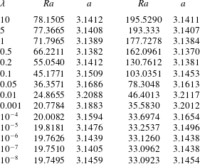
Table 3. Critical values of $Ra$
and
$Ra$
and $a$
for quoted values of
$a$
for quoted values of $\unicode[STIX]{x1D706}$
, two fixed surfaces. Columns 2 and 3 are for
$\unicode[STIX]{x1D706}$
, two fixed surfaces. Columns 2 and 3 are for $K_{r}=1$
,
$K_{r}=1$
, $\unicode[STIX]{x1D709}=1$
, while columns 4 and 5 are for
$\unicode[STIX]{x1D709}=1$
, while columns 4 and 5 are for $K_{r}=5$
,
$K_{r}=5$
, $\unicode[STIX]{x1D709}=0.01$
.
$\unicode[STIX]{x1D709}=0.01$
.
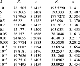
Table 4. Critical values of $Ra$
and
$Ra$
and $a$
for quoted values of
$a$
for quoted values of $\unicode[STIX]{x1D706}$
, two fixed surfaces. Columns 2 and 3 are for
$\unicode[STIX]{x1D706}$
, two fixed surfaces. Columns 2 and 3 are for $K_{r}=2322$
,
$K_{r}=2322$
, $\unicode[STIX]{x1D709}=0.1316$
, while columns 4 and 5 are for
$\unicode[STIX]{x1D709}=0.1316$
, while columns 4 and 5 are for $K_{r}=25$
,
$K_{r}=25$
, $\unicode[STIX]{x1D709}=0.01515$
.
$\unicode[STIX]{x1D709}=0.01515$
.
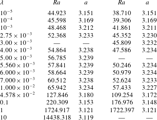
Table 5. Critical values of $Ra$
and
$Ra$
and $a$
for quoted values of
$a$
for quoted values of $Kr$
, two fixed surfaces. Columns 2 and 3 are for
$Kr$
, two fixed surfaces. Columns 2 and 3 are for $\unicode[STIX]{x1D706}=0.04578$
,
$\unicode[STIX]{x1D706}=0.04578$
, $\unicode[STIX]{x1D709}=0.1316$
, while columns 4 and 5 are for
$\unicode[STIX]{x1D709}=0.1316$
, while columns 4 and 5 are for $\unicode[STIX]{x1D706}=0.00275$
,
$\unicode[STIX]{x1D706}=0.00275$
, $\unicode[STIX]{x1D709}=0.01515$
.
$\unicode[STIX]{x1D709}=0.01515$
.
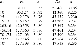
Table 6. Critical values of the wavenumber $a$
for quoted values of
$a$
for quoted values of $Kr$
, two free surfaces. Columns 2 and 3 are for
$Kr$
, two free surfaces. Columns 2 and 3 are for $\unicode[STIX]{x1D706}=0.04578$
,
$\unicode[STIX]{x1D706}=0.04578$
, $\unicode[STIX]{x1D709}=0.1316$
, while columns 4 and 5 are for
$\unicode[STIX]{x1D709}=0.1316$
, while columns 4 and 5 are for $\unicode[STIX]{x1D706}=0.00275$
,
$\unicode[STIX]{x1D706}=0.00275$
, $\unicode[STIX]{x1D709}=0.01515$
.
$\unicode[STIX]{x1D709}=0.01515$
.

In figure 4 the maximum and minimum values for the fixed and free cases have reasonably close values of $\unicode[STIX]{x1D706}$
, but these are when
$\unicode[STIX]{x1D706}$
, but these are when $K_{r}=1,\unicode[STIX]{x1D709}=1$
. For
$K_{r}=1,\unicode[STIX]{x1D709}=1$
. For $K_{r}$
and
$K_{r}$
and $\unicode[STIX]{x1D709}$
values which we have calculated for possible real bidisperse materials figures 5 and 6 show that the maximum in
$\unicode[STIX]{x1D709}$
values which we have calculated for possible real bidisperse materials figures 5 and 6 show that the maximum in $\unicode[STIX]{x1D706}$
for the fixed surface problem is in the range of realistic values. The corresponding minima in
$\unicode[STIX]{x1D706}$
for the fixed surface problem is in the range of realistic values. The corresponding minima in $\unicode[STIX]{x1D706}$
for the free surface situation are for larger values of
$\unicode[STIX]{x1D706}$
for the free surface situation are for larger values of $\unicode[STIX]{x1D706}$
.
$\unicode[STIX]{x1D706}$
.
The variations of $Ra$
and
$Ra$
and $a$
in
$a$
in $\unicode[STIX]{x1D709}$
are given in tables 7 and 8 with potentially realistic values of parameters. For fixed surfaces the situation of the behaviour of
$\unicode[STIX]{x1D709}$
are given in tables 7 and 8 with potentially realistic values of parameters. For fixed surfaces the situation of the behaviour of $a$
is not clear. In table 7, for
$a$
is not clear. In table 7, for $\unicode[STIX]{x1D706}=4.578\times 10^{-2}$
and
$\unicode[STIX]{x1D706}=4.578\times 10^{-2}$
and $K_{r}=25$
or 2322 the critical wavenumber
$K_{r}=25$
or 2322 the critical wavenumber $a$
always increases as
$a$
always increases as $\unicode[STIX]{x1D709}$
increases. However, from table 7, for
$\unicode[STIX]{x1D709}$
increases. However, from table 7, for $\unicode[STIX]{x1D706}=2.75\times 10^{-3}$
and
$\unicode[STIX]{x1D706}=2.75\times 10^{-3}$
and $K_{r}=25$
or 2322,
$K_{r}=25$
or 2322, $a$
always decreases. For the free surface case
$a$
always decreases. For the free surface case $a$
is found to increase in all four cases as seen in table 9.
$a$
is found to increase in all four cases as seen in table 9.
Table 7. Critical values of $Ra$
and
$Ra$
and $a$
for quoted values of
$a$
for quoted values of $\unicode[STIX]{x1D709}$
, two fixed surfaces. Columns 2 and 3 are for
$\unicode[STIX]{x1D709}$
, two fixed surfaces. Columns 2 and 3 are for $\unicode[STIX]{x1D706}=0.04578$
,
$\unicode[STIX]{x1D706}=0.04578$
, $K_{r}=25$
, while columns 4 and 5 are for
$K_{r}=25$
, while columns 4 and 5 are for $\unicode[STIX]{x1D706}=0.04578$
,
$\unicode[STIX]{x1D706}=0.04578$
, $Kr=2322$
.
$Kr=2322$
.

Table 8. Critical values of $Ra$
and
$Ra$
and $a$
for quoted values of
$a$
for quoted values of $\unicode[STIX]{x1D709}$
, two fixed surfaces. Columns 2 and 3 are for
$\unicode[STIX]{x1D709}$
, two fixed surfaces. Columns 2 and 3 are for $\unicode[STIX]{x1D706}=0.00275$
,
$\unicode[STIX]{x1D706}=0.00275$
, $K_{r}=25$
, while columns 4 and 5 are for
$K_{r}=25$
, while columns 4 and 5 are for $\unicode[STIX]{x1D706}=0.00275$
,
$\unicode[STIX]{x1D706}=0.00275$
, $Kr=2322$
.
$Kr=2322$
.

Table 9. Critical values of the wavenumber $a$
for quoted values of
$a$
for quoted values of $\unicode[STIX]{x1D709}$
, two free surfaces. Column 2 is for
$\unicode[STIX]{x1D709}$
, two free surfaces. Column 2 is for $\unicode[STIX]{x1D706}=0.04578$
,
$\unicode[STIX]{x1D706}=0.04578$
, $K_{r}=25$
, column 3 is for
$K_{r}=25$
, column 3 is for $\unicode[STIX]{x1D706}=0.04578$
,
$\unicode[STIX]{x1D706}=0.04578$
, $Kr=2322$
, column 4 is for
$Kr=2322$
, column 4 is for $\unicode[STIX]{x1D706}=0.00275$
,
$\unicode[STIX]{x1D706}=0.00275$
, $K_{r}=25$
and column 5 is for
$K_{r}=25$
and column 5 is for $\unicode[STIX]{x1D706}=0.00275$
,
$\unicode[STIX]{x1D706}=0.00275$
, $Kr=2322$
.
$Kr=2322$
.

9 Conclusions
We have presented a model for thermal convection in a dual-porosity (bidisperse) porous medium which allows for the macropermeability to be relatively large compared to the micropermeability. The behaviour of the critical Rayleigh number, $Ra$
, and critical wavenumber,
$Ra$
, and critical wavenumber, $a$
, depends on three parameters,
$a$
, depends on three parameters, $\unicode[STIX]{x1D706}$
,
$\unicode[STIX]{x1D706}$
, $\unicode[STIX]{x1D709}$
and
$\unicode[STIX]{x1D709}$
and $K_{r}$
given in (6.3). We observe that these non-dimensional parameters represent the Brinkman coefficient, the mass transfer coefficient between the macro and microphases and
$K_{r}$
given in (6.3). We observe that these non-dimensional parameters represent the Brinkman coefficient, the mass transfer coefficient between the macro and microphases and $K_{r}=K_{f}/K_{p}$
represents the ratio of macropermeability to micropermeability, respectively. We have calculated a possible selection of values for each of these parameters which may represent real materials.
$K_{r}=K_{f}/K_{p}$
represents the ratio of macropermeability to micropermeability, respectively. We have calculated a possible selection of values for each of these parameters which may represent real materials.
In all cases the critical Rayleigh number, $Ra$
, of global nonlinear stability increases as
$Ra$
, of global nonlinear stability increases as $\unicode[STIX]{x1D709},\unicode[STIX]{x1D706}$
or
$\unicode[STIX]{x1D709},\unicode[STIX]{x1D706}$
or $K_{r}$
increase. Since increasing
$K_{r}$
increase. Since increasing $Ra$
means the layer becomes more stable, then if one is interested in insulation a higher value of
$Ra$
means the layer becomes more stable, then if one is interested in insulation a higher value of $Ra$
is desirable. Alternatively, if heat transfer is required we want convection to occur to aid this transfer and a smaller value of
$Ra$
is desirable. Alternatively, if heat transfer is required we want convection to occur to aid this transfer and a smaller value of $Ra$
is preferable. Thus, for insulation one should ensure
$Ra$
is preferable. Thus, for insulation one should ensure $\unicode[STIX]{x1D709},\unicode[STIX]{x1D706}$
and
$\unicode[STIX]{x1D709},\unicode[STIX]{x1D706}$
and $K_{r}$
are as large as possible, whereas if one requires rapid heat transfer the smallest values of these parameters are preferred.
$K_{r}$
are as large as possible, whereas if one requires rapid heat transfer the smallest values of these parameters are preferred.
The wavenumber behaviour is very different when fixed surface boundary conditions are employed as to when free ones are utilized. Since we expect fixed conditions in normal circumstances we deal with this. The behaviour with respect to the Brinkman coefficient is such that the critical wavenumber $a$
increases to a maximum in
$a$
increases to a maximum in $\unicode[STIX]{x1D706}$
and then decreases. This means that the aspect ratio of the cells decrease then increase with increasing
$\unicode[STIX]{x1D706}$
and then decreases. This means that the aspect ratio of the cells decrease then increase with increasing $\unicode[STIX]{x1D706}$
.
$\unicode[STIX]{x1D706}$
.
For the values we have investigated, as $K_{r}$
increases
$K_{r}$
increases $a$
increases, but the variation is small over the range of estimated parameter values.
$a$
increases, but the variation is small over the range of estimated parameter values.
The variation of $a$
in
$a$
in $\unicode[STIX]{x1D709}$
appears to depend critically on what values the Brinkman parameter
$\unicode[STIX]{x1D709}$
appears to depend critically on what values the Brinkman parameter $\unicode[STIX]{x1D706}$
and the permeability ratio
$\unicode[STIX]{x1D706}$
and the permeability ratio $K_{r}$
have. The non-dimensional momentum transfer coefficient
$K_{r}$
have. The non-dimensional momentum transfer coefficient $\unicode[STIX]{x1D709}$
displays both increasing or decreasing behaviour and the critical wavenumber appears to depend precisely on what values are assigned to
$\unicode[STIX]{x1D709}$
displays both increasing or decreasing behaviour and the critical wavenumber appears to depend precisely on what values are assigned to $\unicode[STIX]{x1D706}$
and
$\unicode[STIX]{x1D706}$
and $K_{r}$
.
$K_{r}$
.
Acknowledgements
The work of M.G. was performed under the auspices of the National Group of Mathematical Physics GNFM-INdAM, while that of B.S. was supported by an Emeritus Fellowship of the Leverhulme Trust, EM-2019-022/9. We are indebted to four anonymous referees for their incisive critiscism of a previous version of this work. Their comments have led to very substantial improvements in the paper.
Declaration of interests
The authors report no conflict of interest.


 Open access