


1. Introduction
Coalescence is an enticing phenomenon for study by the fluid dynamicist as it involves several of the major force contributions seen in the field namely capillary, viscous, inertial and gravity forces. The study of coalescing fluids has allowed for advances in microfluidics (Prakash & Gershenfeld Reference Prakash and Gershenfeld2007), additive manufacturing in microgravity (Huang et al. Reference Huang, Qi, Luo, Zhao and Yi2020), bioprinting of living tissue (Murphy & Atala Reference Murphy and Atala2014), the inkjet printing of electronics (Zhu, Wang & Zhu Reference Zhu, Wang and Zhu2020) and even the study of natural phenomena such as rain (D'Adderio, Porcù & Tokay Reference D'Adderio, Porcù and Tokay2018). Coalescence can largely be separated into drop–drop coalescence (Yuan et al. Reference Yuan, He, Fang, Bao and Liu2015; Duchemin, Eggers & Josserand Reference Duchemin, Eggers and Josserand2003; Gebauer et al. Reference Gebauer, Villwock, Kraume and Bart2016), bubble coalescence (Liu et al. Reference Liu, Manica, Liu, Klaseboer, Xu and Xie2019; Cui et al. Reference Cui, Wang, Wang and Zhang2016; Feng et al. Reference Feng, Li, Bao, Cai and Gao2016; Han et al. Reference Han, Li, Zhang and Wang2016), the study of onset (Neitzel & Dell'Aversana Reference Neitzel and Dell'Aversana2002; Geri et al. Reference Geri, Keshavarz, McKinley and Bush2017) and drop–planar coalescence (Politova et al. Reference Politova, Tcholakova, Tsibranska, Denkov and Muelheims2017; Zhang et al. Reference Zhang, Jiang, Brunello, Fu, Zhu, Ma and Li2019; Kirar et al. Reference Kirar, Alvarenga, Kolhe, Biswas and Chandra Sahu2020) which is the focus of this study. At planar surfaces coalescence can occur in two ways: partial or full coalescence. Full coalescence is characterized by complete drainage of the droplet into the free surface while partial coalescence produces a smaller so-called ‘daughter’ droplet (Kavehpour Reference Kavehpour2015).
Lord Rayleigh first characterized the breakup of fluid columns or jets to droplets, a mechanism driving the partial coalescence process, back in 1878 (Rayleigh Reference Rayleigh1878). This analysis serves as the foundation for work through the 20th century continuing even through to the present day. The importance of viscosity in determining the parameters of a coalescence event and has been studied at planar surfaces by Gillespie & Rideal (Reference Gillespie and Rideal1956) whose work focused on the drainage time of the coalescing droplets as well as the condition for droplet rupture, finding it occurred when film at the drop–surface interface was  $10^{-5}$ to $10^{-6}$ m thick. A foundational study of planar coalescence, including partial coalescence can be found in the well-known works by Charles and Mason, which serve as a basis for much of the subsequent work (Charles & Mason Reference Charles and Mason1960a,Reference Charles and Masonb). These studies were conducted in a viscous quiescent fluid with the first taking a hydrodynamic approach to study the onset of coalescence at a planar surface as well as the coalescing time. The second paper focuses on partial coalescence, on which this paper will focus as well, comparing the ratio of droplet radii $r_i = R_2/R_1$, where $R_1$ is the father droplet radius and $R_2$ is the radius of the daughter droplet, to the viscosity ratio of the droplet fluid and quiescent fluid. This work also established a framework for the production of a daughter droplet using linear stability analysis to find the amplitude for the most dominant wavelength successful in producing the droplet using the method established by Rayleigh. Tomotika (Reference Tomotika1935) established a working model for the parameter ${\rm \pi} /Z_0$, or the ratio of circumference to optimum wavelength, which was found to be about 0.68 by Charles and Mason for mercury, the substance that is most comparable to the liquid metal chosen for our study. Using a simplified model they derived a readily usable equation for this parameter given by
 \begin{equation} Z_0= (\tfrac{3}{2}r_i^{{-}3})^{1/2}. \end{equation}
 Tomotika's study created a theoretical framework that produced a model for  ${\rm \pi} /Z_0$ as a function of the viscosity ratio $p=\mu _o/\mu _i$, where $\mu _i$ and $\mu _o$ are the inner and outer viscosities, respectively, for a range of $0.001 \leq p \leq 100$. The result of this analysis was a model that predicted a maximum value out a viscosity ratio of $p=0.28$ with the tail ends reaching 0 as the viscosity ratio tended towards 0, the case of an inviscid inner fluid, or towards infinity, for an inviscid outer fluid. While this work is often cited for drops coalescing in a quiescent fluid, many studies conducted since have produced data that do not match Tomotika's model (Charles & Mason Reference Charles and Mason1960b; Aryafar & Kavehpour Reference Aryafar and Kavehpour2006). This indicates a more complicated relationship between the propensity to partially coalesce, the parameter $Z_0$ and by extension $r_i$, than the viscosity ratio alone. For example Fedorchenko & Wang (Reference Fedorchenko and Wang2004) conducted experiments of droplets impacting on liquid surfaces and observed a partial coalescence cascade including bouncing of the daughter droplets. They found a regime defined by the dimensionless capillary length $l_{c}^{*} = l_c/D$ where $l_c$ is the capillary length $l_c =\sqrt {\sigma / \Delta \rho g}$ and D is the droplet diameter, g is the acceleration due to gravity and $\Delta\rho$ is the density difference between the inner and outer fluids. They determined the regime for partial coalescence effects to begin at $l_{c}^{*2}>1$ and end at a critical value of 28.3. While their experiments are complicated by the effects of the droplet impact, they indicate the importance of capillary forces in the dynamics of the generation and subsequent behaviour of the secondary droplets. This relationship can also be interpreted as the regime where $We<2Fr$ and $0.1< Fr<200$, where $We$ and $Fr$ are the Weber, $We = \rho V^2 D / \sigma$, and Froude, $Fr = V / \sqrt {g D}$ numbers, respectively, emphasizing the important contribution of capillarity in overcoming gravitational body force effects. Here, and throughout this manuscript, $\rho$, $\mu$, $\sigma$, g, $V$ and $D$ will refer to the density (kg m $^{-3}$), dynamic viscosity (Pa s), surface/interfacial tension (N m $^{-1}$), acceleration due to gravity (g = 9.81 m s−1), droplet velocity (m s $^{-1}$) and characteristic length (m), usually the droplet diameter, and refer to the inner fluid unless stated otherwise.
The Ohnesorge number,  $Oh = \mu / \sqrt {\rho \sigma D}$, is a parameter that has seen a great deal of focus for the limit of partial coalescence. The importance of $Oh$ with respect to applications such as inkjet printing, which involve both coalescence and droplet breakup which is dynamically very similar to partial coalescence, has been noted by many works such as the study by Derby (Reference Derby2010). This work sets a limit of $Oh < 1$ for droplet breakup, beyond which the fluid is too viscous. This becomes intuitive if one assumes that capillary force is a driving force in the breakup process while viscous forces serve to stabilize the fluid column.
Blanchette & Bigioni (Reference Blanchette and Bigioni2006) focused on the Ohnesorge number as a criterion for pinch off when the Bond number,  $Bo = \Delta \rho g R_1/ \sigma$, was sufficiently small. Through both simulation and experiments using ethanol they found a critical value for the Ohnesorge number $Oh = 0.026\pm 0.001$ when the Bond number, $Bo$, was less than 0.1. Above this critical $Oh$ the authors assert that only full coalescence can occur. Previous work by our group (Aryafar & Kavehpour Reference Aryafar and Kavehpour2006) utilizing a number of liquids coalescing in planar surfaces in air showed coalescence occurring up to the $Oh < 1$ threshold with the droplet ratio obeying the following relationship: $r_i=(1-0.75\alpha -0.75\beta Oh)^{1/3}$, where $\alpha =1.13$ and $\beta =0.25$ are empirically determined constants. This comes from considering that inertial effects dominate until $Oh \xrightarrow {} 1^-$ at which point viscous forces begin to dominate which matches the conclusions that Ray, Biswas & Sharma (Reference Ray, Biswas and Sharma2010) reached as well.
The time scales of coalescence are also of interest where viscous and inertial regimes are differentiated, with some literature naming a third regime where inertia is important. Inviscid theory predicts that coalescence time will scale as  $t \sim R^{3/2}$ due to the inertial time scale taking the form $t_i = \sqrt {\rho R_1^3 / \sigma }$ (Thoroddsen & Takehara Reference Thoroddsen and Takehara2000). Xia, He & Zhang (Reference Xia, He and Zhang2019) explored the effect of crossing over from the viscous regime to the inertial regime by studying the relative time scales for each type of behaviour, using $Oh$ as a basis for differentiating them. This work was able to affirm that in the inertial regime, the coalescence time scales with the radius to the power of 1/2 while in the viscous regime coalescence time scales linearly with the radius. This built upon previous work such as that by Paulsen et al. (Reference Paulsen, Burton, Nagel, Appathurai, Harris and Basaran2012), which also included a third regime in which both viscous and inertial forces are important. The scaling of $t \sim R$ for viscous regime and $t \sim R^{3/2}$ for the inertial/capillary regime are generally the accepted scaling parameters for the coalescence process. These works serve to affirm the importance of the Ohnesorge number in properly stratifying the dynamic regimes of coalescence.
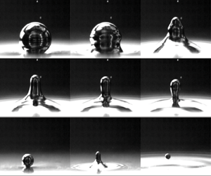
For this study we will build on our work previously exploring the phenomenon of a bouncing, partial coalescing droplet in air (Honey & Kavehpour Reference Honey and Kavehpour2006) and develop a dynamical model including viscous effects in a quiescent fluid. The partial coalescence process imparts a downward velocity  $V_0$ on the generated daughter droplet due to capillary and body forces. This process is detailed in figure 1 and modified from Honey's work to include buoyancy effects.
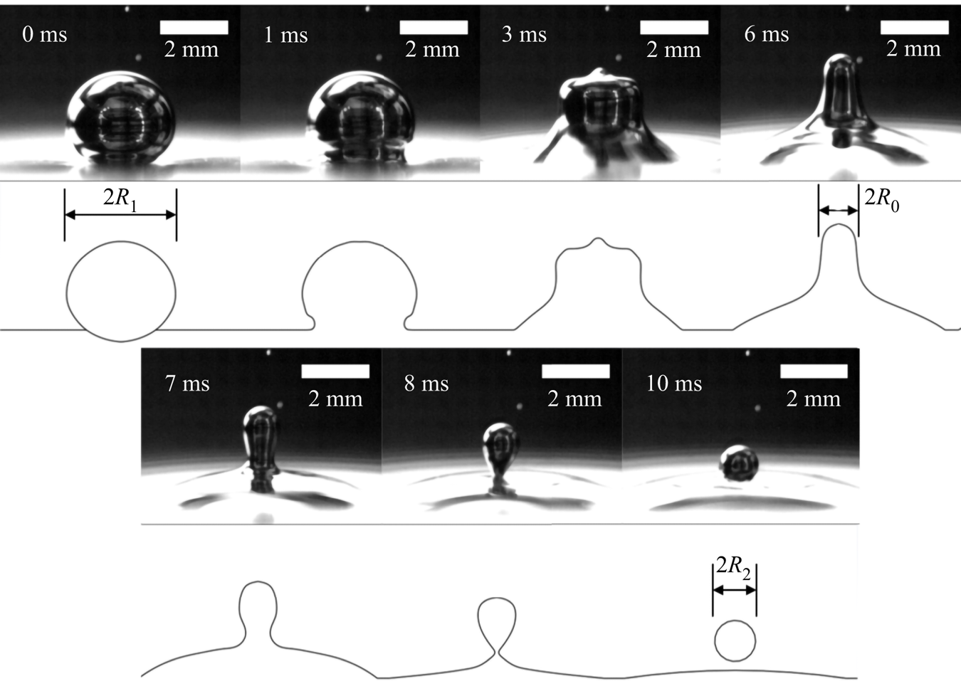
Figure 1. Partial coalescence generation of the daughter droplet.
As shown in the figure, first the droplet of radius  $R_1$ resides on the interface, supported by a thin lubrication layer of the surrounding NaOH. At 1 ms the capillary wave can be seen initiating from the base and continues upward, as shown in the image at 3 ms. The fluid forms a column of diameter $2R_0$ where $R_0= R_1 \sqrt {2 r_i^3 / 3}$, which is found by equating the volume of the daughter droplet to the fluid column (Charles & Mason Reference Charles and Mason1960b). This column will then begin to breakup per Rayleigh's model with the pinch-off at the neck first, shown in figure 1 at 7 ms. At first the neck begins at radius $R_0$ but pinches off over a time as described by Clanet & Lasheras (Reference Clanet and Lasheras1999). During this time capillary and gravity forces both act downward on the droplet. We can write an equation for the force balance on the fluid mass that will become the eventual daughter droplet as follows:
 \begin{equation} \left(m \frac{\textrm{d}V}{\textrm{d}t} \right)_{drop}= F_{grav} + F_{cap} = \frac{4}{3} \Delta \rho {\rm \pi}R_2^3 g + 2 {\rm \pi}R(t) \sigma, \end{equation}
where  $\Delta \rho = \rho _i - \rho _o$, the difference between the inner and outer fluid densities and the neck width $R(t)$ is
 \begin{equation} R(t) = R_0(1- \textrm{e}^{{(t-t_i)}/{t_i}}), \end{equation}
which is given by the aforementioned work by Clanet and Lasheras. The neck continues to shrink, as shown in figure 1 in the sixth image, over a period governed by the inertial time scale  $t_{i} = \sqrt {\rho R_1^3 / \sigma }$. The final image in the figure shows the daughter droplet of radius $R_2$ which is generated with an initial downward velocity of $V_0$. The size is related to $R_1$ by
 \begin{equation} R_2 = r_i R_1. \end{equation}
 By integrating equation (1.2) over  $t_i$ with initial condition $V(0) = 0$ the equation for the downward velocity $V_0$ can be obtained
 \begin{equation} V_0 = \frac{1}{e} \sqrt{\frac{3 \sigma}{2 \rho r_i^3 R_1}} +\frac{\Delta \rho }{\rho} g \sqrt{\frac{\rho R_1^3}{\sigma}}. \end{equation}
 Equation (1.5) will serve as an important initial condition for the model we will use for bouncing droplets in a viscous medium. Note that this model relies on Rayleigh's inviscid model for break-up. While a viscous dispersion relation developed by Chandrasekhar (Reference Chandrasekhar2013) does exist, it can be unwieldy and yields very similar results to the inviscid model (Pekker Reference Pekker2018). Furthermore, this work will focus exclusively on low Ohnesorge numbers  $Oh \ll 1$ so the inviscid model will suffice. Ray et al. (Reference Ray, Biswas and Sharma2010) studied partial coalescence in a two liquid system using a combination of numerical and experimental techniques. They too found that the interfacial and inertial characteristics are the primary relevant parameters for describing the generation of daughter droplets.
1.1. Room temperature liquid metal
Gallium based alloys have become popular in recent years due to several desirable material properties notably their low melting points, low toxicity and high thermal and electrical conductivities (Ivanoff, Ivanoff & Hottel Reference Ivanoff, Ivanoff and Hottel2012; Dickey Reference Dickey2014). The properties of these alloys make them ideal candidates for applications such as stretchable electronics (Dickey Reference Dickey2017), practical chemistry (Daeneke et al. Reference Daeneke, Khoshmanesh, Mahmood, De Castro, Esrafilzadeh, Barrow, Dickey and Kalantar-Zadeh2018) and microfluidics (Khoshmanesh et al. Reference Khoshmanesh, Tang, Zhu, Schaefer, Mitchell, Kalantar-Zadeh and Dickey2017). Here, we seek to use a specific formulation consisting of 68.5 % gallium, 21.5 % indium and 10 % tin, known commercially as Galinstan and is commercially available from Geratherm Medical AG in Germany with RG Medical Diagnostics distributing in the US. The material properties for this formulation are listed in table 1. This material is a eutectic alloy which remains liquid well below room temperature, solidifying at 10  $^\circ$C (Tang et al. Reference Tang, Tabor, Kalantar-Zadeh and Dickey2021). This combined with the negligible vapour pressure and high boiling point make this room temperature liquid metal (RTLM) an ideal candidate for many practical and laboratory applications.
Table 1. Gallium Based Eutectic Material Properties. Composition: Ga: 68.5 % In : 21.5 % Sn: 10 % (Geratherm & Geschwenda Reference Geratherm and Geschwenda2006; Liu, Sen & Kim Reference Liu, Sen and Kim2011; Handschuh-Wang et al. Reference Handschuh-Wang, Chen, Zhu and Zhou2018; Kocourek Reference Kocourek2008; Tang et al. Reference Tang, Tabor, Kalantar-Zadeh and Dickey2021).

While this eutectic is often compared favourably with mercury in terms of its usefulness, like mercury there exists a significant challenge when working with the material. For mercury the toxicity is often cited as a primary challenge, for gallium alloys, the problem is oxidation at the fluid surface. While some have found uses or workarounds for this surface layer such as Ladd et al. (Reference Ladd, So, Muth and Dickey2013), who were able to exploit the stiffness introduced by the skin to create free standing structures, many investigators either lose interest in the material or seek a workaround. Alloys containing gallium will react with ambient oxygen to produce gallium (III) oxide or gallium (I) oxide at the surface of the liquid (Kim et al. Reference Kim, Thissen, Viner, Lee, Choi, Chabal and Lee2013). This layer is extremely thin, of the order of  $\sim$5 Å and insulates the bulk fluid quite well from additional oxidation (Regan et al. Reference Regan, Tostmann, Pershan, Magnussen, DiMasi, Ocko and Deutsch1997). Despite being very thin the oxide layer significantly impacts the dynamics of the moving fluid, particularly the wetting, spreading and other capillary behaviours. Jia et al. (Reference Jia, Yang, Zhang and Ni2019) showed that the presence of the oxide layer inhibits Plateau–Rayleigh instability breakup of jets which, as mentioned previously, is important for the partial coalescence process. The surface tension of this RTLM is usually reported as 0.718 N m $^{-1}$, but this is a facet of the measurement technique and other methods have found it to be 0.517 N m $^{-1}$ $\pm$6 % (Kocourek Reference Kocourek2008). This indicates that the presence of the oxide layer must be attended to in order to properly study the phenomenon.
Fortunately, a solution exists to study capillary effects with RTLMs through either the prevention of oxidation through the use of isolation and inert gasses such as nitrogen or argon. The difficulty here is that oxidation may have occurred before the sample is isolated. In order to ensure that the oxide layer is not present at any time, the layer may be reduced using a strong acid or base. The most commonly used candidates are hydrochloric acid (HCl) and sodium hydroxide (NaOH). Table 1 depicts several of the values of surface or interfacial tension (IFT) reported in the literature. Handschuh-Wang et al. (Reference Handschuh-Wang, Chen, Zhu and Zhou2018) studied the IFT of Galinstan in NaOH and HCl as a function or molarity and time. For HCl, even in higher concentrations, the IFT took at least 1 min to converge to a steady value. For NaOH in concentrations of 1M the value of IFT converged to  $0.4042~\textrm {N~m}^{-1} \pm 0.0032$ N m $^{-1}$ very quickly and as such we chose 1 M NaOH in water as the quiescent fluid for these experiments. We also confirmed the IFT value of the RTLM with 1 M NaOH with a procedure detailed in § 2.
2. Experimental methods
The basic experimental set-up is depicted in figure 2. All components were mounted to an optical table to ensure a level test space and minimize vibration. This is particularly important as the droplets are prone to skate out of frame or focus if there are errors in levelling or too much ambient vibration. A high powered LED light source provided illumination and an optical diffuser was used to ensure uniformity of lighting in the test area. The syringes were mounted to a custom made vertical  $z$-stage which was mounted to the optical bed with tubing connected to a Kent Scientific Genie Plus Syringe pump. The needle was inserted into the 1 M sodium hydroxide and brought in proximity to the liquid metal surface. We triggered the high speed video camera, a Phantom v7.2 High Speed camera (Vision Research) when the partial coalescence event began. The video data were then saved as individual frames in the TIFF image format and exported to ImageJ software where measurements could be made for droplet diameters and bounce height. A few details on each component:
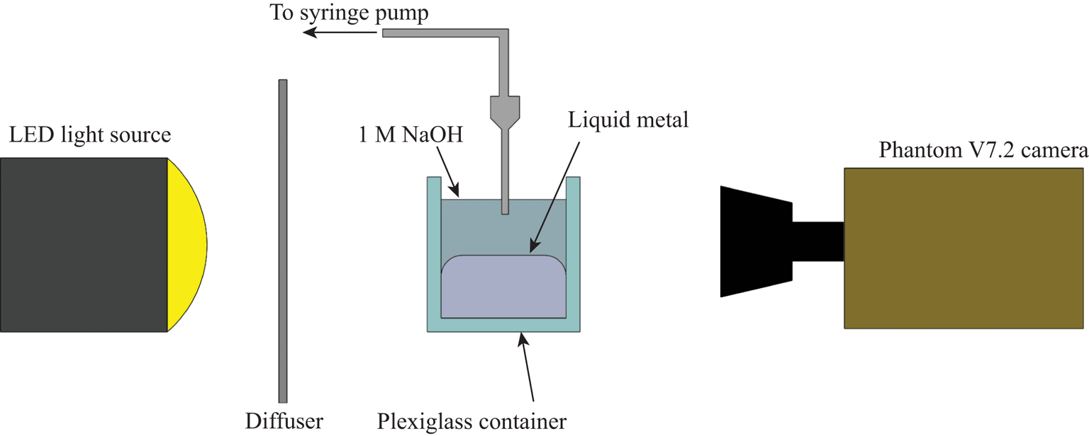
Figure 2. Experiment set-up.
The high speed camera was mounted to the table and levelled to the liquid interface. The resolution for video is  $640\times 480$ for all tests. The frame rate was somewhat limited as the cascade process can be quite long, of the order of whole seconds. The camera memory is finite so the frame rate must be balanced with the recording window in order to capture as much of the process as possible. The frame rate for all tests is between 5000 and 6024 frames per second. The spatial resolution is 0.014 px mm $^{-1}$ for all tests. The exposure time was kept constant at 98 $\mathrm {\mu }$s in order to ensure uniformity of lighting conditions for all tests. Note that figure 1 uses a separate set-up and is for demonstrative purposes only, the results do not include data from that particular set-up.
The NaOH used in every experiment was 1 M in concentration and was mixed in water. The density used is taken to be  $\rho _o =1040$ kg m $^{-1}$ and the viscosity is $\mu _o=1.3 \times 10^{-3}$ Pa s. The RTLM is composed of 68.5 % Ga, 21.5 % In and 10 % Sn, as mentioned above. The values we use in calculations match those in table 1 with the density and IFT verified prior to testing. The density was measured with a laboratory scale and found to match the expected value of 6440 kg m $^{-3}$. The IFT was measured with a KRÜSS Scientific Drop Shape Analyzer-DSA100. Using the pendant drop method the IFT was found to be in full agreement with the value reported in the table 1 of $\sigma = 0.404$ N m $^{-1}$.
The needle was actuated via a stepper motor to be as close to the interface as possible so as to minimize any inertial effects from the generation of the initial droplet. Additionally, the flow rate from the syringe pump was kept at 0.50  $\mathrm {\mu }$l s $^{-1}$. In order to prevent reaction with both the RTLM and the NaOH, polymer needles were used that were composed of either polytetrafluoroethylene or polypropylene depending on the needle size. A few sizes of needle were used ranging from 21G to 30G. For every drop produced we were able to observe and measure three to five partial coalescence events. Although the cascade continued further, the droplets were below the resolution of the camera.
Some consideration was needed in choosing the container as well. The container was a rectangular, Plexiglas prism and was placed so that one face was normal to the camera to prevent optical distortion. Due to the material cost, it was desirable to minimize the volume of liquid metal needed in the container. However, eliminating effects from the sidewalls and bottom panel were also important. For the bottom panel, the minimum fluid height needed to be above the so-called ‘shallow water’ condition which is defined as the case  $ky\rightarrow 0$ where $k$ is the wavenumber $k = 2 {\rm \pi}/ \lambda$, where $\lambda$ is the wavelength, and $y$ is the depth (De Gennes, Brochard-Wyart & Quéré Reference De Gennes, Brochard-Wyart and Quéré2013). The largest droplet had a diameter of 2.881 mm so taking this as the wavelength the was vector is $k = 2180$. This led to the choice of a depth of 22 mm which was gave a value of $ky = 48$ which we deemed sufficient to avoid shallow water effects. The capillary length provided an additional complication as the value for RTLM in NaOH is $l_c = 2.76$ mm. The reduced metal is highly non-wetting on the Plexiglas so the curvature at the walls was severe. If the container was not large enough the curvature would affect the free surface and the droplets would skate off on the lubrication layer between the two metal surfaces. Because of this a $38.1\ \textrm {mm}\times 38.1\ \textrm {mm}$ base contained was selected. This was found to produce a sufficiently flat surface to mitigate the issue of droplets skating out of frame or focus.
ImageJ software was used to perform all measurements with the needles serving as the physical reference scale. The droplets were then measured before and after each coalescence event for their diameter which was halved to give  $R_1$ and $R_2$. The bounce height $h$ was also measured with the undeformed free surface used as a reference for all height data. Time is measured by combining the frame number with the known frame rate creating a known time interval between frames, which was used to determine the coalescence time.
3. Mathematical model
For this study our primary focus is to develop a model for the dynamics of the droplet as it impacts the interface, rebounds and climbs to a maximum height while accounting for viscous effects. Secondarily, we will seek to confirm the velocity of the daughter droplet as given by (1.5) and assess the relative contributions of gravity and capillarity. This process is shown in more detail in figure 3 and defined schematically in figure 4. The first image of this figure represents the initial droplet of radius  $R_1$ residing on the free surface. The capillary wave then initiates and travels up the drop surface until a fluid column is formed at 6.4 ms in the figure. Capillary forces and gravity act on the mass of fluid that will become the daughter droplet and the image at 8.6 ms depicts the droplet immediately before pinch-off has occurred. The droplet then descends with initial velocity $V_0$ before impacting the surface, rebounding and reaching a maximum height $h_{max}$ as shown in the seventh image in the sequence at 31 ms. The droplet then descends to the interface and begins a new residence time. During this time the outer fluid is squeezed out slowly, and at 612.8 ms the capillary wave can be seen propagating again as the cascade continues. The smaller droplet is reassigned the role as father droplet for this new sequence and its radius becomes the new value of $R_1$.
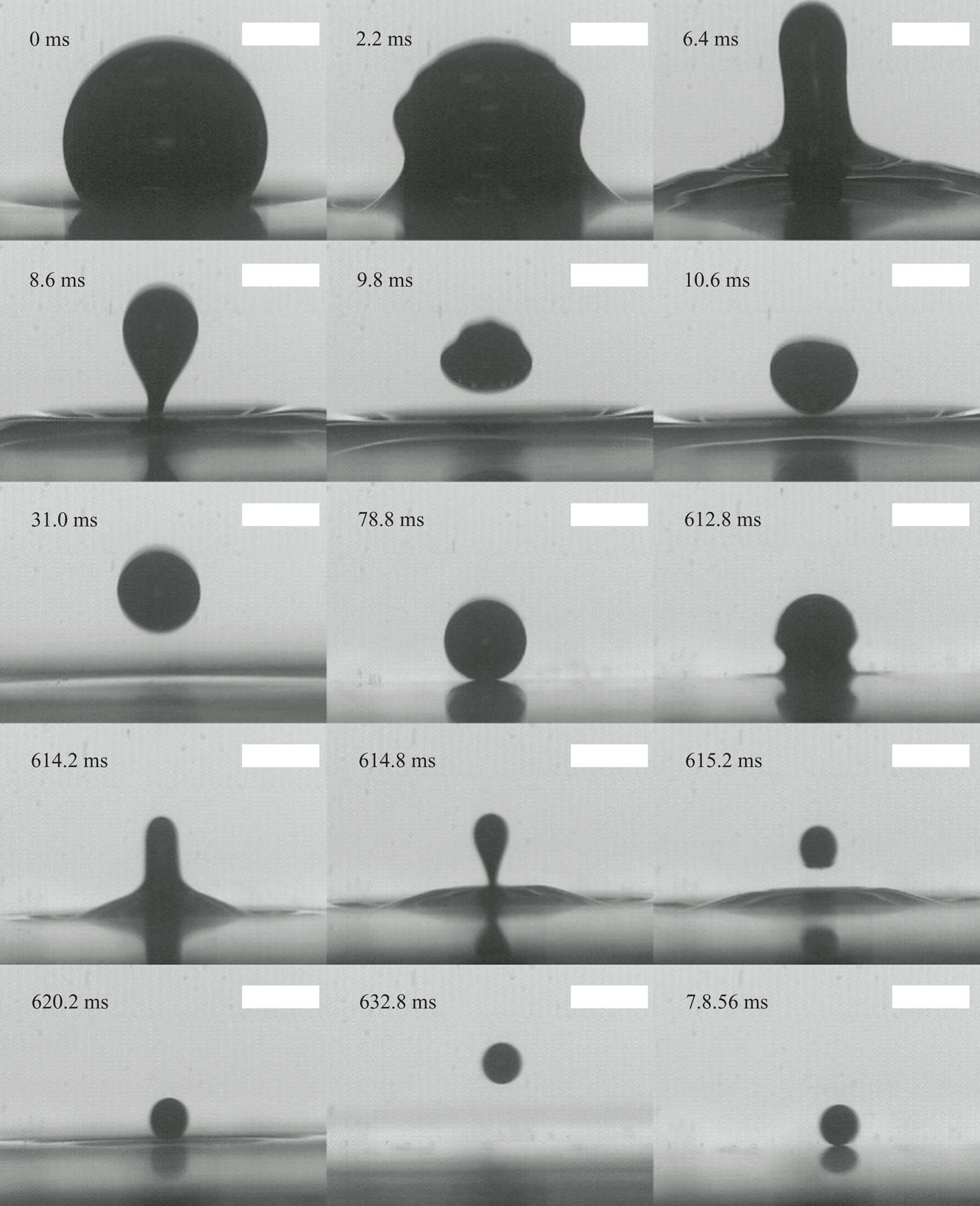
Figure 3. Partial coalescence sequence and bounce. Scale bars represent 1 mm.
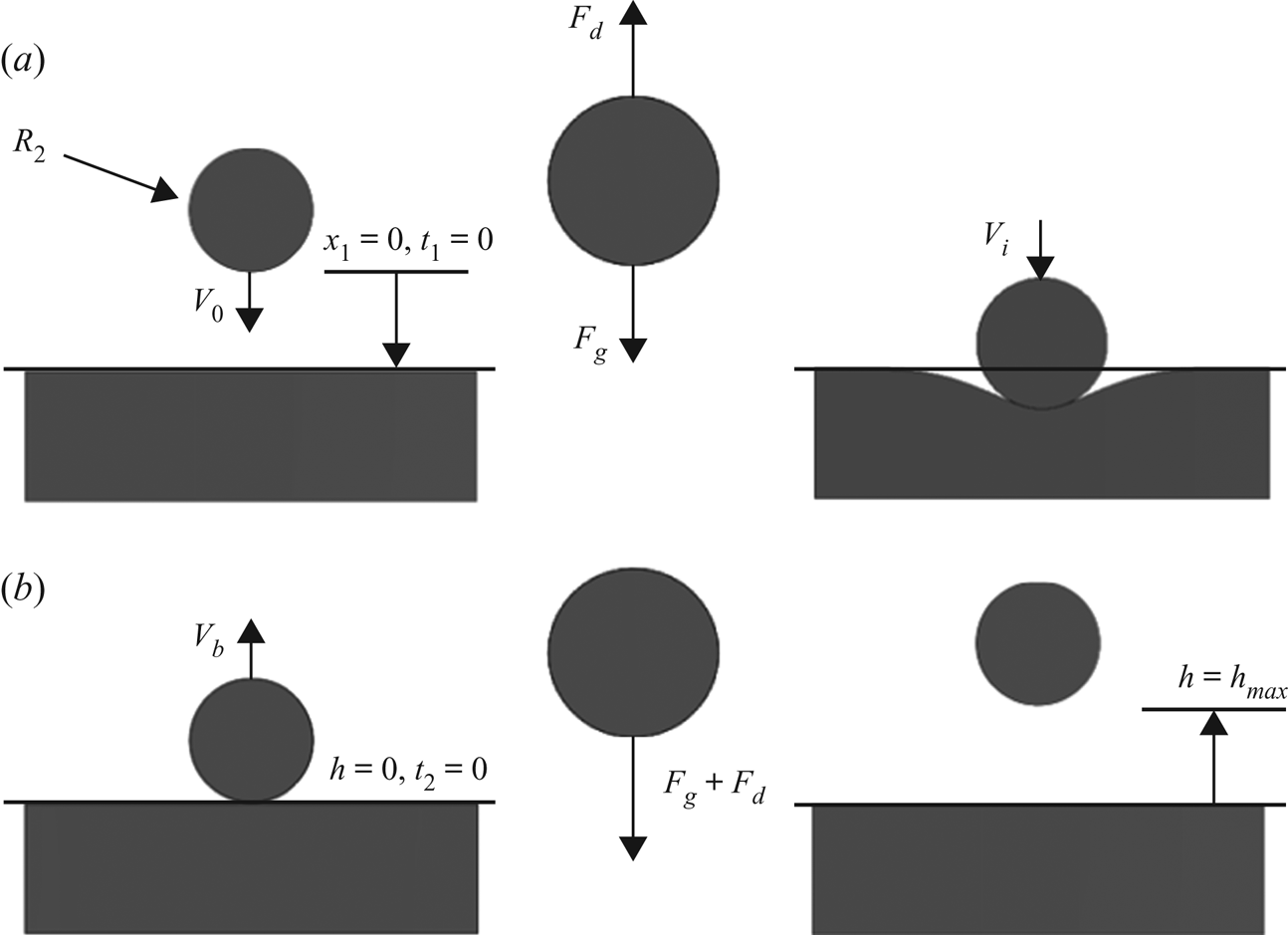
Figure 4. (a) Downward portion of bouncing droplet sequence. (b) Upward portion terminating in  $h_{max}$.
In order to analyse this phenomenon it is convenient to break the bouncing sequence into two parts: the downward portion and the upward portion. Figure 4(a) depicts the downward sequence. We will begin by using the famous model for creeping flow on a sphere as derived Stokes (Reference Stokes1851). This will require a modification to the effective viscosity since the inner droplet is a liquid and not a rigid sphere. An effective or net viscosity  $\mu _{net}$ can be found and is expressed as follows per White & Corfield (Reference White and Corfield2006):
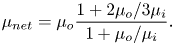 \begin{equation} \mu_{net} = \mu_o \frac{1+ 2 \mu_o / 3 \mu_i}{1 + \mu_o / \mu_i}. \end{equation}
 For the fluids used here (3.1) gives a value of  $0.880 \mu _o$ or $1.11\times 10^{-3}$ Pa s. The drag on a droplet can then be modelled as $F_d = F_{d,s} = 6 {\rm \pi}\mu _{net} R_2 V$. This allows us to write the equation of motion for the droplet undergoing gravity forces and Stokes’ drag
 \begin{equation} \rho \rlap{-}{V} \ddot{x}_1 = F_g - F_d = \Delta \rho \rlap{-}{V} g - 6 {\rm \pi}\mu_{net} R_2 \dot{x}_1. \end{equation}
 Here,  $\rlap{-}{V}$ is the volume of the droplet of radius $R_2$ and the variables $x_1$ and $t_1$ are the spatial and time systems for the downward portion. At $t_1 = 0$ the droplet is subject to the following initial conditions: $\dot {x}_1(0) = V_0$, $x_1(0) = 0$. The initial velocity $V_0$ is calculated via (1.5). Equation (3.2) can be readily integrated analytically to yield equations of motion for the droplet
 $$\begin{gather} x_1 = \beta ' g t_1 - \beta (\beta ' g - V_0) \left[1 - \exp \left(\frac{-t_1}{\beta} \right) \right], \end{gather}$$
 $$\begin{gather}\dot{x}_1 = \beta ' g - (\beta ' g - V_0) \exp \left(\frac{-t_1}{\beta} \right), \end{gather}$$
where
 \begin{equation} \beta = \frac{2\rho R_2^2}{9 \mu_{net}}, \quad \beta ' = \frac{2 \Delta \rho R_2^2}{9 \mu_{net}}. \end{equation}
 Equations (3.3)–(3.5a,b) are familiar equations associated with the stopping distance of small spheres at low Reynolds numbers. Specifically, we are looking for the conditions at which the droplet impacts the interface which is found by setting  $x_1 = 2 R_1 - 2 R_2 = 2 R_1 (1 - r_i)$, the initial height from the surface. Equation (3.3) is then solved numerically to find the impact time $t_1 = t_{impact}$. This time is plugged into (3.4) to find the velocity at impact such that $\dot {x}_1(t_{impact}) = V_i$, the velocity at impact. This impact velocity will provide the initial condition to calculate the bounce height. However, energy is not conserved in the impact with the interface. Jayaratne & Mason (Reference Jayaratne and Mason1964) studied the impact of droplets with a free surface. They modelled the impact as a simple harmonic and proposed a coefficient of restitution, $A$, which is defined as
 \begin{equation} A = \frac{V_b}{V_i}. \end{equation}
 Jayaratne and Mason found this value to be 0.22 for water droplets impacting a free surface, also comprised of water, which corresponds to a loss of 95 % of kinetic energy from the rebound. This gives a way to determine  $V_b$ which will provide the means to integrate the upward portion of the bounce as defined in figure 4(b). This portion uses a new coordinate and time scale to keep the calculation simple, as well as allowing us to neglect the time period associated with deforming the interface. In the figure $h = 0$ represents the plane of the undeformed free surface and $t_2$ is a new time variable that begins as the droplet leaves the surface. This results in a slightly different equation of motion that (3.2)
 \begin{equation} \rho \rlap{-}{V} \ddot{h} ={-} F_g - F_d ={-} \Delta \rho \rlap{-}{V} g - 6 {\rm \pi}\mu_{net} R_2 \dot{h}, \end{equation}
due to the fact that both drag and gravity now act against the direction of motion. Equation (3.7) can be analytically integrated and subjected to the initial conditions  $h(0) = 0$, $\dot {h}(0) = V_b$ to yield
 $$\begin{gather} h ={-} \beta ' g t_2 + \beta (\beta ' g + V_b) \left[1 - \exp\left(\frac{-t_2}{\beta} \right) \right], \end{gather}$$
 $$\begin{gather}\dot{h} ={-} \beta ' g + (\beta ' g + V_b) \exp \left( \frac{-t_2}{\beta} \right), \end{gather}$$
where  $\beta$, $\beta '$ are still given by (3.5a,b). The maximum height is found when $\dot {h}=0$ and occurs at time
 \begin{equation} t_{max} = \beta \ln{\left(\frac{V_b}{\beta ' g} +1 \right)}. \end{equation}
 Plugging this in to (3.8) yields an equation for  $h_{max}$
 \begin{align} h_{max} &={-} \beta ' g \left(\beta \ln{\left(\frac{A V_i}{\beta ' g} +1 \right)} \right) \nonumber\\ &\quad + \beta (\beta ' g + AV_i) \left[1 - \exp\left(\frac{ \left(-\beta \ln{\left(\dfrac{A V_i}{\beta ' g} +1 \right)} \right)}{\beta} \right) \right]. \end{align}
 Note that this equation has substituted  $V_b$ for $A V_i$ per (3.6). Equation (3.11) is convenient in that it is the result of analytical integration and provides a value $h_{max}$ that can readily be measured. However, this model is incomplete in that it is predicated on Stokes’ law which can only be faithfully applied up to Reynolds numbers $Re \ll 1$ where $Re = \rho _o V D / \mu _{net}$. This is insufficient for this system which may see Reynolds numbers above this threshold. While Stokes’ law may not be valid throughout the full sequence, it does provide the basis for a more precise solution.
Beard & Pruppacher (Reference Beard and Pruppacher1969) published empirically derived results for drag on droplets from the Stokes regime to  $Re = 200$. Later, Greene et al. (Reference Greene, Irvine, Gyves and Smith1993) were able to validate these results and extend the validity of the model to $Re \sim 1000$. The drag relationship is as follows:
 \begin{equation} \frac{F_d}{F_{d,s}} =
\left\{\begin{array}{@{}ll} 1+0.102 Re^{0.955}, & 0.2 \le Re
\le 2.0, \\ 1+0.115 Re^{0.802}, & 2.0 < Re \le 21.0, \\
1+0.189 Re^{0.632}, & 21.0 < Re \le 1000
\end{array} \right. \end{equation}
\begin{equation} \frac{F_d}{F_{d,s}} =
\left\{\begin{array}{@{}ll} 1+0.102 Re^{0.955}, & 0.2 \le Re
\le 2.0, \\ 1+0.115 Re^{0.802}, & 2.0 < Re \le 21.0, \\
1+0.189 Re^{0.632}, & 21.0 < Re \le 1000
\end{array} \right. \end{equation}
where  $F_d$ is the drag and $F_{d,s}$ is the Stokes drag. Equation (3.12) can be combined with the first parts of (3.2) and (3.7) to give a better estimate for the dynamics of the bouncing droplet. The weakness of this approach is that the equations become nonlinear and no longer can be integrated analytically. To account for this fact, the equations were integrated numerically using a fourth-order Runge–Kutta (RK4) scheme with step size $\textrm {dt}= 1\times 10^{-6}$ s. The solution procedure is similar to the Stokes procedure as detailed in figure 4. First, the equations are integrated until the stopping condition of $x_1 = 2 R_1 (1-r_i)$ is reached and the corresponding velocity at this time step is read and used to calculate the Reynolds number and apply the correct function from (3.12) for the subsequent time step. The coefficient of restitution was determined by comparing the measured height data with the upward portion and using the shooting method to solve for $A$. This was done separately from plotting $h_{max}$ which was done using the average value for the restitution coefficient from the data. The stop condition for integration on the upward portion is reached when the velocity was less than or equal to 0.
4. Results and analysis
The bounce height was calculated using the Stokes drag and (3.1)–3.11 and is plotted in figure 5(a). In the same figure the equations of motion were integrated using the Beard model and an RK4 scheme and plotted along with the measured experimental data. The behaviour of the model can be segmented into three distinct regions governed by gravity, capillarity, and viscous forces similar to the findings of Chen, Mandre & Feng (Reference Chen, Mandre and Feng2006). In this figure, the restitution coefficient  $A$ and the droplet ratio $r_i$ were held constant at $A = 0.27$ and $r_i = 0.47$ which were extracted from the data. Figure 5(b) depicts a hypothetical fluid system where in the inner fluid has the same fluid properties as the liquid metal but the net viscosity is varied over several orders of magnitude to demonstrate the importance of the viscosity of the quiescent fluid on the bouncing behaviour of the droplet. The inviscid case is equivalent to the model our group previously developed for modelling bouncing droplets in air (Honey & Kavehpour Reference Honey and Kavehpour2006) and is given by
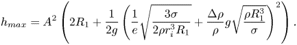 \begin{equation} h_{max} = A^2\left(2 R_1 + \frac{1}{2 g} \left( \frac{1}{e} \sqrt{\frac{3 \sigma}{2 \rho r_i^3 R_1}} +\frac{\Delta \rho }{\rho} g \sqrt{\frac{\rho R_1^3}{\sigma}} \right) ^2\right). \end{equation}
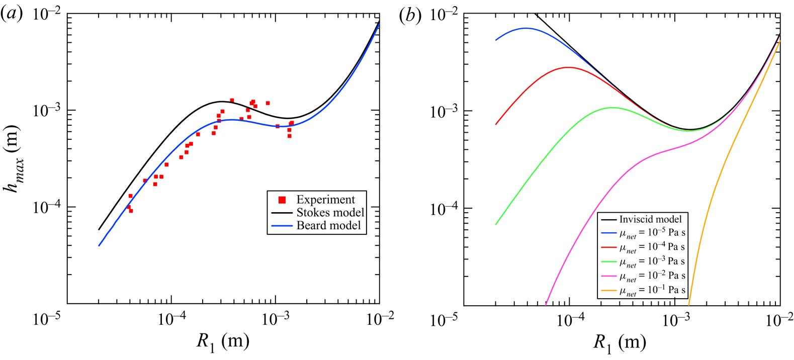
Figure 5. (a) Partial coalescence maximum bounce height  $h_{max}$ models for Beard and Stokes models of drag are included. For this plot $A = 0.27$ and $r_i = 0.47$. (b) Beard model plotted for various viscosities $\mu _{net}$. The black line indicates the inviscid case with viscosity increasing accordingly. The inviscid model was derived by Honey & Kavehpour (Reference Honey and Kavehpour2006) and is given by $h_{max} = A^2(2 R_1 + ({1}/{2g}) (({1}/{e}) \sqrt {{3 \sigma }/{(2 \rho r_i^3 R_1)}} +({\Delta \rho }/{\rho }) g \sqrt {{\rho R_1^3}/{\sigma }} ) ^2$.
Figure 5(a,b) is best interpreted reading the  $x$-axis from right to left as this as the direction in which the partial coalescence cascade occurs.
The first region in figure 5(a) exists for  $R_1 > 1.11$ mm which corresponds to a Bond number $Bo > 0.16$. This region can be considered the gravity dominant region. As droplets get too large the model loses usefulness as the droplets can no longer be approximated as spheres. It can be seen that in this region a larger droplet results in a greater bounce height, which can be interpreted as gravity affecting a higher initial velocity $V_0$ as the droplets become more massive. For the region where $Bo \le 0.16$ gravity effects begin to become unimportant and capillarity becomes the driving force for the droplet behaviour. In the inviscid case, depicted in black in figure 5(b), the droplet will bounce higher and higher in perpetuity until the drop fully coalesces. When a viscous quiescent fluid is introduced viscous forces begin to dominate when the droplet becomes sufficiently small. We call the region bounded by $0.38\ \textrm {mm}< R_1 \le 1.11\ \textrm {mm}$ the capillary region where the bounce height increases as the partial coalescence cascade leads to smaller and smaller droplets. It is not appropriate to characterize this regime by the Bond number as gravity is no longer as important as viscosity or capillarity so we bound it by the Ohnesorge number, choosing the net viscosity, $\mu _{net}$ and calling this specific version of the number $Oh_{net}$. This gives a region bounded by $4.62\times 10^{-4} \le Oh_{net} < 7.89\times 10^{-4}$. As shown in figure 5(b), the viscosity strongly governs the size of the capillary regime. At $\mu = 10^{-2}$ Pa s the capillary regime is barely apparent and at $\mu = 10^{-1}$ Pa s it is lost entirely, and the gravity and viscous regimes have no distinct division between them.
As the partial coalescence cascade continues past the final local maximum at  $R_1 = 0.38$ mm the bounce height only decreases as viscous forces dominate the motion of the droplet. This region is defined by $R_1 < 0.38$ mm or $Oh_{net} \ge 4.62\times 10^{-4}$. The Ohnesorge number is still quite small as the cascade proceeds into the viscous region. Assuming that the partial coalescence will proceed as $Oh \xrightarrow {} 1^-$ as seen in our previous, inviscid, experiments (Aryafar & Kavehpour Reference Aryafar and Kavehpour2006), the partial coalescence cascade would proceed until the droplet radius was $1$ nm. However, per the model, the bounce height decreases faster than the radius of the droplet and at $R_1 = 900$ nm the bounce height is only $h_{max} = 90$ nm, an order of magnitude lower, so any noticeable bouncing would cease as the droplet radius approaches the $\sim$1 $\mathrm {\mu }$m scale. Unfortunately, the cascade was observed to continue past the reported values, but the resolution of the camera was insufficient to capture the droplets. Observing this cascade into the micro and possibly nano scales will be the subject of future research.
The relative performance of the Beard and Stokes drag models can be readily compared in figure 5(a) as well. Both models agree in the gravity region, which is expected as gravity body forces dominate viscous forces, as this is the facet of the models that is unchanged between them. The Beard model then performs much better in the capillary region near the local minimum as well as in the viscous region. The local maximum separating the viscous and capillary regions is shifted to the right in the numerical model as compared with the Stokes model as well and more closely matches the data. This is due to the fact that the Stokes model under-predicts the magnitude of drag in regions where the Reynolds number is near or above unity. The Stokes model does perform slightly better in the mid capillary region which is surprising and warrants further investigation.
Figure 6(a) depicts the restitution coefficient as a function of the dimensionless radius  $R_1^*$, where $R_1^*$ is the radius divided by the capillary length $R_1^* = R_1/\sqrt {\sigma / \Delta \rho g}$. For these individual values the restitution coefficient was found using the shooting method, with the $h_{max}$ from the data serving as the corresponding boundary value. The value for the RTLM was found to be $A = 0.27 \pm 0.06$. While this value is higher than the value of $A = 0.22$ as measured by Jayaratne and Mason, it does fit with the data from our previous work published which found values of $A_{meth} = 0.21 \pm 0.08$, $A_{water} = 0.27 \pm 0.01$, $A_{SiOil} = 0.27 \pm 0.03$ for methanol, water and silicone oil, respectively. This restitution coefficient corresponds to a 93 % loss of kinetic energy as opposed to the 95 % loss noted previously. This could be due to improvements in measurement equipment, or to the fact that Jayaratne and Mason were limited to studying droplet impacts at oblique angles and estimating the coefficient for normal impacts which we were able to observe directly. While the values of $A$ were generally slightly higher for larger values of $R_1^*$, the difference was not significant and no part of the theory predicts a function of droplet size affecting the bounce velocity ratio.
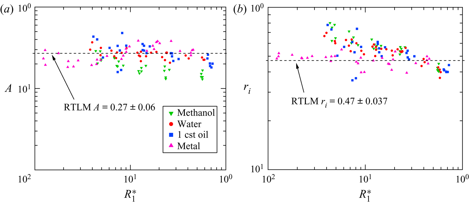
Figure 6. (a) The restitution coefficient  $A$ vs the normalized radius $R_1^*$. (b) The droplet ratio $r_i$ vs the normalized radius $R_1^*$. In both instances the droplet radius is normalized by the capillary length $R_1^* = R_1/\sqrt {\sigma / \Delta \rho g}$. Supplementary data are sourced from experiments published previously (Honey & Kavehpour Reference Honey and Kavehpour2006).
Figure 6(b) depicts the drop ratio coefficient as a function of dimensionless radius  $R_1^*$. The mean value was found to be $r_i = 0.47 \pm 0.037$ which is in good agreement with the remaining data plotted which include $r_{i,meth} = 0.65 \pm 0.08$, $r_{i,water} = 0.58 \pm 0.06$, $r_{i,SiOil} = 0.52 \pm 0.05$ for methanol, water and silicone oil, respectively. The droplet ratio for RTLM was lower than the other three liquids but performed fairly similarly to silicone oil.
Of additional interest to this study is further investigation of (1.5), the initial downward velocity of the daughter droplet of radius  $R_2$. By inspection, the equation has two parts: one gravitational term and one capillary term. To understand the relative contributions of each force we model the kinetic energy of the droplet with each contributing force applied in the absence of the other, in other words a pure capillary driven droplet vs a pure gravity driven droplet
 \begin{equation} E_{cap} = \frac{1}{2} \rho \left(\frac{1}{e} \sqrt{\frac{3 \sigma}{2 \rho r_i^3 R_1}} \right)^2, \quad E_{grav} = \frac{1}{2 \rho} \left(\Delta \rho g \sqrt{\frac{\rho R_1^3}{\sigma}} \right)^2, \end{equation}
and the total kinetic energy is found from the entirety of (1.5) to give
 \begin{equation} E_{tot} = \frac{1}{2} \rho \left( \frac{1}{e} \sqrt{\frac{3 \sigma}{2 \rho r_i^3 R_1}} +\frac{\Delta \rho }{\rho} g \sqrt{\frac{\rho R_1^3}{\sigma}} \right)^2. \end{equation}
 By dividing (4.2) by (4.3) the relative contributions are found and plotted vs  $R_1$ in figure 7(a). The intersection of these two is $3.27$ mm, which would make for a very large droplet, larger than any produced in this work. This indicates that the capillarity serves as the primary driver of the partial coalescence bouncing phenomenon. This explains why the bouncing is usually observed in air and not in a quiescent viscous fluid, the surface tension simply is not high enough to generate a sufficient initial velocity to overcome viscous resistance. The RTLM has very high interfacial tension, a full order of magnitude higher than most non-metallic liquids, which provides the needed kinetic energy to bounce.
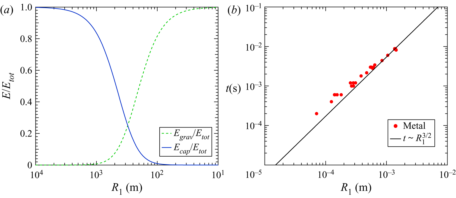
Figure 7. (a) Ratio of energy contributions of capillary forces and gravity forces to overall daughter droplet downward kinetic energy  $E/E_{tot}$. (b) Coalescence time vs droplet diameter. Plotted against a power law function corresponding to $t \sim R_1^{3/2}$.
Figure 7(b) shows the coalescence time plotted against the initial droplet radius. Thoroddsen & Takehara (Reference Thoroddsen and Takehara2000) predicted this was governed by the capillary time  $t_cap$. In fact, when the coalescence time data are plotted and fitted with a power law fit the data match very well, affirming the result from Thoroddsen and Takehara as well as other prior work that related the capillary time to the coalescence time. As $Oh \xrightarrow {} 1^-$ the viscous time scale is expected to begin to govern the coalescence behaviour but this was not observed due to the low Ohnesorge numbers present in this work. Residence time was also noted for the droplets, however, there was no discernible pattern to the duration between coalescence events indicating a high degree of nonlinearity in the residence period before the onset of the subsequent coalescence event.
As a final note the value of  ${\rm \pi} / Z_0$, the ratio of the circumference over the wavelength, was calculated per (1.1) for all partial coalescence events. The Tomotika model predicts a value ${\rm \pi} / Z_0 = 0.548$ but the value from this work was found to be ${\rm \pi} / Z_0 = 0.840 \pm 0.10$. Previous work reached similar conclusions about Tomotika's model (Charles & Mason Reference Charles and Mason1960b; Aryafar & Kavehpour Reference Aryafar and Kavehpour2006). Taken together this information indicates that the viscosity ratio is likely not the best predictor of the normalized wavelength for partial coalescence.
5. Conclusion
In this manuscript we performed drop–planar partial coalescence experiments that resulted in droplets bouncing on the interface of RTLM alloy with 1 M sodium hydroxide as a quiescent fluid. These resulted in a range of drop sizes from  $0.039\ \textrm {mm} \le D_1 \le 1.440\ \textrm {mm}$. We first employed Stokes’ law to develop a first-order model for viscous effects on the droplet. This model was improved upon with a numerical model to simulate the dynamics of a bouncing droplet by applying the drag force as attained by Beard & Pruppacher (Reference Beard and Pruppacher1969) and integrating the equations of motion over the downward and then subsequent upward trajectory of the drop. We also further validated the model for droplet initial velocity first proposed by Aryafar & Kavehpour (Reference Aryafar and Kavehpour2006) and demonstrated the importance of the capillary force in creating the conditions for droplet bouncing to occur. In doing so we were able to identify three distinct regions for the bouncing phenomena. The first region is bound by $Bo > 0.16$ and is known as the gravity dominant region. The second is bound by the conditions $Bo \le 0.16$ as well as $4.62\times 10^{-4} \le Oh_{net} < 7.89\times 10^{-4}$, where $Oh_{net}$ is the Ohnesorge number with the combined viscosity per (3.1) serving as the viscosity term. This region is known as the capillary region as it is dominated by interfacial forces. The third region is given by $Oh_{net} <4.62\times 10^{-4}$ and is known as the viscous region as the droplet's behaviour is dominated by viscous forces. The restitution coefficient as defined by Jayaratne & Mason (Reference Jayaratne and Mason1964) was also determined numerically via the shooting method and found to be $A = 0.27 \pm 0.06$ a result that is in line with previous research (Honey & Kavehpour Reference Honey and Kavehpour2006). The droplet ratio was found to be $r_i = 0.47 \pm 0.037$ a result that is slightly low compared with other substances with similar Ohnesorge numbers. The coalescence time was also compared with existing theory that finds $t_c \sim R^{3/2}$ which conforms to existing theory posed by Thoroddsen & Takehara (Reference Thoroddsen and Takehara2000). We would expect this to change as the drops got smaller and $Oh \rightarrow {1^-}$. Finally, we tested the ratio of the droplet circumference to the wavelength ${\rm \pi} /Z_0$ vs the theory posed by Tomotika (Reference Tomotika1935) and found a value of ${\rm \pi} / Z_0 = 0.840 \pm 0.10$ vs the predicted value of 0.548, further affirming that the viscosity ratio is not sufficient to model the droplet breakup wavelength. Taking this all together we have built upon the inviscid model for a bouncing droplet and extended it to apply to a viscous quiescent fluid in cases where the IFT is high enough to result in bouncing.
Funding
This work was funded in part by the U.S. Navy NEEC program grant award Number N00174-17-1-0004.
Declaration of Interests
The authors report no conflicts of interest.


 Open access