


1. Introduction
Droplet spreading alongside mass transfer through interfacial phase change is a moving boundary problem that involves the interaction of liquid and air with an impermeable solid substrate. As a fundamental problem in fluid mechanics, droplet spreading exemplifies the general problem of a moving contact line, which covers a lot of common phenomena in our daily life and in industrial applications. In past decades, researchers have developed a series of mathematical models for explicitly understanding the droplet dynamics during this process.
In this research, we focus on the behaviours of one type of hygroscopic ionic solution droplets with interfacial phase change. This kind of ionic solution, e.g. LiBr–H2O and LiCl–H2O, exhibits the ability to absorb water vapour due to the adhesion of hygroscopic ions to water molecules, and has been widely applied in innovative dehumidification (Liu, Jiang & Qu Reference Liu, Jiang and Qu2007; Wang, Zhang & Li Reference Wang, Zhang and Li2017) and water-harvesting systems (Wang, Zhang & Li Reference Wang, Zhang and Li2016; Ahmed et al. Reference Ahmed, Gandhidasan, Zubair and Bahaidarah2017). Depending on the humidity of the ambient air, evaporation or vapour absorption takes place, and the salt concentration within the droplet changes. The variation of salt concentration changes the vapour pressure difference between the droplet surface and the surrounding air, which in turn affects the interfacial mass flux (Wang et al. Reference Wang, Orejon, Sefiane and Takata2019a) and the droplet dynamics.
Besides the difficulties shared by most moving boundary problems, the simulation of droplets with a moving contact line presents additional complications (de Gennes Reference de Gennes1985; Bonn et al. Reference Bonn, Eggers, Indekeu, Meunier and Rolley2009). At the liquid–solid interface, there is an inherent contradiction in simultaneously assuming the no-slip boundary condition and expecting a displacement between liquid and gas there; therefore, a force singularity will arise at the moving contact line (Huh & Scriven Reference Huh and Scriven1971; Dussan & Davis Reference Dussan and Davis1974; Dussan Reference Dussan1979). Greenspan (Reference Greenspan1978) developed a model for the movement of a small viscous droplet on a surface based on the lubrication equations and applied the dynamic contact angle to describe the forces acting on the fluid at the contact line. Ehrhard & Davis (Reference Ehrhard and Davis1991) further developed Greenspan's model by taking account of the effects of gravitational force and thermocapillary force, and generalized the relationship between the advancing contact angle and the speed of the contact line based on the empirical correlations derived by previous researchers (e.g. Tanner Reference Tanner1979; Cazabat & Stuart Reference Cazabat and Stuart1986; Chen & Wada Reference Chen and Wada1989).
Subsequently, Haley & Miksis (Reference Haley and Miksis1991) developed a lubrication model for droplet spreading, which includes the effect of liquid slip on solid substrates, and relates the dynamic contact angle with the velocity of the contact line. This approach, though, relies on the use of reliable functions between the dynamic contact angle and the contact line motion. The problem has been addressed later to some extent by a number of experimental studies (Ehrhard Reference Ehrhard1993; Sedev et al. Reference Sedev, Budziak, Petrov and Neumann1993; Eggers & Stone Reference Eggers and Stone2004; Blake Reference Blake2006). Anderson & Davis (Reference Anderson and Davis1995) also took account of the effect of evaporation and developed a one-sided model to describe the dynamics of a two-dimensional volatile liquid droplet on a uniformly heated plate. A similar contact line model, albeit solving the full two-dimensional problem, was used by Karapetsas et al. (Reference Karapetsas, Matar, Valluri and Sefiane2012) to predict the formation of travelling hydrothermal waves, arising from the temperature gradient as a result of natural evaporation, reported in previous experimental work (Sefiane et al. Reference Sefiane, Moffat, Matar and Craster2008).
More recently, a similar explicit contact line model has been utilized to model the spreading of more complex systems such as a surfactant-laden droplet spreading over solid or liquid substrates (Karapetsas, Craster & Matar Reference Karapetsas, Craster and Matar2011a,Reference Karapetsas, Craster and Matarb) and thermocapillary-driven migration of thin droplets (Karapetsas, Sahu & Matar Reference Karapetsas, Sahu and Matar2013; Karapetsas et al. Reference Karapetsas, Sahu, Sefiane and Matar2014). A different, less popular, approach that has been suggested in the literature is to connect the macroscopic droplet bulk with the extending solid surface through a microscopic structure (Shikhmurzaev Reference Shikhmurzaev1997), referred to as the interface formation model in later studies (Sibley, Savva & Kalliadasis Reference Sibley, Savva and Kalliadasis2012; Snoeijer & Andreotti Reference Snoeijer and Andreotti2013). The microscopic contact angle, as part of the solution, is determined according to the contact line conditions arising from a local mechanical balance with no assumptions required on its velocity dependence from the experimental results. The interface formation model is more complex compared to the former approach and is still subject to debates on its physical basis, while the exploration of the microscopic physics, e.g. rolling or not, is effort-worthy and closest to a comprehensive mathematical description.
Another popular approach, as adopted in this research, is based on the assumption of a precursor film adsorbed at the gas–solid surface in front of the three-phase contact line (TPCL) (de Gennes Reference de Gennes1985). The precursor film is a result of the long-range intermolecular interactions, in the range of a few hundred molecules, and has been verified experimentally with the techniques of interference microscopy (Kavehpour, Ovryn & McKinley Reference Kavehpour, Ovryn and McKinley2003), fluorescence microscopy (Hoang & Kavehpour Reference Hoang and Kavehpour2011) and atomic force microscopy (Xu et al. Reference Xu, Shirvanyants, Beers, Matyjaszewski, Rubinstein and Sheiko2004), amongst others. Owing to the existence of precursor film, a smooth transition from the apparent contact angle to the flat solid surface is realized, thus avoiding the shear stress singularity. As reported in the review by Bonn et al. (Reference Bonn, Eggers, Indekeu, Meunier and Rolley2009), this approach has been utilized extensively to model perfectly wetting fluids, but it has also been successfully applied to model cases with partial wetting (see e.g. Schwartz Reference Schwartz1998; Schwartz & Eley Reference Schwartz and Eley1998; Gomba & Homsy Reference Gomba and Homsy2010) by introducing the effect of a non-zero contact angle through a disjoining–conjoining pressure term.
To account for the effect of evaporation, Ajaev (Reference Ajaev2005), following a similar approach, proposed a model based on the previous work of Moosman & Homsy (Reference Moosman and Homsy1980). Instead of applying the correlations between droplet contact angle and the contact line motion, Ajaev's model assumed a microscopic adsorbed film in the dry area on the heated surface, and that the adsorbed film is in thermodynamic equilibrium with both the vapour and solid phases. Owing to the van der Waals effect, equilibrium can be achieved by non-zero film thickness, thus avoiding the singularity at the contact line. In recent years, the latter approach has been further developed to simulate the spreading and evaporation phenomena of more complex droplets, such as those with nanoparticles (Matar, Craster & Sefiane Reference Matar, Craster and Sefiane2007; Craster, Matar & Sefiane Reference Craster, Matar and Sefiane2009), with colloidal suspensions (Maki & Kumar Reference Maki and Kumar2011), as well as in the study of particle deposition in the presence of surfactants (Karapetsas, Sahu & Matar Reference Karapetsas, Sahu and Matar2016), and the evaporation of droplets consisting of binary mixtures (e.g. ethanol–water) (Williams et al. Reference Williams, Karapetsas, Mamalis, Sefiane, Matar and Valluri2021). Besides the development of lubrication-type models for droplets with complex components, researchers have also developed models to simulate the observed interfacial phenomena and the droplet motion under external forces (Espín & Kumar Reference Espín and Kumar2014).
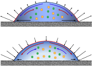
In recent years, studies on multicomponent droplets have revealed attractive physical phenomena (Lohse & Zhang Reference Lohse and Zhang2020) induced by the preferential evaporation of individual components or mediated by external vapour sources, e.g. the occurrence of density-driven flows (Edwards et al. Reference Edwards, Atkinson, Cheung, Liang, Fairhurst and Ouali2018; Li et al. Reference Li, Diddens, Lv, Wijshoff, Versluis and Lohse2019), phase segregation/separation (Li et al. Reference Li, Lv, Diddens, Tan, Wijshoff, Versluis and Lohse2018; Li et al. Reference Li, Diddens, Segers, Wijshoff, Versluis and Lohse2020; Mao et al. Reference Mao, Chakraverti-Wuerthwein, Gaudio and Kosmrlj2020), the transient Marangoni flow and solutal effects (Christy, Hamamoto & Sefiane Reference Christy, Hamamoto and Sefiane2011), etc. Specifically, in an evaporating multicomponent droplet, the spatiotemporal variation of interfacial mass flux induces the gradients of liquid density, temperature and concentration. The different physical processes interact with each other, induce varying flow patterns with phase transitions, and lead to various droplet dynamics and attraction–repulsion chasing behaviours of neighbouring droplets in specific cases (Cira, Benusiglio & Prakash Reference Cira, Benusiglio and Prakash2015). Owing to the complex coupling of these physical processes, numerical models of the evaporation of multicomponent droplets, to our knowledge, are rather limited. The few acknowledged approaches include numerical models using the lubrication assumption (Diddens et al. Reference Diddens, Kuerten, van der Geld and Wijshoff2017) and a finite element method with self-adapting mesh (Diddens Reference Diddens2017), which simulate the evaporation of binary volatile droplets and ouzo droplets (ternary mixture of a strongly hydrophobic essential oil, water and alcohol). Other trials also include the numerical modelling of aqueous NaCl solution droplets with commercial computational fluid dynamics software constrained to pinned droplets (Kang et al. Reference Kang, Lim, Lee and Lee2013; Pradhan & Panigrahi Reference Pradhan and Panigrahi2017).
The aim of this work is to develop a detailed mathematical model with the help of supporting experiments to fully reveal the behaviours of hygroscopic ionic solution droplets with both evaporative and absorptive mass fluxes. Here, the model is developed based on the lubrication theory, which fully accounts for the thermophysical properties of the ionic solution and the state of the surrounding environment. The model allows for the free motion of the TPCL by assuming a precursor film adsorbed at the solid substrate. An expression for the interfacial mass flux is derived by combining the Hertz–Knudsen equation with the fundamental thermodynamic equilibrium relationship across the liquid–air interface. Detailed experiments are subsequently carried out, which indicate a qualitative agreement with the numerical prediction.
In the following sections, the physical description and a detailed introduction to the mathematical model are presented in § 2. In § 3, we outline the boundary conditions, the initial conditions and the numerical method. Details of the fluid properties and the numerical approaches are provided in the appendix. The numerical results and discussions are then presented in § 4, including the evaporation of pure water droplets, the evaporation and vapour absorption of hygroscopic solution droplets, followed by a qualitative comparison with the experimental results. The concluding remarks and research perspective are summarized in § 5.
2. Problem formulation
We take a lithium bromide aqueous solution (LiBr–H2O) droplet as an example. Owing to the high adhesion force of Li+ ions and Br− ions to water molecules, the water vapour pressure at the droplet surface is greatly reduced. Depending on the ambient condition, the LiBr–H2O droplet either evaporates (at low ambient humidity) or absorbs water vapour (at high ambient humidity). Preferential evaporation/absorption induces concentration gradients, while the thermal effect along with water-vapour phase change induces temperature variation within the droplet (Wang et al. Reference Wang, Orejon, Sefiane and Takata2020).
The mass transfer process can be divided into vapour diffusion on the air side, water–vapour/vapour–water phase change at the interface, and solute diffusion within the droplet. Compared to the liquid phase, the density, viscosity and thermal conductivity of the gas phase are significantly smaller and can be neglected, namely,  ${\hat{\rho }_v} \ll {\hat{\rho }_l}$, ${\hat{\mu }_v} \ll {\hat{\mu }_l}$ and ${\hat{k}_v} \ll {\hat{k}_l}$. Moreover, the mass diffusion rate in the gas phase is 103–104 times that in the liquid phase $({D_{water/air}}/{D_{\textrm{LiBr}/\textrm{LiBr} - {\textrm{H}_2}\textrm{O}}}\sim {10^{ - 5}}/{10^{ - 9}}\sim {10^4})$ (Cussler Reference Cussler2009). Therefore, the concentration field of water vapour can be assumed to be homogeneous. Considering the characteristics of ionic solution droplets, we reasonably apply a one-sided model, which focuses on the physical processes within the ionic solution droplets. Compared to the two-sided model (Sáenz et al. Reference Sáenz, Sefiane, Kim, Matar and Valluri2015) and 1.5-sided model (Hu & Larson Reference Hu and Larson2002; Diddens et al. Reference Diddens, Kuerten, van der Geld and Wijshoff2017), the one-sided model is able to capture the main physical mechanisms in an efficient way, while maintaining a modest computational cost. Additionally, the model closely relates the interfacial mass flux with the ambient condition, and is able to capture the influence of ambient temperature and humidity.
2.1. Governing equations
Shown in figure 1, we consider a thin droplet with aspect ratio  $\varepsilon = {\hat{H}_0}/{\hat{R}_0} \ll 1$. The aqueous solution is considered as a Newtonian fluid and assumed incompressible. The thermal properties of LiBr–H2O solution are approximated as a function of the solution temperature and solute concentration (see appendix A). To remove the stress singularity arising from the moving contact line, a precursor film is assumed to exist at the solid surface in front of the TPCL. The precursor film is sufficiently thin so that the adsorption of water molecules onto the substrate is enhanced by van der Waals interactions. Owing to the extremely small thickness, the precursor film gets saturated and reaches environmental equilibrium very quickly upon contact with the humid air.

Figure 1. A sessile lithium bromide–water (LiBr–H2O) droplet in contact with humid air (mixture of dry air and water vapour):  ${\hat{H}_0}/{\hat{R}_0} \ll 1$ is assumed, ${x_{w,l}}(\hat{z},\hat{r},\theta ,\hat{\tau })$ refers to the concentration of water inside the droplet, xw,s refers to the concentration of water at the droplet interface, ${c_{{\textrm{H}_2}\textrm{O},I}}$ refers to the water vapour concentration in the humid air layer near the droplet interface, ${c_{{\textrm{H}_2}\textrm{O},\infty }}$ refers to the water vapour concentration in the air bulk (and is assumed as constant), and $\boldsymbol{n}$ and $\boldsymbol{t}$ denote the outward unit vectors acting in normal and tangential directions to the interface, respectively. The centre of the droplet base in contact with the substrate, O, is defined as the origin of the coordinates. A thin precursor film is assumed to exist on the solid surface in front of the TPCL.
A cylindrical coordinate system,  $(\hat{r},\theta ,\; \hat{z})$, is applied to solve the velocity field, $\hat{\boldsymbol{u}} = (\hat{u},\hat{v},\hat{w})$, where $\hat{u}$, $\hat{v}$ and $\hat{w}$ correspond to the horizontal, azimuthal and vertical components of the velocity field, respectively. The liquid–vapour interface is located at $\hat{z} = \hat{h}(\hat{r},\hat{t})$, while the liquid–solid and solid–vapour interfaces are located at $\hat{z} = 0$. The liquid phase is governed by the following incompressible mass, momentum, energy and concentration equations:
 \begin{gather}\hat{\boldsymbol{\nabla}}\boldsymbol{\cdot }\hat{\boldsymbol{u}} = 0,\end{gather}
 \begin{gather}\hat{\rho }\left( {\frac{{\partial \hat{\boldsymbol{u}}}}{{\partial \hat{t}}} + \hat{\boldsymbol{u}}\boldsymbol{\cdot }\hat{\boldsymbol{\nabla}}\hat{\boldsymbol{u}}} \right) = \hat{\boldsymbol{\nabla}}\boldsymbol{\cdot }\hat{\boldsymbol{\mathsf{E}}} + \hat{\rho }{\hat{\boldsymbol{g}}_G}, \end{gather}
 \begin{gather}\hat{\rho }{\hat{c}_p}\left( {\frac{{\partial \hat{T}}}{{\partial \hat{t}}} + \hat{\boldsymbol{u}}\boldsymbol{\cdot }\hat{\boldsymbol{\nabla}}\hat{T}} \right) = \hat{\boldsymbol{\nabla}}\boldsymbol{\cdot }(\hat{k}\hat{\boldsymbol{\nabla}}\hat{T}),\end{gather}
 \begin{gather}\frac{{\partial {\chi _{{\textrm{H}_2}\textrm{O}}}}}{{\partial \hat{t}}} + \hat{\boldsymbol{u}}\boldsymbol{\cdot }\hat{\boldsymbol{\nabla}}{\chi _{{\textrm{H}_2}\textrm{O}}} = \hat{\boldsymbol{\nabla}}\boldsymbol{\cdot }({\hat{D}_{{\textrm{H}_2}\textrm{O}}}\hat{\boldsymbol{\nabla}}{\chi _{{\textrm{H}_2}\textrm{O}}}).\end{gather}
Here  ${\hat{D}_{{\textrm{H}_2}\textrm{O}}}$ denotes the mass diffusion coefficient of water molecules, ${\hat{\chi }_{{\textrm{H}_2}\textrm{O}}}$ denotes the water concentration in LiBr–H2O solution, and $\hat{\boldsymbol{\mathsf{E}}}$ refers to the total stress tensor at the liquid side, defined as
 \begin{equation}\hat{\boldsymbol{\mathsf{E}}} ={-} \hat{p}\boldsymbol{\mathsf{I}} + \hat{\mu }(\hat{\boldsymbol{\nabla}}\hat{\boldsymbol{u}} + \hat{\boldsymbol{\nabla}}{\hat{\boldsymbol{u}}^\textrm{T}}),\end{equation}
where  $\boldsymbol{\mathsf{I}}$ denotes the identity tensor.
Along the droplet interface, the boundary equation of mass balance can be expressed by the relationship between the velocity of the liquid solution,  ${\hat{\boldsymbol{u}}}$, and the velocity of the interface, ${\hat{\boldsymbol{u}}_s}$,
 \begin{equation}(\hat{\boldsymbol{u}} - {\hat{\boldsymbol{u}}_s})\boldsymbol{\cdot }\boldsymbol{n} = \frac{{\skew4\hat{J}}}{{\hat{\rho }}},\end{equation}
where  $\skew4\hat{J}$ denotes the interfacial mass flux of water vapour and $\hat{\rho }$ denotes the density of the solution near the droplet interface. The jump energy balance can then be derived by taking account of the heat release at the liquid–vapour interface, expressed as
 \begin{equation}\skew4\hat{J}{\hat{L}_{{\textrm{H}_2}\textrm{O}}} + \hat{k}\hat{\boldsymbol{\nabla}}\hat{T}\boldsymbol{\cdot }\boldsymbol{n} = {\hat{k}_g}\hat{\boldsymbol{\nabla}}{\hat{T}_g}\boldsymbol{\cdot }\boldsymbol{n},\end{equation}
where  ${\hat{\rho }_g}$, ${\hat{\boldsymbol{u}}_g}$, ${\hat{k}_g}$ and ${\hat{T}_g}$ refer to the density, velocity, thermal conductivity and temperature of the gas phase, respectively, and ${\hat{L}_{{\textrm{H}_2}\textrm{O}}}$ denotes the latent heat of vaporization or the heat of absorption.
At the droplet surface, the transition of vapour molecules from liquid to gas phase will generate an inward normal force, namely the vapour recoil effect, which has been evidenced to be a destabilizing factor of interface dynamics (Burelbach, Bankoff & Davis Reference Burelbach, Bankoff and Davis1988). Nevertheless, the recoil force is practically only important for applications where very high mass fluxes are involved (Gad-el-Hak Reference Gad-el-Hak2005). In this study, evaporation or vapour absorption is driven by a vapour pressure difference of the order of several kilopascals. Therefore, the inward or outward pressure exerted by vapour recoil is relatively weak and resisted by the capillary and Marangoni effects. By ignoring the effect of vapour recoil and inertia from the gas phase  $({\hat{\mu }_v} \ll {\hat{\mu }_l})$, a relation between the normal stress jump, the surface tension, the mean curvature and the van der Waals interactions can be derived, namely, the normal stress boundary balance:
 \begin{equation}{-}\hat{p} + \boldsymbol{n}\boldsymbol{\cdot }\hat{\boldsymbol{\tau }}\boldsymbol{\cdot }\boldsymbol{n} = 2\hat{\kappa }\hat{\sigma } + \hat{\varPi } - {\hat{p}_g}.\end{equation}
Here  $\hat{p}$ is the pressure of the liquid phase, ${\hat{p}_g}$ is the total pressure of the gas phase, $\boldsymbol{\hat{\tau}}$ is the shear stress tensor of the liquid phase, $2\hat{\kappa } ={-} {\hat{\boldsymbol{\nabla}}_s}\boldsymbol{\cdot }\boldsymbol{n}$ is twice the mean curvature of the free surface and ${\hat{\boldsymbol{\nabla}}_s} = (\boldsymbol{\mathsf{I}} - \boldsymbol{nn})\boldsymbol{\cdot }\hat{\boldsymbol{\nabla}}$ is the surface gradient operator. In (2.8), $\hat{\varPi }$ denotes the disjoining pressure accounting for intermolecular interactions near the contact line (de Gennes, Hua & Levinson Reference de Gennes, Hua and Levinson1990),
 \begin{equation}\hat{\varPi }\textrm{ = }\frac{\mathcal{\hat{{A}}}}{{6{\rm \pi}{{\hat{h}}^3}}},\end{equation}
with  $\mathcal{\hat{{A}}}$ being the dimensional Hamaker constant.
The tangential stress boundary condition indicates the balance between the shear stress jump and the surface tension gradient. By ignoring the shear stress from the gas phase due to apparently lower gas viscosity, we arrive at
 \begin{equation}\boldsymbol{n}\boldsymbol{\cdot }\hat{\boldsymbol{\mathsf{E}}}\boldsymbol{\cdot }\boldsymbol{t} = {\hat{\boldsymbol{\nabla}}_s}\hat{\sigma }\boldsymbol{\cdot }\boldsymbol{t},\end{equation}
where t refers to the outward vector that is tangential to the interface.
The concentration balance of water vapour over the interface is defined as
 \begin{equation}(1 - {\chi _{{\textrm{H}_2}\textrm{O}}})\hat{\rho }(\hat{\boldsymbol{u}} - {\hat{\boldsymbol{u}}_s})\boldsymbol{\cdot }\boldsymbol{n} + {\hat{D}_{{\textrm{H}_2}\textrm{O}}}{(\boldsymbol{n}\boldsymbol{\cdot }\hat{\boldsymbol{\nabla}}{\chi _{{\textrm{H}_2}\textrm{O}}})_{\hat{z} = \hat{h}}} = 0.\end{equation}
Combining with the jump mass balance, (2.6), the concentration balance boundary condition becomes
 \begin{equation}{\hat{D}_{{\textrm{H}_2}\textrm{O}}}{(\boldsymbol{n}\boldsymbol{\cdot }\hat{\boldsymbol{\nabla}}{\chi _{{\textrm{H}_2}\textrm{O}}})_{\hat{z} = \hat{h}}} = \skew4\hat{J}({\chi _{{\textrm{H}_2}\textrm{O}}} - 1).\end{equation}
The motion of the free surface can be described with the kinematic boundary condition, expressed as
 \begin{equation}\frac{{\partial \hat{h}}}{{\partial \hat{t}}} + {\hat{u}_s}\frac{{\partial \hat{h}}}{{\partial \hat{r}}} + \frac{{{{\hat{v}}_s}}}{{\hat{r}}}\frac{{\partial \hat{h}}}{{\partial \theta }} = {\hat{w}_s}.\end{equation}
Along the liquid–solid interface  $(\hat{z} = 0)$, no-slip and zero vertical concentration flux boundary conditions are applied:
 \begin{equation}\hat{u} = 0,\quad \hat{w} = 0,\quad \frac{{\partial {\chi _{{\textrm{H}_2}\textrm{O}}}}}{{\partial \hat{z}}} = 0,\quad \hat{T} = {\hat{T}_w}.\end{equation}
2.2. Derivation of interfacial mass flux
The governing equations can then be closed by the expression of the interfacial mass flux. The Hertz–Knudsen equation is commonly used for predicting the mass flux induced by evaporation or condensation towards a liquid–vapour interface. The equation relates the mass flux with the difference between the actual vapour pressure at the droplet interface and the equilibrium vapour pressure between the liquid and gas phases. The derived equation (Plesset & Prosperetti Reference Plesset and Prosperetti1976; Moosman & Homsy Reference Moosman and Homsy1980) is expressed as
 \begin{equation}\skew4\hat{J} = \sqrt {\frac{{\hat{m}}}{{2{\rm \pi}{{\hat{k}}_B}}}} \left( {{\alpha_e}\frac{{{{\hat{p}}_{v,e}}}}{{\sqrt {\hat{T}_S^L} }} - {\alpha_c}\frac{{{{\hat{p}}_{v,S}}}}{{\sqrt {\hat{T}_S^V} }}} \right) = \sqrt {\frac{{{{\hat{M}}_{{\textrm{H}_2}\textrm{O}}}}}{{2{\rm \pi} {{\hat{R}}_g}}}} \left( {{\alpha_e}\frac{{{{\hat{p}}_{v,e}}}}{{\sqrt {\hat{T}_S^L} }} - {\alpha_c}\frac{{{{\hat{p}}_{v,S}}}}{{\sqrt {\hat{T}_S^V} }}} \right).\end{equation}
Here  $\hat{m}$ denotes the mass of a water molecule, $\hat{m}= \hat{M}_{{\textrm{H}_2}\textrm{O}}/{N_A}$ (with $M_{{\rm H}_2{\rm O}}$ being the molar mass of water and $N_A$ the Avogadro constant), $\hat{k}_B$ denotes the Boltzmann constant, ${\hat{R}_g}$ denotes the gas constant, ${\hat{T}_S}$ is the temperature of the liquid–air interface, ${\hat{p}_{v,S}}$ is the interfacial vapour pressure at the droplet surface, ${\hat{p}_{v,e}}$ is the equilibrium vapour pressure with the gas phase, and ${\alpha _e}$ and ${\alpha _c}$ are the mass accommodation coefficients of evaporation and condensation, respectively.
In this model, the temperature at the liquid–air interface is considered as continuous,  $\hat{T}_S^L = \hat{T}_S^V = {\hat{T}_S}$, and we assume that the system is always near equilibrium, ${\alpha _e} = {\alpha _c} = 1$ and ${\hat{T}_S} \approx {\hat{T}_g}$. Moreover, the LiBr–H2O solution is dealt with as an ideal solution, and thus the water vapour pressure follows Raoult's law, ${\hat{p}_{v,S}} = {\chi _{{\textrm{H}_2}\textrm{O}}}{\hat{p}_{v,sat}}$, where ${\hat{p}_{v,sat}}$ is the saturation vapour pressure above pure water. Equation (2.15) then becomes
 \begin{equation}\skew4\hat{J} = {\chi _{{\textrm{H}_2}\textrm{O}}}{\hat{p}_{v,sat}}\sqrt {\frac{{{{\hat{M}}_{{\textrm{H}_2}\textrm{O}}}}}{{2{\rm \pi} {{\hat{R}}_g}{{\hat{T}}_g}}}} \left( {\frac{{{{\hat{p}}_{v,e}}}}{{{{\hat{p}}_{v,S}}}} - 1} \right).\end{equation}
At thermodynamic equilibrium, the chemical potentials of the gas phase and liquid phase across the liquid–air interface reach balance, and the following relation can be derived based on the chemical balance relations (Atkins, De Paula & Keeler Reference Atkins, De Paula and Keeler2018):
 \begin{equation}\ln \left( {\frac{{{{\hat{p}}_{v,e}}}}{{{{\hat{p}}_{v,S}}}}} \right) = \frac{{{{\hat{M}}_{{\textrm{H}_2}\textrm{O}}}}}{{{{\hat{\rho }}_{{\textrm{H}_2}\textrm{O}}}{{\hat{R}}_g}{{\hat{T}}_g}}}(\,\hat{p} - {\hat{p}_g}) + \frac{{{{\hat{M}}_{{\textrm{H}_2}\textrm{O}}}{{\hat{L}}_{{\textrm{H}_2}\textrm{O}}}}}{{{{\hat{R}}_g}\hat{T}_g^2}}({\hat{T}_S} - {\hat{T}_g}) + \ln \left( {\frac{{{\chi_{{\textrm{H}_2}\textrm{O}}}}}{{{\chi_{{\textrm{H}_2}\textrm{O},g}}}}} \right).\end{equation}
As  ${\hat{p}_{v,S}}$ gets close to ${\hat{p}_{v,e}}$, we have $\ln ({\hat{p}_{v,e}}/{\hat{p}_{v,S}}) \approx {\hat{p}_{v,e}}/{\hat{p}_{v,S}} - 1$ for a quasi-static state, and the absorptive mass flux is derived as
 \begin{align}\skew4\hat{J} = {\chi _{{\textrm{H}_2}\textrm{O}}}{\hat{p}_{v,sat}}\sqrt {\frac{{{{\hat{M}}_{{\textrm{H}_2}\textrm{O}}}}}{{2{\rm \pi} {{\hat{R}}_g}{{\hat{T}}_g}}}} \left( {\frac{{{{\hat{M}}_{{\textrm{H}_2}\textrm{O}}}}}{{{{\hat{\rho }}_{{\textrm{H}_2}\textrm{O}}}{{\hat{R}}_g}{{\hat{T}}_g}}}(\,\hat{p} - {{\hat{p}}_g}) + \frac{{{{\hat{M}}_{{\textrm{H}_2}\textrm{O}}}{{\hat{L}}_{{\textrm{H}_2}\textrm{O}}}}}{{{{\hat{R}}_g}\hat{T}_g^2}}({{\hat{T}}_S} - {{\hat{T}}_g}) + \ln \left( {\frac{{{\chi_{{\textrm{H}_2}\textrm{O}}}}}{{{\chi_{{\textrm{H}_2}\textrm{O},g}}}}} \right)} \right).\end{align}
We note that, in the work of Shklyaev & Fried (Reference Shklyaev and Fried2007), it is pointed out that the energy transport across the liquid–air interface and the effective pressure that accounts for the vapour recoil effect could influence the stability of an evaporating thin film. Nevertheless, it is shown that these effects are only apparent for liquids with large evaporation mass fluxes and small Prandtl numbers (Pr), e.g. molten metals. For normal volatile liquids like water and the hygroscopic ionic solution in the present work, the inward or outward pressure exerted by vapour recoil is relatively weak and resisted by other dominating effects; therefore, the classical Hertz–Knudsen equation is sufficient to capture the effects of key factors across the liquid–air interface.
2.3. Scaling and normalization
The governing and boundary equations are non-dimensionalized using the following scaling:
 \begin{align}\left. {\begin{array}{l@{}} {{{\hat{u}}^ \ast } = \dfrac{{\varepsilon {{\hat{\eta }}_\sigma }\Delta {\chi_{{\textrm{H}_2}\textrm{O}}}}}{{\hat{\mu }}},\quad \hat{r} = {{\hat{R}}_0}r,\quad \hat{z} = {{\hat{H}}_0}z,\quad (\hat{u},\hat{v},\hat{w}) = \left( {{{\hat{u}}^ \ast }u,{{\hat{u}}^ \ast }v,\dfrac{{{{\hat{H}}_0}}}{{{{\hat{R}}_0}}}{{\hat{u}}^ \ast }w} \right),}\\ {\hat{\rho } = {{\hat{\rho }}_{{\textrm{H}_2}\textrm{O}}}\rho ,\quad \hat{\mu } = {{\hat{\mu }}_{{\textrm{H}_2}\textrm{O}}}\mu ,\quad \hat{\sigma } = {{\hat{\sigma }}_{{\textrm{H}_2}\textrm{O}}}\sigma ,\quad {{\hat{c}}_p} = {{\hat{c}}_{p,{\textrm{H}_2}\textrm{O}}}{c_p},\quad \hat{k} = {{\hat{k}}_{{\textrm{H}_2}\textrm{O}}}k,}\\ {\hat{t} = \dfrac{{{{\hat{R}}_0}}}{{{{\hat{u}}^ \ast }}}t,\quad \hat{p} = {{\hat{p}}_g} + \dfrac{{{{\hat{\mu }}_{{\textrm{H}_2}\textrm{O}}}{{\hat{u}}^ \ast }{{\hat{R}}_0}}}{{\hat{H}_0^2}}p,\quad \skew4\hat{J} = \dfrac{{{{\hat{\rho }}_{{\textrm{H}_2}\textrm{O}}}{{\hat{D}}_{{\textrm{H}_2}\textrm{O}}}\Delta {\chi_{{\textrm{H}_2}\textrm{O}}}}}{{{{\hat{H}}_0}}}J,\quad \hat{T} = {{\hat{T}}_{ref}} + T\Delta \hat{T},}\\ {\Delta \hat{T} = \dfrac{{{{\hat{\rho }}_{{\textrm{H}_2}\textrm{O}}}{{\hat{D}}_{{\textrm{H}_2}\textrm{O}}}{{\hat{L}}_{{\textrm{H}_2}\textrm{O}}}\Delta {\chi_{{\textrm{H}_2}\textrm{O}}}}}{{{{\hat{k}}_{{\textrm{H}_2}\textrm{O}}}}}.} \end{array}} \right\}\end{align}
Here the maximal possible solutal Marangoni velocity,  ${\hat{u}^ \ast } = \varepsilon {\hat{\eta }_\sigma }\Delta {\chi _{{\textrm{H}_2}\textrm{O}}}/\hat{\mu }$, is applied as the characteristic velocity of the system, $\hat{\eta }_\sigma$ is the concentration coefficient of surface tension of the LiBr–H2O solution, and $\Delta {\chi _{{\textrm{H}_2}\textrm{O}}}$ is the maximum possible concentration difference within the droplet. The dimensionless groups that arise include the Reynolds number, $Re = {\hat{\rho }_{{\textrm{H}_2}\textrm{O}}}{\hat{u}^ \ast }{\hat{H}_0}/{\hat{\mu }_{{\textrm{H}_2}\textrm{O}}}$, the Stokes number, $St = {\hat{\rho }_{{\textrm{H}_2}\textrm{O}}}{\hat{g}_G}\hat{H}_0^3/{\hat{\mu }_{{\textrm{H}_2}\textrm{O}}}{\hat{u}^ \ast }{R_0}$, the Prandtl number, $Pr = {\hat{\mu }_{{\textrm{H}_2}\textrm{O}}}{\hat{c}_{p\textrm{,}{\textrm{H}_2}\textrm{O}}}/{\hat{k}_{{\textrm{H}_2}\textrm{O}}}$, the Péclet number, $Pe = {\hat{u}^ \ast }{\hat{R}_\textrm{0}}{\hat{\rho }_{{\textrm{H}_2}\textrm{O}}}/{\hat{D}_{{\textrm{H}_2}\textrm{O}}}$, the evaporation number, $E = {\hat{D}_{{\textrm{H}_2}\textrm{O}}}{\hat{R}_0}\Delta {\chi _{{\textrm{H}_2}\textrm{O}}}/\hat{H}_0^2{\hat{u}^ \ast }$, the solutal Marangoni number, $Ma = {\hat{\mu }_{{\textrm{H}_2}\textrm{O}}}{\hat{u}^ \ast }/\varepsilon {\hat{\sigma }_{{\textrm{H}_2}\textrm{O}}} = {\hat{\eta }_\sigma }\Delta {\chi _{{\textrm{H}_2}\textrm{O}}}/{\hat{\sigma }_{{\textrm{H}_2}\textrm{O}}}$, the Hamaker constant, $\mathcal{A} = \hat{\mathcal{A}}/6{\rm \pi}{\hat{\mu }_{{\textrm{H}_2}\textrm{O}}}{\hat{u}^ \ast }{\hat{R}_0}{\hat{H}_0}$, the Knudsen number, $Kn = ({\hat{\rho }_{{\textrm{H}_2}\textrm{O}}}{\hat{D}_{{\textrm{H}_2}\textrm{O}}}\Delta {\chi _{{\textrm{H}_2}\textrm{O}}}/{\hat{H}_0}{\hat{p}_{v,sat}})\sqrt {2{\rm \pi} {{\hat{R}}_g}{{\hat{T}}_g}/{{\hat{M}}_{{\textrm{H}_2}\textrm{O}}}}$, and the coefficients in the expression of the mass flux, $\delta \textrm{ = }{\hat{M}_{{\textrm{H}_2}\textrm{O}}}{\hat{\mu }_{{\textrm{H}_2}\textrm{O}}}{\hat{u}^ \ast }{\hat{R}_0}/{\hat{\rho }_{{\textrm{H}_2}\textrm{O}}}{\hat{R}_g}{\hat{T}_\textrm{g}}\hat{H}_0^2$ and $\psi = {\hat{M}_{{\textrm{H}_2}\textrm{O}}}{\hat{L}_{{\textrm{H}_2}\textrm{O}}}\varDelta \hat{T}/{\hat{R}_g}\hat{T}_\textrm{g}^2$. The coefficients δ and ψ represent a measure of the Kelvin effect and the effect of local temperature difference on the mass flux.
The dimensionless governing equations of mass, (r, θ, z)-momentum, energy and concentration are derived as follows:
 \begin{gather}\frac{1}{r}\frac{{\partial (ru)}}{{\partial r}} + \frac{1}{r}\frac{{\partial v}}{{\partial \theta }} + \frac{{\partial w}}{{\partial z}} = 0,\end{gather}
 \begin{gather}\varepsilon Re\left( {\frac{{\partial u}}{{\partial t}} + u\frac{{\partial u}}{{\partial r}} + \frac{v}{r}\frac{{\partial u}}{{\partial \theta }} - \frac{{{v^2}}}{r} + w\frac{{\partial u}}{{\partial z}}} \right) ={-} \frac{{\partial {p_0}}}{{\partial r}} + \frac{\partial }{{\partial z}}\left( {\mu \frac{{\partial u}}{{\partial z}}} \right),\end{gather}
 \begin{gather}\varepsilon Re\left( {\frac{{\partial v}}{{\partial t}} + u\frac{{\partial v}}{{\partial r}} + \frac{v}{r}\frac{{\partial v}}{{\partial \theta }} + \frac{{uv}}{r} + w\frac{{\partial v}}{{\partial z}}} \right) ={-} \frac{1}{r}\frac{{\partial p}}{{\partial \theta }} + \frac{\partial }{{\partial z}}\left( {\mu \frac{{\partial v}}{{\partial z}}} \right),\end{gather}
 \begin{gather}p ={-} St\rho {g_G}z + {p_0}(r),\end{gather}
 \begin{gather}\varepsilon RePr{c_p}\left( {\frac{{\partial T}}{{\partial t}} + u\frac{{\partial T}}{{\partial r}} + \frac{v}{r}\frac{{\partial T}}{{\partial \theta }} + w\frac{{\partial T}}{{\partial z}}} \right) = \frac{\partial }{{\partial z}}\left( {k\frac{{\partial T}}{{\partial z}}} \right),\end{gather}
 \begin{gather}\begin{array}{ccccc} & \dfrac{{\partial {\chi _{{\textrm{H}_2}\textrm{O}}}}}{{\partial t}} + u\dfrac{{\partial {\chi _{{\textrm{H}_2}\textrm{O}}}}}{{\partial r}} + \dfrac{v}{r}\dfrac{{\partial {\chi _{{\textrm{H}_2}\textrm{O}}}}}{{\partial \theta }} + w\dfrac{{\partial {\chi _{{\textrm{H}_2}\textrm{O}}}}}{{\partial z}}\\ & \quad = \dfrac{1}{{Pe}}\left( {\dfrac{1}{r}\dfrac{\partial }{{\partial r}}\left( {r\dfrac{{\partial {\chi_{{\textrm{H}_2}\textrm{O}}}}}{{\partial r}}} \right) + \dfrac{1}{r}\dfrac{\partial }{{\partial \theta }}\left( {\dfrac{1}{r}\dfrac{{\partial {\chi_{{\textrm{H}_2}\textrm{O}}}}}{{\partial \theta }}} \right) + \dfrac{1}{{{\varepsilon^2}}}\dfrac{{{\partial^2}{\chi_{{\textrm{H}_2}\textrm{O}}}}}{{\partial {z^2}}}} \right). \end{array}\end{gather}
 The boundary conditions at  $\hat{z} = \hat{h}(\hat{r},\hat{t})$ include the normal stress boundary balance (2.26), the tangential stress boundary balance (2.27a,b), the kinematic boundary condition (2.28), the jump energy balance (2.29), the concentration balance (2.30), and the expression of mass flux across the droplet interface (2.31):
 \begin{gather}{p_0} ={-} \frac{{{\varepsilon ^2}\sigma }}{{Ma}}\left( {\frac{1}{r}\frac{\partial }{{\partial r}}\left( {r\frac{{\partial h}}{{\partial r}}} \right) + \frac{1}{{{r^2}}}\frac{{{\partial^2}h}}{{\partial {\theta^2}}}} \right) - \frac{\mathcal{A}}{{{h^3}}} + St\rho {g_G}h,\end{gather}
 \begin{gather}{\tau _{zr}} = \frac{1}{{Ma}}\frac{{\partial \sigma }}{{\partial r}},\quad {\tau _{z\theta }} = \frac{1}{{Ma}}\frac{1}{r}\frac{{\partial \sigma }}{{\partial \theta }},\end{gather}
 \begin{gather}\frac{{\partial h}}{{\partial t}} + u\frac{{\partial h}}{{\partial r}} + \frac{v}{r}\frac{{\partial h}}{{\partial \theta }} - w + EJ = 0, \end{gather}
 \begin{gather}J + k\frac{{\partial T}}{{\partial z}} = 0,\end{gather}
 \begin{gather}\frac{1}{{Pe}}{\left( { - \frac{{\partial h}}{{\partial r}}\frac{{\partial {\chi_{{\textrm{H}_2}\textrm{O}}}}}{{\partial r}} - \frac{1}{{{r^2}}}\frac{{\partial h}}{{\partial \theta }}\frac{{\partial {\chi_{{\textrm{H}_2}\textrm{O}}}}}{{\partial \theta }} + \frac{1}{{{\varepsilon^2}}}\frac{{\partial {\chi_{{\textrm{H}_2}\textrm{O}}}}}{{\partial z}}} \right)_{z = h}} = EJ({\chi _{{\textrm{H}_2}\textrm{O}}} - 1),\end{gather}
 \begin{gather}Kn\,J = {\chi _{{\textrm{H}_2}\textrm{O}}}\left( {\delta ({p_0} - St\rho {g_G}h) + \psi ({T_S} - {T_g}) + \ln \left( {\frac{{{\chi_{{\textrm{H}_2}\textrm{O}}}}}{{{\chi_{{\textrm{H}_2}\textrm{O},g}}}}} \right)} \right).\end{gather}
 Since the diffusion of salt ions within the aqueous solution is the dominating process, the solute distribution in the vertical direction cannot be neglected (Pe ≈ O(ε −2)). In this case, we apply the weak vertical diffusion approximation, i.e. the water concentration,  ${\chi _{{\textrm{H}_2}\textrm{O}}}$, is decomposed into a mean concentration independent of z plus a z axis fluctuation with a zero vertical average, expressed in the following form (Warner, Craster & Matar Reference Warner, Craster and Matar2004):
 \begin{equation}{\chi _{{\textrm{H}_2}\textrm{O}}}(r,\theta ,z,t) = {\chi _{{\textrm{H}_2}\textrm{O,0}}}(r,\theta ,t) + {\chi _{{\textrm{H}_2}\textrm{O,2}}}(r,\theta ,t)\left( {\frac{{{z^2}}}{{{h^2}}} - \frac{1}{3}} \right).\end{equation}
With the weak vertical diffusion approximation, we are able to simplify the concentration equation, while maintaining the key effects of solute diffusion and convection in the vertical direction. By eliminating the terms multiplied by ε 2 and applying (2.32), the concentration equation and the concentration balance at the droplet interface are derived as
 \begin{gather}\hspace{-14pc}\dfrac{{\partial {\chi _{{\textrm{H}_2}\textrm{O,0}}}}}{{\partial t}} + u\dfrac{{\partial {\chi _{{\textrm{H}_2}\textrm{O,0}}}}}{{\partial r}} + \dfrac{v}{r}\dfrac{{\partial {\chi _{{\textrm{H}_2}\textrm{O,0}}}}}{{\partial \theta }}\nonumber\\ \qquad +\left( {\dfrac{{\partial {\chi_{{\textrm{H}_2}\textrm{O,2}}}}}{{\partial t}} + u\dfrac{{\partial {\chi_{{\textrm{H}_2}\textrm{O,2}}}}}{{\partial r}} + \dfrac{v}{r}\dfrac{{\partial {\chi_{{\textrm{H}_2}\textrm{O,2}}}}}{{\partial \theta }}} \right)\left( {\dfrac{{{z^2}}}{{{h^2}}} - \dfrac{1}{3}} \right) = \dfrac{1}{{Pe^{\prime}}}\dfrac{{{\partial ^2}{\chi _{{\textrm{H}_2}\textrm{O}}}}}{{\partial {z^2}}},\end{gather}
 \begin{gather}\frac{1}{{Pe^{\prime}}}{\left( {\frac{{\partial {\chi_{{\textrm{H}_2}\textrm{O}}}}}{{\partial z}}} \right)_{z = h}} = \frac{2}{{Pe^{\prime}h}}{\chi _{{\textrm{H}_2}\textrm{O,2}}} = \frac{{EJ({\chi _{{\textrm{H}_2}\textrm{O,0}}} - 1)}}{{1 - \frac{{EJPe^{\prime}h}}{3}}}.\end{gather}
We further simplify the governing equations by applying the Kármán–Pohlhausen approximation. This method integrates the governing equations from z = 0 to z = h, and satisfies the governing equations on the average across the z direction instead of accurately satisfying the governing equations at every mesh point. By doing this, the multiple variable differentials are removed while the inertia and advection terms in the momentum and energy equations remain. We define the integration forms of u, v and T over the z axis as
 \begin{equation}f = \int_0^h {u\,\textrm{d}z} ,\quad g = \int_0^h {v\,\textrm{d}z} ,\quad \Theta = \int_0^h {T\,\textrm{d}z} .\end{equation}
By integrating over z, the integral forms of the continuity equation, r-momentum equation, θ-momentum equation, energy equation and concentration equation for the weak diffusion approximation are obtained:
 \begin{gather}\frac{{\partial h}}{{\partial t}} ={-} EJ - \frac{1}{r}\frac{{\partial (rf)}}{{\partial r}} - \frac{1}{r}\frac{{\partial g}}{{\partial \theta }},\end{gather}
 \begin{gather}\begin{array}{ccccc} & \varepsilon Re\left( {\dfrac{{\partial f}}{{\partial t}} + \dfrac{1}{r}\dfrac{\partial }{{\partial r}}\left( {r\displaystyle\int_0^h {{u^2}\,\textrm{d}z} } \right) + \dfrac{1}{r}\dfrac{\partial }{{\partial \theta }}\left( {\displaystyle\int_0^h {uv\,\textrm{d}z} } \right) - \dfrac{1}{r}\displaystyle\int_0^h {{v^2}\,\textrm{d}z} + u{|_h}EJ} \right)\\ & \hspace{-16.8pc} ={-} h\dfrac{{\partial {p_0}}}{{\partial r}} + \left[ {\mu \dfrac{{\partial u}}{{\partial z}}} \right]_0^h, \end{array}\end{gather}
 \begin{gather}\begin{array}{ccccc} & \varepsilon Re\left( {\dfrac{{\partial g}}{{\partial t}} + \dfrac{1}{r}\dfrac{\partial }{{\partial r}}\left( {r\displaystyle\int_0^h {uv\,\textrm{d}z} } \right) + \dfrac{1}{r}\dfrac{\partial }{{\partial \theta }}\left( {\displaystyle\int_0^h {{v^2}\,\textrm{d}z} } \right) + \dfrac{1}{r}\displaystyle\int_0^h {uv\,\textrm{d}z} + v{|_h}EJ} \right)\\ & \hspace{-16.8pc} ={-} \dfrac{h}{r}\dfrac{{\partial {p_0}}}{{\partial \theta }} + \left[ {\mu \dfrac{{\partial v}}{{\partial z}}} \right]_0^h, \end{array}\end{gather}
 \begin{gather}\varepsilon RePr{c_p}\left( {\frac{{\partial \Theta }}{{\partial t}} + \frac{1}{r}\frac{\partial }{{\partial r}}\left( {r\int_0^h {uT\,\textrm{d}z} } \right) + \frac{1}{r}\frac{\partial }{{\partial \theta }}\left( {\int_0^h {vT\,\textrm{d}z} } \right) + T{|_h}EJ} \right) = \left[ {k\frac{{\partial T}}{{\partial z}}} \right]_0^h,\end{gather}
 \begin{gather}h\frac{{\partial {\chi _{{\textrm{H}_2}\textrm{O,0}}}}}{{\partial t}} + f\frac{{\partial {\chi _{{\textrm{H}_2}\textrm{O,0}}}}}{{\partial r}} + \frac{g}{r}\frac{{\partial {\chi _{{\textrm{H}_2}\textrm{O,0}}}}}{{\partial \theta }} = \frac{{EJ({\chi _{{\textrm{H}_2}\textrm{O},0}} - 1)}}{{1 - \frac{{EJPe^{\prime}h}}{3}}}.\end{gather}
 Finally, we derive specific expressions for  $u{|_h}$, $[\partial u/\partial z]_0^h$, $\int_0^h {{u^2}\,\textrm{d}z}$, $v{|_h}$, $[\partial v/\partial z]_0^h$, $\int_0^h {{v^2}\,\textrm{d}z}$, $\int_0^h {uv\,\textrm{d}z}$, $T{|_h}$, $[\partial T/\partial z]_0^h$ and $\int_0^h {uT\,\textrm{d}z}$ in the governing equations. We assume that the variables, u, v and T, all follow the form of ${c_3} + {c_2}z + {c_1}{z^2}$, and obtain the expressions of each variable by applying the boundary conditions at z = 0 and z = h:
 \begin{gather}u = \left( {\frac{{3f}}{{{h^2}}} - \frac{1}{{2\mu Ma}}\frac{{\partial \sigma }}{{\partial r}}} \right)z + \left( {\frac{3}{{4\mu hMa}}\frac{{\partial \sigma }}{{\partial r}} - \frac{{3f}}{{2{h^3}}}} \right){z^2},\end{gather}
 \begin{gather}v = \left( {\frac{{3g}}{{{h^2}}} - \frac{1}{{2\mu rMa}}\frac{{\partial \sigma }}{{\partial \theta }}} \right)z + \left( {\frac{3}{{4\mu rhMa}}\frac{{\partial \sigma }}{{\partial \theta }} - \frac{{3g}}{{2{h^3}}}} \right){z^2},\end{gather}
 \begin{gather}T = {T_w} + \left( {\frac{{3\Theta }}{{{h^2}}} - \frac{{3{T_w}}}{h} + \frac{J}{{2k}}} \right)z + \left( {\frac{{3{T_w}}}{{2{h^2}}} - \frac{{3\Theta }}{{2{h^3}}} - \frac{{3J}}{{4kh}}} \right){z^2},\end{gather}
where
 \begin{equation}\frac{{\partial \sigma }}{{\partial r}} = {\eta _\sigma }\frac{{\partial {\chi _{{\textrm{H}_2}\textrm{O}}}{|_h}}}{{\partial r}} + {\zeta _\sigma }\frac{{\partial T{|_h}}}{{\partial r}},\quad \frac{{\partial \sigma }}{{\partial \theta }} = {\eta _\sigma }\frac{{\partial {\chi _{{\textrm{H}_2}\textrm{O}}}{|_h}}}{{\partial \theta }} + {\zeta _\sigma }\frac{{\partial T{|_h}}}{{\partial \theta }}.\end{equation}
By substituting (2.41)–(2.43) into (2.36)–(2.40), the integral forms of the five governing equations are obtained, along with the normal stress balance equation and the equation of interfacial mass flux. Seven independent unknown variables, h, p 0, u, v, T,  $\Delta {\chi _{{\textrm{H}_2}\textrm{O}}}$ and J, exist, which can be subsequently solved using the Galerkin method of weighted residuals (appendix B).
3. Initial and boundary conditions
We consider an axisymmetric droplet with special focus on the parameter variations in the r and z directions; hereafter all azimuthal terms present in the above equation will be neglected. The finite-element Galerkin method (appendix B) is applied, and the variables are approximated using quadratic Lagrangian basis functions  ${\Phi _i}$. A one-dimensional mesh is constructed along the r direction, and the governing equations are solved along with the initial and boundary conditions.
In the region 0 ≤ r ≤ 1, the initial conditions of h, f,  $\Theta $ and ${\chi _{{\textrm{H}_2}\textrm{O}}}$ are set as
 \begin{align}h(r,0) = {h_\infty } + 1 - {r^2},\quad f(r,0) = 0,\quad \Theta (r,0) = h(r,0){T_g},\quad {\chi _{{\textrm{H}_2}\textrm{O}}}(r,0) \!=\! 0.40\text{--}1.00,\end{align}
where  $h_\infty$ is the thickness of the precursor film, and is set as 10−3 at the initial moment. The initial water concentration at the precursor layer, $\chi _{{\rm H}_{2}{\rm O,}\infty {\rm ,0}}$, is assumed to be the same as the droplet.
By setting the mass flux to zero in (2.31), considering solute conservation in the precursor film region, and combining with (2.26), we can derive an implicit equation that the thickness of the precursor film in the equilibrium state,  ${h_{\infty ,eq}}$, must satisfy:
 \begin{equation}\frac{{\mathcal{A}\delta }}{{h_{\infty ,eq}^3}}\textrm{ = }\psi ({T_S} - {T_g}) + \ln \left( {\frac{{{h_{\infty ,eq}} - (1 - {\chi_{{\textrm{H}_2}\textrm{O},\infty ,0}}){h_{\infty \textrm{,0}}}}}{{{\chi_{{\textrm{H}_2}\textrm{O,}g}}{h_{\infty ,eq}}}}} \right).\end{equation}
The initial conditions in the region of precursor film, r > 1, are given as
 \begin{align}h(r,0) = {h_\infty },\quad f(r,0) = 0,\quad \Theta (r,0) = {h_\infty }{T_W},\quad {\chi _{{\textrm{H}_2}\textrm{O}}}(r,0) = {\chi _{{\textrm{H}_2}\textrm{O}}}(0\text{--}1.0).\end{align}
It should be noted that, initially, we set the concentration to be uniform along the droplet and at the precursor film to ensure a smooth concentration transition across the TPCL and avoid numerical difficulties. Since the precursor film is very thin, a chemical thermodynamic equilibrium establishes very quickly, and does not affect the dynamics of the flow in any way; the film thickness remains in the same scale as the initial setting with no important influence on the numerical results.
The parameters at the droplet centre satisfy the symmetric boundary conditions, expressed as
 \begin{equation}\frac{{\partial h}}{{\partial r}}(0,t) = 0,\quad f(0,t) = 0,\quad \frac{{\partial \Theta }}{{\partial r}}(0,t) = 0,\quad \frac{{\partial {\chi _{{\textrm{H}_2}\textrm{O}}}}}{{\partial r}}(0,t) = 0.\end{equation}
At the periphery of the solution domain, r = r ∞, where r ∞ is the length of the domain, the boundary conditions are defined as
 \begin{equation}\left. {\begin{array}{l@{}} {h({r_\infty },t) = {h_\infty },\quad \dfrac{{\partial h}}{{\partial r}}({r_\infty },t) = 0,\quad f({r_\infty },t) = 0,}\\ {\Theta ({r_\infty },t) = {h_\infty }{T_W},\quad \dfrac{{\partial {\chi_{{\textrm{H}_2}\textrm{O}}}}}{{\partial r}}({r_\infty },t) = 0.} \end{array}} \right\}\end{equation}
4. Results and discussion
Representative conditions are chosen for the computation, as listed in tables 1 and 2. The parameters are calculated according to the thermophysical properties of pure water, LiBr solution and humid air (see appendix A). The droplets are small and thin, and hence the surface tension is the dominating force of droplet dynamics, and the Reynolds number is small. For simplicity and for suppression of the interfacial oscillations, we set the Reynolds number as zero in the simulation of hygroscopic solution droplets, which improves the simulation stability while maintaining the influences of all the dominating physical mechanisms. The system is assumed to be at thermal equilibrium at the initial moment. As interfacial phase change takes place, the latent heat induces temperature variations, which in turn affect the interfacial mass flux as mathematically described by (2.18).
Table 1. Base parameters for the simulation of pure water droplets, i.e.  ${\chi _{{\textrm{H}_2}\textrm{O}}} = 100\,\%$.

Table 2. Base parameters for the simulation of LiBr–H2O droplets,  ${\chi _{{\textrm{H}_2}\textrm{O}}} = 60\,\%$.

4.1. Evaporation of pure water droplets
By setting the initial water concentration as 100 %, the model simulates the evaporation of a pure water droplet. As indicated in figure 2(a), the droplet spreads at the initial moment upon contact with the substrate driven by the capillary effect. On the other hand, the evaporation of water (figure 2b) tends to recede the contact line, opposite to the effect of capillary force. Moreover, the surface tension gradient induced by evaporative cooling also retards the contact line (Marangoni stresses drive flow from the high-temperature droplet edge to the low-temperature droplet centre). As the latter two effects (mainly the evaporation effect here) outweigh the capillary effect, the contact line stops advancing, and gradually recedes until the whole droplet dries out. The simulation results by setting the water concentration as 100 % in this model correspond with the results from existing models of pure water droplets (Anderson & Davis Reference Anderson and Davis1995; Ajaev Reference Ajaev2005), which validates the feasibility of the present model from the side.

Figure 2. Evolution of (a) droplet profile and (b) interfacial mass flux along with droplet evaporation at representative moments of t = 0, 1, 6, 22, 42 and 62. (Pure water droplet with  ${\chi _{{\textrm{H}_2}\textrm{O}}} = 100\,\%$, RH = 30 %, and dimensionless parameters listed in table 1.)
Figure 3 indicates the evolution of droplet mass and the position of the contact line versus time at various values of relative humidity (RH): 30 % RH, 45 % RH and 60 % RH. At high RH, the vapour pressure difference between the droplet interface and the ambient is small, and the droplet lifetime is correspondingly longer (figure 3a). On the other hand, the water droplet spreads more apparently (figure 3b), which can be explained by the weak thermal Marangoni effect and the slow water depletion at the TPCL.

Figure 3. (a) Mass variation of pure water droplet and (b) evolution of contact line position with time at RH of 30 %, 45 % and 60 %. (Dimensionless parameters listed in table 1.)
4.2. Evaporation of hygroscopic solution droplets
For a hygroscopic solution droplet, the direction of mass flux depends on the environmental conditions. At low RH, water vapour diffuses from the droplet surface towards the ambient, causing the evaporation of the droplet. Shown in figure 4(a), the droplet mass decreases due to water evaporation, and the evaporation rate slows down along with time. The results correspond to the experimental results by Misyura (Reference Misyura2017, Reference Misyura2018), where the evaporation rates of LiBr, LiCl, CaCl2 and MgCl2 solution droplets/layers decrease as a consequence of increasing salt concentration.

Figure 4. (a) Variation of droplet mass and (b) evolution of droplet profile in the r direction with time at representative moments of t = 0, 0.75, 6, 32, 92, 450, 850 and 3000. (Here  ${\chi _{{\textrm{H}_2}\textrm{O}}} = 60\,\%$, RH = 30 %, and dimensionless parameters listed in table 2.)
Indicated by figure 4(b), fast spreading happens for a hygroscopic solution droplet in the first few dimensionless time units, similar to the initial spreading of pure water droplets. As evaporation goes on, a liquid film (thin, but much thicker than the precursor film) develops at the TPCL. The film extends, thickens and gradually develops into a ripple-like shape (figure 4b). At the same time, the central part of the droplet shrinks, and coalesces into the peripheral thin ripple. The ripple gradually flattens into a completely extended film across the computational domain, and reaches an equilibrium state after several thousand dimensionless time units.
The droplet dynamics can be explained by the evolution of interfacial parameters. Shown in figure 5(a), the evaporation mass flux distributes non-uniformly across the droplet surface and varies with time. At the initial moments, the mass flux is the lowest near the droplet centre and reaches a peak at the TPCL due to more efficient heat supply from the substrate. In the region of the precursor film, the initial water concentration is assumed to be the same as the bulk of the droplet, and therefore evaporation also happens in this region. It is important to note, though, that the mass flux very quickly declines to zero as the ultrathin precursor film reaches equilibrium with the ambient in the first few dimensionless time units; the dynamics of the droplet at later stages is not affected by this behaviour at very early stages. At all times, the large mass flux near the contact line causes the fast decrease of water concentration in this region (figure 5c), which further slows down the evaporation. As indicated by figure 5(a), the peak value of evaporation mass flux declines with time, which differs from that of pure water droplets, where the peak value of mass flux remains almost constant (figure 2b).

Figure 5. Evolutions of (a) mass flux, (b) interfacial temperature, (c) water concentration and (d) surface tension across the droplet surface in the r direction with time at representative moments of t = 0, 0.75, 6, 32, 92, 450, 850, 1500 and 3000. (Here  ${\chi _{{\textrm{H}_2}\textrm{O}}} = 60\,\%$, RH = 30 %, and dimensionless parameters listed in table 2.)
The effect of evaporative cooling causes the variation of interfacial temperature (figure 5b). From the droplet centre towards the contact line, the surface temperature increases due to the enhanced heat supply from the substrate. As evaporation goes on, the droplet becomes thinner and the evaporation mass flux decreases. Therefore, the effect of evaporation cooling weakens, and the interfacial temperature gradually reaches balance with the ambient.
Owing to the non-uniform distribution of evaporation mass flux, i.e. peak value at the TPCL and close to zero near the droplet centre, the water concentration is the lowest near the TPCL (figure 5c), while it remains high near the droplet centre. In the later period, the mass flux becomes more uniform (figure 5a), and the gradient of water concentration gradually evens out until it reaches full equilibrium with the gas phase.
The surface tension is a function of both the interfacial temperature and the water concentration. The coefficients in (A5) indicate that the surface tension is affected more greatly by the solute concentration and less by the temperature. In the region near the TPCL, the water concentration is the lowest, corresponding to the peak value of surface tension (figure 5d). The surface tension gradient and capillary pressure drive the liquid away from the droplet centre and tend to flatten the droplet. As indicated by figure 6(a), the overall flow velocity at the droplet surface,  ${U_s} = u{|_{z = h}} = 3f/2h + (h/4\mu Ma)(\partial \sigma /\partial r)$, is always positive throughout the evaporation process, which drives the continuous spreading of the droplet.

Figure 6. (a) Distribution of flow velocity at the droplet surface and (b) schematic of the main mechanisms governing the evaporation of a hygroscopic aqueous solution droplet. The colour distribution within the droplet indicates the field of water concentration (lighter colour corresponds to lower concentration of water). The colour of the droplet surface indicates the distribution of interfacial temperature (red indicates high temperature, and black indicates low temperature). The dotted lines with arrows present the direction and magnitude of the interfacial mass flux. (Here  ${\chi _{{\textrm{H}_2}\textrm{O}}} = 60\,\%$, RH = 30 %, and dimensionless parameters listed in table 2.)
Compared to common salt solution such as NaCl–H2O, the aqueous solution studied in this paper exhibits hygroscopic properties. The vapour pressure at the droplet surface decreases as salt accumulates. In the area near the TPCL, the evaporation mass flux declines as the solution in this area becomes concentrated with dissolved salt. As a result, liquid will not dry out quickly in this area (figure 6b), which leads to the formation and development of the thin film/ripple indicated by figure 4(b).
4.3. Vapour absorption into hygroscopic solution droplets
At high environmental humidity, water vapour diffuses from the high-humidity air towards the liquid–air interface. The initial rate of vapour absorption is high due to the large pressure difference of water vapour. As the droplet becomes saturated, the driving force for vapour diffusion weakens, and therefore the rate of vapour absorption decreases (figure 7a).

Figure 7. (a) Variation of droplet mass and (b) evolution of droplet profile during the vapour absorption process. (Here  ${\chi _{{\textrm{H}_2}\textrm{O}}} = 60\,\%$, RH = 90 %, ψ = 0.1, and dimensionless parameters listed in table 2.)
Figure 7(b) shows the evolution of droplet profile along with vapour absorption based on the dimensionless parameters listed in table 2. Upon contact with the substrate, the droplet starts to spread along with the decrease of droplet height, indicated by curves t = 0, 1, 12, 32 and 92. The contact line stops advancing at about t = 150, then slowly recedes. The contact line stops receding after several hundred dimensionless time units, then spreads again (see the evolution of contact radius at ψ = 0.1 in figure 16b).
At the initial moment, the droplet, the substrate and the ambient air are in thermal equilibrium, and the distribution of water concentration within the droplet is uniform. Owing to the spatial distribution of interface curvature and droplet height, non-uniform mass fluxes are induced. At the droplet centre, the curvature of the profile is zero, and the droplet height is the largest (long distance for heat transfer into the substrate). In the region near the contact line, the van der Waals force is considerable due to the extremely small thickness of the liquid film, which enhances the adsorption of water vapour. Besides, the short distance between the droplet surface and the substrate ensures efficient heat removal into the substrate, which results in the high absorptive mass flux in the vicinity of the contact line as shown in figure 8 and indicated by the simulation results in figure 9(a).

Figure 8. Schematic of the main mechanisms governing the vapour absorption into a hygroscopic aqueous solution droplet, ψ = 0.1. The colour distribution within the droplet indicates the field of water concentration (darker colour represents higher water concentration). The colour of the droplet surface indicates the distribution of interfacial temperature (red indicates high temperature, and black indicates low temperature). The dotted lines with arrows indicate the direction and magnitude of the interfacial mass flux.

Figure 9. Distribution of (a) interfacial mass flux, (b) interfacial temperature, (c) water concentration and (d) surface tension across the droplet surface along with vapour absorption at representative moments of t = 0, 0.75, 6, 32, 92, 450, 850, 1500 and 3000. (Here  ${\chi _{{\textrm{H}_2}\textrm{O}}} = 60\,\%$, RH = 90 %, ψ = 0.1, and dimensionless parameters listed in table 2.)
In this model, the initial water concentration at the precursor film is set to be the same as the main body of the droplet. Therefore, in the first few dimensionless time units, the absorptive mass flux is non-zero at the precursor film, while it decreases rapidly as the ultrathin film quickly gets saturated due to water uptake. In the main body of the droplet, the mass flux is small near the droplet centre, and reaches a peak near the TPCL. Along with time, the peak value of mass flux decreases as the liquid in this area becomes saturated with water.
The vapour–water phase change induces a temperature rise at the droplet surface. As indicated by figures 8 and 9(b), the interfacial temperature near the droplet centre is the highest since the pathway for heat dissipation into the substrate is much longer than that near the TPCL. The non-uniform distribution of mass flux also induces a concentration gradient across the droplet surface. In the area near the TPCL, the water concentration is much higher than that near the droplet centre as indicated by figure 9(c) and by the darker blue near the TPCL in figure 8. As a joint result of interfacial temperature and water concentration, a gradient of surface tension is induced across the droplet surface as indicated in figure 9(d), which subsequently affects the interior flow and determines the droplet dynamics.
We further evaluated the integrated flow velocity at the droplet surface, Us, and decomposed the flow velocity according to the dominating mechanism. The capillary velocity, Uca, is induced by the capillary pressure due to the converging droplet profile in the r direction, defined as  ${U_{ca}} ={-} ({h^2}/3\mu )(\partial {p_0}/\partial r)$. The solutal Marangoni velocity, ${U_{cg}} ={-} (h/2\mu Ma){\eta _\sigma }(\partial {\chi _{{\textrm{H}_2}\textrm{O}}}/\partial r)$, is due to the gradient of water concentration at the droplet surface, and the thermal Marangoni velocity, ${U_{tg}} = (h/2\mu Ma){\zeta _\sigma }(\partial {T_s}/\partial r)$, is induced by the gradient of interfacial temperature.
As indicated in figure 10(a), the capillary velocity depends on the curvature of the droplet profile, and is always positive, indicating an outward capillary flow that tends to spread the droplet. The effect of absorptive heating causes a temperature gradient, and contributes to a positive thermal Marangoni flow towards the contact line, in the same direction as the capillary effect (figure 10c). On the other hand, the arising concentration gradient induces a gradient of surface tension, which tends to drag back the contact line as indicated by the decomposed solutal Marangoni velocity in figure 10(b).

Figure 10. Decomposed velocities in the r direction: (a) capillary velocity, (b) solutal Marangoni velocity, (c) thermal Marangoni velocity and (d) overall flow velocity at the droplet surface at representative moments of t = 0.75, 6, 32, 92, 450, 850, 1500 and 3000. (Here  ${\chi _{{\textrm{H}_2}\textrm{O}}} = 60\,\%$, RH = 90 %, ψ = 0.1, and dimensionless parameters listed in table 2.)
It can be seen that the relative strengths of capillary force, temperature gradient and concentration gradient vary, and the dominating effect changes with time. In the initial period, the gradient of water concentration is small, and the capillary effect dominates the droplet motion, which causes the TPCL to advance in the initial stage. As vapour absorption goes on, the concentration gradient gets larger, and the capillary effect weakens. The solutal Marangoni effect induced by the concentration gradient gradually outweighs the capillary effect and the thermal Marangoni effect (figure 8), and the droplet starts to recede in the later period.
By adjusting the dimensionless parameters, we can further examine the interacting results of those physical effects. In § 2.2, the interfacial mass flux, (2.31), is derived as a function of concentration difference and temperature difference between the droplet surface and the ambient. By reducing the value of ψ in (2.31) from 0.1 to 0.01, the contribution of temperature difference to mass flux decreases, while the contribution of concentration difference increases. As a result, the absorptive mass flux at ψ = 0.01 distributes more uniformly across the droplet surface due to the more uniform concentration distribution compared to the case of ψ = 0.1, indicated by figure 11.

Figure 11. Schematic of the main mechanisms governing the vapour absorption into a hygroscopic aqueous solution droplet; results after reducing ψ from 0.1 to 0.01. The colour distribution within the droplet indicates the field of water concentration (darker colour means higher water concentration). The colour of the droplet surface indicates the distribution of interfacial temperature (red indicates high temperature, and black indicates low temperature). The dotted lines with arrows indicate the direction and magnitude of the interfacial mass flux.
Figure 12(a) indicates the spatiotemporal evolution of interfacial mass flux in the r direction after reducing the value of ψ from 0.1 to 0.01. In the case of ψ = 0.01, the value of absorptive mass flux at the apex of the droplet (r = 0) is much larger, and the distribution of mass flux is more uniform. Therefore, the overall distribution of water concentration is more uniform across the droplet surface, indicating weak solutal Marangoni effect (figure 11).

Figure 12. Distribution of (a) interfacial mass flux, (b) interfacial temperature, (c) water concentration, (d) surface tension, (e) flow velocity at the droplet surface and (f) droplet height in the r direction along with vapour absorption at representative moments of t = 0, 0.75, 6, 32, 92, 450, 850, 1500 and 3000. (Here  ${\chi _{{\textrm{H}_2}\textrm{O}}} = 60\,\%$, RH = 90 %, ψ = 0.01, and other dimensionless parameters listed in table 2.)
On the other hand, the large absorptive mass flux at the droplet centre induces a large temperature gradient across the droplet surface (figure 12b), as a result of the non-uniform pathway for heat removal into the substrate. Consequently, the combined effect of thermal Marangoni flow and capillary flow outweighs the solutal Marangoni effect (figure 11), and results in an overall outward flow towards the TPCL. As indicated in figure 12(e), the flow velocity at the droplet surface is positive throughout the absorption process, which explains the continuous droplet spreading indicated by figure 12(f).
It can be seen that the interfacial mass flux is sensitive to the coefficient settings in its mathematical derivation. When the value of ψ is large (0.1), the mass flux is highly non-uniform due to the more apparent influence of interfacial temperature. The non-uniform distribution of mass flux causes the accumulation of water in the region near the TPCL, and induces a strong solutal Marangoni flow towards the droplet centre. When ψ is small, e.g. 0.01, the mass flux is more strongly affected by the solute concentration. In this case, the distribution of absorptive mass flux is more uniform, and the induced gradient of solute concentration is small. The combined effect of outward thermal Marangoni flow and capillary flow outweighs the inward solutal Marangoni effect, and induces the continuous droplet spreading in this case.
We further checked the droplet dynamics with other values of ψ between 0.01 and 0.1. In those cases, intermittent spreading and receding of the droplet are observed, e.g. when ψ = 0.05 as indicated by figures 13(a) and 16(b). Additionally, as indicated by figure 13(b), droplets at small values of ψ, e.g. 0.01 and 0.02, indicate a higher rate of vapour absorption than those at large values, e.g. ψ = 0.05 and 0.1. This is because, at small values of ψ, the interfacial mass flux distributes more uniformly across the droplet surface, and therefore the effective area of vapour absorption is larger. As a result, the integral value of interfacial mass flux across the droplet interface is large.

Figure 13. (a) Evolution of droplet profile at ψ = 0.05 and (b) variation of droplet mass with time at ψ = 0.01, 0.02, 0.03, 0.05 and 0.1. (Here  ${\chi _{{\textrm{H}_2}\textrm{O}}} = 60\,\%$, RH = 90 %, and other parameters listed in table 2.)
Additional experiments with controlled conditions are further carried out to verify the numerical results. For a detailed introduction to the experimental set-up, the reader is referred to our previous work (Wang et al. Reference Wang, Orejon, Sefiane and Takata2019b). An experimental slide glass with roughness of Sq = 0.012 μm (characterized with a three-dimensional optical laser scanning microscope, Olympus LEXT OLS4000, Japan) is applied as the substrate (figure 14a). The glass is further processed with hydrophilic plasma treatment (PIB-10, Vacuum Device Co. Japan) for 3 min, which generates a nanoscale high surface energy layer (figure 14b), and a complete spreading of pure water droplet is observed after the treatment with contact angle close to 0° (figure 14c). The hydrophilicity of the processed surface can last for several hours according to our test. We set the condition of the environmental chamber as 90 % RH and 25 °C, and start the experiments when a steady condition is obtained. A 54 wt.% LiBr solution is applied for the experiments, and the observation finishes after the droplet reaches equilibrium with the ambient. The experiments are performed following the same procedures, with good repeatability, and representative experimental data are presented here.

Figure 14. (a) Characterization of the glass substrate (Sq = 0.012 μm), (b) plasma treatment and (c) wettability characterization with a pure water droplet on slide glasses before and after the plasma treatment.
The results show that the droplet volume increases following a saturation trend, indicating a decreasing rate of vapour absorption, which corresponds to the simulation results (figure 13b). The initial contact angle of the droplet is ca. 17° ± 3°; then the TPCL of the droplet advances rapidly with an apparent decrease of the contact angle as vapour absorption takes place (figure 15). The process slows down as the absorptive mass flux becomes weak, and the droplet reaches equilibrium after approximately one hour. In the previous literature, apparent droplet spreading has been reported when depositing a droplet on a solid substrate (Mitra & Mitra Reference Mitra and Mitra2016). Rapid droplet spreading happens due to the competition between the capillary driving forces and the viscous dissipation, which can be described by Tanner's law (Tanner Reference Tanner1979): R(t) ~ t 1/10. The time scale of the spreading is of the order of milliseconds for low-viscosity liquids, such as water in air on borosilicate glass substrates or hexadecane on copper and/or glass (de Ruiter et al. Reference de Ruiter, Colinet, Brunet, Snoeijer and Gelderblom2017). However, in this research, the LiBr–H2O droplet spreads gradually with a time scale of 102–103 s, much longer than that of the reported early-stage viscous spreading.

Figure 15. (a) Representative evolution trend of the contact angle and (b) snapshots of the droplet profile for a 54 wt.% LiBr–H2O droplet on a plasma-treated superhydrophilic substrate at 25 °C and 90 % RH.
We note that the salt concentration of the droplet decreases due to water uptake, which could cause a decrease in the surface tension and therefore the decrease of the contact angle. However, as revealed by the theoretical analysis in our previous work (Wang et al. Reference Wang, Orejon, Sefiane and Takata2019b), the decrease of the interfacial surface tension by concentration decrease itself cannot account for the large decrease in the contact angle.
According to the variation of droplet contact radius in the logarithmic coordinate, i.e. R(t) ~ tn, the droplet spreading during vapour absorption can be divided into three stages (figure 16a). The first stage of spreading happens in the first ~10 s, with a spreading exponent of n = 0.015 ± 0.005. The second-stage spreading happens in the following hundreds of seconds, and the spreading exponent n = 0.093 ± 0.006. The contact line motion slows down at the final stage, with the spreading rate gradually decreasing to zero as the droplet reaches equilibrium with the ambient.

Figure 16. Evolution of droplet contact radius with time: (a) experimental results in normal (blue) and logarithmic (red) coordinates and (b) simulation results for ψ = 0.01, 0.02, 0.025, 0.03, 0.04, 0.05 and 0.10 in logarithmic coordinates.
Correspondingly, figure 16(b) indicates the numerical results of the droplet contact radius along with time in the logarithmic coordinates for different values of ψ. At small values of ψ, e.g. 0.01 and 0.02, continuous droplet spreading is observed. Qualitatively, the spreading trend of the droplet corresponds to the experimental results, with a lower spreading rate at the initial stage, then speeds up as vapour absorption goes on, and finally slows down as the droplet reaches equilibrium with the ambient at the final stage. Quantitatively, the spreading rate of droplets at the dominating second stage corresponds to the experimental results especially at larger values of ψ, as indicated by the statistics in table 3. For ψ at large values, e.g. ψ ≥ 0.025, the distribution of mass flux is highly non-uniform. In this case, the arising solutal Marangoni effect can be strong enough to outweigh the capillary effect, the thermal Marangoni effect and the interface replacement by water uptake, resulting in the spreading–retracting–spreading behaviour of the droplet.
Table 3. Numerical results of droplet spreading rate at different stages of vapour absorption ( ${\chi _{{\textrm{H}_2}\textrm{O}}} = 60\,\%$, RH = 90 %) for ψ = 0.01, 0.02, 0.025, 0.03, 0.04, 0.05 and 0.10.

With the mathematical model, we indicate that the capillary effect dominates the droplet spreading at the initial stage, while the thermal Marangoni and solutal Marangoni effects become apparent and play a dominating role on the droplet dynamics at the later stage. The arising thermal Marangoni flow and solutal Marangoni flow, along with the interface replacement due to water uptake, interplay with each other, which are strong enough to affect the contact line motion and account for the spreading rate at the later stages.
5. Concluding remarks
A lubrication-type model is established to simulate the behaviours of hygroscopic ionic solution droplets during evaporation and vapour absorption. It shows that the interfacial mass flux of ionic solution droplets is greatly affected by the variation of solute concentration, and decreases with time as evaporation or vapour absorption takes place, which corresponds to the variation of droplet volume in existing experimental studies (Misyura Reference Misyura2017; Wang et al. Reference Wang, Orejon, Sefiane and Takata2019a,b). At low-humidity conditions, evaporation happens. The interfacial mass flux concentrates in the vicinity of the contact line (figure 4a) and induces a gradient of solute concentration from the water-rich drop centre to the salt-accumulating drop edge. Additionally, due to the hygroscopic property of the LiBr salt, further evaporation is suppressed near the contact line. The arising solutal Marangoni effect along with the capillary effect generate an outward flow, which drives the continuous advance of the contact line.
In the case of vapour absorption, the distribution of absorptive mass flux is quite sensitive to the setting of coefficients in the expression for the interfacial mass flux. The latter is a clear indication that the relative strength of the capillary effect and the induced solutal and thermal Marangoni effects may result in significantly different droplet behaviours, ranging from continuous spreading or receding to the formation of ripples. Experiments on a plasma-treated superhydrophilic substrate indicate an apparent spreading of the LiBr–H2O droplet during vapour absorption. The decrease in the contact angle cannot simply be accounted for by the slight variation of the static contact angle induced by the decrease of solute concentration, and is more probably related to the non-uniform distribution of interfacial temperature and solute concentration in a dynamic way. The trend of contact line movement qualitatively corresponds to the numerical results, and the spreading rate at the dominating stage matches quantitatively with the numerical values at proper settings of ψ, indicating the decisive role of the solutal and thermal Marangoni effects on droplet dynamics during the main process of vapour absorption.
To summarize, the hygroscopic ionic solution droplets with interfacial phase change exhibit rather complex dynamics due to the interplay of many interacting physical processes, e.g. contact line receding and advancing, evaporative cooling and absorptive heating, thermal Marangoni and solutal Marangoni effects, etc. Our model also indicates that, despite the small size of the ionic solution droplet, the solutal and thermal Marangoni stresses induced by preferential evaporation or vapour absorption can be strong enough to affect the contact line motion and dominate the droplet dynamics. In existing experimental studies, the strong solutal Marangoni effect due to the interaction of neighbouring droplets (binary volatile components) has been evidenced to induce the chasing, coalescence and repulsion between droplets (Cira et al. Reference Cira, Benusiglio and Prakash2015). With an external vapour source (ethanol), the Marangoni convection due to preferential adsorption can also lead to the drainage of the droplet centre and therefore can split the droplet (Kabi, Pal & Basu Reference Kabi, Pal and Basu2020). The present work provides theoretical support to the crucial role of the Marangoni effects in these experimental observations. With an extensive understanding of the fluid dynamic properties of the hygroscopic solution, we are also able to discover more possibilities for its application in micro energy systems and in the humidity control of microenvironments. A more complete mathematical description involving the vapour field and droplet interactions will be developed in our further research.
Acknowledgements
P.V. would like to thank the JSPS for the Invitational Fellowship offered to him at Kyushu University and I2CNER with Professor Takata's group in 2018, which contributed to fruitful discussions with collaborators at Kyushu University resulting in this paper.
Funding
The authors gratefully acknowledge the support received from the Japanese Society for the Promotion of Science (JSPS), and ThermaSMART project of the European Commission (Grant No. EC-H2020-RISE-ThermaSMART-778104). Z.W. acknowledges the support from the International Institute for Carbon-Neutral Energy Research (WPI-I2CNER) and JST CREST (Grant No. JPMJCR18I1). G.K. would like to acknowledge support from the Hellenic Foundation for Research and Innovation (HFRI) and the General Secretariat for Research and Technology (GSRT), under Grant Agreement No. 792.
Declaration of interests
The authors report no conflict of interest.
Appendix A. Fluid properties
For simplification, the specific heat capacity  ${\hat{c}_p}$, density $\hat{\rho }$, thermal conductivity $\hat{k}$ and viscosity $\hat{\mu }$ of LiBr–H2O solution are approximated as function of the solute concentration (Lee et al. Reference Lee, Diguilio, Jeter and Teja1992; Patek & Klomfar Reference Patek and Klomfar2006). The surface tension of the LiBr–H2O solution, $\hat{\sigma }$, is approximated by an empirical correlation of salt concentration and temperature (Yao, Bjurstroem & Setterwall Reference Yao, Bjurstroem and Setterwall1991). The dimensionless values of the solution properties are calculated using the properties of pure water at 20 °C and 1 atm as the benchmark. Thus the following equations hold:
 \begin{gather}{\hat{c}_p} = {\hat{c}_{p,{\textrm{H}_2}\textrm{O}}} + {\hat{\eta }_{{c_p}}}{\chi _{\textrm{LiBr}}},\quad {c_p} = 1 + {\eta _{{c_p}}}{\chi _{\textrm{LiBr}}},\end{gather}
 \begin{gather}\hat{\rho } = {\hat{\rho }_{{\textrm{H}_2}\textrm{O}}} + {\hat{\eta }_\rho }{\chi _{\textrm{LiBr}}},\quad \rho = 1 + {\eta _\rho }{\chi _{\textrm{LiBr}}},\end{gather}
 \begin{gather}\hat{k} = {\hat{k}_{{\textrm{H}_2}\textrm{O}}} + {\hat{\eta }_k}{\chi _{\textrm{LiBr}}},\quad k = 1 + {\eta _k}{\chi _{\textrm{LiBr}}},\end{gather}
 \begin{gather}\hat{\mu } = \frac{{{{\hat{a}}_1}}}{{\chi _{\textrm{LiBr}}^2 + {b_1}{\chi _{\textrm{LiBr}}} + {b_2}}},\quad \mu = \frac{{{a_1}}}{{\chi _{\textrm{LiBr}}^2 + {b_1}{\chi _{\textrm{LiBr}}} + {b_2}}},\end{gather}
 \begin{gather}\hat{\sigma } = {\hat{\sigma }_{{\textrm{H}_2}\textrm{O}}} + {\hat{\eta }_\sigma }{\chi _{\textrm{LiBr}}} + {\hat{\zeta }_\sigma }(\hat{T} - {\hat{T}_{ref}}),\quad \sigma = 1 + {\eta _\sigma }{\chi _{\textrm{LiBr}}} + {\zeta _\sigma }T.\end{gather}
The values of the fitting coefficients are listed in tables 4 and 5. Other thermophysical properties for calculating the dimensionless numbers are listed in table 6.
Table 4. Dimensional fitting coefficients of solution properties.
Table 5. Dimensionless fitting coefficients of solution properties.
Table 6. Basic parameters used for dimensionless number calculations.

Appendix B. Numerical method
The finite element method is applied to solve the system of governing equations. By applying the weighted residual to the integral forms of the governing equations, the Galerkin weak forms of six governing equations are derived with six independent variables, h, p 0, u, T,  ${\chi _{{\textrm{H}_2}\textrm{O}}}$ and J:
 \begin{gather}R = \int {\left( {\frac{{\partial h}}{{\partial t}}{\phi_i} + EJ{\phi_i} - f\frac{{\partial {\phi_i}}}{{\partial r}}} \right)} r\,\textrm{d}r + (rf{\phi _i})_{r = 0}^{r = {r_\infty }},\end{gather}
 \begin{gather}R = \displaystyle\int {\left\{ {\varepsilon Re\left[ {\dfrac{{\partial f}}{{\partial t}}{\phi_i} + u{|_h}EJ{\phi_i} - \left( {\displaystyle\int_0^h {{u^2}\,\textrm{d}z} } \right)\dfrac{{\partial {\phi_i}}}{{\partial r}}} \right] + h\dfrac{{\partial {p_0}}}{{\partial r}}{\phi_i} - \left( {\mu \dfrac{{\partial u}}{{\partial z}}} \right)_0^h{\phi_i}} \right\}} r\,\textrm{d}r\nonumber\\ \qquad \qquad + \left[ {\varepsilon Re\left( {r\displaystyle\int_0^h {{u^2}\,\textrm{d}z} } \right){\phi_i}} \right]_{r = 0}^{r = {r_\infty }}, \end{gather}
 \begin{gather}R = \displaystyle\int {\left[ {\varepsilon RePr{c_p}\left( {\dfrac{{\partial \Theta }}{{\partial t}}{\phi_i} + T{|_h}EJ{\phi_i} - \left( {\displaystyle\int_0^h {uT\,\textrm{d}z} } \right)\dfrac{{\partial {\phi_i}}}{{\partial r}}} \right) - \left( {k\dfrac{{\partial T}}{{\partial z}}} \right)_0^h{\phi_i}} \right]r\,\textrm{d}r} \nonumber\\ \qquad \qquad + \left[ {\varepsilon RePr{c_p}\left( {r\displaystyle\int_0^h {uT\,\textrm{d}z} } \right){\phi_i}} \right]_{r = 0}^{r = {r_\infty }}, \end{gather}
 \begin{gather}R = \int {\left( {h\frac{{\partial {\chi_{{\textrm{H}_2}\textrm{O,0}}}}}{{\partial t}}{\phi_i} + f\frac{{\partial {\chi_{{\textrm{H}_2}\textrm{O,0}}}}}{{\partial r}}{\phi_i} - \frac{{EJ({\chi_{{\textrm{H}_2}\textrm{O,0}}} - 1)}}{{1 - \frac{{EJPe^{\prime}h}}{3}}}{\phi_i}} \right)} r\,\textrm{d}r,\end{gather}
 \begin{gather}R = \int {\left[ {\left( {{p_0} - St\rho {g_G}h + \frac{\mathcal{A}}{{{h^3}}}} \right)\frac{{Ma}}{{{\varepsilon^2}\sigma }}{\phi_i} - \frac{{\partial h}}{{\partial r}}\frac{{\partial {\phi_i}}}{{\partial r}}} \right]r\,\textrm{dr}} + \left( {r\frac{{\partial h}}{{\partial r}}{\phi_i}} \right)_{r = 0}^{r = {r_\infty }},\end{gather}
 \begin{gather}R = \int {\left( {Kn\,J - {\chi_{{\textrm{H}_2}\textrm{O}}}\left( {\delta ({p_0} - St\rho {g_G}h) + \psi ({T_S} - {T_g}) + \ln \left( {\frac{{{\chi_{{\textrm{H}_2}\textrm{O}}}}}{{\textrm{RH}}}} \right)} \right)} \right)} {\phi _i}r\,\textrm{d}r.\end{gather}
The initial contact radius of the droplet is set as 1.0, and the length of the computational domain is set as 8.0 in the analysis of interfacial parameters. In the calculation of spreading rate, we extend the computational domain to 32.0, which ensures the free motion of the droplet contact line. The domain is discretized along r with 800 equally spaced nodes. At each time step, we apply the Newton–Raphson method to obtain the solution across the computational domain progressively. The solution evolves forwards with an adaptive time interval, which adjusts according to the maximum residual errors of the governing equations from the previous time step. The computation stops automatically as the droplet mass decreases to zero in the case of pure water droplets. In the case of LiBr–H2O droplets, the computation stops after the droplet reaches equilibrium with the ambient.


 Open access