


1. Introduction
The evaporation of sessile droplets plays a key role in a wide variety of practical contexts, including agricultural spraying (Tredenick et al. Reference Tredenick, Forster, Pethiyagoda, van Leeuwen and McCue2021), the preparation of chemical and biological assays (Garcia-Cordero & Fan Reference Garcia-Cordero and Fan2017) and inkjet printing (Kuang, Wang & Song Reference Kuang, Wang and Song2014). As a consequence, there have been extensive experimental, numerical and theoretical investigations of this problem in recent years (see for example the books and review articles by Cazabat & Guéna Reference Cazabat and Guéna2010; Erbil Reference Erbil2012; Routh Reference Routh2013; Kovalchuk, Trybala & Starov Reference Kovalchuk, Trybala and Starov2014; Brutin Reference Brutin2015; Lohse & Zhang Reference Lohse and Zhang2015; Zhong, Crivoi & Duan Reference Zhong, Crivoi and Duan2015; Talbot et al. Reference Talbot, Bain, De Dier, Sempels and Vermant2016; Brutin & Starov Reference Brutin and Starov2018; Giorgiutti-Dauphiné & Pauchard Reference Giorgiutti-Dauphiné and Pauchard2018; Zang et al. Reference Zang, Tarafdar, Tarasevich, Choudhury and Dutta2019; Brutin & Sefiane Reference Brutin and Sefiane2022; Gelderblom, Diddens & Marin Reference Gelderblom, Diddens and Marin2022; Wilson & D'Ambrosio Reference Wilson and D'Ambrosio2023 and the many references therein).
In practice, droplets often contain non-volatile solutes and/or small particles in suspension (hereafter, referred to simply as ‘particles’). In many industrial and scientific processes, the primary concern is the spatial distribution of the final deposit of particles left behind on the substrate after a particle-laden droplet has completely evaporated. In some applications, such as, for example, in DNA chip manufacturing (Dugas, Broutin & Souteyrand Reference Dugas, Broutin and Souteyrand2005) and inkjet printing (Park & Moon Reference Park and Moon2006), the desired outcome is a uniform final deposit. However, in other applications different final deposit shapes are required, such as, for example, rings in disease diagnostics (Trantum, Wright & Haselton Reference Trantum, Wright and Haselton2012) and for conductive coatings (Layani et al. Reference Layani, Gruchko, Milo, Balberg, Azulay and Magdassi2009), multiple or concentric rings in the production of resonators in optical communications (Hong, Xu & Lin Reference Hong, Xu and Lin2006), and small concentrated deposits in mass spectrometry (Kudina, Eral & Mugele Reference Kudina, Eral and Mugele2016). As a consequence of both the number of practical applications and the wide variety of possible final deposit shapes, the deposition from an evaporating droplet has been the subject of extensive investigation in recent years (see for example the review articles by Kuang et al. Reference Kuang, Wang and Song2014; Larson Reference Larson2014; Sefiane Reference Sefiane2014; Anyfantakis & Baigl Reference Anyfantakis and Baigl2015; Zhong et al. Reference Zhong, Crivoi and Duan2015; Giorgiutti-Dauphiné & Pauchard Reference Giorgiutti-Dauphiné and Pauchard2018; Mampallil & Eral Reference Mampallil and Eral2018; Parsa, Harmand & Sefiane Reference Parsa, Harmand and Sefiane2018; Al-Milaji & Zhao Reference Al-Milaji and Zhao2019; Zang et al. Reference Zang, Tarafdar, Tarasevich, Choudhury and Dutta2019; Kolegov & Barash Reference Kolegov and Barash2020; Shao et al. Reference Shao, Duan, Hou and Zhong2020; Yang et al. Reference Yang, Jiang, Lyu, Ding and Man2021; Thampi & Basavaraj Reference Thampi and Basavaraj2023), much of it building upon the pioneering work of Deegan et al. (Reference Deegan, Bakajin, Dupont, Huber, Nagel and Witten1997, Reference Deegan, Bakajin, Dupont, Huber, Nagel and Witten2000) and Deegan (Reference Deegan2000).
Particular attention has been paid to the so-called ‘coffee-stain’ effect (also called the ‘coffee-ring’ or ‘ring-stain’ effect) described by Deegan et al. (Reference Deegan, Bakajin, Dupont, Huber, Nagel and Witten1997, Reference Deegan, Bakajin, Dupont, Huber, Nagel and Witten2000), in which a ring-shaped deposit (i.e. the ‘coffee stain’) is formed near the contact line of a pinned droplet (i.e. a droplet whose contact line does not move) as it evaporates. For a droplet with strong surface-tension effects, the adjustment of the free surface of the droplet is quasi-steady, and when the evaporation is diffusion limited (see for example Picknett & Bexon Reference Picknett and Bexon1977) it induces a flow within a thin pinned droplet that carries the particles towards its contact line (see for example Gelderblom et al. Reference Gelderblom, Diddens and Marin2022). The solutions for the flow within a thin pinned droplet were given by Hu & Larson (Reference Hu and Larson2005) and Boulogne, Ingremeau & Stone (Reference Boulogne, Ingremeau and Stone2017) for diffusion-limited evaporation and by Boulogne et al. (Reference Boulogne, Ingremeau and Stone2017) for spatially uniform evaporation. The solutions for the flow within a non-thin droplet with either a pinned or an unpinned contact line evaporating according to a modified version of the diffusion-limited model were given by Masoud & Felske (Reference Masoud and Felske2009). Further details regarding the flow within an evaporating droplet with either a pinned or an unpinned contact line are given in the recent review article by Gelderblom et al. (Reference Gelderblom, Diddens and Marin2022). Under the assumption that the suspension of particles is sufficiently dilute that the presence of the particles does not affect the flow, expressions for the mass of particles in a ring deposit from a thin pinned droplet were given by Deegan et al. (Reference Deegan, Bakajin, Dupont, Huber, Nagel and Witten2000) and Boulogne et al. (Reference Boulogne, Ingremeau and Stone2017) for diffusion-limited evaporation and by Boulogne et al. (Reference Boulogne, Ingremeau and Stone2017) for spatially uniform evaporation.
Boulogne et al. (Reference Boulogne, Ingremeau and Stone2017) compared their theoretical predictions for the growth of a ring deposit with experimental observations for both diffusion-limited and spatially uniform evaporation, and found good agreement between theory and experiment in both situations. Many other experimental studies have been conducted to investigate the formation of a ring deposit, including those by Deegan et al. (Reference Deegan, Bakajin, Dupont, Huber, Nagel and Witten1997, Reference Deegan, Bakajin, Dupont, Huber, Nagel and Witten2000), Deegan (Reference Deegan2000), Kajiya, Kaneko & Doi (Reference Kajiya, Kaneko and Doi2008), Bodiguel & Leng (Reference Bodiguel and Leng2010), Marín et al. (Reference Marín, Gelderblom, Lohse and Snoeijer2011a,Reference Marín, Gelderblom, Lohse and Snoeijerb), Berteloot et al. (Reference Berteloot, Hoang, Daerr, Kavehpour, Lequeux and Limat2012) and Askounis et al. (Reference Askounis, Sefiane, Koutsos and Shanahan2013). In particular, Marín et al. (Reference Marín, Gelderblom, Lohse and Snoeijer2011a,Reference Marín, Gelderblom, Lohse and Snoeijerb) observed that the well-known ‘rush-hour effect’, i.e. the rapid acceleration of the flow towards the contact line during the final stages of evaporation, previously discussed by Deegan et al. (Reference Deegan, Bakajin, Dupont, Huber, Nagel and Witten2000) and also reported by Hamamoto, Christy & Sefiane (Reference Hamamoto, Christy and Sefiane2011), results in a lack of order of the particles near the inner boundary of a ring deposit.
Various authors have extended the analysis of Deegan et al. (Reference Deegan, Bakajin, Dupont, Huber, Nagel and Witten1997, Reference Deegan, Bakajin, Dupont, Huber, Nagel and Witten2000) to more complicated situations. For example, Popov (Reference Popov2005) and Zheng (Reference Zheng2009) modelled the shape of a ring deposit, Tarasevich, Vodolazskaya & Isakova (Reference Tarasevich, Vodolazskaya and Isakova2011), Vodolazskaya & Tarasevich (Reference Vodolazskaya and Tarasevich2011) and Kaplan & Mahadevan (Reference Kaplan and Mahadevan2015) considered various situations in which the presence of the particles affects the flow within the droplet, Crivoi & Duan (Reference Crivoi and Duan2013) and Crivoi, Zhong & Duan (Reference Crivoi, Zhong and Duan2015) investigated the effect of particle aggregation on the shape of the final deposit, Sáenz et al. (Reference Sáenz, Wray, Che, Matar, Valluri, Kim and Sefiane2017) and Wray & Moore (Reference Wray and Moore2023) studied non-axisymmetric contact-line deposits arising from non-axisymmetric droplets, and Wray, Duffy & Wilson (Reference Wray, Duffy and Wilson2020) and Wray et al. (Reference Wray, Wray, Duffy and Wilson2021) analysed non-axisymmetric contact-line deposits arising from multiple interacting droplets. In addition, Moore, Vella & Oliver (Reference Moore, Vella and Oliver2021) analysed the effects of particle diffusion in a boundary layer near the contact line in which the concentration of particles becomes large and, in particular, investigated the limitations of the assumption that the suspension of particles is dilute.
Since the primary concern in many industrial and scientific processes is the spatial distribution of the final deposit, a variety of ways to control the shape of the final deposit have been explored in the literature (see for example the review articles by Kuang et al. Reference Kuang, Wang and Song2014; Larson Reference Larson2014; Sefiane Reference Sefiane2014; Anyfantakis & Baigl Reference Anyfantakis and Baigl2015; Zhong et al. Reference Zhong, Crivoi and Duan2015; Mampallil & Eral Reference Mampallil and Eral2018; Parsa et al. Reference Parsa, Harmand and Sefiane2018; Al-Milaji & Zhao Reference Al-Milaji and Zhao2019; Kolegov & Barash Reference Kolegov and Barash2020; Shao et al. Reference Shao, Duan, Hou and Zhong2020; Yang et al. Reference Yang, Jiang, Lyu, Ding and Man2021). Control over deposition can be achieved by influencing the flow within the droplet through, for example, contact-line de-pinning (see for example Man & Doi Reference Man and Doi2016; Patil et al. Reference Patil, Bange, Bhardwaj and Sharma2016; Li et al. Reference Li, Diddens, Segers, Wijshoff, Versluis and Lohse2020), the presence of Marangoni flow (see for example Hu & Larson Reference Hu and Larson2006; Ristenpart et al. Reference Ristenpart, Kim, Domingues, Wan and Stone2007; Parsa et al. Reference Parsa, Harmand, Sefiane, Bigerelle and Deltombe2015; Malinowski et al. Reference Malinowski, Volpe, Parkin and Volpe2018) or by imposing an electric field (see for example Eral et al. Reference Eral, Augustine, Duits and Mugele2011; Wray et al. Reference Wray, Papageorgiou, Craster, Sefiane and Matar2014), as well as by promoting particle trapping or gelation through, for example, particle–free-surface, particle–particle and particle–substrate interactions (see for example Bhardwaj et al. Reference Bhardwaj, Fang, Somasundaran and Attinger2010; Yunker et al. Reference Yunker, Still, Lohr and Yodh2011; Anyfantakis et al. Reference Anyfantakis, Geng, Morel, Rudiuk and Baigl2015; Crivoi et al. Reference Crivoi, Zhong and Duan2015; Anyfantakis, Baigl & Binks Reference Anyfantakis, Baigl and Binks2017; Kim et al. Reference Kim, Boulogne, Um, Jacobi, Button and Stone2016; Zigelman & Manor Reference Zigelman and Manor2018a,Reference Zigelman and Manorb).
Another method commonly used to alter the flow within an evaporating droplet, and hence to control the shape of the final deposit, is to alter the environment surrounding the droplet, and hence the local and total evaporative fluxes from it. In particular, several authors have performed experimental studies in which they were able to change the shape of the final deposit by surrounding the droplet with a bath of fluid such that the level of the bath coincided with the base of the droplet and/or confining the droplet within a chamber to suppress evaporation near the contact line (see for example Deegan et al. Reference Deegan, Bakajin, Dupont, Huber, Nagel and Witten2000; Kajiya et al. Reference Kajiya, Kaneko and Doi2008), ‘masking’, i.e. placing the droplet underneath a mask with holes in it in order to achieve a desired pattern of evaporation enhancement and/or suppression (see for example Harris et al. Reference Harris, Hu, Conrad and Lewis2007; Harris & Lewis Reference Harris and Lewis2008; Harris, Conrad & Lewis Reference Harris, Conrad and Lewis2009), increasing the relative humidity of the atmosphere to decrease the evaporation from the droplet (see for example Chhasatia, Joshi & Sun Reference Chhasatia, Joshi and Sun2010; Bou Zeid & Brutin Reference Bou Zeid and Brutin2013), reducing the ambient pressure to increase the evaporation from the droplet (see for example Askounis et al. Reference Askounis, Sefiane, Koutsos and Shanahan2014), and using an imposed airflow in the atmosphere to enhance the evaporation from the centre of the droplet (see for example Yang et al. Reference Yang, Gao, He and Hao2021).
The concept of masking as a simple way of controlling the deposition process was first explored by Routh & Russel (Reference Routh and Russel1998) for evaporating thin films, and subsequently by Deegan et al. (Reference Deegan, Bakajin, Dupont, Huber, Nagel and Witten2000) for evaporating droplets. In particular, Deegan et al. (Reference Deegan, Bakajin, Dupont, Huber, Nagel and Witten2000) carried out pioneering experiments involving a droplet evaporating under different ambient conditions. They found that when a pinned droplet evaporates into an effectively unbounded atmosphere and when it is surrounded by a bath of fluid, corresponding to diffusion-limited and approximately spatially uniform evaporation, respectively, a ring deposit forms near the contact line. However, rather more unexpectedly, they also found that when a droplet is confined within a chamber with a hole at its centre, resulting in a local evaporative flux that is approximately proportional to the rate of decrease of the height of the droplet, the evaporation ‘produced little redistribution of the solute’. Motivated by this work, Fischer (Reference Fischer2002) numerically investigated the effect of three qualitatively different local evaporative fluxes on the final deposit. In particular, they found that while evaporation that was either strongest near the contact line or approximately spatially uniform produced a ring deposit near the contact line, evaporation that was strongest at the centre of the droplet produced a deposit near the centre of the droplet. Subsequently, Harris et al. (Reference Harris, Hu, Conrad and Lewis2007) investigated the effect of manipulating the spatial variation of the local evaporative flux by evaporating droplets under a mask with multiple holes. The mask induced periodic variations in the local evaporative flux and produced final deposits that were concentrated below the holes in the mask, i.e. the mask provided a template for the shape of the final deposit. Tarasevich, Vodolazskaya & Sakharova (Reference Tarasevich, Vodolazskaya and Sakharova2016) developed a theoretical model using an idealised local evaporative flux to mimic the influence of a mask with three or four circular holes above the droplet in order to simulate the behaviour observed experimentally by Harris et al. (Reference Harris, Hu, Conrad and Lewis2007). Vodolazskaya & Tarasevich (Reference Vodolazskaya and Tarasevich2017) generalised this model to account for the diffusion of vapour in the atmosphere, used this model to calculate the local evaporative flux numerically, and investigated the effects of the distance between the mask and the droplet, the radius of the holes in the mask and the spacing between the holes, on both the local evaporative flux and the shape of the final deposit. One restriction on the practical use of masking is that it typically reduces the overall evaporation rate from the droplets and therefore typically lengthens the total drying time (see for example Kajiya et al. Reference Kajiya, Kaneko and Doi2008; Georgiadis et al. Reference Georgiadis, Muhamad, Utgenannt and Keddie2013).
Motivated by the continuing interest in controlling the deposition from an evaporating droplet, in the present work we analyse the effect of the spatial variation of the local evaporative flux on the deposition from a pinned particle-laden sessile droplet. Specifically, in §§ 2–6 we formulate and solve a mathematical model for the evolution of a thin sessile droplet with a general prescribed steady local evaporative flux, the flow within the droplet, the concentration of particles within the droplet, and the masses of the particles in the bulk of the droplet and in the ring deposit that can form at the contact line. Then in §§ 7 and 8 we analyse the behaviour of the general solutions obtained in §§ 3–6 for a particular one-parameter family of local evaporative fluxes. Finally, in § 9 we summarise our main conclusions and indicate some promising directions for future work.
2. Problem formulation
Consider the evaporation of a thin axisymmetric sessile droplet on a planar substrate with a pinned circular contact line with constant radius  $\hat {R}_0$. We assume that the suspension of particles is sufficiently dilute that the presence of the particles does not affect the flow, and refer the description to cylindrical polar coordinates $(\hat {r},\varphi,\hat {z})$ with $O\hat {z}$ along the axis of symmetry of the droplet, perpendicular to the substrate at $\hat {z}=0$, as sketched in figure 1. The contact angle, free surface and volume of the droplet are denoted by $\hat {\theta }=\hat {\theta }(\hat {t})$, $\hat {h}=\hat {h}(\hat {r},\hat {t})$ and $\hat {V}=\hat {V}(\hat {t})$, respectively, where $\hat {t}$ denotes time. The initial values of $\hat {\theta }$ and $\hat {V}$ at $\hat {t}=0$ are denoted by $\hat {\theta }_0$ and $\hat {V}_0$, respectively. The droplet is deposited onto the substrate at $\hat {t}=0$, and thereafter its volume decreases until it has completely evaporated, i.e. until $\hat {V}(\hat {t}_{lifetime})=0$, where $\hat {t}_{lifetime}$ denotes the lifetime of the droplet.

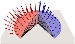
Figure 1. Sketch of a thin pinned particle-laden sessile evaporating droplet on a planar substrate. The droplet has constant contact radius  $\hat {R}_0$, contact angle $\hat {\theta }(\hat {t})$, free surface $\hat {z}=\hat {h}(\hat {r},\hat {t})$ and concentration of particles within the droplet $\hat {\phi }(\hat {r},\hat {z},\hat {t})$. The arrows indicate the local evaporative mass flux $\hat {J}(\hat {r})$.
The velocity and pressure within the droplet, denoted by  $\hat {\boldsymbol {u}}=(\hat {u}(\hat {r},\hat {z},\hat {t}),0,\hat {w}(\hat {r},\hat {z},\hat {t}))$ and $\hat {p}=\hat {p}(\hat {r},\hat {z},\hat {t})$, satisfy the usual mass-conservation and Stokes equations subject to no-slip and no-penetration conditions on the substrate and stress and kinematic conditions on the free surface of the droplet. The concentration of particles within the droplet, denoted by $\hat {\phi }=\hat {\phi }(\hat {r},\hat {z},\hat {t})$, satisfies an advection–diffusion equation subject to no-flux conditions on both the substrate and the free surface of the droplet.
The form of the local evaporative mass flux from the free surface of the droplet, denoted by  $\hat {J}=\hat {J}(\hat {r},\hat {t}) \, ({\geqslant }0)$, depends on the physical mechanism(s) controlling the evaporation (see for example Wilson & D'Ambrosio Reference Wilson and D'Ambrosio2023). In §§ 3–6 we assume that the local evaporative flux is steady and takes the general form $\hat {J}=\hat {J}(\hat {r})$, where $\hat {J}$ is a prescribed function of $\hat {r}$. Then in §§ 7 and 8 we consider a particular one-parameter family of local evaporative fluxes. In Appendix A we show how the analysis in §§ 3–6 can be generalised to the situation in which the local evaporative flux is unsteady and takes the general separable form $\hat {J}=\hat {J}(\hat {r},\hat {t})=\hat {f}(\hat {r})\hat {g}(\hat {t})$, where $\hat {f}$ and $\hat {g}$ are prescribed functions of $\hat {r}$ and $\hat {t}$, respectively, as investigated numerically by Fischer (Reference Fischer2002).
Before proceeding further, we non-dimensionalise and scale the variables appropriately for a thin droplet (i.e. in the limit of small contact angle) according to
 \begin{equation} \left.\begin{gathered}
\hat{r}=\hat{R}_0 r, \quad \hat{z}=\hat{\theta}_0\hat{R}_0
z, \quad \hat{\theta}=\hat{\theta}_0 \theta, \quad
\hat{h}=\hat{\theta}_0\hat{R}_0 h, \quad
\hat{V}=\hat{\theta}_0\hat{R}_0^3 V, \quad
\hat{t}=\frac{\hat{R}_0}{\hat{U}_{ref}} t, \\
\hat{u}=\hat{U}_{ref} u, \quad
\hat{w}=\hat{\theta}_0\hat{U}_{ref} w, \quad
\hat{p}-\hat{p}_{a}=\frac{\hat{\gamma}\hat{\theta}_0}{\hat{R}_0}
p,\quad \hat{\phi}=\hat{\phi}_{ref} \phi, \quad
\hat{J}=\hat{J}_{ref} J, \end{gathered}\right\}
\end{equation}
\begin{equation} \left.\begin{gathered}
\hat{r}=\hat{R}_0 r, \quad \hat{z}=\hat{\theta}_0\hat{R}_0
z, \quad \hat{\theta}=\hat{\theta}_0 \theta, \quad
\hat{h}=\hat{\theta}_0\hat{R}_0 h, \quad
\hat{V}=\hat{\theta}_0\hat{R}_0^3 V, \quad
\hat{t}=\frac{\hat{R}_0}{\hat{U}_{ref}} t, \\
\hat{u}=\hat{U}_{ref} u, \quad
\hat{w}=\hat{\theta}_0\hat{U}_{ref} w, \quad
\hat{p}-\hat{p}_{a}=\frac{\hat{\gamma}\hat{\theta}_0}{\hat{R}_0}
p,\quad \hat{\phi}=\hat{\phi}_{ref} \phi, \quad
\hat{J}=\hat{J}_{ref} J, \end{gathered}\right\}
\end{equation}
where  $\hat {\gamma }$ is the constant surface tension of the fluid, $\hat {p}_{a}$ is the constant atmospheric pressure, $\hat {U}_{ref}={\hat {J}_{ref}}/{(\hat {\rho }\hat {\theta }_0)}$ is an appropriate characteristic radial velocity scale, in which $\hat {\rho }$ is the constant density of the fluid, $\hat {J}_{ref}$ is an appropriate characteristic local evaporative flux scale which depends on the physical mechanism(s) controlling evaporation and $\hat {\phi }_{ref}$ is an appropriate characteristic particle concentration scale, chosen to be the spatial average of the initial concentration of particles.
In the present work we are primarily (but not exclusively) motivated by situations in which evaporation is described by the basic quasi-steady diffusion-limited model for the concentration of vapour in the atmosphere (see for example Picknett & Bexon Reference Picknett and Bexon1977; Popov Reference Popov2005; Barash et al. Reference Barash, Bigioni, Vinokur and Shchur2009; Wilson & Duffy Reference Wilson and Duffy2022; Wilson & D'Ambrosio Reference Wilson and D'Ambrosio2023), subject to a variety of different boundary conditions corresponding to, for example, surrounding the droplet with a bath of fluid or using a mask with one or more holes in it to achieve a desired pattern of evaporation enhancement and/or suppression. In particular, for the diffusion-limited evaporation of a thin droplet appropriate characteristic radial velocity and local evaporative flux scales are
 \begin{equation} \hat{U}_{ref}=\frac{\hat{D}(\hat{c}_{sat}-\hat{c}_{\infty})}{\hat{\rho}\hat{\theta}_0\hat{R}_0}, \quad \hat{J}_{ref}=\frac{\hat{D}(\hat{c}_{sat}-\hat{c}_{\infty})}{\hat{R}_0}, \end{equation}
where  $\hat {D}$ is the constant diffusion coefficient of vapour in the atmosphere, $\hat {c}_{sat}$ is the constant saturation concentration of vapour in the atmosphere and $\hat {c}_{\infty }$ is the constant ambient concentration of vapour in the atmosphere (see for example Wilson & Duffy Reference Wilson and Duffy2022). For the simplest and most widely studied case of a thin droplet evaporating into an unbounded atmosphere the local evaporative flux is given by the well-known expression
 \begin{equation} J = \frac{2}{\rm \pi}(1-r^2)^{{-}1/2}. \end{equation}
Note that the basic diffusion-limited model has been extended to include a variety of additional physical effects (such as, for example, the dependence of  $\hat {c}_{sat}$ on temperature and buoyancy-driven convection in the atmosphere) and/or to relax the assumption of quasi-steadiness, but in the present work we restrict our attention to the basic model. However, even for the basic diffusion-limited model, depending on the specific boundary conditions imposed, it may be either difficult or impossible to obtain a closed-form solution for the concentration of vapour in the atmosphere, and hence to determine a closed-form expression for the local evaporative flux. Thus, as previously mentioned, in the present work we follow an alternative (and more pragmatic) approach similar in spirit to that taken by Fischer (Reference Fischer2002) and analyse a one-parameter family of local evaporative fluxes which includes members with the same qualitative features as those found experimentally and/or hypothesised theoretically by previous authors. However, it should be noted that the results obtained in the present work do not rely on this specific motivation for the form of the local evaporative flux.
3. The evolution of the droplet
We consider the situation in which the droplet is sufficiently small that the effect of gravity is negligible, and the surface tension is sufficiently strong that the profile of the droplet evolves quasi-statically. More specifically, we consider the situation in which the appropriately defined Bond number  $\textit {Bo}$ and capillary number $\textit {Ca}$, namely
 \begin{equation} \textit{Bo}=\frac{\hat{\rho}\hat{g}\hat{R}_0^2}{\hat{\gamma}} \quad \text{and} \quad \textit{Ca}=\frac{\hat{\mu}\hat{U}_{ref}}{\hat{\theta}_0^3\hat{\gamma}}, \end{equation}
respectively, where  $\hat {g}$ is the magnitude of acceleration due to gravity and $\hat {\mu }$ is the constant dynamic viscosity of the fluid, are both small and satisfy $\hat {\theta }_0^2, \textit {Bo} \ll \textit {Ca} \ll 1$.
We seek an asymptotic solution for the pressure  $p$ in the form
 \begin{equation} p=p^{(0)}+\textit{Ca} \, p^{(1)}+O(\hat{\theta}_0^2,\textit{Bo},\textit{Ca}^2). \end{equation}
Note that the pressure  $p$ and concentration of particles $\phi$ are the only quantities that we require beyond leading order, and so, for clarity, we omit the ‘ $(0)$’ superscript on all other leading-order quantities.
At leading order, the Stokes equation yields  $\partial p^{(0)}/\partial r=\partial p^{(0)}/\partial z=0$, and hence the leading-order pressure is independent of $r$ and $z$, i.e. $p^{(0)}=p^{(0)}(t)$, and is given by the normal stress condition at the free surface to be
 \begin{equation} p^{(0)}={-}\frac{1}{r}\frac{\partial}{\partial r}\left(r\frac{\partial h}{\partial r}\right). \end{equation}
The free-surface profile of the droplet  $h(r,t)$ therefore satisfies
 \begin{equation} \frac{\partial}{\partial r}\left(\frac{1}{r}\frac{\partial}{\partial r}\left(r\frac{\partial h}{\partial r}\right)\right)=0, \end{equation}
subject to  $h=0$ and $\partial h/\partial r=-\theta$ at $r=1$ together with the requirement that $h(0,t)$ must be finite, and hence takes the familiar paraboloidal form
 \begin{equation} h=\frac{\theta(1-r^2)}{2}. \end{equation}
Evaluating (3.3) using (3.5) yields  $p^{(0)}=2\theta$. For the purpose of the present work, it is convenient to express $h$ as
 \begin{equation} h=\theta\eta, \quad \text{where} \ \eta(r)=\frac{1-r^2}{2}. \end{equation}
 The volume  $V=V(t)$ of the droplet is given by
 \begin{equation} V=2{\rm \pi}\int_0^1 h(r,t)r\,\text{d}r=2{\rm \pi}\theta H(1)=\frac{{\rm \pi}\theta}{4}, \end{equation}
where  $H=H(r)$, defined by
 \begin{equation} H=\int_0^r \eta(\tilde{r})\,\tilde{r}\,\text{d}\tilde{r}=\frac{1-(1-r^2)^2}{8}, \end{equation}
is the incomplete radial integral of  $\eta r$. For future reference we note that $H(1)=1/8$.
The droplet evolves according to the global mass-conservation condition
 \begin{equation} \frac{\text{d}V}{\text{d}t}={-}F, \end{equation}
where  $F$, defined by
 \begin{equation} F=2{\rm \pi}\int_0^1 J(\tilde{r})\,\tilde{r}\,\text{d}\tilde{r}=2{\rm \pi} I(1), \end{equation}
is the (constant) total evaporative mass flux from the free surface of the droplet, in which  $I=I(r)$, defined by
 \begin{equation} I=\int_0^r J(\tilde{r})\,\tilde{r}\,\text{d}\tilde{r}, \end{equation}
is the incomplete radial integral of  $J \, r$. The initial values of $\theta$ and $V$ are given by $\theta =\theta _0=1$ and $V=V_0={\rm \pi} /4$. Substituting the expression for $V$ given by (3.7) into (3.9) with (3.10) yields
 \begin{equation} \frac{\text{d}V}{\text{d}t}=2{\rm \pi}\frac{\text{d}\theta}{\text{d}t}H(1) ={-}2{\rm \pi} I(1), \end{equation}
and solving (3.12) shows that the droplet evolves according to
 \begin{equation} \theta=1-\frac{I(1)}{H(1)}t, \quad V=\frac{\rm \pi}{4}\left(1-\frac{I(1)}{H(1)}t\right). \end{equation}
Setting  $V=0$ in (3.13a,b) shows that the lifetime of the droplet is given by
 \begin{equation} t_{lifetime}=\frac{H(1)}{I(1)}. \end{equation}
Note that in the special case of diffusion-limited evaporation into an unbounded atmosphere for which  $J$ is given by (2.3), (3.11) yields $I(1)=2/{\rm \pi}$, (3.10) gives $F=2{\rm \pi} I(1)=4$ and (3.14) recovers the familiar expression for the lifetime of a thin pinned droplet, namely $t_{lifetime}={\rm \pi} /16$ (see for example Stauber et al. Reference Stauber, Wilson, Duffy and Sefiane2014; Wilson & Duffy Reference Wilson and Duffy2022).
4. The flow within the droplet
At leading order the mass-conservation equation is
 \begin{equation} \frac{1}{r}\frac{\partial (ru)}{\partial r}+\frac{\partial w}{\partial z}=0, \end{equation}
and at first order the Stokes equation reduces to
 \begin{equation} \frac{\partial^2u}{\partial z^2}=\frac{\partial p^{(1)}}{\partial r}, \quad 0=\frac{\partial p^{(1)}}{\partial z} \end{equation}
(see for example Wray et al. Reference Wray, Wray, Duffy and Wilson2021). In particular, (4.2b) shows that the first-order pressure  $p^{(1)}$ is independent of $z$, i.e. $p^{(1)}=p^{(1)}(r,t)$. Solving (4.1) and (4.2) subject to the no-slip and no-penetration conditions on the substrate, i.e. $u(r,0,t)=w(r,0,t)=0$, and the tangential stress condition on the free surface of the droplet,
 \begin{equation} \frac{\partial u}{\partial z}=0 \quad \text{on} \ z=h, \end{equation}
leads to
 \begin{equation} u=\frac{1}{2}\frac{\partial p^{(1)}}{\partial r}\left(z^2-2hz\right)\end{equation}
and
 \begin{equation} w=\frac{z^2}{6r}\left[\frac{\partial p^{(1)}}{\partial r}\left(3r\frac{\partial h}{\partial r}+3h-z\right)+\frac{\partial^2p^{(1)}}{\partial r^2}r\left(3h-z\right)\right]. \end{equation}
The kinematic condition can be expressed as
 \begin{equation} \frac{\partial h}{\partial t}+\frac{1}{r}\frac{\partial (rQ)}{\partial r}={-}J, \end{equation}
where  $Q=Q(r,t)$, defined by
 \begin{equation} Q=\int_0^h u\,\text{d}z=h\bar{u}, \end{equation}
is the local radial volume flux of fluid, and  $\bar {u}=\bar {u}(r,t)$, defined by
 \begin{equation} \bar{u}=\frac{1}{h}\int_0^h u\,\text{d}z, \end{equation}
is the depth-averaged radial velocity. Substituting the expression for  $u$ given by (4.4) into (4.7) yields
 \begin{equation} Q={-}\frac{h^3}{3}\frac{\partial p^{(1)}}{\partial r}. \end{equation}
For the purpose of the present work, it is convenient to express  $Q$ in terms of the incomplete integrals $H$ and $I$ given by (3.8) and (3.11), respectively, by integrating (4.6) with respect to $r$ and rearranging to give
 \begin{equation} Q={-}\frac{1}{r}\int_0^r \left(J+\frac{\partial h}{\partial t}\right)\tilde{r}\,\text{d}\tilde{r} ={-}\frac{1}{r}\left(\int_0^r J(\tilde{r})\,\tilde{r}\,\text{d}\tilde{r} +\frac{\text{d}\theta}{\text{d}t}\int_0^r \eta(\tilde{r})\,\tilde{r}\,\text{d}\tilde{r}\right), \end{equation}
and hence obtaining the explicit expression
 \begin{equation} Q=\frac{I(1)H(r)-H(1)I(r)}{rH(1)}. \end{equation}
In particular, (4.11) shows that  $Q$ (but not, of course, $\bar {u}$) is independent of time $t$. Eliminating $Q$ between (4.9) and (4.11) and recalling that $h$ is given by (3.5) gives
 \begin{equation} \frac{\partial p^{(1)}}{\partial r}={-}\frac{24\left[I(1)H(r)-H(1)I(r)\right]}{\theta^3r(1-r^2)^3H(1)}, \end{equation}
and explicit expressions for the velocities  $u$ and $w$ are given by substituting (4.12) into (4.4) and (4.5).
5. The concentration of particles within the droplet
The concentration of particles within the droplet  $\phi$ satisfies the advection–diffusion equation
 \begin{equation} \textit{Pe}^*\left(\frac{\partial \phi}{\partial t}+u\frac{\partial \phi}{\partial r}+w\frac{\partial\phi}{\partial z}\right) =\hat{\theta}_0^2\frac{1}{r}\frac{\partial}{\partial r}\left(r\frac{\partial\phi}{\partial r}\right)+\frac{\partial^2 \phi}{\partial z^2}, \end{equation}
in which  $\textit {Pe}^*$ is the appropriately defined reduced Péclet number which characterises the ratio of advective and diffusive particle transport timescales, namely
 \begin{equation} \textit{Pe}^*=\frac{\hat{\theta}_0^2\hat{R}_0\hat{U}_{ref}}{\hat{D}_{p}}, \end{equation}
where  $\hat {D}_{p}$ is the constant diffusivity of the particles in the fluid. Equation (5.1) is subject to the no-flux conditions
 \begin{equation} \frac{\partial\phi}{\partial z}=0 \quad \text{on} \ z=0\end{equation}
and
 \begin{equation} \frac{1}{\sqrt{1+\hat{\theta}_0^2\left({\partial h}/{\partial r}\right)^2}} \left(\frac{\partial\phi}{\partial z}-\hat{\theta}_0^2\frac{\partial h}{\partial r}\frac{\partial\phi}{\partial r}\right) =\textit{Pe}^* J \phi \quad \text{on} \ z=h. \end{equation}
 In most of the remainder of the present work we consider the regime in which diffusion is faster than axial advection but slower than radial advection, i.e. we consider the regime in which the reduced Péclet number satisfies  $\hat {\theta }_0^2\ll \textit {Pe}^*\ll 1$, and seek an asymptotic solution for $\phi$ in the form
 \begin{equation} \phi=\phi^{(0)}+\textit{Pe}^*\phi^{(1)}+O\left(\hat{\theta}_0^2,{\textit{Pe}^*}^2\right). \end{equation}
However, note that in § 8 we calculate the paths of the particles in the alternative regime in which diffusion is slower than both axial and radial advection, i.e. when the reduced Péclet number satisfies  $\textit {Pe}^*\gg 1$.
At leading order, (5.1), (5.3) and (5.4) reduce to
 \begin{equation} \frac{\partial^2\phi^{(0)}}{\partial z^2}=0, \end{equation}
subject to
 \begin{equation} \frac{\partial\phi^{(0)}}{\partial z}=0\quad \text{on} \ z=0 \ \text{and}\ z=h, \end{equation}
which shows that  $\phi ^{(0)}$ is independent of $z$, i.e. $\phi ^{(0)}=\phi ^{(0)}(r,t)$.
At first order, (5.1), (5.3) and (5.4) reduce to
 \begin{equation} \frac{\partial^2\phi^{(1)}}{\partial z^2}=\frac{\partial\phi^{(0)}}{\partial t}+u\frac{\partial\phi^{(0)}}{\partial r}, \end{equation}
subject to
 \begin{equation} \frac{\partial\phi^{(1)}}{\partial z}=0 \quad \text{on} \ z=0 \end{equation}
and
 \begin{equation}\frac{\partial\phi^{(1)}}{\partial z}=J \phi^{(0)} \quad \text{on} \ z=h. \end{equation}
Integrating (5.8) with respect to  $z$ subject to (5.9) and (5.10), and henceforth dropping the superscript ‘ $(0)$’ on $\phi$ for clarity, yields the equation for the leading-order concentration of particles, namely
 \begin{equation} \frac{\partial\phi}{\partial t} +\bar{u}\frac{\partial\phi}{\partial r}=\frac{J \phi}{h}, \end{equation}
where the depth-averaged radial velocity  $\bar {u}$ is given by (4.8) (see for example Deegan et al. Reference Deegan, Bakajin, Dupont, Huber, Nagel and Witten2000; Wray et al. Reference Wray, Papageorgiou, Craster, Sefiane and Matar2014, Reference Wray, Wray, Duffy and Wilson2021).
Equation (5.11) may be put into characteristic form, i.e.
 \begin{equation} \frac{\text{d}\phi}{\text{d}t}=\frac{J \phi}{h} \quad \text{on the characteristics determined by} \quad \frac{\text{d}r}{\text{d}t}=\bar{u}, \end{equation}
subject to a prescribed initial concentration of particles in the bulk of the droplet,  $\phi (r,0)=\phi _0(r)$, and solved using the method of characteristics. Using the expressions for $h$ and $\textrm {d}\theta /\textrm {d}t$ given by (3.6) and (3.12), the characteristic equations (5.12) can be used to write
 \begin{equation} \frac{\text{d}r}{\text{d}\theta} =\frac{\text{d}r/\text{d}t}{\text{d}\theta/\text{d}t} ={-}\frac{H(1)Q(r)}{\theta I(1)\eta(r) }, \quad \frac{\text{d}\phi}{\text{d}r} =\frac{\text{d}\phi/\text{d}t}{\text{d}r/\text{d}t} =\frac{J(r)\phi}{Q(r)}. \end{equation}
Integration of (5.13a,b) yields the implicit solution
 \begin{equation} \log{\theta}={-}\int_{r_0}^r \frac{I(1)\eta(\tilde{r})}{H(1)Q(\tilde{r})}\,\text{d}\tilde{r}, \quad \log{\frac{\phi}{\phi_0}}=\int_{r_0}^r \frac{J(\tilde{r})}{Q(\tilde{r})}\,\text{d}\tilde{r}, \end{equation}
where  $r_0=r_0(r,t)$ $(0 \leqslant r_0 \leqslant 1)$ denotes the initial radial position (i.e. the radial position at time $t=0$) of the particles that are at radial position $r$ at time $t$ (see for example Boulogne et al. Reference Boulogne, Ingremeau and Stone2017), and is determined by solving (5.14a). Note that, by definition, $r_0(r,0)=r$. The solution (5.14) can be simplified by adding (5.14a) and (5.14b) to yield
 \begin{equation} \log{\theta}+\log{\frac{\phi}{\phi_0}} ={-}\int_{r_0}^r \frac{I(1)\eta(\tilde{r})-H(1)J(\tilde{r})}{H(1)Q(\tilde{r})}\,\text{d}\tilde{r}, \end{equation}
and then recalling that  $Q$ may be expressed in the form (4.11) to give
 \begin{equation} \log{\theta}+\log{\frac{\phi}{\phi_0}} ={-}\int_{r_0}^r \frac{1}{\tilde{r}Q(\tilde{r})}\frac{\text{d}\left(\tilde{r}Q(\tilde{r})\right)}{\text{d}\tilde{r}}\,\text{d}\tilde{r} =\log{\frac{r_0Q(r_0)}{rQ(r)}}. \end{equation}
Hence the implicit solution (5.14) of the characteristic equations (5.12) may be written in the simplified form
 \begin{equation} \log{\theta}={-}\int_{r_0}^r \frac{I(1)\eta(\tilde{r})}{H(1)Q(\tilde{r})}\,\text{d}\tilde{r}, \quad\frac{\phi}{\phi_0}=\frac{r_0Q(r_0)}{\theta rQ(r)}. \end{equation}
As mentioned in § 2, the corresponding analysis for the situation in which the local evaporative flux is unsteady and takes a general separable form is described in Appendix A.
6. The mass of particles
The mass of particles per unit area within the footprint of the droplet is  $\phi h$, and so the mass of particles in the bulk of the droplet as it evaporates, denoted by $M_{drop}=M_{drop}(t)$ (non-dimensionalised by $\hat {\theta }_0\hat {R}_0^3\hat {\phi }_{ref}$), is given by
 \begin{equation} M_{drop}=2{\rm \pi}\int_0^1 \phi(r,t)\,h(r,t)\,r\,\text{d}r, \end{equation}
which can be rewritten as
 \begin{equation} M_{drop}=2{\rm \pi}\int_0^{r_0(1,t)} \phi_0(r)\,h(r,0)\,r\,\text{d}r, \end{equation}
where  $r_0(1,t)$ denotes the initial radial position of the particles that are at radial position $r=1$ (i.e. at the contact line) at time $t$, which is determined by solving (5.17a) with $r=1$. The initial mass of particles in the droplet is $M_{drop}(0)=M_0$, where
 \begin{equation} M_0=2{\rm \pi}\int_0^1 \phi_0(r)\,h(r,0)\,r\,\text{d}r. \end{equation}
 The mass flux of particles from the bulk of the droplet into the contact line is  $\lim _{r \to 1^-} 2 {\rm \pi}r \phi Q$, and so the mass of particles in the ring deposit that can form at the contact line, denoted by $M_{ring}=M_{ring}(t)$ (also non-dimensionalised by $\hat {\theta }_0\hat {R}_0^3\hat {\phi }_{ref}$), is given by
 \begin{equation} M_{ring}=2{\rm \pi}\int_0^t \lim_{r \to 1^-} r\,\phi(r,\tilde{t})\,Q(r,\tilde{t})\,\text{d}\tilde{t}, \end{equation}
which can be rewritten as
 \begin{equation} M_{ring}=2{\rm \pi}\int_{r_0(1,t)}^1 \phi_0(r)\,h(r,0)\,r\,\text{d}r \end{equation}
(see Deegan et al. Reference Deegan, Bakajin, Dupont, Huber, Nagel and Witten2000; Boulogne et al. Reference Boulogne, Ingremeau and Stone2017). The initial mass of particles in the ring is, by definition, zero, i.e.  $M_{ring}(0)=0$.
Adding the expressions for  $M_{drop}$ and $M_{ring}$, given by (6.2) and (6.5), respectively, confirms that the total mass of particles is conserved as the droplet evaporates, i.e. that $M_{drop}+M_{ring} \equiv M_0$.
For simplicity, in the remainder of the present work we take the initial concentration of particles in the bulk of the droplet to be spatially uniform, and so, as consequence of our choice of  $\hat {\phi }_{ref}$, $\phi _0(r) \equiv 1$. In this case, from (6.3), the initial mass of particles in the droplet is
 \begin{equation} M_0=2{\rm \pi}\int_0^1 h(r,0)\,r\,\text{d}r=\frac{\rm \pi}{4}. \end{equation}
7. A one-parameter family of local evaporative fluxes
7.1. The local evaporative flux
In the remainder of the present work we analyse the behaviour of the general solutions obtained in §§ 3–6 for a one-parameter family of local evaporative fluxes of the form  $J(r)=J_0(1-r^2)^n$, where, in order to ensure that the total evaporative flux given by (3.10) is finite, the exponent $n$ must satisfy $n>-1$, but is otherwise a free parameter. As mentioned in § 2, this specific form of $J$ was chosen because as $n$ is varied it exhibits qualitatively different behaviours mimicking those that can be obtained by, for example, surrounding the droplet with a bath of fluid or using a mask with one or more holes in it to achieve a desired pattern of evaporation enhancement and/or suppression, as described in § 1. (Note that a similar, but different, variation in the form of $J$ occurs as the contact angle varies over the range $0 < \theta \leqslant {\rm \pi}$.) In particular, the values $n=-1/2$, $n=0$ and $n=1$ correspond to diffusion-limited evaporation into an unbounded atmosphere given by (2.3), spatially uniform evaporation and evaporation that is proportional to $-\partial h/\partial t$, respectively. However, as also mentioned in § 2, the rather general results obtained in the present work do not rely exclusively on this specific motivation for the form of the local evaporative flux.
To facilitate comparison between the results for different values of  $n$, the pre-factor in $J$ was chosen to be $J_0=J_0(n)=4(n+1)/{\rm \pi}$ so that the total evaporative flux given by (3.10) is equal to its value for diffusion-limited evaporation into an unbounded atmosphere, namely $F=4$, for all values of $n$. In particular, this means that the evolution of the droplet given by (3.13), namely
 \begin{equation} \theta=1-\frac{16}{\rm \pi}t, \quad V=\frac{\rm \pi}{4}-4t, \end{equation}
and hence the lifetime of the droplet given by (3.14), namely  $t_{lifetime}={\rm \pi} /16$, are the same for all values of $n$. Thus in the remainder of the present work we take
 \begin{equation} J(r)=\frac{4(n+1)}{\rm \pi}(1-r^2)^n \quad \mbox{for} \ n>{-}1, \end{equation}
and, in particular, we will describe the qualitatively different behaviours of the flow within the droplet in § 7.2, the concentration of particles within the droplet in § 7.3 and the masses of the particles in the bulk of the droplet and in the ring deposit in § 7.4 for different values of  $n$.
$n$.
Figure 2 shows  $J$ given by (7.2) plotted as a function of $r$ for a range of values of $n$. As figure 2 shows, the behaviour of $J$ is qualitatively different for $-1< n<0$, $n=0$, and $n>0$. For $-1< n<0$ (including the special case $n=-1/2$ of diffusion-limited evaporation into an unbounded atmosphere), $J$ is a monotonically increasing function of $r$ which takes its minimum value at the centre of the droplet (i.e. at $r=0$) and is (integrably) singular at the contact line (i.e. at $r=1$) according to
 \begin{equation} J \sim \frac{2^{2+n}(n+1)}{\rm \pi}(1-r)^n \quad \hbox{as} \ r \to 1^-. \end{equation}
For  $n=0$ (i.e. spatially uniform evaporation), $J \equiv 4/{\rm \pi}$, while for $n>0$ (including the special case $n=1$ in which $J$ is proportional to $-\partial h/\partial t$), $J$ is a monotonically decreasing function of $r$ which takes its maximum value at the centre of the droplet and approaches zero at the contact line according to (7.3).

Figure 2. The prescribed local evaporative flux  $J$ given by (7.2) plotted as a function of $r$ for (a) $n=-3/4, -1/2, \ldots, 3$ and (b) $n=4, 8, \ldots, 40$. In (a) the dashed line denotes the curve for $n=1$. The arrows indicate the direction of increasing $n$.
$n$.
7.2. The flow within the droplet
Substituting the expression for  $J$ given by (7.2) into (3.11) and evaluating the integral gives
 \begin{equation} I=\frac{4(n+1)}{\rm \pi}\int_0^r (1-\tilde{r}^2)^n\,\tilde{r}\,\text{d}\tilde{r} =\frac{2}{\rm \pi}\left[1-(1-r^2)^{n+1}\right], \end{equation}
and so from (4.11) with (3.8) and (7.4) the radial volume flux  $Q$ is given by
 \begin{equation} Q=\frac{2(1-r^2)}{{\rm \pi} r}\left[(1-r^2)^n-(1-r^2)\right], \end{equation}
and hence the depth-averaged radial velocity  $\bar {u}$ is given by
 \begin{equation} \bar{u}=\frac{Q}{h}=\frac{4}{{\rm \pi}\theta r}\left[(1-r^2)^n-(1-r^2)\right]. \end{equation}
 In the special case  $n=1$ (7.5) and (7.6) give $Q \equiv 0$ and $\bar {u} \equiv 0$, and, as we shall show subsequently, there is no flow within the droplet in this case.
Figures 3 and 4 show  $Q$ given by (7.5) and $\bar {u}\theta$ given by (7.6), respectively, for a range of values of $n$. In particular, figures 3 and 4 show that both $Q$ and $\bar {u}$ are qualitatively different for $-1< n<1$ and $n>1$. Specifically, for $-1< n<1$ the average radial velocity is always outwards (i.e. $Q \geqslant 0$ and $\bar {u} \geqslant 0$), whereas for $n>1$ the average radial velocity is always inwards (i.e. $Q \leqslant 0$ and $\bar {u} \leqslant 0$). However, figures 3 and 4 also show that while $Q$ always approaches zero at $r=0$ and $r=1$ and $\bar {u}$ always approaches zero at $r=0$ according to $\bar {u} \sim 4(1-n)r/({\rm \pi} \theta ) \to 0$ as $r \to 0^+$, the behaviour of $\bar {u}$ at $r=1$ is more complicated. Specifically, for $-1< n<0$, $\bar {u}$ is singular according to
 \begin{equation} \bar{u} \sim \frac{2^{2+n}}{{\rm \pi}\theta}(1-r)^n \quad \hbox{as} \ r \to 1^-, \end{equation}
for  $n=0$, $\bar {u}=4/({\rm \pi} \theta )$ at $r=1$, for $0< n<1$, $\bar {u}$ approaches zero from above according to (7.7), while for $n \geqslant 1$, $\bar {u}$ approaches zero from below according to
 \begin{equation} \bar{u} \sim{-}\frac{8}{{\rm \pi}\theta}(1-r) \to 0^- \quad \hbox{as} \ r \to 1^-. \end{equation}
Figure 3. The radial volume flux  $Q$ given by (7.5) plotted as a function of $r$ for (a) $n=-3/4, -1/2, \ldots, 1$ and (b) $n=2, 4, \ldots, 20$. In (a) the dashed line denotes the limiting value of $Q$ as $n \to -1^+$, namely $2r(2-r^2)/{\rm \pi}$. The arrows indicate the direction of increasing $n$.
$n$.

Figure 4. The quantity  $\bar {u}\theta$ given by (7.6) plotted as a function of $r$ for (a) $n=-3/4, -1/2, \ldots, 1$ and (b) $n=2, 4, \ldots, 20$. In (a) the dashed line denotes the limiting value of $\bar {u}\theta$ as $n \to -1^+$, namely $4r(2-r^2)/ ({\rm \pi} (1-r^2))$. The arrows indicate the direction of increasing $n$.
$n$.
Substituting the expression for  $\partial p^{(1)}/\partial r$ given by (4.12) into (4.4) and (4.5) yields the solutions for the velocities $u$ and $w$, namely
 \begin{equation} u=\frac{24z}{{\rm \pi}\theta^3 r (1-r^2)^2} \left[(1-r^2)^n-(1-r^2)\right]\left[\theta(1-r^2)-z\right]\end{equation}
and
 \begin{align} w={-}\frac{8z^2}{{\rm \pi}\theta^3(1-r^2)^3} \left[3\theta(1-n)(1-r^2)^{n+1}-2(2-n)(1-r^2)^nz+2(1-r^2)z\right], \end{align}
with (Stokes) streamfunction  $\psi =\psi (r,z,t)$ (non-dimensionalised by $\hat {R}_0\hat {U}_{ref}$)
 \begin{equation} \psi={-}\frac{4z^2}{{\rm \pi}\theta^3 (1-r^2)^2} \left[(1-r^2)^n-(1-r^2)\right]\left[3\theta(1-r^2)-2z\right]. \end{equation}
In particular, (7.9) shows that the radial velocity  $u$ satisfies $u>0$, $u \equiv 0$ and $u<0$ everywhere within the droplet when $-1< n<1$, $n=1$ and $n>1$, respectively, i.e. the radial velocity is always in the same direction as the average radial velocity. However, as (7.10) shows, the behaviour of the vertical velocity $w$ is qualitatively different for $-1 < n \leqslant 1/2$, $1/2 < n < 1$, $n=1$ and $n > 1$. Specifically, whereas $w<0$ and $w \equiv 0$ everywhere within the droplet when $-1 < n \leqslant 1/2$ and $n=1$, respectively, the sign of $w$ is not the same everywhere within the droplet when $1/2 < n < 1$ and when $n>1$, i.e. there is always both upwards and downwards flow in these cases. Using (7.10) shows that in these cases there is a curve within the droplet on which $w=0$, denoted by $z=z_{crit}(r,t)$, given by
 \begin{equation} \frac{z_{crit}}{h}=\frac{3(1-n)}{2-n-(1-r^2)^{1-n}} \quad \hbox{for} \ r_{crit} \leqslant r \leqslant 1, \end{equation}
where  $r=r_{crit}$ is the solution of $z_{crit}/h=1$. Specifically, when $1/2 < n < 1$ then $w<0$ everywhere within the droplet except for $w=0$ on $z = z_{crit}$ and $w>0$ for $z_{crit} < z \leqslant h$ and, conversely, when $n > 1$ then $w>0$ everywhere within the droplet except for $w=0$ on $z = z_{crit}$ and $w<0$ for $z_{crit} < z \leqslant h$.
In the special cases  $n=-1/2$ and $n=0$ (7.9) and (7.10) are equivalent to the corresponding expressions given by Boulogne et al. (Reference Boulogne, Ingremeau and Stone2017). In the special case $n=1$ (7.9) and (7.10) give $u \equiv 0$ and $w \equiv 0$, i.e. the local mass loss due to evaporation is exactly balanced by the local decrease of the free-surface profile everywhere, and so there is no flow within the droplet.
Note that while  $J$ and $Q$ are independent of time $t$, the quantities $\bar {u}$, $u$ and $w$ all depend on $t$ via their dependence on $\theta$ given by (7.1a). In particular, $\bar {u}$ is singular in the limit $t \to t_{lifetime}^-$ with $\bar {u} \to +\infty$ for $-1< n<1$ and $\bar {u} \to -\infty$ for $n>1$, where the former behaviour is a generalisation of the rush-hour effect that occurs during the final stages of diffusion-limited evaporation into an effectively unbounded atmosphere mentioned in § 1.
The solution for the first-order pressure  $p^{(1)}$ can be obtained by eliminating $Q$ between (4.9) and (7.5) and integrating with respect to $r$. The resulting expression for $p^{(1)}$ is given by D'Ambrosio (Reference D'Ambrosio2022), but is rather cumbersome and so is omitted here for brevity.
Figure 5 shows the instantaneous streamlines of the flow within the droplet calculated from (7.9) and (7.10) for (a)  $n=-1/2$ (typical of $-1 < n \leqslant 1/2$) and (b) $n=4$ (typical of $n > 1$) at $t=t_{lifetime}/2={\rm \pi} /32$. (Note that, for brevity, figure 5 does not include a corresponding plot for a value of $n$ in the range $1/2< n<1$.) In particular, figure 5(a) illustrates that when $n=-1/2$ the flow is outwards and downwards everywhere, while figure 5(b) illustrates that when $n=4$ the flow is inwards and upwards everywhere except for a region of downwards flow for $z_{crit} < z \leqslant h$ when $r_{crit} \simeq 0.6908 < r < 1$, where the curve $z=z_{crit}$ on which $w=0$ is given by (7.12).


7.3. The concentration of particles within the droplet
Substituting the expression for  $Q$ given by (7.5) into (5.17a) and evaluating the integral gives
 \begin{equation} \theta^{(1-n)/2}=\frac{1-(1-r_0^2)^{1-n}}{1-(1-r^2)^{1-n}}, \end{equation}
and so, using (7.1a), the time for the particles that are at initial radial position  $r_0$ to reach radial position $r$ is given by
 \begin{equation} \frac{t}{t_{lifetime}}=1-\left[\frac{1-(1-r_0^2)^{1-n}}{1-(1-r^2)^{1-n}}\right]^{2/(1-n)}. \end{equation}
In particular, setting  $r=1$ in (7.14), the time for the particles that are at initial radial position $r_0$ to reach the ring deposit at the contact line, denoted by $t=t_{ring}$, is given by
 \begin{equation} \frac{t_{ring}}{t_{lifetime}}=1-\left[1-(1-r_0^2)^{1-n}\right]^{2/(1-n)} \quad \hbox{for} \ -1< n<1. \end{equation}
 Figure 6 shows  $t_{ring}/t_{lifetime}$ given by (7.15) plotted as a function of $r_0$ for various values of $n$ in the range $-1< n<1$. In particular, figure 6 shows that, as expected, $t_{ring}/t_{lifetime}$ decreases monotonically from $t_{ring}/t_{lifetime}=1$ at $r_0=0$ to $t_{ring}/t_{lifetime}=0$ at $r_0=1$, i.e. particles initially close to the contact line are deposited at the contact line before those that are initially further away from it, and all of the particles are eventually transferred from the bulk of the droplet to the ring deposit at the contact line.

Figure 6. The quantity  $t_{ring}/t_{lifetime}$ given by (7.15) as a function of $r_0$ for $n=-3/4, -1/2, \ldots, 3/4$. The dashed line denotes the limiting value of $t_{ring}/t_{lifetime}$ as $n \to -1^+$, namely $(1-r_0^2)^2$. The arrow indicates the direction of increasing $n$.
$n$.
Substituting the expression for  $Q$ given by (7.5) into (5.17b) and using (7.13) gives
 \begin{equation} \phi=\theta^{-(1+n)/2}\left(\frac{1-r_0^2}{1-r^2}\right)^{n+1}, \end{equation}
and eliminating  $r_0$ between (7.13) and (7.16) yields an explicit expression for the concentration of particles within the droplet, namely
 \begin{equation} \phi=\left[\frac{\theta^{(n-1)/2}-1+(1-r^2)^{1-n}}{(1-r^2)^{1-n}}\right]^{(n+1)/(1-n)}. \end{equation}
In the special cases  $n=-1/2$ and $n=0$ (7.17) is equivalent to the corresponding expressions given by Zheng (Reference Zheng2009).
Figure 7 shows  $\phi$ given by (7.17) plotted as a function of $r$ for a range of values of $n$ at $t=t_{lifetime}/2={\rm \pi} /32$. In particular, figure 7 illustrates that the behaviour of $\phi$ is qualitatively different for $-1< n<1$, $n=1$ and $n>1$. Specifically, for $-1< n<1$, $\phi$ is a monotonically increasing function of $r$ which takes its minimum value at $r=0$ and is singular at the contact line according to $\phi = O((1-r)^{-(n+1)})$, for $n=1$, $\phi$ remains spatially uniform and is given by $\phi =1/\theta$, while for $n>1$, $\phi$ is a monotonically decreasing function of $r$ which takes its maximum value at $r=0$ and approaches unity from above at the contact line according to $\phi =1+O((1-r)^{n-1})$.

Figure 7. The concentration of particles within the droplet  $\phi$ given by (7.17) plotted as a function of $r$ for (a) $n=-3/4, -1/2, \ldots, 1$ and (b) $n=3/2, 2, \ldots, 6$ at $t=t_{lifetime}/2={\rm \pi} /32$. The dashed lines denote the initial concentration of particles, namely $\phi \equiv 1$, which is also the limiting value of $\phi$ as $n \to -1^+$. The arrows indicate the direction of increasing $n$.
$n$.
7.4. The mass of particles
From (3.5) and (7.17) the mass of particles per unit area is given by
 \begin{equation} \phi h=\frac{\theta(1-r^2)}{2}\left[\frac{\theta^{(n-1)/2}-1+(1-r^2)^{1-n}}{(1-r^2)^{1-n}}\right]^{(n+1)/(1-n)}. \end{equation}
 Figure 8 shows  $\phi h$ given by (7.18) plotted as a function of $r$ at various times for (a) $n=-1/2$ (typical of $-1< n<0$), (b) $n=0$, (c) $n=1/2$ (typical of $0< n<1$) and (d) $n=2$ (typical of $n>1$). Note that, because it is independent of time $t$, the plot of $\phi h$ in the special case $n=1$ in which it remains identically equal to its initial value of $(1-r^2)/2$ is omitted from figure 8. In particular, figure 8 illustrates that, in addition to the special case $n=1$, the behaviour of $\phi h$ is qualitatively different for $-1< n<0$, $n=0$, $0< n<1$ and $n>1$. Specifically, figures 8(a)–8(c) illustrate that for $-1< n<1$ (i.e. when the radial flow is outwards) $\phi h$ decreases (relative to its initial value) near the centre of the droplet but increases (again relative to its initial value) near the contact line as the droplet evaporates. However, its behaviour near the contact line depends on the value of $n$, namely $\phi h = O((1-r)^{-n}) \to 0^+$ in the limit $r \to 1^-$ when $-1< n<0$, $\phi h = \theta ^{1/2}(1-\theta ^{1/2})/2 = O(1)$ at $r=1$ when $n=0$ and $\phi h = O((1-r)^{-n}) \to +\infty$ in the limit $r \to 1^-$ when $0< n<1$. Since particles are advected towards the contact line by the outwards radial flow, at first sight, the behaviour of $\phi h$ near the contact line when $-1< n<1$ might appear to be surprising. However, this behaviour is explained by the fact that when $-1< n<0$ the advection of particles towards the contact line is balanced by the flux into the ring deposit, and hence $\phi h=0$ at $r=1$, whereas when $0 \leqslant n < 1$ the advection of particles towards the contact line exceeds the flux into the ring deposit, and hence $\phi h=O(1)$ at $r=1$ when $n=0$ and $\phi h$ is unbounded in the limit $r \to 1^-$ when $0< n<1$. On the other hand, figure 8(d) illustrates that for $n>1$ (i.e. when the radial flow is inwards) $\phi h$ increases (relative to its initial value) near the centre of the droplet but decreases (again relative to its initial value) near the contact line as the droplet evaporates, and satisfies $\phi h=O(1-r) \to 0^+$ in the limit $r \to 1^-$.

Figure 8. The mass of particles per unit area  $\phi h$ given by (7.18) at times $t=(0,1/10,\ldots,9/10)\times t _{lifetime}$ for (a) $n=-1/2$, (b) $n=0$, (c) $n=1/2$ and (d) $n=2$. The dashed lines denote the initial mass of particles given by $h(r,0)=(1-r^2)/2$, and the arrows indicate the direction of increasing $t$.
$t$.
For  $n \geqslant 1$ the radial flow is always inwards (or, in the special case $n=1$, zero) and so all of the particles remain within the bulk of the droplet as it evaporates. Hence
 \begin{equation} M_{drop} \equiv M_0, \quad M_{ring} \equiv 0 \quad \hbox{for} \ n \geqslant 1, \end{equation}
and no ring deposit forms at the contact line. For  $n>1$ all of the particles are eventually advected to the centre of the droplet, and so the final deposit on the substrate predicted by the model is a deposit of mass $M_0$ at $r=0$. Of course, in practice, diffusion in the radial direction, or other weak physical effects not accounted for in the present leading-order model, will smooth this out to create a deposit of non-zero radius near $r=0$.
In the special case  $n=1$ there is no flow, and so all of the particles are simply deposited onto the substrate at their initial radial position. As a consequence of the paraboloidal shape of the initial free-surface profile of the droplet, and hence of the initial distribution of mass, the distribution of mass in the final deposit on the substrate predicted by the model is also paraboloidal, specifically $(1-r^2)/2$. This behaviour is consistent with the corresponding experimental results of Deegan et al. (Reference Deegan, Bakajin, Dupont, Huber, Nagel and Witten2000) for a local evaporative flux that is approximately proportional to the rate of decrease of the height of the droplet discussed in § 1.
For  $-1< n<1$ the radial flow is always outwards and all of the particles are eventually advected to the contact line. Evaluating $M_{drop}$ and $M_{ring}$ using (6.2) and (6.5), respectively, requires the value of $r_0(1,t)$, i.e. the initial radial position of the particles that are at radial position $r=1$ at time $t$, and this is readily obtained from (7.13) to be
 \begin{equation} r_0(1,t)=\left[1-\left(1-\theta^{(1-n)/2}\right)^{1/(1-n)}\right]^{1/2} \quad \hbox{for} \ -1< n<1. \end{equation}
Substituting the expression for  $\phi h$ given by (7.18) into (6.2) and (6.5), and evaluating the integrals using (7.20), yields explicit expressions for the masses of the particles in the bulk of the droplet and in the ring deposit at time $t$, namely
 \begin{equation} M_{drop}=M_0\left[1-\left(1-\theta^{(1-n)/2}\right)^{2/(1-n)}\right] \quad \hbox{for} \ 1< n<1\end{equation}
and
 \begin{equation} M_{ring}=M_0\left(1-\theta^{(1-n)/2}\right)^{2/(1-n)} \quad \hbox{for} \ -1< n<1, \end{equation}
respectively, where the initial mass of particles in the bulk of the droplet is given by (6.6) to be  $M_0={\rm \pi} /4$. In the special case $n=-1/2$ (7.22) is equivalent to the corresponding expression first given by Deegan et al. (Reference Deegan, Bakajin, Dupont, Huber, Nagel and Witten2000), and in the special cases $n=-1/2$ and $n=0$ it is equivalent to the corresponding expressions given by Boulogne et al. (Reference Boulogne, Ingremeau and Stone2017). For $-1< n<1$ all of the particles are eventually transferred from the bulk of the droplet to the ring deposit at the contact line, and so the final deposit on the substrate predicted by the model is a ring deposit with mass $M_0$ at $r=1$. This behaviour is consistent with the corresponding experimental results of Deegan et al. (Reference Deegan, Bakajin, Dupont, Huber, Nagel and Witten2000) and Boulogne et al. (Reference Boulogne, Ingremeau and Stone2017) for both diffusion-limited evaporation into an effectively unbounded atmosphere and approximately spatially uniform evaporation discussed in § 1. Of course, in practice, weak physical effects not accounted for in the present leading-order model will again smooth this out to create a ring deposit of non-zero width near $r=1$.
Figure 9 shows the evolutions of  $M_{drop}/M_0$ and $M_{ring}/M_0$ plotted as functions of $t/t_{lifetime}$ for various values of $n$ in the range $-1< n\leqslant 1$. In particular, figure 9(a) shows that, as expected, for $-1< n<1$, $M_{drop}/M_0$ decreases monotonically from $M_{drop}/M_0=1$ at $t/t_{lifetime}=0$ to $M_{drop}/M_0=0$ at $t/t_{lifetime}=1$, and figure 9(b) shows the corresponding behaviour of $M_{ring}/M_0$, confirming that for $-1< n<1$, all of the particles are eventually transferred from the bulk of the droplet to the ring deposit at the contact line. Figure 9 also shows that as $n$ increases from $n=-1$ towards $n=1$ the flux of particles into the ring deposit becomes increasingly concentrated towards the end of the lifetime of the droplet, i.e. the rush-hour effect becomes more and more dramatic.

Figure 9. The evolutions of (a)  $M_{drop}/M_0$ given by (7.21) and (b) $M_{ring}/M_0$ given by (7.22) as functions of $t/t_{lifetime}$ for $n=-9/10, -4/5, \ldots, 1$. The dashed straight lines denote the limiting values of $M_{drop}/M_0$ and $M_{ring}/M_0$ as $n \to -1^+$, namely $\theta$ and $1-\theta$, respectively. The arrows indicate the direction of increasing $n$.
$n$.
7.5. Behaviour in the singular limit  $n \to -1^+$

In the singular limit  $n \to -1^+$ the local evaporative flux takes the form
 \begin{equation} J=\frac{4(n+1)}{{\rm \pi}(1-r^2)} +\frac{4(n+1)^2}{{\rm \pi}(1-r^2)}\log(1-r^2) +O\left((n+1)^3\right), \end{equation}
which approaches zero from above everywhere except in a thin boundary layer of thickness  $O(n+1) \ll 1$ near the contact line, and drives an $O(1)$ radially outwards flow given by
 \begin{equation} \bar{u}=\frac{4r(2-r^2)}{{\rm \pi}\theta(1-r^2)}+O(n+1) \, ({>}0). \end{equation}
The concentration of particles in the bulk of the droplet is given by
 \begin{equation} \phi=1+\frac{1}{2}\log\left[\frac{\theta^{{-}1}-1+(1-r^2)^2}{(1-r^2)^2}\right](n+1)+O\left((n+1)^2\right) \quad \hbox{as} \ n \to -1^+, \end{equation}
i.e. at leading order  $\phi$ remains equal to its spatially uniform initial value, but at first order it increases non-uniformly. The masses of the particles in the bulk of the droplet and in the ring deposit are given by
 \begin{align} M_{drop}=M_0\theta-\frac{M_0}{2}\left[(1-\theta)\log{(1-\theta)}+\theta\log{\theta}\right](n+1)+O\left((n+1)^2\right) \to M_0\theta^+\end{align}
and  $M_{ring}=M_0-M_{drop} \to M_0(1-\theta )^-$ as $n \to -1^+$, respectively. Further details of the behaviour in this limit are given D'Ambrosio (Reference D'Ambrosio2022).
7.6. Behaviour in the regular limit $n \to 1$

In the limit  $n \to 1$, i.e. approaching the special case $n=1$ in which $J$ is proportional to $-\partial h/\partial t$, the local evaporative flux takes the form
 \begin{equation} J=\frac{8(1-r^2)}{\rm \pi}+O(n-1), \end{equation}
which drives a weak  $O(n-1) \ll 1$ radial flow given by
 \begin{equation} \bar{u}=\frac{4(1-r^2)\log(1-r^2)}{{\rm \pi}\theta r}(n-1)+O\left((n-1)^2\right). \end{equation}
The concentration of particles in the bulk of the droplet is given by
 \begin{equation} \phi=\frac{1}{\theta}+\frac{\log{\theta}}{2\theta}\left[1+2\log{(1-r^2)}\right](n-1)+O\left((n-1)^2\right) \quad \hbox{as} \ n \to 1, \end{equation}
i.e. at leading order  $\phi$ takes the spatially uniform value $1/\theta$, but at first order it increases for $0 \leqslant r < r_{zero}$ and decreases for $r_{zero} < r \leqslant 1$ when $n$ approaches 1 from above and vice versa when $n$ approaches 1 from below, where $r_{zero}=(1-\textrm {e}^{-1/2})^{1/2} \simeq 0.6273$. The masses of the particles in the bulk of the droplet and in the ring deposit are given by
 \begin{equation} M_{drop} \sim M_0\left[1-\theta^{1/2} \left(\log{\theta^{(n-1)/2}}\right)^{2/(1-n)}\right] \to M_0^-\end{equation}
and  $M_{ring}=M_0-M_{drop} \to 0^+$ as $n \to 1^-$, respectively. Further details of the behaviour in this limit are again given by D'Ambrosio (Reference D'Ambrosio2022).
7.7. Behaviour in the limit $n \to +\infty$

In the limit  $n \to +\infty$ the local evaporative flux takes the form
 \begin{equation} J \sim \frac{4n}{\rm \pi}\text{e}^{{-}nr^2}, \end{equation}
which, in sharp contrast to its behaviour in the limit  $n \to -1^+$ described in § 7.5, approaches zero from above everywhere except in a thin internal layer of thickness $O(1/\sqrt {n}) \ll 1$ near the centre of the droplet, and drives an $O(1)$ radially inwards flow given by
 \begin{equation} \bar{u}\sim{-}\frac{4}{{\rm \pi}\theta r}\left(1-r^2-\text{e}^{{-}nr^2}\right) \ ({<}0). \end{equation}
The concentration of particles in the bulk of the droplet is given by
 \begin{equation} \phi\sim\left[1-\left(1-\theta^{(n-1)/2}\right)\text{e}^{{-}nr^2}\right]^{-(n+2)/n} \quad \hbox{as} \ n \to +\infty, \end{equation}
i.e. at leading order  $\phi$ remains equal to its spatially uniform initial value everywhere except for in the internal layer, in which it increases non-uniformly. Since $n>1$, the masses of the particles in the bulk of the droplet and in the ring deposit are given by (7.19). Further details of the behaviour in this limit are again given by D'Ambrosio (Reference D'Ambrosio2022).
8. Particle paths when $\textit {Pe}^*\gg 1$

Thus far we have considered the regime in which diffusion is faster than axial advection but slower than radial advection, corresponding to  $\hat {\theta }_0^2\ll \textit {Pe}^*\ll 1$. However, as mentioned in § 5, in this section we calculate the paths of the particles in the alternative regime in which diffusion is slower than both axial and radial advection, corresponding to $\textit {Pe}^*\gg 1$.
In this regime at leading order the particles are simply advected by the flow, and so the particle paths  $r=r(t)$ and $z=z(t)$ satisfy
 \begin{equation} \frac{\text{d}r}{\text{d}t}=u, \quad \frac{\text{d}z}{\text{d}t}=w, \end{equation}
where  $u$ and $w$ are given by (4.4) and (4.5), subject to the initial conditions $r(0)=r_0$ $(0 \leqslant r_0 \leqslant 1)$ and $z(0)=z_0$ $(0 \leqslant z_0 \leqslant h(r_0,0))$. Motivated by experimental observations of the motion of spherical particles (see for example Yunker et al. Reference Yunker, Still, Lohr and Yodh2011), we make the natural modelling assumption that if a particle reaches the descending free surface of the droplet, then it thereafter stays on (but moves along) the free surface according to
 \begin{equation} \left.\frac{\text{d}r}{\text{d}t} =u\right\vert_{z=h}, \quad \left.\frac{\text{d}z}{\text{d}t} =w\right\vert_{z=h}-J =\left.\frac{\partial h}{\partial t}+u\right\vert_{z=h}\frac{\partial h}{\partial r} \quad \text{on} \ z=h, \end{equation}
without affecting the shape of the droplet or the flow within it. We refer to this as ‘free-surface capture’ and denote the time at which free-surface capture occurs by  $t=t_{capture}$ $(0 \leqslant t_{capture} \leqslant t_{lifetime})$.
For the one-parameter family of local evaporative fluxes given by (7.2), the particle paths are determined by solving (8.1) and (8.2) with  $u$ and $w$ given by (7.9) and (7.10), respectively.
In the special case  $n=1$ there is no flow (i.e. $u \equiv 0$ and $w \equiv 0$), and so all of the particles remain at their initial positions as the droplet evaporates until the particle initially at $r=r_0$ and $z=z_0$ is captured by the free surface at time $t=t_{capture}$ given by
 \begin{equation} \frac{t_{capture}}{t_{lifetime}}=\frac{1-r_0^2-2z_0}{1-r_0^2}. \end{equation}
Thereafter (i.e. for  $t_{capture} < t < t_{lifetime}$) the particle moves vertically downwards on the descending free surface, and is eventually deposited onto the substrate at $r=r_0$ and $z=0$ at $t=t_{lifetime}$. Hence, as discussed in § 7.3, as a consequence of the paraboloidal shape of the initial free-surface profile of the droplet, the distribution of mass in the final deposit on the substrate predicted by the model is also paraboloidal, specifically $(1-r^2)/2$.
In the general case  $-1< n<1$ and $n>1$ the particle paths were determined by solving (8.1) and (8.2) numerically using the NDSolve function in Mathematica 12.2 (Wolfram Research, Inc. 2021).
Figure 10 shows the paths taken by the particle that starts at the initial position  $r_0=1/2$ and $z_0=1/4$ for a range of values of $n$. In particular, figure 10 shows that, as a consequence of the behaviour of the flow described in § 7.2, before it is captured by the free surface, this particle moves downwards and outwards when $-1< n<1$, remains stationary when $n=1$, moves upwards and inwards when $1< n< n_{crit} \simeq 14.47$, and initially moves downwards and inwards and then upwards and inwards when $n>n_{crit}$, where $n=n_{crit}$ is the solution of $z_{crit}(r_0,0)=z_0$. Figure 10 also shows that after it is captured by the descending free surface, this particle continues to move downwards and outwards when $-1< n<1$, moves vertically downwards when $n=1$, and moves downwards and inwards when $n>1$. Figure 10 also confirms that the final position of this particle on the substrate is in the ring deposit at $r=1$ when $-1< n<1$, at $r=r_0$ when $n=1$, and at the centre of the droplet at $r=0$ when $n>1$.

Figure 10. The paths taken by the particle that starts at the initial position  $r_0=1/2$ and $z_0=1/4$ for $n=-3/4, -1/2, \ldots, 1, 2, 4, \ldots, 30$. The (barely discernible) dashed line denotes the limiting particle path as $n \to -1^+$, and the arrow indicates the direction of increasing $n$.
$n$.
Figure 11 shows the paths of twelve representative particles for (a)  $n=-1/2$ (typical of $-1 < n \leqslant 1/2$) and (b) $n=4$ (typical of $n > 1$). (Note that, for brevity, figure 11 does not include a corresponding plot for a value of $n$ in the range $1/2< n<1$.) The dots and the squares denote the initial position and the position of free-surface capture, respectively, of each particle. Figure 11 illustrates that all of the particles are captured by the free surface before eventually being deposited onto the substrate. This behaviour is consistent with the numerical results of Kang et al. (Reference Kang, Vandadi, Felske and Masoud2016) for diffusion-limited evaporation of a non-thin droplet. Note that, unlike all of the particles shown in figure 11(a) and the other eleven particles shown in figure 11(b), which move upwards before being captured by the descending free surface, the rightmost particle shown in figure 11(b) (i.e. the one with initial position $r_0=0.84$ and $z_0=0.13$ satisfying $z_{crit}(r_0,0) < z_0 < h(r_0,0)$) moves downwards before being captured.

Figure 11. The paths of twelve representative particles for (a)  $n=-1/2$ and (b) $n=4$. The dots and the squares denote the initial position and the position of free-surface capture, respectively, of each particle. The dashed lines denote the initial free-surface profile given by $h(r,0)=(1-r^2)/2$.
9. Conclusions
Motivated by the continuing interest in controlling the deposition from an evaporating droplet, in the present work we analysed the effect of the spatial variation of the local evaporative flux on the deposition from a pinned particle-laden sessile droplet. Specifically, in §§ 2–6 we formulated and solved a mathematical model for the evolution of a thin sessile droplet with a general prescribed steady local evaporative flux  $J(r)$, the flow within the droplet, the concentration of particles within the droplet and the masses of the particles in the bulk of the droplet and in the ring deposit that can form at the contact line. Then in §§ 7 and 8 we analysed the behaviour of the general solutions obtained in §§ 3–6 for the one-parameter family of local evaporative fluxes $J(r)$ given by (7.2) with the free parameter $n \, (>-1)$ that exhibits qualitatively different behaviours mimicking those that can be obtained by, for example, surrounding the droplet with a bath of fluid or using a mask with one or more holes in it to achieve a desired pattern of evaporation enhancement and/or suppression, as described in § 1. Specifically, for $-1< n<0$ (including the special case $n=-1/2$ of diffusion-limited evaporation into an unbounded atmosphere), $J$ is (integrably) singular at the contact line and smallest at the centre of the droplet, for $n=0$, $J$ is spatially uniform, while for $n>0$ (including the special case $n=1$ in which $J$ is proportional to $-\partial h/\partial t$), $J$ is largest at the centre of the droplet and zero at the contact line. In particular, we obtained explicit expressions for the concentration of particles within the bulk of the droplet $\phi$ given by (7.17) and the masses of the particles in the bulk of the droplet and in the ring deposit $M_{drop}$ and $M_{ring}$ given by (7.21) and (7.22), respectively, which generalise the previous results in the special cases $n=-1/2$, $n=0$ and $n=1$ described in § 1. We showed that, while the behaviour of the vertical velocity $w$ given by (7.10) is qualitatively different for $-1 < n \leqslant 1/2$, $1/2 < n < 1$, $n=1$ and $n > 1$, the radial velocity $u$ given by (7.9) is always outwards towards the contact line when $-1< n<1$, but inwards towards the centre of the droplet when $n>1$. In the former case all of the particles are eventually advected to the contact line, and so the final deposit is a ring deposit at $r=1$, whereas in the latter case all of the particles are eventually advected to the centre of the droplet, and so the final deposit is at $r=0$. In the special case $n=1$ in which $J$ is proportional to $-\partial h/\partial t$ the local mass loss due to evaporation is exactly balanced by the local decrease of the free-surface profile everywhere, and so there is no flow within the droplet and the final deposit has a paraboloidal profile. In particular, the present work demonstrates that, contrary to what is sometimes erroneously implicitly implied or explicitly claimed, a singular (or even a non-zero) evaporative flux at the contact line is not an essential requirement for the formation of a ring deposit. Indeed, not only a spatially uniform evaporative flux, but also evaporative fluxes with $0< n<1$ that are largest at the centre of the droplet and zero at the contact line, lead to the formation of a ring deposit. We also described a generalisation of the well-known rush-hour effect, and found that it becomes more and more dramatic as $n$ increases from $n=-1$ towards $n=1$. In addition, we calculated the paths of the particles when $\textit {Pe}^*\gg 1$, and showed that in this regime all of the particles are captured by the descending free surface before eventually being deposited onto the substrate. In particular, the behaviour for $-1 < n < 1$ is consistent with the numerical results of Kang et al. (Reference Kang, Vandadi, Felske and Masoud2016) for diffusion-limited evaporation of a non-thin droplet described in § 8.
In Appendix A we showed how the present analysis can be generalised to the situation in which the local evaporative flux is unsteady and takes a general separable form. However, there are many other promising directions for future work. In particular, as well as including additional physical effects, such as when the presence of the particles affects the flow within the droplet (see for example Kaplan & Mahadevan Reference Kaplan and Mahadevan2015) and/or particle adsorption and coagulation (see for example Zigelman & Manor Reference Zigelman and Manor2018a), it would be interesting to investigate the effect of the spatial variation of the local evaporative flux in more complicated geometries such as, for example, a non-axisymmetric droplet (see for example Sáenz et al. Reference Sáenz, Wray, Che, Matar, Valluri, Kim and Sefiane2017; Wray & Moore Reference Wray and Moore2023), a droplet in a well (see for example Vlasko-Vlasov et al. Reference Vlasko-Vlasov, Sulwer, Shevchenko, Parker and Kwok2020; D'Ambrosio et al. Reference D'Ambrosio, Colosimo, Duffy, Wilson, Yang, Bain and Walker2021) and multiple interacting droplets (see for example Wray et al. Reference Wray, Duffy and Wilson2020, Reference Wray, Wray, Duffy and Wilson2021).
Funding
H.-M.D'A. acknowledges financial support from the United Kingdom Engineering and Physical Sciences Research Council (EPSRC) via EPSRC Doctoral Training Partnership grant EP/R512205/1 and Strategic Projects CSV-NHFP grant EP/W522521/1 and Merck Chemicals Ltd.
Declaration of interests
The authors report no conflict of interest.
Appendix A. Unsteady local evaporative flux in separable form
In this appendix we show how the present analysis can be generalised to the situation in which the local evaporative flux is unsteady and takes the general separable form  $J=J(r,t)=f(r)g(t)$, where $f$ and $g$ are prescribed functions of $r$ and $t$, respectively.
In this situation, the total evaporative flux is given by
 \begin{equation} F=2{\rm \pi}\int_0^1 J(\tilde{r},t)\,\tilde{r}\,\text{d}\tilde{r}=2{\rm \pi} I(1)g(t), \end{equation}
in which, instead of (3.11),  $I=I(r)$ is now defined by
 \begin{equation} I=\int_0^r f(\tilde{r})\,\tilde{r}\,\text{d}r, \end{equation}
and so the droplet evolves according to
 \begin{equation} \theta=1-\frac{I(1)G(t)}{H(1)}, \quad V=\frac{\rm \pi}{4}\left(1-\frac{I(1)G(t)}{H(1)}\right), \end{equation}
in which  $G=G(t)$, defined by
 \begin{equation} G=\int_0^t g(\tilde{t})\,\text{d}\tilde{t}, \end{equation}
is the incomplete temporal integral of  $g$.
$g$.
The local radial volume flux  $Q=Q(r,t)$ is given by $Q=q(r)g(t)$, where $q=q(r)$ coincides exactly with the expression for $Q$ when $J$ is independent of $t$ given by (4.11). The characteristic equations (5.12) can therefore be expressed as
 \begin{equation} \frac{\text{d}r}{\text{d}\theta} =\frac{\text{d}r/\text{d}t}{\text{d}\theta/\text{d}t} ={-}\frac{H(1)q(r)}{\theta I(1)\eta(r) }, \quad \frac{\text{d}\phi}{\text{d}r} =\frac{\text{d}\phi/\text{d}t}{\text{d}r/\text{d}t} =\frac{f(r)\phi}{q(r)}. \end{equation}
A notable feature of these equations is that they do not involve  $g$, and so they coincide exactly with the corresponding equations when $J$ is independent of $t$ given by (5.13) if $J(r)$ is replaced by $f(r)$ and $Q(r)$ is replaced by $q(r)$. In particular, this means that the solution of (A5) can readily be obtained from the solution of (5.13) given by (5.17), and the unsteadiness of $J$ enters the solution for $r_0$, and hence the solution for $\phi$, only via $\theta$ given by (A3a).
Once  $\phi$ has been determined, the masses of the particles in the bulk of the droplet and in ring deposit can be calculated from (6.2) and (6.5), respectively.


 Open access