


1. Introduction
Early detection and warning of tsunamis is a subject of considerable interest, due to their potentially catastrophic effects. Earthquake-generated tsunamis are associated with anomalies in the Earth's magnetic field that can be detected by seafloor geomagnetic observatories even at large distances from the epicentre. This intriguing phenomenon is due to the dynamo effect, whereby a small electromagnetic (EM) field is generated as conductive seawater is set to flow through the Earth's main magnetic field. The tsunami EM field, typically of the order of 1–10 nT, can therefore be detected as a perturbation of the Earth's field.
This paper presents an analytical model to investigate the dynamics of surface gravity waves and EM field generated by a displacement of the seabed in an otherwise quiescent ocean. Recent measurements captured EM fields associated with tsunamis generated by underwater earthquakes (Toh et al. Reference Toh, Satake, Hamano, Fujii and Goto2011; Lin, Toh & Minami Reference Lin, Toh and Minami2021). The measurements revealed that the tsunami has a noticeable phase lag with respect to the associated EM field. Hence the EM signal can be used to detect an incoming tsunami prior to its arrival. Our analytical solution provides novel physical insight into such a remarkable phenomenon. Using combined Fourier–Laplace transforms and integration in the complex plane, we derive novel asymptotic expressions for the EM signal, elucidating its rate of decay and relationship with the surface gravity wave. This work is significant as it can support the development of tsunami early warning systems (TEWS) based on EM field detection.
Toh et al. (Reference Toh, Satake, Hamano, Fujii and Goto2011) were among the first to report the detection of EM signals at a seafloor geomagnetic observatory, during the 2006 and 2007 Kuril earthquakes. Their measurements show that the first peak of the vertical EM field component preceded the arrival of the tsunami. A geophysical experiment in French Polynesia recorded the magnetic field of the 2009 Samoa and 2010 Chile tsunamis (Lin et al. Reference Lin, Toh and Minami2021). Again, the vertical component of the magnetic field was detected earlier than the sea level change. In 2011, a clear and long-lasting EM signal was recorded at several observatories in the Pacific Ocean during the devastating Tohoku tsunami (Zhang et al. Reference Zhang, Baba, Linag, Shimizu and Utada2014a). Numerical simulations reveal that at a typical depth of 1.5 km, the peak of the vertical EM signal precedes that of the tsunami by  ${\sim }0.2T$, where $T$ is the period of the tsunami (Minami, Toh & Tyler Reference Minami, Toh and Tyler2015). Therefore, EM field detection can be exploited to develop novel TEWS.
The magnetic field associated with tsunamis has been investigated mainly on the basis of field observations (Toh et al. Reference Toh, Satake, Hamano, Fujii and Goto2011; Zhang et al. Reference Zhang, Utada, Shimizu, Baba and Maeda2014b; Schnepf et al. Reference Schnepf, Manoj, An, Sugioka and Toh2016; Lin et al. Reference Lin, Toh and Minami2021) and numerical models (Minami & Toh Reference Minami and Toh2013; Zhang et al. Reference Zhang, Utada, Shimizu, Baba and Maeda2014b; Minami et al. Reference Minami, Toh and Tyler2015; Kawashima & Toh Reference Kawashima and Toh2016). As useful as these methods are, they cannot explain the reason for the phase lag between the tsunami and the EM field, as well as the spatial and temporal scales of attenuation of the propagating EM signal.
Analytical models are better suited to tackle those open questions, because they can provide detailed physical insight via explicit formulae, but they are scarce. Simplified mathematical solutions were obtained by Wang & Liu (Reference Wang and Liu2013) and Minami, Schnepf & Toh (Reference Minami, Schnepf and Toh2021), assuming a periodic incident wave of constant frequency and solving the related boundary-value problem in the frequency domain. However, such a mathematical representation cannot be used to model tsunamis, which are inherently transient phenomena. Indeed, modelling earthquake tsunamis requires a time-domain approach where the dynamics of energy transfer from the moving seabed to the generated waves are properly accounted for (see e.g. Mei, Stiassnie & Yue Reference Mei, Stiassnie and Yue2005).
Several authors have tried to obtain a more realistic representation of the tsunami wave field by assuming a priori some typical wave profiles, such as N-waves and solitary waves, and then by convoluting those profiles with the time-harmonic EM field solution in a Fourier integral, to obtain the transient EM signal (see e.g. Wang & Liu Reference Wang and Liu2013). However, such methods are somewhat arbitrary, as they combine nonlinear, weakly dispersive expressions for the free surface with a linear time-harmonic and dispersive solution for the magnetic field. Furthermore, by assuming special forms for the free-surface forcing of the EM field a priori, these solutions do not depend on the forcing at the seabed. Therefore, they cannot elucidate the link between the seafloor deformation and the generated gravity waves and EM field.
Here, we propose a rigorous mathematical approach based on solving the governing Cauchy–Poisson boundary-value problem of surface gravity waves and EM field generated by a seabed perturbation. Using asymptotic analysis, we show that the EM signal at large distance from the epicentre is made of two terms: one proportional to the Airy function, propagating simultaneously with the surface gravity wave, and one proportional to the Scorer function, which exhibits a phase lag with respect to the surface gravity wave. Such a phase lag explains the time difference between the arrival of the EM signal and the surface gravity wave generated by seabed deformation, which was observed in recent field measurements (Toh et al. Reference Toh, Satake, Hamano, Fujii and Goto2011; Lin et al. Reference Lin, Toh and Minami2021) and numerical results (Minami & Toh Reference Minami and Toh2013; Wang & Liu Reference Wang and Liu2013; Minami et al. Reference Minami, Toh and Tyler2015).
This paper is organised as follows. The mathematical model and its solution are detailed in § 2. In § 3, novel analytical formulae are derived for the magnetic field using integration in the complex plane (see also Appendix B). Large-time asymptotics are employed in § 4 to derive novel expressions for the leading EM signal. Section 5 discusses the phase difference between different EM components and introduces a parametric analysis of the system depending on the water depth. Conclusions and ideas for further work are finally presented in § 6.
2. Mathematical model
2.1. Governing equations
Referring to figure 1, consider an unbounded ocean on a constant seabed. Set a Cartesian reference system with the  $x$-axis along the horizontal direction and the $z$-axis pointing upwards from the undisturbed free surface. The $y$-axis is orthogonal to the $(x,z)$ plane, ${\boldsymbol {i}},{\boldsymbol {j}},{\boldsymbol {k}}$ are the three unit vectors along the $x,y,z$ directions, respectively, and $t$ denotes time. Consider an EM field and gravity waves generated by a seabed deformation $H(x,y,t)$. We start with Maxwell's equations,
 $$\begin{gather} \boldsymbol{\nabla}\times\boldsymbol{E} ={-}\frac{\partial \boldsymbol{B}}{\partial t}, \end{gather}$$
 $$\begin{gather}\boldsymbol{\nabla}\times\boldsymbol{B} = \mu \boldsymbol{J} + \frac{1}{c^2}\,\frac{\partial \boldsymbol{E}}{\partial t}, \end{gather}$$
 $$\begin{gather}\boldsymbol{\nabla} \boldsymbol{\cdot} \boldsymbol{B} = \boldsymbol{0} , \end{gather}$$
 $$\begin{gather}\boldsymbol{\nabla} \boldsymbol{\cdot} \boldsymbol{E} = \frac{\rho_c}{\epsilon}, \end{gather}$$
where  $\boldsymbol {E}$ is the electric field intensity ( $\mathrm {V}\mathrm {m}^{-1}$), $\boldsymbol {B}$ is the magnetic flux density (T), $\boldsymbol {J}$ is the current density ( $\mathrm {A} \mathrm {m}^{-2}$), $\mu$ is the magnetic permeability ( $\mathrm {N}\ \mathrm {A}^{-2}$), $\epsilon$ is the dielectric constant ( $\mathrm {F}\mathrm {m}^{-1}$), and $\rho _c$ is the charge density ( $\mathrm {C} \mathrm {m}^{-3}$). We assume that $\mu$ and $\epsilon$ are constant and equal to their free-space values (Gilbert Reference Gilbert2003). The speed of light is $c=(\epsilon \mu )^{-1}$.

Figure 1. Geometry of the system.
The typical speed of a tsunami generated by an underwater earthquake at depth  $h$ is $c_t\sim \sqrt {gh}$, where $g$ is gravity (Mei et al. Reference Mei, Stiassnie and Yue2005). Hence for typical depth $h=4000 \ \mathrm {m}$, $c_t\simeq 200\ \mathrm {m}\ \mathrm {s}^{-1}$, which is much lower than the speed of light. Therefore, the tsunami evolves much more slowly with respect to the time it takes the EM signal to travel across an ocean. As a consequence, the second term on the right-hand side of (2.1b) can be neglected (Gilbert Reference Gilbert2003; Tyler Reference Tyler2005).
Maxwell's equations are completed by Ohm's law in a medium moving with velocity  $\boldsymbol {u}$:
 \begin{equation} \boldsymbol{J}= \sigma (\boldsymbol{E}+ \boldsymbol{u}\times\boldsymbol{B}), \end{equation}
where  $\sigma$ is the electrical conductivity ( $\mathrm {S\ m}^{-1}$). We consider the liquid to be inviscid and incompressible, and the flow irrotational. Therefore, there exists a velocity potential $\varPhi (x,z,t)$ such that the velocity is $\boldsymbol {u} = \boldsymbol {\nabla }\varPhi$. Within the framework of a linearised theory, the potential satisfies the Laplace equation in the liquid domain
 \begin{equation} \nabla^2\varPhi = 0, \quad (x,y)\in \mathbb{R}^2,\ z\in({-}h,0), \end{equation}
the kinematic boundary condition on the free surface
 \begin{equation} \frac{\partial \varPhi}{\partial z}=\frac{\partial \zeta}{\partial t}, \quad z=0, \end{equation}
the dynamic boundary condition on the free surface
 \begin{equation} \frac{\partial \varPhi}{\partial t}+g \zeta =0, \quad z=0, \end{equation}
and the dynamic condition on the seabed
 \begin{equation} \frac{\partial\varPhi}{\partial z}=W(x,y,t), \quad z={-}h, \end{equation}
where  $\zeta (x,y,t)$ is the free-surface elevation, and $W(x,y,t)=\partial H/\partial t$ is the vertical speed of motion of the seabed displacement modelling the earthquake. We request that $\varPhi$ and $\boldsymbol {\nabla }\varPhi$ decay as $(x,y)\rightarrow \pm \infty$ due to the transient nature of the problem (Mei et al. Reference Mei, Stiassnie and Yue2005). The seabed motion starts at $t=0^+$, hence we also request that the system be at rest for $t\leqslant 0$ (Michele et al. Reference Michele, Renzi, Borthwick, Whittaker and Raby2022).
2.2. Analytical solution
The two systems (2.1a)–(2.1d) and (2.3)–(2.6), respectively, are coupled via (2.2), which depends on the liquid's velocity  $\boldsymbol {u}$. To obtain an analytical solution, let us take the curl of (2.1b) and (2.2):
 $$\begin{gather} \boldsymbol{\nabla}\times \left(\frac{\boldsymbol{J}}{\sigma}\right)={-}\frac{\partial\boldsymbol{B}}{\partial t}+\boldsymbol{\nabla}\times\left(\boldsymbol{u}\times \boldsymbol{B} \right), \end{gather}$$
 $$\begin{gather}\boldsymbol{\nabla}\times\boldsymbol{J} = \frac{1}{\mu}\,\boldsymbol{\nabla}\times\left(\boldsymbol{\nabla}\times\boldsymbol{B} \right), \end{gather}$$
respectively. Equations (2.7)–(2.8) can be simplified using the differential relations
 $$\begin{gather} \boldsymbol{\nabla}\times(\boldsymbol{u}\times\boldsymbol{B})= \boldsymbol{B}\boldsymbol{\cdot}\boldsymbol{\nabla}\boldsymbol{u}-\boldsymbol{u} \boldsymbol{\cdot}\boldsymbol{\nabla}\boldsymbol{B}, \end{gather}$$
 $$\begin{gather}\boldsymbol{\nabla}\times(\boldsymbol{\nabla}\times\boldsymbol{B})={-}\nabla^2\boldsymbol{B}, \end{gather}$$
where (2.1c) and the continuity equation  $\boldsymbol {\nabla }\boldsymbol {\cdot }\boldsymbol {u}=0$ have also been employed.
Substituting (2.9) into (2.7)–(2.8) and combining the two yields a partial differential equation for the magnetic field  $\boldsymbol {B}$ forced by the liquid's velocity $\boldsymbol {u}$:
 \begin{equation} \frac{\partial \boldsymbol{B}}{\partial t}= \boldsymbol{\nabla}\times(\boldsymbol{u}\times\boldsymbol{B}) +\eta\,\nabla^2\boldsymbol{B} \quad \Rightarrow \quad \frac{\partial \boldsymbol{B}}{\partial t}=\boldsymbol{B}\boldsymbol{\cdot}\boldsymbol{\nabla} \boldsymbol{u}-\boldsymbol{u}\boldsymbol{\cdot}\boldsymbol{\nabla} \boldsymbol{B}+\eta\,\nabla^2\boldsymbol{B}, \end{equation}
where  $\eta =(\mu \sigma )^{-1}$ is the constant magnetic diffusivity ( $\mathrm {m}^2\ \mathrm {s}^{-1}$).
The total magnetic field
 \begin{equation} \boldsymbol{B} = \boldsymbol{b} + \boldsymbol{F} \end{equation}
is the sum of the perturbation  $\boldsymbol {b}=b_x\boldsymbol {i}+b_y\boldsymbol {j}+b_z\boldsymbol {k}$ induced by the seabed displacement, and the steady Earth's field
 \begin{equation} \boldsymbol{F} = F_x\boldsymbol{i} +F_y\boldsymbol{j}+F_z\boldsymbol{k} = F\left(\cos I\cos\varTheta\,\boldsymbol{i} - \cos I \sin\varTheta\,\boldsymbol{j}+\sin I\,\boldsymbol{k} \right), \end{equation}
where  $I$ is the dip angle at which the magnetic field lines intersect the Earth's surface, whereas $\varTheta$ is the angle between the wave propagation direction and the magnetic meridian (Wang & Liu Reference Wang and Liu2013).
Typically,  $F\sim 10^4\ \mathrm {nT}$, whereas $b\sim 1\unicode{x2013}10\ \mathrm {nT}$; for example, see Minami & Toh (Reference Minami and Toh2013) and Wang & Liu (Reference Wang and Liu2013). Therefore, $b\ll F$ and the governing equation (2.10) simplifies into the dynamo equation (Gilbert Reference Gilbert2003)
 \begin{equation} \frac{\partial \boldsymbol{b}}{\partial t}-\eta\,\nabla^2\boldsymbol{b}=\boldsymbol{F}\boldsymbol{\cdot} \boldsymbol{\nabla}\boldsymbol{u}. \end{equation}
 We now turn to the boundary conditions on the magnetic field  $\boldsymbol {b}$. Outside the ocean layer, it can be assumed that the air above the ocean and the soil below the seafloor are insulating media; see Wang & Liu (Reference Wang and Liu2013). Hence it follows that
 \begin{equation} \nabla^2\boldsymbol{b}=0, \quad z\in(-\infty,-h)\cup(0,\infty). \end{equation}
 Finally, we request that  $\boldsymbol {b}$ be bounded as $z\rightarrow \pm \infty$. We are now ready to solve the coupled systems (2.3)–(2.6) and (2.13)–(2.14). Here, we consider a slender fault, whose typical width along the $y$-axis is much greater than the length along the horizontal $x$-axis. Hence at first order, the motion is two-dimensional on the $(x,z)$ plane.
2.2.1. Gravity wave field
Solution of (2.3)–(2.6) is straightforward, because the wave potential is independent on the magnetic field (Tyler Reference Tyler2005; Wang & Liu Reference Wang and Liu2013; Minami et al. Reference Minami, Schnepf and Toh2021). Introduce the combined Laplace–Fourier transform pairs
 \begin{equation} \bar{f}(x,z;s)=\int_0^\infty \mathrm{e}^{{-}st}\,f(x,z,t)\,\mathrm{d} t, \quad f(x,z,t)=\frac{1}{2{\rm \pi}\mathrm{i}}\int_\varGamma \mathrm{e}^{st}\,\bar{f}(x,z;s)\,\mathrm{d} s, \end{equation}
and
 \begin{equation} \tilde{\bar{f}}(z;k,s)=\int_{-\infty}^{+\infty}\bar{f}(x,z;s)\,\mathrm{e}^{-\mathrm{i} kx}\,\mathrm{d}\kern0.7pt x, \quad \bar{f}(x,z;s)\quad\frac{1}{2{\rm \pi}}\int_{-\infty}^{+\infty}\tilde{\bar{f}}(z;k,s)\,\mathrm{e}^{\mathrm{i} kx}\,\mathrm{d} k, \end{equation}
respectively, where  $\mathrm {i}$ is the imaginary unit, $\varGamma$ is a curve on the right of all singularities in the complex $s$-plane, and $f(x,z,t)$ is a regular function decaying as $(|x|,t)\rightarrow +\infty$. Upon transformation of (2.3)–(2.6) with (2.15a,b)–(2.16a,b), the velocity potential and associated free-surface elevation correspond to those of transient gravity waves generated by seabed displacement, already solved by Mei et al. (Reference Mei, Stiassnie and Yue2005). In the original variables,
 \begin{equation} \varPhi(x,z,t)=\frac{1}{2{\rm \pi}\mathrm{i}}\int_\varGamma\mathrm{e}^{st}\,\frac{1}{2{\rm \pi}}\int_{-\infty}^{+\infty}\mathrm{e}^{\mathrm{i} kx}\,\frac{\tilde{\bar{W}}(k,s)}{k \cosh(kh)}\,\frac{s^2\sinh(kz)-gk\cosh(kz)}{s^2+\omega^2}\,\mathrm{d} k\,\mathrm{d} s \end{equation}
and
 \begin{equation} \zeta(x,t)=\frac{1}{2{\rm \pi}\mathrm{i}}\int_\varGamma\mathrm{e}^{st}\,\frac{1}{2{\rm \pi}}\int_{-\infty}^{+\infty}\frac{\mathrm{e}^{\mathrm{i} kx}}{\cosh(kh)}\,\frac{s\,\tilde{\bar{W}}(k,s)}{s^2+\omega^2}\,\mathrm{d} k\,\mathrm{d} s, \end{equation}
where
 \begin{equation} \omega^2=gk\tanh(kh) \end{equation}
is the dispersion relationship. Note that both (2.17) and (2.18) depend on  $\tilde {\bar {W}}(k,s)$. Therefore, we need to prescribe the vertical speed of seabed motion $W(x,t)$. Consider a sudden displacement at time $t=0^+$, $W(x,t) = H_0(x)\,\delta (t-0^+)$, where $H_0(x)$ is a regular function that decays as $|x|\rightarrow +\infty$. Hence the Laplace–Fourier transform is $\tilde {\bar {W}}(s,k)=\tilde {H}_0(k)$. As a consequence, integration of (2.18) in the complex plane yields
 \begin{equation} \zeta(x,t)=\frac{1}{4{\rm \pi}}\int_{-\infty}^{+\infty}\frac{\tilde{H}_0(k)}{\cosh(kh)}\left[\exp({\mathrm{i}(kx-\omega t)}) + \exp({\mathrm{i} (kx+\omega t)})\right]\mathrm{d} k \end{equation}
for the free-surface elevation; see Mei et al. (Reference Mei, Stiassnie and Yue2005).
2.2.2. Magnetic field
The solution for the magnetic field generated directly by the moving seabed has not been derived before. Inside the ocean, application of the combined Laplace–Fourier transform (2.15a,b)–(2.16a,b) to (2.13) yields a system of ordinary differential equations for the scalar components of the magnetic field:
 \begin{equation} \left[ \frac{{\rm d}^2}{{\rm d}z^2}-\alpha^2\right]\left(\begin{array}{c} \tilde{\bar{b}}_x\\ \tilde{\bar{b}}_z \end{array} \right)=\left( \begin{array}{c} \tilde{\bar{\mathcal{F}}}_x\\ \tilde{\bar{\mathcal{F}}}_z \end{array} \right), \quad z\in({-}h,0) , \end{equation}
where
 \begin{equation} \alpha^2=k^2+\frac{s}{\eta}, \quad k\in\mathbb{R},\ s\in\mathbb{C}, \end{equation}
is a complex coefficient, and
 $$\begin{gather} \tilde{\bar{\mathcal{F}}}_x(z) = \frac{1}{\eta}\left(-\frac{\mathrm{d} }{\mathrm{d} z}(F_z \tilde{\bar{u}}_x -F_x\tilde{\bar{u}}_z) \right), \end{gather}$$
 $$\begin{gather}\tilde{\bar{\mathcal{F}}}_z(z) = \frac{-\mathrm{i} k}{\eta}(F_x \tilde{\bar{u}}_z -F_z\tilde{\bar{u}}_x) \end{gather}$$
are cross-coupling terms depending on the Earth's potential and liquid velocity. Recalling that  $\boldsymbol {u}=\boldsymbol {\nabla } \varPhi$ and using the integral transforms (2.15a,b)–(2.16a,b) yields
 \begin{equation} \tilde{\bar{u}}_x=\mathrm{i} k \tilde{\bar{\varPhi}},\quad \tilde{\bar{u}}_z=\frac{\mathrm{d} \tilde{\bar{\varPhi}}}{\mathrm{d} z}. \end{equation}
Outside the ocean, (2.14) yields
 \begin{equation} \left[ \frac{{\rm d}^2}{{\rm d}z^2}-k^2\right]\left( \begin{array}{c} \tilde{\bar{b}}_x\\ \tilde{\bar{b}}_z \end{array} \right)=\boldsymbol{0}, \quad z\in(-\infty,-h)\cup(0,+\infty),\ k\in\mathbb{R}.\end{equation}
Finally, we request that  $\tilde {\bar {b}}_x$ and $\tilde {\bar {b}}_z$ be finite as $|z|\rightarrow +\infty$.
The equations in (2.21) and (2.26) are solved separately in their own domains and then matched at the common boundaries. The boundary conditions follow from continuity of the magnetic field across the air–ocean and ocean–seabed interfaces. Now, (2.26) yields
 \begin{equation} \frac{\mathrm{d}\tilde{\bar{b}}_x}{\mathrm{d} z}={-}|k|\,\tilde{\bar{b}}_x,\ z\rightarrow 0, \quad \frac{\mathrm{d}\tilde{\bar{b}}_x}{\mathrm{d} z}=|k|\,\tilde{\bar{b_x}},\ z\rightarrow-h, \end{equation}
and
 \begin{equation} \frac{\mathrm{d}\tilde{\bar{b}}_z}{\mathrm{d} z}={-}|k|\,\tilde{\bar{b}}_z,\ z\rightarrow 0, \quad \frac{\mathrm{d}\tilde{\bar{b}}_z}{\mathrm{d} z}=|k|\,\tilde{\bar{b}}_z,\ z\rightarrow -h. \end{equation}
Hence continuity of  $(\tilde {\bar {b}}_x,\tilde {\bar {b}}_z)$ at $z=-h$ and $z=0$ requires that the fluxes $(\mathrm {d}\tilde {\bar {b}}_x/\mathrm {d} z, \mathrm {d} \tilde {\bar {b}}_z/\mathrm {d} z)$ are also continuous at the two interfaces (Tyler Reference Tyler2005; Wang & Liu Reference Wang and Liu2013).
Let us find the horizontal component  $\tilde {\bar {b}}_x$ first. Application of the method of variation of parameters (Mei Reference Mei1997) to (2.21) gives
 \begin{equation} \tilde{\bar{b}}_x = C\,\mathrm{e}^{-\alpha z}+D\,\mathrm{e}^{\alpha z}+\frac{1}{\alpha}\int_{{-}h}^z\tilde{\bar{\mathcal{F}}}_x(\eta)\sinh\left[\alpha(z-\eta)\right]\mathrm{d} \eta, \quad z\in({-}h,0), \end{equation}
where  $C$ and $D$ are unknown integration constants. Equation (2.26) yields the bounded solution
 \begin{equation} \tilde{\bar{b}}_x= \left\lbrace\begin{array}{@{}ll} A\,\mathrm{e}^{|k|z}, & z\in (-\infty,-h), \\[2pt] B\,\mathrm{e}^{-|k|z}, & z\in (0,\infty), \end{array} \right. \end{equation}
where  $A$ and $B$ are also unknown. Application of the matching conditions (continuity of magnetic field and flux) at the interfaces $z=-h$ and $z=0$ yields a $4\times 4$ linear system, which can be solved for the integration constants. Using the same procedure for the vertical component $\tilde {\bar {b}}_z$ finally yields the sought magnetic field components:
 \begin{equation} \left( \begin{array}{@{}c@{}} \tilde{\bar{b}}_x\\ \tilde{\bar{b}}_z \end{array} \right) = \left(\begin{array}{@{}c@{}} \tilde{\bar{b}}_x^{(h)}+ \tilde{\bar{b}}_x^{(p)}\\ \tilde{\bar{b}}_z^{(h)}+ \tilde{\bar{b}}_z^{(p)} \end{array} \right). \end{equation}
Here,
 \begin{equation} \tilde{\bar{b}}_x^{(h)}= \frac{|k|\,\tilde{\bar{W}}(s,k)}{\eta}\,\frac{f_x^{(h)}(z;s,k)}{(k^2-\alpha^2)(s^2+ \omega^2)\left(2\alpha\,|k|\cosh(\alpha h)+(k^2+\alpha^2)\sinh(\alpha h) \right)} \end{equation}
is the homogeneous component of the horizontal magnetic field, where
 \begin{align} f_x^{(h)}(z;s,k)&=\left[\cosh\left[\alpha(z+h) \right]+\frac{|k|}{\alpha}\sinh\left[\alpha(z+h) \right] \right]\nonumber\\ &\quad \times \left\{ \alpha\,|k|\left(F_x-\mathrm{i} F_z\,\frac{k}{|k|}\right) \left(g\,|k|-s^2\right) \left[{\rm sech}(kh)+\cosh(\alpha h)\left({-}1+\tanh(|k|\,h) \right)\right] \right.\nonumber\\ &\quad + \sinh(\alpha h)\left[F_x\,|k|\left(|k|\,s^2-g\alpha^2\right) +\mathrm{i} F_z\,\frac{k}{|k|}\left(g |k|^3-s^2\alpha^2 \right)\right.\nonumber\\ &\quad \left.\left.{}+\left[\mathrm{i}\,|k|\,F_z \left(|k|\,s^2-g\alpha^2 \right) +F_x\,\frac{k}{|k|}\left(g\,|k|^3-s^2\alpha^2\right)\right]\tanh(kh)\right]\right\}, \end{align}
and
 \begin{equation} \tilde{\bar{b}}_x^{(p)} = \frac{k\,\tilde{\bar{W}}(s,k)}{\eta}\,\frac{f_x^{(p)}(z;s,k)}{\alpha (k^2-\alpha^2)(s^2+\omega^2)} \end{equation}
is the particular integral, where
 \begin{align}
f_x^{(p)}(z;s,k) &={-}(gkF_x+\mathrm{i} s^2F_z)\alpha\cosh(kz)\,\mathrm{sech}(kh)\nonumber\\
&\quad -\mathrm{i}(gkF_z-\mathrm{i} s^2 F_x)
\left[-\alpha\,\textrm{sech}(kh)\sinh(kz)+k\sinh\left[\alpha(z+h)\right] \right]\nonumber\\
&\quad -k(gkF_x+\mathrm{i} s^2
F_z)\sinh\left[\alpha(z+h)\right]\tanh(kh)+\alpha\cosh
\left[\alpha(z+h) \right]\nonumber\\ &\quad \times
[gkF_x+\mathrm{i} s^2F_z
+(\mathrm{i} g k F_z+s^2
F_x)\tanh(kh)].
\end{align}
\begin{align}
f_x^{(p)}(z;s,k) &={-}(gkF_x+\mathrm{i} s^2F_z)\alpha\cosh(kz)\,\mathrm{sech}(kh)\nonumber\\
&\quad -\mathrm{i}(gkF_z-\mathrm{i} s^2 F_x)
\left[-\alpha\,\textrm{sech}(kh)\sinh(kz)+k\sinh\left[\alpha(z+h)\right] \right]\nonumber\\
&\quad -k(gkF_x+\mathrm{i} s^2
F_z)\sinh\left[\alpha(z+h)\right]\tanh(kh)+\alpha\cosh
\left[\alpha(z+h) \right]\nonumber\\ &\quad \times
[gkF_x+\mathrm{i} s^2F_z
+(\mathrm{i} g k F_z+s^2
F_x)\tanh(kh)].
\end{align}
Still in (2.31),
 \begin{equation} \tilde{\bar{b}}_z^{(h)}={-}\frac{|k|\,\tilde{\bar{W}}(s,k)}{\eta}\, \frac{f_z^{(h)}(z;s,k)}{(k^2-\alpha^2)(s^2+\omega^2)\left(2\alpha\,|k|\cosh(\alpha h)+(k^2+\alpha^2)\sinh(\alpha h) \right)} \end{equation}
is the homogeneous component of the vertical magnetic field, where
 \begin{align} f_z^{(h)}(z;s,k)&= \left[
\cosh\left[\alpha(z+h)\right]+\frac{|k|}{\alpha}\sinh\left[\alpha(z+h)\right]\right]\nonumber\\
&\quad \times \left\lbrace\alpha\,|k| \left(\mathrm{i} F_x\,\frac{k}{|k|}+F_z \right)(g\,|k|-s^2)
\left[{\rm sech}(kh)+\cosh(\alpha h)\left({-}1+\tanh(|k|\,h)\right)\right]\right.\nonumber\\
&\quad +\sinh(\alpha h)\left[F_z\,|k|(|k|\,s^2-g \alpha^2)-\mathrm{i}
F_x\,\frac{k}{|k|} (g\,|k|^3-s^2\alpha^2)\right.\nonumber\\ &\quad
\left.\left. {}+\left[ \mathrm{i} F_x\,|k|(g \alpha^2-|k|\,s^2)
+F_z\,\frac{k}{|k|}(g\, |k|^3-s^2\alpha^2)\right] \tanh(kh)\right]\right\rbrace,
\end{align}
\begin{align} f_z^{(h)}(z;s,k)&= \left[
\cosh\left[\alpha(z+h)\right]+\frac{|k|}{\alpha}\sinh\left[\alpha(z+h)\right]\right]\nonumber\\
&\quad \times \left\lbrace\alpha\,|k| \left(\mathrm{i} F_x\,\frac{k}{|k|}+F_z \right)(g\,|k|-s^2)
\left[{\rm sech}(kh)+\cosh(\alpha h)\left({-}1+\tanh(|k|\,h)\right)\right]\right.\nonumber\\
&\quad +\sinh(\alpha h)\left[F_z\,|k|(|k|\,s^2-g \alpha^2)-\mathrm{i}
F_x\,\frac{k}{|k|} (g\,|k|^3-s^2\alpha^2)\right.\nonumber\\ &\quad
\left.\left. {}+\left[ \mathrm{i} F_x\,|k|(g \alpha^2-|k|\,s^2)
+F_z\,\frac{k}{|k|}(g\, |k|^3-s^2\alpha^2)\right] \tanh(kh)\right]\right\rbrace,
\end{align}
and
 \begin{equation} \tilde{\bar{b}}_z^{(p)}=\frac{k\,\tilde{\bar{W}}(s,k)}{\eta}\,\frac{f_z^{(p)}(z;s,k)}{ \alpha(k^2-\alpha^2)(s^2+\omega^2)} \end{equation}
is the particular integral, where
 \begin{align} f_z^{(p)}(z;s,k) &= (F_z gk-\mathrm{i} F_x
s^2)\alpha\cosh(kz)\,\mathrm{sech}(kh)\nonumber\\
&\quad +(-\mathrm{i} F_x gk+F_z s^2)
\left[-\alpha\,\mathrm{sech}(kh)\sinh(kz)+k\sinh\left[\alpha(z+h)\right]\right]\nonumber\\
&\quad +k(F_z gk-\mathrm{i} F_x s^2)\sinh\left[\alpha(z+h)\right]\tanh(kh)-\alpha\cosh\left[\alpha(z+h)\right]\nonumber\\
&\quad \times [F_z gk-\mathrm{i} F_xs^2 +(-\mathrm{i} gk F_x+F_z
s^2)\tanh(kh)].
\end{align}
\begin{align} f_z^{(p)}(z;s,k) &= (F_z gk-\mathrm{i} F_x
s^2)\alpha\cosh(kz)\,\mathrm{sech}(kh)\nonumber\\
&\quad +(-\mathrm{i} F_x gk+F_z s^2)
\left[-\alpha\,\mathrm{sech}(kh)\sinh(kz)+k\sinh\left[\alpha(z+h)\right]\right]\nonumber\\
&\quad +k(F_z gk-\mathrm{i} F_x s^2)\sinh\left[\alpha(z+h)\right]\tanh(kh)-\alpha\cosh\left[\alpha(z+h)\right]\nonumber\\
&\quad \times [F_z gk-\mathrm{i} F_xs^2 +(-\mathrm{i} gk F_x+F_z
s^2)\tanh(kh)].
\end{align}
The perturbation of the magnetic field  $\boldsymbol {b}=b_x\boldsymbol {i}+b_z \boldsymbol {k}$ can then be found by inverse-transforming (2.31) via (2.15a,b)–(2.16a,b).
3. Magnetic field at the seabed
The magnetic field at the seabed is of particular interest for potential applications to tsunami early detection by seafloor geomagnetic observatories (Wang & Liu Reference Wang and Liu2013). Field data show that the signal of the vertical magnetic field component  $b_z$ arrives earlier than the sea level change, with a leading phase between $0^\circ$ and $90^\circ$, depending on ocean depth (Minami et al. Reference Minami, Toh and Tyler2015; Lin et al. Reference Lin, Toh and Minami2021). The horizontal magnetic field component $b_x$ peaks later than the vertical component $b_z$ (Minami & Toh Reference Minami and Toh2013). Therefore, the vertical component $b_z$ is the prime candidate for potential applications to early warning systems. Hereafter we will consider $b_z$ only; similar calculations can be performed on $b_x$ as well.
Inverse-transforming (2.31) for  $\tilde {\bar {b}}_z(z=-h;s,k)$ yields
 \begin{equation} b_z(x,-h,t) = \frac{1}{2{\rm \pi}}\int_{-\infty}^{+\infty} \mathrm{e}^{\mathrm{i} kx}\,\frac{1}{2{\rm \pi} \mathrm{i}}\int_\varGamma \mathrm{e}^{st}\, \tilde{\bar{b}}_z^{(h)}({-}h;s,k)\,\mathrm{d} s\,\mathrm{d} k, \end{equation}
because  $\tilde {\bar {b}}_z^{(p)}(-h;s,k)=0$ from (2.38)–(2.39).
We are now ready to calculate the inner Laplace integral in (3.1). Note that the numerator of  $\tilde {\bar {b}}_z^{(h)}$ is a regular function of $s$ (see (2.36)–(2.37)), provided that a branch cut is introduced to make $\alpha$ in (2.22) single-valued; see figure 8 in Appendix B. Here, we introduce a branch cut along the negative real axis in the complex $s$-plane. In a neighbourhood of the branch point $\alpha =0$, we have
 \begin{equation} s={-}k^2\eta + r\,\mathrm{e}^{\mathrm{i} \theta}, \quad r\geqslant 0, \end{equation}
so that  $\alpha$ changes sign every time $\theta$ is increased by $2{\rm \pi}$. To circumvent multivaluedness, we choose the principal Riemann branch defined by $-{\rm \pi} <\theta \leqslant {\rm \pi}$. Hence
 \begin{equation} \alpha(s,k)=\sqrt{k^2+s/\eta}, \end{equation}
and on the upper edge of the cut  $\theta ={\rm \pi}$, we have $\alpha =\mathrm {i}\,|\alpha |$.
The integrand in (3.1) has poles at the zeros of the denominator of  $\tilde {\bar {b}}_z^{(h)}$ in (2.36) – that is, when $s=\pm \mathrm {i} \omega$ and also when $s$ satisfies the transcendental equation
 \begin{equation} \tanh(\alpha h)={-}\frac{2\,|k|\,h(\alpha h)}{(kh)^2+(\alpha h)^2}, \quad k\in\mathbb{R}. \end{equation}
Expression (3.4) is a magnetohydrodynamic dispersion relationship. For  $\alpha \in \mathbb {{R}}$, the only solution of (3.4) is $\alpha =0$. Now recall that the numerator of $\tilde {\bar {b}}_z^{(h)}$ in (3.4) is $f_z^{(h)}(-h,s,k)$; see (2.36). Inspection of (2.37) reveals that $f_z^{(h)}/\alpha = O(1)$ as $\alpha \rightarrow 0$. Hence $\alpha =0$ is a removable singularity for $\tilde {\bar {b}}_z^{(h)}$, and correspondingly $s=-k^2\eta$ is not a pole. The dispersion relationship (3.4) also admits an infinite number of discrete imaginary roots when
 \begin{equation} \alpha =\alpha_n= \mathrm{i} \beta_n, \quad \tan(\beta_n h) ={-}\frac{2\,|k|\,h (\beta_n h)}{(kh)^2-(\beta_n h)^2}, \quad n=1,2,\dots, \end{equation}
which yields the poles
 \begin{equation} s_n ={-}\eta(k^2+\beta_n^2), \end{equation}
so that it is necessary to consider only the positive  $\beta _n$. Finally, another pole for the integrand of (3.1) appears at $k^2=\alpha ^2$, i.e. $s=0$. However, inspection of (2.36)–(2.37) reveals that $\tilde {\bar {b}}_z=O(1)$ as $s\rightarrow 0$, so $s=0$ is a removable singularity. Summarising, the poles for the integrand in (3.1) are at $s=\pm \mathrm {i} \omega$ and $s=s_n$, $n=1,2,\dots$.
Once the poles are known, integration in the complex plane can be performed using Jordan's lemma and the residue theorem (Mei Reference Mei1997), as shown in Appendix B. This yields the following expression for the vertical component of the magnetic field at the seabed:
 \begin{equation} b_z(x,-h,t) = b_z^o(x,t)+b_z^e(x,t). \end{equation}
Here,
 \begin{align} b_z^o(x,t)&={-}\frac{1}{4{\rm \pi}}\int_{-\infty}^{+\infty} \frac{|k|\,\tilde{H}_0\, f_{z,-}^{(h)}\exp({\mathrm{i}(kx-\omega t)})}{\omega^2\left\lbrace 2\,|k|\,\alpha_-\cosh\left(\alpha_- h\right)+\left(k^2+\alpha_-^2\right)\sinh\left(\alpha_-h \right) \right\rbrace}\,\mathrm{d} k \nonumber\\ &\quad -\frac{1}{4{\rm \pi}}\int_{-\infty}^{+\infty} \frac{|k|\,\tilde{H}_0\, f_{z,+}^{(h)}\exp({\mathrm{i}(kx+\omega t)})}{\omega^2\left\lbrace 2\,|k|\,\alpha_+\cosh\left(\alpha_+ h\right)+\left(k^2+\alpha_+^2\right)\sinh\left(\alpha_+h \right) \right\rbrace}\,\mathrm{d} k, \end{align}
where  $f_{z,\pm }^{(h)}(k)=f_z^{(h)}(-h;\pm \mathrm {i}\omega,k)$, $\alpha _\pm (k) = \alpha (\pm \mathrm {i}\omega,k)$, $\omega (k)=\sqrt {gk\tanh (kh)}$, and $\tilde {H}_0(k)$ is the Fourier transform of the spatial component of the seabed displacement. The component $b_z^o$ from (3.8) is a transient oscillatory term, given by the contribution of the two poles at $s=\pm \mathrm {i} \omega$. It describes left- and right-going transient EM signals. For the sake of brevity, in the following we will refer to $b_z^o$ as ‘oscillatory’. Still in (3.7),
 \begin{equation} b_z^e(x,t) = \frac{1}{2{\rm \pi}}\sum_{n=1}^{+\infty}\int_{-\infty}^{+\infty} \frac{|k|\,\tilde{H}_0\, f_{z,n}^{(h)}\exp({\mathrm{i} k x})}{d_n(k)}\exp({-\eta(k^2+\beta_n^2)t})\mathrm{d} k, \end{equation}
where the denominator is
 \begin{align}
d_n(k) &= \mathrm{i} [3(k^2\eta+\beta_n^2\eta)^2+\omega^2][2\,|k|\,\beta_n\cos(\beta_nh)+(k^2-\beta_n^2)\sin(\beta_nh)]
\nonumber\\ &\quad +\mathrm{i}\,\frac{k^2+\beta_n^2}{2\beta_n}[\eta^2(k^2+\beta_n^2)^2+\omega^2]
\{-2\beta_n(|k|\,h+1)\sin(\beta_nh)\nonumber\\
&\quad + [2\,|k|+h(k^2-\beta_n^2)]\cos(\beta_nh)\rbrace, \end{align}
\begin{align}
d_n(k) &= \mathrm{i} [3(k^2\eta+\beta_n^2\eta)^2+\omega^2][2\,|k|\,\beta_n\cos(\beta_nh)+(k^2-\beta_n^2)\sin(\beta_nh)]
\nonumber\\ &\quad +\mathrm{i}\,\frac{k^2+\beta_n^2}{2\beta_n}[\eta^2(k^2+\beta_n^2)^2+\omega^2]
\{-2\beta_n(|k|\,h+1)\sin(\beta_nh)\nonumber\\
&\quad + [2\,|k|+h(k^2-\beta_n^2)]\cos(\beta_nh)\rbrace, \end{align}
and  $f_{z,n}^{(h)}(k) = f_z^{(h)}(-h;-\eta (k^2+\beta _n^2),k)$. The term $b^e_z$ from (3.9) is an evanescent magnetic component fast decaying with time. We point out that the evanescent EM signal was not predicted by previous analytical work.
4. Large-time asymptotic analysis
We are interested in the gravity wave and EM fields as they propagate away from the source, for potential applications to tsunami early warning. First, we revisit a known asymptotic solution for the surface gravity wave. Then we derive novel asymptotic formulae for the EM field.
4.1. Leading gravity wave
A leading-wave approximation of the free-surface elevation  $\zeta (x,t)$ can be obtained using the method of stationary phase for large-time $t$ (Mei et al. Reference Mei, Stiassnie and Yue2005; Sammarco & Renzi Reference Sammarco and Renzi2008; Renzi & Sammarco Reference Renzi and Sammarco2012, Reference Renzi and Sammarco2016). Here, we consider an observer at $x>0$; a similar analysis can be repeated for $x<0$. At a point along the positive $x$-axis, far away from the seabed deformation, only the right-going waves survive, hence (2.20) becomes
 \begin{align} \zeta(x,t)=\frac{1}{4{\rm \pi}}\int_{0}^{+\infty}\frac{\tilde{H}_0(k)}{\cosh(kh)} \exp({\mathrm{i}(kx-\omega t)})\,\mathrm{d} k + \int_{-\infty}^{0}\frac{\tilde{H}_0(k)}{\cosh(kh)} \exp({\mathrm{i} (kx+\omega t)})\,\mathrm{d} k. \end{align}
At large  $t$, the integrands in (2.20) oscillate very fast with respect to $k$. Therefore, the main contribution to the integrals comes from the points where the phase
 \begin{equation} \gamma_\mp(k) =k\,\frac{x}{t}\mp\omega(k) \end{equation}
is stationary:  $\mathrm {d} \gamma _\mp /\mathrm {d} k=0$. This yields, respectively,
 \begin{equation} \frac{x}{t}= C_g(k)={\pm} \frac{1}{2}\,\frac{\omega}{k}\left(1+\frac{2kh}{\sinh(2kh)}\right),\quad k\in\mathbb{R}, \end{equation}
where  $C_g$ is the group speed. Hence the main contribution comes from the waves travelling at the group speed (Mei et al. Reference Mei, Stiassnie and Yue2005).
Now, the leading wave ahead of the group is that for which the speed  $C_g$ is maximum. That occurs when $k\rightarrow 0^+$ for $\gamma _-$ (first integral in (4.1)) and when $k\rightarrow 0^-$ for $\gamma _+$ (second integral in (4.1)). Taylor-expanding the phase function (4.2) for small $k$, we obtain
 \begin{equation} \gamma_\mp= k\,\frac{x}{t}\mp\sqrt{gh}\left(|k|-\frac{h^2}{6}\,|k|\,k^2\right) + O(k^5). \end{equation}
For the sake of example, consider a symmetric seabed deformation, for which  $H_0(x)$ and $\tilde {H}_0(k)$ are real and even. A similar analysis can be done for non-symmetric deformations. Substituting (4.4) in (4.1) and using $\tilde {H}_0(k)=\tilde {H}_0(-k)$ yields
 \begin{align} \zeta(x,t) = \mathrm{Re}\left\{\frac{1}{2{\rm \pi}}\,\tilde{H}_0(0)\int_0^{+\infty}\left(1+O(k)\right) \exp\left\{ \mathrm{i}\left[k(x-\sqrt{gh}\,t)+\frac{\sqrt{gh}}{6}\,h^2tk^3\right]\right\} \right\}\mathrm{d} k. \end{align}
Finally, integrating (4.5) gives the well-known asymptotic formula
 \begin{equation} \zeta(x,t) = \frac{1}{2}\,\tilde{H}_0(0)\left(\frac{2}{\sqrt{gh}\,h^2 t}\right)^{1/3}\mathrm{Ai}\left[\left(\frac{2}{\sqrt{gh}\,h^2t}\right)^{1/3}(x-\sqrt{gh}\,t)\right] + O(t^{{-}1}), \end{equation}
where
 \begin{equation} \mathrm{Ai}(Z)=\frac{1}{\rm \pi}\int_0^{+\infty}\cos\left(\frac{t^3}{3}+Zt \right)\mathrm{d} t \end{equation}
is the Airy function. Expression (4.6) shows that the free-surface elevation decays as  $O(t^{-1/3})$; see Mei et al. (Reference Mei, Stiassnie and Yue2005).
4.2. Electromagnetic field
In this section, we derive novel asymptotic formulae for the EM field.
4.2.1. Evanescent component
Let us start from the evanescent component of the magnetic field,  $b^e_z$ (3.9). We have
 \begin{equation} \left|b_z^e\right|\leqslant \frac{1}{2{\rm \pi}}\sum_{n=1}^{+\infty}\int_{-\infty}^{+\infty}\left|\frac{k\,\tilde{H}_0\,f_{z,n}^{(h)}}{d_n(k)} \right|\mathrm{e}^{{-}k^2\eta t}\,\mathrm{d} k. \end{equation}
For large  $t$, the negative exponential is dominant, and contribution to the integral comes only from a neighbourhood of $k\sim 0$ (Sammarco & Renzi Reference Sammarco and Renzi2008). Then Taylor-expanding the integrand in (4.8) as $k\rightarrow 0$, neglecting terms $O(k^3)$ and integrating, we obtain
 \begin{equation} \left|b_z^e\right|\leqslant \frac{1}{2\sqrt{\rm \pi}}\,h\,\tilde{H}_0(0)\,(\eta t)^{{-}3/2}\sum_{n=1}^{+\infty}\frac{\left|\mathrm{i} \left(1+({-}1)^n\right)F_x+\left(1+({-}1)^{n+1}\right)F_z\right|}{n^2{\rm \pi}^2}. \end{equation}
This result reveals that, to the crudest approximation, the evanescent component of the magnetic field generated by the seabed disturbance decays at least as  $O(t^{-3/2})$, i.e. much faster than the gravity wave.
4.2.2. Oscillatory component
Now consider the oscillatory component of the magnetic field,  $b_z^o$ in (3.8). Again, at a point along the positive $x$-axis, far away from the seabed deformation, only the right-going waves survive. Hence (3.8) simplifies to
 \begin{align} b_z^{0}&={-}\frac{1}{4{\rm \pi}}\int_{0}^{+\infty} \frac{|k|\,\tilde{H}_0\, f_{z,-}^{(h)}\exp({\mathrm{i}(kx-\omega t)})}{\omega^2\left\lbrace 2\,|k|\,\alpha_-\cosh\left[\alpha_- h\right]+\left(k^2+\alpha_-^2\right)\sinh\left[\alpha_-h \right] \right\rbrace}\,\mathrm{d} k \nonumber\\ &\quad -\frac{1}{4{\rm \pi}}\int_{-\infty}^{0} \frac{|k|\,\tilde{H}_0\, f_{z,+}^{(h)}\exp({\mathrm{i}(kx+\omega t)})}{\omega^2\left\lbrace 2\,|k|\,\alpha_+\cosh\left[\alpha_+ h\right]+\left(k^2+\alpha_+^2\right)\sinh\left[\alpha_+h \right] \right\rbrace}\,\mathrm{d} k. \end{align}
As above, the leading wave is that for which  $k\rightarrow 0^+$ in the first integral and $k\rightarrow 0^-$ in the second integral. Define the two integrands in (4.10) as $I_{\mp }$, respectively. Using (2.37) and expanding in series of $k$ as $|k|\rightarrow 0$, we obtain
 \begin{align} I_\mp(k) ={-}\frac{F_z\,\sqrt{gh}\,\tilde{H}_0(0)}{h\,\sqrt{gh}\pm2\mathrm{i}\eta}\exp\left\lbrace \mathrm{i} t\left[k\,\frac{x}{t}\mp\sqrt{gh}\left(|k|- \frac{h^2}{6}\,|k|\,k^2\right)\right]+O(k^5) \right\rbrace + O(k). \end{align}
Note that in the exponential we need to retain terms up to  $O(k^3)$ because near the leading wave $x/t\sim \sqrt {gh}$, i.e. the phase is nearly stationary (see (4.4)). Substituting (4.11) into (4.10) and simplifying the integrals yields
 \begin{align}
b_z^0(x,t)=\mathrm{Re}\left\{\frac{F_z}{2{\rm \pi}}\,\frac{\tilde{H}_0(0)\,\sqrt{gh}}{h\,\sqrt{gh}+2\mathrm{i}\eta}\int_0^{+\infty}\left(1+O(k)\right)\exp
\left\lbrace
\mathrm{i}\left[k(x-\sqrt{gh}\,t)+\frac{\sqrt{gh}}{6}\,h^2tk^3\right]
\right\rbrace \mathrm{d} k\right\}.
\end{align}
\begin{align}
b_z^0(x,t)=\mathrm{Re}\left\{\frac{F_z}{2{\rm \pi}}\,\frac{\tilde{H}_0(0)\,\sqrt{gh}}{h\,\sqrt{gh}+2\mathrm{i}\eta}\int_0^{+\infty}\left(1+O(k)\right)\exp
\left\lbrace
\mathrm{i}\left[k(x-\sqrt{gh}\,t)+\frac{\sqrt{gh}}{6}\,h^2tk^3\right]
\right\rbrace \mathrm{d} k\right\}.
\end{align}
This expression can be finally integrated. After some lengthy algebra, detailed in Appendix A, one obtains the sought asymptotic expansion for the oscillatory component of the magnetic field:
 \begin{equation} b_z^o(x,t)= m_z^o(x,t) + g_z^o(x,t) + O(t^{{-}1}), \end{equation}
where
 \begin{equation} m_z^o(x,t) = \frac{F_z}{2}\,\frac{\tilde{H}_0(0)/h}{gh+(2\eta/h)^2}\left(\frac{2g}{ht}\right)^{1/3}\left\lbrace \frac{2\eta}{h}\,\textrm{Gi}\left[\left(\frac{2}{\sqrt{gh}\,h^2t} \right)^{1/3}(x-\sqrt{gh}\,t)\right]\right\rbrace \end{equation}
and
 \begin{equation} g_z^o(x,t) = \frac{F_z}{2}\,\frac{\tilde{H}_0(0)/h}{gh+(2\eta/h)^2}\left(\frac{2g}{ht}\right)^{1/3}\left\lbrace \sqrt{gh}\,\mathrm{Ai}\left[\left(\frac{2}{\sqrt{gh}\,h^2t} \right)^{1/3}(x-\sqrt{gh}\,t)\right]\right\rbrace. \end{equation}
 In (4.14),  $\textrm{Gi}$ is the Scorer function
 \begin{equation} \textrm{Gi}(Z)=\frac{1}{\rm \pi}\int_0^{+\infty}\sin\left(\frac{t^3}{3}+Zt \right)\mathrm{d} t. \end{equation}
 Expressions (4.13)–(4.15) reveal that the oscillatory component of the magnetic field decays as  $O(t^{-1/3})$. Its rate of decay is therefore slower than that of the evanescent component (4.9) and the same as that of the leading gravity wave (4.6). Equations (4.13)–(4.15) also reveal that the magnitude of the asymptotic magnetic field is directly proportional to the seabed deformation area $\tilde {H}_0(0)$, and hence to the vertical displacement. Note that $b_z^o$ is made of two different terms. The first term $m_z^o$ (see (4.14)) is proportional to the lateral magnetic diffusion speed $c_d=2\eta /h$ (Tyler Reference Tyler2005; Wang & Liu Reference Wang and Liu2013), and therefore represents the contribution due to magnetic diffusion. The second term $g_z^o$ (see (4.15)) is proportional to the speed of propagation $c_t=\sqrt {gh}$ of the leading tsunami wave. The associated inflow of water through a control surface $S$ induces a new magnetic field according to (2.10). Hence $g_z^o$ represents the magnetic component due to self-induction by direct forcing of the gravity wave.
4.3. Relationship between an EM field and gravity waves
The asymptotic expressions derived in the previous subsection allow us to obtain an analytical formula for the relationship between an EM field and gravity waves. Neglecting higher-order terms, rewrite (4.5) as
 \begin{equation} \zeta(x,t)= \mathrm{Re}\left\{a\,\chi(x,t) \right\}, \end{equation}
where
 \begin{equation} \chi (x,t) = \int_0^{+\infty} \exp\left[\mathrm{i} t\left[\frac{kx}{t}-\sqrt{gh}\left(k-\frac{h^2}{6}\, k^3\right) \right]\right]\mathrm{d} k. \end{equation}
Similarly, rewrite (4.12) as
 \begin{equation} b_z^{o}(x,t)= \mathrm{Re}\left\{b\,\chi(x,t) \right\}. \end{equation}
Hence it follows that
 \begin{equation} \frac{b}{F_z}=\frac{a}{h}\,\frac{c_t}{c_t+\mathrm{i} c_d}, \end{equation}
where again  $c_t=\sqrt {gh}$ is the gravity wave (tsunami) phase speed, and $c_d = 2\eta /h$ is the lateral magnetic diffusion speed.
Expressions (4.17)–(4.20) are an extension to the case of transient forcing of the well-known Tyler formula for periodic waves (Tyler Reference Tyler2005). Note that for a monochromatic incident wave,  $\chi = \exp [\mathrm {i} (kx-\omega t)]$ and the original Tyler formula is recovered.
5. Discussion
5.1. Analysis of the transient nature of the magnetic field
The novel formulae (3.7)–(3.9) allow direct time-domain investigation of the generation mechanism of the transient magnetic field  $b_z$. For the sake of example, consider an ocean of depth $h = 2000\ \mathrm {m}$ and a Gaussian-shaped seabed displacement
 \begin{equation} H_0(x) = A\exp({-(x/\varDelta)^2}), \end{equation}
where  $A=3\ \mathrm {m}$ is the maximum vertical displacement of the seabed, and $\varDelta = 5000\ \mathrm {m}$ is the horizontal length scale. The remaining parameters are $F_x=40\,000\ \mathrm {nT}$, $F_z=-20\,000\ \mathrm {nT}$, corresponding to the South Pacific Ocean, and $\eta =198\,944\ \mathrm {m}^2\ \mathrm {s}^{-1}$ (Wang & Liu Reference Wang and Liu2013).
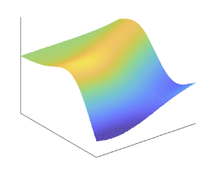
Figure 2 shows space–time surface plots of the oscillatory component of the magnetic field  $b_z^o$ (3.8), the evanescent component $b_z^e$ (3.9), the total vertical magnetic field $b_z=b_z^o+b_z^e$, and the free-surface elevation $\zeta$ (2.20), during the generation phase starting at $t=0^+$. Therefore, the full integral formulae and not the asymptotic ones are used to produce figure 2. The integrals are evaluated numerically using a Gauss–Legendre quadrature scheme. The component $b_z^o$ (figure 2a) is negative during the initial generation phase and then propagates away from the source in an oscillatory fashion. The component $b_z^e$ (figure 2b) is generated directly by the vertical motion of water pushed upwards by the seabed displacement, and hence is positive near the origin. Though $b_z^e$ is of the same order of magnitude as $b_z^o$, it decays very quickly with time, becoming negligible just after $10$ s. Therefore, $b_z^e$ is a source-specific disturbance related directly to the seabed motion.

Figure 2. Space–time surface plots of the vertical magnetic field and free-surface elevation during the generation phase: ( $a$) oscillatory component $b_z^o$ (3.8); ( $b$) evanescent component $b_z^e$ (3.9); ( $c$) total vertical field $b_z=b_z^o+b_z^e$; ( $d$) free-surface elevation (2.18). Parameters are $h=2000\ \mathrm {m}$, $A=3\ \mathrm {m}$, $\varDelta =5000\ \mathrm {m}$, $F_z=-20\,000\ \mathrm {nT}$.
As time progresses, the transient oscillatory field  $b_z^o$ is the only one that survives (figure 2c), propagating away from the source together with the tsunami (figure 2d). The asymptotic behaviour of the magnetic field at large distance from the seabed disturbance is investigated in the next subsection.
5.2. Analysis of the phase difference between gravity wave and magnetic field
Field measurements and numerical simulations have shown consistently that tsunami- generated EM signals, propagating over large distances across the ocean, exhibit a phase difference with respect to the associated tsunami (Toh et al. Reference Toh, Satake, Hamano, Fujii and Goto2011; Minami & Toh Reference Minami and Toh2013; Wang & Liu Reference Wang and Liu2013; Minami et al. Reference Minami, Toh and Tyler2015). Our novel asymptotic solution provides further physical insight into this remarkable far-field property.
Figure 3 shows the time series of the free-surface elevation  $\zeta$ (4.6) together with the oscillatory component of the magnetic field $b_z^o$ (4.13), at large distance $x=3500\ \mathrm {km}$ from the epicentre. Note the presence of a clear time lag between the EM signal and the tsunami. The first trough of the EM signal arrives at the observation point at $t\simeq 417$ min, whereas the tsunami crest arrives at $t\simeq 419\ \mathrm {min}$, i.e. after $2\ \mathrm {min}$. The tsunami period is approximately $T\simeq 9\ \mathrm {min}$, therefore the time lag between the first EM signal trough and the first tsunami crest is ${\sim }0.2\ {\rm T}$. We remark that the leading variation of the vertical magnetic field is negative. This agrees with previous studies (Minami et al. Reference Minami, Toh and Tyler2015) and is because the asymptotic magnetic field $b_z\sim b_z^{(o)}$ (4.13) depends directly on the vertical geomagnetic component $F_z$, which is negative in the example shown here.


Figure 3 shows that a clear EM signal is already present at time  $t=400\ \mathrm {min}$, where $b_z^o$ is about $15\,\%$ of its value at the first trough. This signal anticipates the arrival of the tsunami crest at the same observation point by ${\sim }19\ \mathrm {min}$. Therefore, detecting the early arrival of tsunami-generated EM signals at geomagnetic observatories has the potential to provide an advance warning of the order of tens of minutes. This represents a notable improvement on traditional tsunameter networks based on bottom pressure sensors, which are capable of only real-time detection (Levin & Nosov Reference Levin and Nosov2016).
The novel formulae of § 4 explain the reason for the time lag between the EM signal and the tsunami. At large distance from the epicentre, the vertical component of the magnetic field on the seabed is  $b_z(x,-h,t)\sim b_z^o(x,t)$ and decays as $O(t^{-1/3})$. The tsunami also decays as $O(t^{-1/3})$. Hence both the tsunami and the associated EM field exhibit the same time decay. Now note that the self-induction component $g_z^o$ (4.15) of the magnetic field depends on the Airy function, whose integrand is proportional to a cosine, and thus propagates similarly to the tsunami (4.6). On the other hand, the magnetic diffusion component $m_z^o$ (4.14) depends on the Scorer function (4.16), whose integrand is proportional to a sine. Therefore, the resulting phase lag between the Airy function in $\zeta$ and the Scorer function in $m_z^o$ is responsible for the time lag between the tsunami and the EM signal, with the latter leading the former.
A deeper physical understanding is achieved by analysing the single components of the vertical magnetic field  $b_z^o = m_z^o+g_z^o$. Figure 4 shows the time series of the magnetic field $b_z^o$ and its components $m_z^o$ (diffusion) and $g_z^o$ (self-induction) for the same parameters as in figure 3, with $h=2000\ \mathrm {m}$. Note that the diffusive component $m_z^o$ arrives earlier than the self-induction component $g_z^o$ and is dominant.

Figure 4. Time series of the magnetic field  $b_z^o$ (4.13) and its self-induction $g_z^o$ (4.15) and diffusion $m_z^o$ (4.14) components at large distance $x = 3500\ \mathrm {km}$ from the epicentre. Parameters are $h=2000\ \mathrm {m}$, $A=3\ \mathrm {m}$, $\varDelta =5000\ \mathrm {m}$, $F_z=-20\,000\ \mathrm {nT}$.
At a fundamental level, because Maxwell's equations are coupled to the liquid's velocity through Ohm's law (2.2), the lines of force of the magnetic field can move (Stern Reference Stern1966). As described by the dynamo equation (2.13), the time evolution of the magnetic field is governed by a mixture of convection by the liquid's velocity and diffusion. Now, the liquid moves at a speed close to the leading wave speed  $c_t=\sqrt {gh}\sim 140\ \mathrm {m}\ \mathrm {s}^{-1}$. On the other hand, the lateral magnetic diffusion speed is $c_d = 2\eta /h \sim 200\ \mathrm {m}\ \mathrm {s}^{-1}$ (Tyler Reference Tyler2005; Wang & Liu Reference Wang and Liu2013). Hence, the diffusive component of the vertical magnetic field travels ahead of the self-induction component and the tsunami. Physically, this explains the very early arrival of $m_z^o$ as the EM field and tsunami propagate over large distances.
We now investigate the physical picture as the water depth increases. Figure 5 shows the time series of the free-surface elevation  $\zeta$ (4.6) and the oscillatory component of the EM signal $b_z^o$ (4.13), for the same parameters as in figure 3, but with $h=4000\ \mathrm {m}$. Here, the first EM signal trough arrives at $t\sim 296\ \mathrm {min}$, whereas the first tsunami crest arrives at $t\sim 297\ \mathrm {min}$. The period is $T \sim 10\ \mathrm {min}$, therefore the time lag between the first EM signal trough and the first tsunami crest is ${\sim }0.1\ {\rm T}$. Hence increasing the water depth has the undesired effect of decreasing the time lag between the EM and the tsunami waves. This confirms previous in situ measurements and numerical modelling results (Minami et al. Reference Minami, Toh and Tyler2015).


Figure 6 shows the time series of the EM components for  $h=4000\ \mathrm {m}$. The flow speed is $c_t\sim 200\ \mathrm {m}\ \mathrm {s}^{-1}$, whereas the diffusion speed is $c_d\sim 100\ \mathrm {m}\ \mathrm {s}^{-1}$. There is no early arrival of the diffusive component, and the time lag between the EM signal and the tsunami is much reduced (see figure 5, as compared to figure 3). It is therefore clear that the ocean depth plays a major role on the EM field. In the next subsection, we investigate quantitatively the behaviour of the system with respect to the depth using our novel analytical results.

Figure 6. Time series of the magnetic field  $b_z^o$ (4.13) and its self-induction $g_z^o$ (4.15) and diffusion $m_z^o$ (4.14) components at large distance $x = 3500\ \mathrm {km}$ from the epicentre. Parameters are $h=4000\ \mathrm {m}$, $A=3\ \mathrm {m}$, $\varDelta =5000\ \mathrm {m}$, $F_z=-20\,000\ \mathrm {nT}$.
5.3. Role of ocean depth
Minami et al. (Reference Minami, Toh and Tyler2015) investigated numerically the dependence of the EM field on the ocean depth. They found that in shallow water, the process is diffusion-dominated, leading to appreciable phase lag between the EM signal and the tsunami. As the water depth increases, the phenomenon becomes self-induction-dominated, and the phase lag becomes less noticeable.
We now explain this phenomenon using our analytical solution. A qualitative understanding can be attained readily using the dynamo equation (2.13). Introduce the non-dimensional variables
 \begin{equation} \boldsymbol{u}'=\boldsymbol{u}/\sqrt{gh},\quad \boldsymbol{b}' = \boldsymbol{b}/F, \quad \boldsymbol{F}'=\boldsymbol{F}/F, \quad t'=t\sqrt{g/h},\quad (x',y')=(x,y)/h. \end{equation}
Then (2.13) becomes
 \begin{equation} \frac{\partial \boldsymbol{b}'}{\partial t'}-\frac{1}{{R_m}}\,\nabla'{^2}\boldsymbol{b}'= \boldsymbol{F}'\boldsymbol{\cdot}\boldsymbol{\nabla}'\boldsymbol{u}', \end{equation}
where  ${R_m}=h\sqrt {gh}/\eta$ is the magnetic Reynolds number. This provides an estimate of the relative importance of self-induction over diffusion. Note that ${R_m}=O(h^{3/2})$. Therefore, increasing the water depth makes the diffusive term proportional to $\nabla '{^2}\boldsymbol {b}'$ in (5.3), much smaller than the self-induction term $\partial \boldsymbol {b}'/\partial t'$: the EM dynamics is dominated by self-induction (component $g_z^o$ in (4.13)), and the time lag between gravity and EM signal decreases. On the contrary, as $h$ decreases, the magnetic Reynolds number also decreases: the dynamics is dominated by magnetic diffusion (component $m_z^o$ in (4.13)), and the time lag between gravity and EM signal increases.
This phenomenon can be further investigated quantitatively by looking at the analytical formulae (4.14)–(4.15). Since  $\mathrm {Ai}(Z)=O(\textrm{Gi}(Z))$, we have
 \begin{equation} \xi=\frac{{\rm max}\left\{ |m_z^o| \right\}}{{\rm max}\left\{ |g_z^o|\right\}}\sim \frac{2\eta}{h\sqrt{gh}}=\frac{2}{{R_m}}. \end{equation}
Expression (5.4) reveals that the ratio between the maximum diffusive component and the maximum self-induction component of the magnetic field is inversely proportional to the magnetic Reynolds number by a factor 2. For the parameters of figure 4 ( $h=2000\ \mathrm {m}$), we have $\xi = 1.54$ and $2/{R_m}=1.42$. On the other hand, for the parameters of figure 5 ( $h=4000\ \mathrm {m}$), we have $\xi = 0.54$ and $2/{R_m}=0.52$. Both cases agree well with the approximation $\xi \sim 2/{R_m}$ in (5.4). It is worth noting that a similar parameter was used by Tyler (Reference Tyler2005) and Minami et al. (Reference Minami, Toh and Tyler2015), albeit in the frequency domain. Our analysis extends the application of this parameter to transient motions in the time domain.
Figure 7 shows the way this property of the magnetic field reflects on the time lag  $\Delta t$ between the first EM signal trough and the first tsunami crest at a geomagnetic observation point. In figure 7, the non-dimensional time lag $\Delta t/\tau$ is plotted versus the magnetic Reynolds number ${R_m}$, where $\tau = \sqrt {h/g}$ is the time scale of the system. Figure 7 also shows the non-dimensional ratio $\xi$ (5.4), again plotted versus ${R_m}$. Note that both $\Delta t/\tau$ and $\xi$ do not depend on the seabed deformation parameters, but depend only on water depth and position of the observation point. Both non-dimensional parameters decrease monotonically as ${R_m}$ increases, i.e. increasing the water depth. The non-dimensional time lag $\Delta t/\tau$ almost halves by doubling the magnetic Reynolds number. Values of ${R_m}$ smaller than 1.3 correspond to a diffusion-dominated case, where $\xi >1.5$, i.e. the diffusive component $m_z^o$ is >50 % larger than the self-induction component $g_z^o$. In this regime, the Scorer term in (4.13) is more important than the Airy term, and the phase difference between the EM signal and the tsunami (which instead is proportional to Airy) results in a substantial time lag ( $\Delta t/\tau > 8$). On the other hand, ${R_m}$ values greater than 4 correspond to an induction-dominated case, where $\xi <0.5$, i.e. the self-induction component $g_z^o$ is >50 % larger than the diffusive component $m_z^o$. In this regime, the phase difference between the EM signal and the tsunami decreases significantly, leading to a reduced time lag ( $\Delta t/\tau < 3$).

Figure 7. Behaviour of the non-dimensional time lag  $\Delta t/\tau$ (dots) and the parameter $\xi$ (solid line) versus the magnetic Reynolds number ${R_m}$. The curve $y=2/{R_m}$ is plotted for reference (dashed line). The observation point is at $x=3500\ \mathrm {km}$.
In practice, the diffusion domain  ${R_m}<1.3$ corresponds approximately to $h<2000\ \mathrm {m}$. In this scenario, EM signals are precursors of the gravity wave and can provide an advance warning of the order of minutes to tens of minutes. On the other hand, the self-induction domain ${R_m}>4$ corresponds approximately to $h>4000\ \mathrm {m}$. In this case, the diffusive component is less important, and EM signals lose their potential for employment in early warning systems. We remark that our results are consistent with those obtained numerically by previous authors (e.g. see Minami et al. Reference Minami, Toh and Tyler2015) and indeed offer an analytical foundation to their models.
Our results were obtained assuming that the EM properties of the soil are insulating, following Tyler (Reference Tyler2005) and Wang & Liu (Reference Wang and Liu2013). Other studies considered a seafloor with finite electrical conductivity (Minami et al. Reference Minami, Toh and Tyler2015) or a multi-layered structure (Zhang et al. Reference Zhang, Utada, Shimizu, Baba and Maeda2014b), in which case a numerical solution is necessary. Zhang et al. (Reference Zhang, Utada, Shimizu, Baba and Maeda2014b) showed that the horizontal component of the magnetic field  $b_x$ is sensitive to the sediment layer conductivity, due to the conductive current established across the seafloor. However, the vertical component of the magnetic field $b_z$, of interest for practical applications to tsunami early warning, is less dependent on the conductivity of the seafloor. Furthermore, the conductivity of the seafloor at several observation sites in the Pacific Ocean is less than $0.1\ {\rm S}\ {\rm m}^{-1}$ and therefore can be approximated to zero (Tatehata, Ichihara & Hamano Reference Tatehata, Ichihara and Hamano2015).
In this study, we have considered a symmetric seabed deformation, for the sake of example. For a generic deformation, the forcing function  $W$ can be decomposed into symmetric and antisymmetric terms, i.e. $W(x,t) = S(x,t) + A(x,t)$, where $S(x,t) = (W(x,t)+W(-x,t))/2$ and $A(x,t) = (W(x,t)-W(-x,t))/2$. Then the EM and wave fields can be solved separately for each component, following the same steps as above, and finally summed to give the full solution.
We remark that the seabed deformation  $W(x,t)$ investigated in this paper is instantaneous. Our theory can be extended to a generic time-varying seabed deformation, say $D(x,t)$, by convolution of the instantaneous solution $b_z$ in the time domain. Hence the solution for the magnetic field, say $\hat {b}_z$, generated by $D(x,t)$, will read
 \begin{equation} \hat{b}_z(x,z,t) = \int_0^t b_z(x,z,t-\tau)\,D(x,\tau)\,\mathrm{d} \tau. \end{equation}
Physically, the latter represents the superposition of elementary impulse sources whose intensity at  $t=\tau$ is $D(x,\tau )$ (Mei et al. Reference Mei, Stiassnie and Yue2005).
The present study is limited to a two-dimensional configuration, where the disturbance on the seabed is independent of the transverse horizontal coordinate  $y$. Physically, this assumption captures well the leading-order behaviour of tsunamis generated by slender fault, whose length $L$ along $y$ is much greater than the width $w$ along $x$, i.e. $\epsilon =w/L\ll 1$. The investigation of higher-order effects $O(\epsilon )$, due to the slender fault finiteness, requires a multiple scale perturbative approach (Mei & Kadri Reference Mei and Kadri2018). If the fault is not slender, then the EM and wave fields propagate in all horizontal directions. Hence the motion is three-dimensional and a full three-dimensional theory is required. This implies solving the governing equations in polar coordinates, which is out of the scope of this paper and is envisaged for future work.
6. Conclusions
We derived a mathematical model of electromagnetic (EM) waves generated by tsunamigenic seabed deformation over an ocean of constant depth. We solved the governing dynamo equation for the EM signal, coupled with a potential flow model of Cauchy–Poisson type for the transient fluid flow forced by seabed deformation. This advances previous models where simplified formulae without direct forcing were assumed for the wave field (Wang & Liu Reference Wang and Liu2013; Minami et al. Reference Minami, Toh and Tyler2015, Reference Minami, Schnepf and Toh2021).
Using large-time asymptotics, we derived novel expressions for the magnetic field generated by an instantaneous seabed deformation. We showed that the vertical magnetic field on the seabed is made by an evanescent component  $b_z^e$, decaying at least as $O(t^{-3/2})$, and an oscillatory component $b_z^o$, decaying as $O(t^{-1/3})$, i.e. with the same rate of decay as the surface gravity wave (tsunami). The oscillatory component $b_z^o$ is in turn made of two terms: $g_z^o$ dominated by self-induction, and $m_z^o$ dominated by magnetic diffusion. Similarly to the surface gravity wave $\zeta$, the magnetic self-induction term $g_z^o$ is proportional to the Airy function, whereas the diffusive term $m_z^o$ is proportional to the Scorer function. The phase difference between the Airy and Scorer functions explains the time lag between the surface gravity wave and the EM signal observed in recent field measurements (Toh et al. Reference Toh, Satake, Hamano, Fujii and Goto2011; Lin et al. Reference Lin, Toh and Minami2021) and numerical models (Minami et al. Reference Minami, Toh and Tyler2015).
Our novel analytical solution for the magnetic field provides physical insight into the effect of water depth on the EM signal propagating away from the seabed deformation. We showed that the relative importance of the diffusive term  $m_z^o$ over the self-induction term $g_z^o$ is measured by the parameter $\xi \sim 2/{R_m}$, inversely proportional to the magnetic Reynolds number ${R_m}=h\sqrt {gh}/\eta$. For ${R_m<1.3}$ (corresponding to $h<2000\ \mathrm {m}$), the diffusive component $m_z^o$ is dominant: the EM field is a precursor of the gravity wave and can provide an advance warning of the order of minutes to tens of minutes. This is because the lateral magnetic diffusion speed is larger than the liquid's speed, hence the component of the vertical magnetic field travels ahead of the self-induction component and the tsunami.
For a typical application to tsunami early warning, the initial EM signal is  $O(0.1)$ nT; see again § 5. This signal is superimposed on the geomagnetic background noise, which is a random signal of similar magnitude (Yao et al. Reference Yao, Zhang, Teng and Yang2018). Existing seafloor EM stations are able to record scalar and vector magnetic fields with resolutions of $O(0.1)$ nT and $O(0.01)$ nT, respectively (Kawashima & Toh Reference Kawashima and Toh2016). Coherent fluctuations of the geomagnetic signal can be separated from the homogeneous background noise by means of wavelet-based filtering (Kovacs, Carbone & Vorosc Reference Kovacs, Carbone and Vorosc2001). Therefore, using EM fields to trigger TEWS is feasible with existing technology. For ${R_m}>4$ (corresponding to $h>4000\ \mathrm {m}$), the self-induction component is dominant: the time lag between the EM signal and the gravity wave decreases significantly, and the EM field loses its potential for employment in early warning systems.
Our analysis considered an idealised two-dimensional geometry with an ocean of constant depth. Future developments include the extension to three-dimensional geometry and varying depth. We also assumed that the air above the ocean and the soil below the seafloor are insulating media. A further extension of this model could consider the influence of magnetic diffusion outside the ocean.
Acknowledgements
We are grateful to H. Toh and T. Minami for their valuable suggestions on this work.
Declaration of interests
The authors report no conflict of interest.
Appendix A. Integration of (4.12)
To integrate (4.12), first expand the complex exponential inside the integrand using the Euler formula
 \begin{equation} \exp\left\lbrace \mathrm{i} \psi \right\rbrace= \cos{\psi}+\mathrm{i}\sin{\psi}, \end{equation}
where
 \begin{equation} \psi=\psi(x,k,t) = k(x-\sqrt{gh}\,t)+\frac{\sqrt{gh}}{6}\,h^2tk^3. \end{equation}
Then consider the component with  $\cos {\psi }$ and change variable
 \begin{equation} k = \left(\frac{\sqrt{gh}}{2}\,h^2t\right)^{{-}1/3}\alpha, \end{equation}
so that
 \begin{align} \int_0^\infty
\cos{\psi(x,k,t)}\,\mathrm{d} k
&=\left(\frac{\sqrt{gh}}{2}\,h^2t\right)^{{-}1/3}\int_0^\infty
\cos\left[\alpha
\left(\frac{\sqrt{gh}}{2}\,h^2t\right)^{{-}1/3}(x-\sqrt{gh}\,t)+\frac{\alpha^3}{3}
\right]\mathrm{d}\alpha \nonumber\\
&=\left(\frac{2}{\sqrt{gh}\,h^2t}
\right)^{1/3} {\rm \pi}\,\mathrm{Ai}\left[
\left(\frac{2}{\sqrt{gh}\,h^2t} \right)^{1/3} (x-\sqrt{gh}\,t)\right].
\end{align}
\begin{align} \int_0^\infty
\cos{\psi(x,k,t)}\,\mathrm{d} k
&=\left(\frac{\sqrt{gh}}{2}\,h^2t\right)^{{-}1/3}\int_0^\infty
\cos\left[\alpha
\left(\frac{\sqrt{gh}}{2}\,h^2t\right)^{{-}1/3}(x-\sqrt{gh}\,t)+\frac{\alpha^3}{3}
\right]\mathrm{d}\alpha \nonumber\\
&=\left(\frac{2}{\sqrt{gh}\,h^2t}
\right)^{1/3} {\rm \pi}\,\mathrm{Ai}\left[
\left(\frac{2}{\sqrt{gh}\,h^2t} \right)^{1/3} (x-\sqrt{gh}\,t)\right].
\end{align}
Similarly, the component with  $\sin {\psi }$ becomes
 \begin{align} \int_0^\infty
\sin{\psi(x,k,t)}\,\mathrm{d} k
&=\left(\frac{\sqrt{gh}}{2}\,h^2t\right)^{{-}1/3}\int_0^\infty
\sin\left[\alpha
\left(\frac{\sqrt{gh}}{2}\,h^2t\right)^{{-}1/3}(x-\sqrt{gh}\,t)+\frac{\alpha^3}{3}
\right]\mathrm{d}\alpha \nonumber\\
&=\left(\frac{2}{\sqrt{gh}\,h^2t}
\right)^{1/3} {\rm \pi}\,\textrm{Gi}\left[
\left(\frac{2}{\sqrt{gh}\,h^2t} \right)^{1/3} (x-\sqrt{gh}\,t)\right].
\end{align}
\begin{align} \int_0^\infty
\sin{\psi(x,k,t)}\,\mathrm{d} k
&=\left(\frac{\sqrt{gh}}{2}\,h^2t\right)^{{-}1/3}\int_0^\infty
\sin\left[\alpha
\left(\frac{\sqrt{gh}}{2}\,h^2t\right)^{{-}1/3}(x-\sqrt{gh}\,t)+\frac{\alpha^3}{3}
\right]\mathrm{d}\alpha \nonumber\\
&=\left(\frac{2}{\sqrt{gh}\,h^2t}
\right)^{1/3} {\rm \pi}\,\textrm{Gi}\left[
\left(\frac{2}{\sqrt{gh}\,h^2t} \right)^{1/3} (x-\sqrt{gh}\,t)\right].
\end{align}
Then substituting (A4)–(A5) back in (4.12) and neglecting terms  $O(k)$ and higher, which do not give a dominant contribution to the integral, yields (4.13).
Appendix B. Integration in the complex plane
Consider the inner integral in (3.1), i.e.
 \begin{equation} \mathcal{I}(k) = \frac{1}{2{\rm \pi}\mathrm{i}}\int_\varGamma \tilde{\bar{b}}_z^{(h)}({-}h;s,k)\,\mathrm{e}^{st}\,\mathrm{d} s, \quad k\in\mathbb{R},\ t>0^+, \end{equation}
where the function  $\tilde {\bar {b}}_z^{(h)}$ is given by (2.36). As described in § 3, the integrand has two purely imaginary poles at $s=\pm \mathrm {i}\omega$, and infinitely many real negative poles at $s=s_n$, $n=1,2,\dots$, given by (3.6). Let the curve $\varGamma$ in (B1) be the vertical line at $s=c$, where $c$ is a real positive number.
Figure 8 shows the complex  $s$-plane with the poles, the integration path $\varGamma$ and the branch cut introduced in § 3 to circumvent multivaluedness of $\alpha (s,k)$ (2.22). To calculate $\mathcal {I}(k)$, we close the integration path with two quarter-circles of large radius $R$,
$R$,  $C_R^+$ in $\mathrm {Im}\lbrace s \rbrace >0$ and $C_R^-$ in $\mathrm {Im}\lbrace s \rbrace <0$, together with straight lines just above and below the branch cut, plus small semicircles $C_n^{\epsilon +}$ and $C_n^{\epsilon -}$ of infinitesimal radius $\epsilon$ surrounding each pole on the negative real axis, and finally a small circle $C_\epsilon$ of radius $\epsilon$ around the branch point at $s=-k^2\eta$ (see again figure 8). The union of these contours is a closed circuit which will be denoted as $\varLambda$. It follows
 \begin{align} &\frac{1}{2{\rm \pi}\mathrm{i}}\int_{\varLambda}\tilde{\bar{b}}_z^{(h)}({-}h;s,k)\,\mathrm{e}^{st}\,\mathrm{d} s \nonumber\\ &\quad = \frac{1}{2{\rm \pi}\mathrm{i}}\left(\int_\varGamma + \int_{C_R^+} + \,{\rm{PV}}\int_{{-}R}^{{-}k^2\eta} + \sum_{n=1}^N \int_{C_n^{\epsilon +}} + \int_{C_\epsilon}\right.\nonumber\\ &\qquad \left. {}+ \mathrm{PV}\int_{{-}k^2\eta}^{{-}R} + \sum_{n=1}^N \int_{C_n^{\epsilon -}}+\int_{C_R^-}\right) \tilde{\bar{b}}_z^{(h)}({-}h;s,k)\,\mathrm{e}^{st}\,\mathrm{d} s, \quad R\rightarrow +\infty, \ \epsilon\rightarrow 0, \end{align}
where  $N$ is the total number of negative real poles $s_n$, so that $N\rightarrow +\infty$ as $R\rightarrow +\infty$, and PV is the Cauchy principal value (Mei Reference Mei1997).

Figure 8. Complex  $s$-plane with poles and branch cut.
Note that the only two poles inside  $\varLambda$ are at $s=\pm \mathrm {i} \omega$. Hence application of the residue theorem yields
 \begin{equation} \frac{1}{2{\rm \pi}\mathrm{i}}\int_{\varLambda}\tilde{\bar{b}}_z^{(h)}({-}h;s,k)\,\mathrm{e}^{st}\,\mathrm{d} s = \mathrm{Res}(-\mathrm{i}\omega) + \mathrm{Res}(\mathrm{i}\omega), \end{equation}
where
 \begin{align} &\mathrm{Res}({\pm} {\rm i}\omega)\nonumber\\ &\quad = \frac{|k|\,\tilde{H}_0(k)\,f_z^{(h)}({-}h;\pm\mathrm{i}\omega,k)\,\mathrm{e}^{{\pm}\mathrm{i}\omega t}}{\mp2\omega^2\left\lbrace 2\,|k|\,\alpha({\pm}\mathrm{i}\omega,k)\cosh\left[\alpha({\pm}\mathrm{i}\omega,k)h \right]+\left(k^2+\alpha^2({\pm}\mathrm{i}\omega,k) \right) \right. \sinh\left[\alpha({\pm}\mathrm{i}\omega,k)h \right] \rbrace} \end{align}
are the residues calculated at each pole, respectively. Let us now consider the right-hand side of (B2). Inspection of (2.36) and (2.37) reveals that  $|\tilde {\bar {b}}_z^{(h)}(-h;s,k) | = O(s^{-1})\rightarrow 0$ as $s\rightarrow \infty$ in the left half-plane. Hence by Jordan's lemma,
 \begin{equation} \int_{C_R^+{\cup} C_R^-} \tilde{\bar{b}}_z^{(h)}({-}h;s,k)\,\mathrm{e}^{st}\,\mathrm{d} s \rightarrow 0, \quad R\rightarrow +\infty. \end{equation}
Furthermore, it can be shown easily that the two principal-valued integrals on the opposite sides of the branch cut cancel each other out, i.e.
 \begin{equation} \left(\mathrm{PV}\int_{{-}R}^{{-}k^2\eta} +\mathrm{PV}\int_{{-}k^2\eta}^{{-}R}\right) \tilde{\bar{b}}_z^{(h)}({-}h;s,k)\,\mathrm{e}^{st} = 0. \end{equation}
Let us now consider the integral around the small circle  $C_\epsilon$, where $s=-k^2\eta + \epsilon \theta$, $\theta \in (-{\rm \pi},{\rm \pi} )$. As $\epsilon \rightarrow 0$, we have
 \begin{equation} \frac{1}{2{\rm \pi}\mathrm{i}} \int_{-{\rm \pi}}^{\rm \pi}\tilde{\bar{b}}_z^{(h)}(-h;-k^2\eta+\epsilon\, \mathrm{e}^{\mathrm{i}\theta})\,\epsilon\mathrm{i}\,\mathrm{e}^{\mathrm{i}\theta}\,\mathrm{d}\theta = O(\epsilon)\rightarrow 0. \end{equation}
Hence the only non-zero values on the right-hand side of (B2) are the integrals around the poles  $s_n$. Note that $\tilde {\bar {b}}_z^{(h)}$ does not change sign on the opposite pairs of semicircles $C_n^{\epsilon \pm }$. Hence application of the residue theorem yields
 \begin{equation} \sum_{n=1}^{N}\int_{C_n^{\epsilon+}\cup C_n^{\epsilon -}} \tilde{\bar{b}}_z^{(h)}({-}h;s,k)\,\mathrm{e}^{st}\,\mathrm{d} s={-} \sum_{n=1}^N \mathrm{Res}(s_n), \end{equation}
where the negative sign takes into account the direction of integration, and
 \begin{equation} \mathrm{Res}(s_n) =
\frac{|k|\,\tilde{H}_0(k)\,f_z^{(h)}({-}h;-\eta(k^2+\beta_n^2),k)}{d_n(k)}\,\mathrm{e}^{-\eta(k^2+\beta_n^2
)t} \end{equation}
\begin{equation} \mathrm{Res}(s_n) =
\frac{|k|\,\tilde{H}_0(k)\,f_z^{(h)}({-}h;-\eta(k^2+\beta_n^2),k)}{d_n(k)}\,\mathrm{e}^{-\eta(k^2+\beta_n^2
)t} \end{equation}
are the residues at the negative real poles. In (B9),  $d_n(k)$ is still given by (3.10), and the $\beta _n$ are the solutions of the magnetohydrodynamic dispersion relation (3.4).
Hence by substituting (B5)–(B9) into (B2), the integral in the complex plane (B1) simplifies to
 \begin{equation} \mathcal{I}(k) = \mathrm{Res}(-\mathrm{i}\omega) + \mathrm{Res}(\mathrm{\mathrm{i}\omega}) + \sum_{n=1}^\infty \mathrm{Res}(s_n). \end{equation}


 Open access