


1. Introduction
Turbulent flows bounded by rough walls are ubiquitous in both natural and industrial flows: examples range from river flows (Wang & Cheng Reference Wang and Cheng2006), wind flows over urban or plant canopies (Coceal & Belcher Reference Coceal and Belcher2004) to bio-fouled ship hulls (Monty et al. Reference Monty, Dogan, Hanson, Scardino, Ganapathisubramani and Hutchins2016), iced surfaces on airfoil (Gent, Dart & Cansdale Reference Gent, Dart and Cansdale2000) and fouled or corroded pipelines (Shockling, Allen & Smits Reference Shockling, Allen and Smits2006) to name a few. The estimation of the flow resistance over such rough surfaces is essential for the accurate prediction and modelling of the overall flow behaviour, yet the multitude of possible rough surfaces occurring in practice and the complex flow physics have challenged researchers for decades. Starting with the seminal work by Nikuradse (Reference Nikuradse1931) and Schlichting (Reference Schlichting1936), researchers have tried to trace back the roughness-induced friction drag to geometric characteristics of the roughness topography. A first systematic collection effort in this direction was performed by Moody (Reference Moody1944). His eponymous diagram employs characteristic roughness length scales, i.e. an equivalent sand-grain height  $k_s$, for commercially rough pipes. The values for $k_s$ are found by comparing the friction factor in the fully rough regime with the sand-grain roughness experiments by Nikuradse (Reference Nikuradse1931). However, $k_s$ is not known a priori for any new roughness topography and, when not determined directly via high-fidelity numerical or laboratory experiments, it is estimated from statistical properties of the surface topography via ever-improving empirical correlations (see Chung et al. (Reference Chung, Hutchins, Schultz and Flack2021) and Flack & Chung (Reference Flack and Chung2022), for an overview) and data-driven models (Jouybari et al. Reference Jouybari, Yuan, Brereton and Murillo2021; Lee et al. Reference Lee, Yang, Forooghi, Stroh and Bagheri2022; Yang et al. Reference Yang, Stroh, Lee, Bagheri, Frohnapfel and Forooghi2023a) derived from such experiments.
The kind of rough surfaces mostly represented in roughness databases typically feature a surface topography whose statistical properties, when computed over an area of diameter of the order of  $\delta$ (Chung et al. Reference Chung, Hutchins, Schultz and Flack2021), do not significantly vary along the surface; in other words, the rough surface is statistically homogeneous. This also implies that the surface topography varies along the directions of the surface plane with a characteristic length scale well below $\delta$. Fortunately, many rough surfaces occurring in nature and industry are statistically homogeneous over large areas; these include concrete and most steel surfaces after different processing techniques such as milling, casting, galvanisation or grit-blasting, for instance. Since any sufficiently large sample of a homogeneous rough surface (henceforth ‘statistically’ is dropped for simplicity) is representative of any bigger portion of it, the drag characteristic of homogeneous surfaces can be determined in relatively small-scale experiments, such as numerically in small or even minimal channels (Yang et al. Reference Yang, Stroh, Chung and Forooghi2022) or in the laboratory while ensuring equilibrium of the boundary layer (Flack & Schultz Reference Flack and Schultz2014) or full development of the channel or pipe flow (Flack & Schultz Reference Flack and Schultz2023).
The present knowledge of homogeneous rough surfaces is invaluable for the accurate estimation of the friction drag in several industrial applications. However, many flow scenarios are such that the statistically heterogeneous character of the rough surface cannot be neglected. While a formal or universal definition of heterogeneous roughness has not been proposed yet, for the sake of this manuscript, we consider a rough surface to be heterogeneous if the roughness statistical properties vary over a length scale which is large relative to the outer scale  $\delta$ of the flow or of similar order. This loose definition, which correctly relates the concept of roughness heterogeneity to both the surface topography and the turbulent flow, is for instance used in the review by Chung et al. (Reference Chung, Hutchins, Schultz and Flack2021). Heterogeneous rough surfaces occur, for instance, frequently in atmospheric flows, whether they be natural, such as forest canopies in mountainous areas (Schlegel et al. Reference Schlegel, Stiller, Bienert, Maas, Queck and Bernhofer2012), land-sea coastlines (Jiang et al. Reference Jiang, Wen, Sha and Chen2017) and desert dunes (Omidyeganeh & Piomelli Reference Omidyeganeh and Piomelli2013a,Reference Omidyeganeh and Piomellib), or the consequence of anthropogenic landscaping and land use, such as wind-farms (Ali et al. Reference Ali, Cortina, Hamilton, Calaf and Cal2017), patchy agricultural terrains, deforested and alternating urban areas (Hanna et al. Reference Hanna, Brown, Camelli, Chan, Coirier, Hansen, Huber, Kim and Reynolds2006). Additionally, surfaces in engineering flows may be heterogeneous on a large-scale, such as ablated turbine blades (Barros & Christensen Reference Barros and Christensen2014) or riveted rough surfaces (Suastika et al. Reference Suastika, Hakim, Nugroho, Nasirudin, Utama, Monty and Ganapathisubramani2021).
At present, little is known about the drag behaviour of heterogeneous rough surfaces and how to incorporate surface heterogeneity in predictive frameworks (Chung et al. Reference Chung, Hutchins, Schultz and Flack2021; Hutchins et al. Reference Hutchins, Ganapathisubramani, Schultz and Pullin2023). Depending on the application domain, existing models may resort to the use of  $k_s$ (Hutchins et al. Reference Hutchins, Ganapathisubramani, Schultz and Pullin2023), which can be determined and employed for full-scale predictions only in the fully rough flow regime when $C_f$ is independent of Reynolds number $Re$, or may rely on further hypotheses such as equilibrium and linearity (Bou-Zeid et al. Reference Bou-Zeid, Anderson, Katur and Mahrt2020). In either case, our current capability to predict the resistance and flow behaviour of inhomogeneous rough surfaces is limited by the lack of high-fidelity data spanning a broad range of $Re$. Such a lack of experimental evidence is best exemplified by acknowledged open questions on fundamental matters (Chung et al. Reference Chung, Hutchins, Schultz and Flack2021), such as whether certain inhomogeneous surfaces exhibit a fully rough regime or not.
The present manuscript aims at contributing with a new, systematic database of heterogeneous rough surfaces obtained via high-fidelity laboratory measurements and numerical simulations. As baseline rough surfaces, we employ commercially available sandpaper, which has a nominal average grain diameter depending on its grit size and has been frequently adopted to characterise rough-wall turbulence (Connelly, Schultz & Flack Reference Connelly, Schultz and Flack2006; Flack, Schultz & Connelly Reference Flack, Schultz and Connelly2007; Squire et al. Reference Squire, Morrill-Winter, Hutchins, Schultz, Klewicki and Marusic2016; Morrill-Winter et al. Reference Morrill-Winter, Squire, Klewicki, Hutchins, Schultz and Marusic2017; Gul & Ganapathisubramani Reference Gul and Ganapathisubramani2021; Flack & Schultz Reference Flack and Schultz2023). Due to the infinite possibilities of heterogeneous arrangements, we focus on a simplified distribution to tackle the problem and introduce the roughness heterogeneity by alternating streamwise-aligned sandpaper strips and smooth surface areas with different widths along the spanwise direction. Such spanwise periodic surfaces have been intensively investigated over the last years (Chung et al. Reference Chung, Hutchins, Schultz and Flack2021) and are known to induce turbulent secondary flows of Prandtl's second kind. While many details about the turbulent flow above surfaces with spanwise varying drag have been the focus of experimental (Hinze Reference Hinze1973; Nezu & Nakagawa Reference Nezu and Nakagawa1984; Wang & Cheng Reference Wang and Cheng2006; Wangsawijaya et al. Reference Wangsawijaya, Baidya, Chung, Marusic and Hutchins2020) and numerical (Anderson et al. Reference Anderson, Barros, Christensen and Awasthi2015; Chung, Monty & Hutchins Reference Chung, Monty and Hutchins2018; Stroh et al. Reference Stroh, Schäfer, Frohnapfel and Forooghi2020b; Neuhauser et al. Reference Neuhauser, Schäfer, Gatti and Frohnapfel2022) studies, the related global drag behaviour is largely unknown. Exceptions are streamwise aligned (smooth) ridges (see, for instance, Medjnoun, Vanderwel & Ganapathisubramani Reference Medjnoun, Vanderwel and Ganapathisubramani2020) or riblets in their drag-increasing regime, for which it was shown that a fully rough flow regime behaviour is present for a limited range of  $Re$ only (Gatti et al. Reference Gatti, von Deyn, Forooghi and Frohnapfel2020; von Deyn, Gatti & Frohnapfel Reference von Deyn, Gatti and Frohnapfel2022a). In the context of this so-called ridge-type roughness, the presence of a transitional fully rough flow regime is actually surprising since such a regime is classically associated with the pressure drag of the individual roughness elements, a flow feature that is not present for streamwise invariant ridges.
For the interpretation and generalisation of the drag behaviour of streamwise invariant ridges, it proved helpful to isolate the drag change due to surface structuring induced by turbulence from the one present under laminar flow conditions (von Deyn et al. Reference von Deyn, Gatti and Frohnapfel2022a), an approach that was also successfully employed in the context of non-spherical ducts (Jones Reference Jones1976). In the present manuscript, this strategy is extended to sandpaper roughness. The current textbook understanding (Schlichting Reference Schlichting1979) is that the drag of flows over rough surfaces remains basically unaltered under laminar flow conditions, while turbulent flows start to react to surface roughness from some Reynolds number onward. Up to this  $Re$, a surface is considered to be hydraulically smooth, i.e. the roughness is submerged in the viscous sublayer such that $k_s^+<5$. The assumption that laminar flow is unaffected by surface roughness relies on a large-scale separation between $\delta$ and the roughness height $k$. Otherwise, the friction coefficient deviates from the analytical solution for laminar smooth-wall duct flows (Huang et al. Reference Huang, Wan, Chen, Li, Mao and Zhang2013). In the context of geological flows in rock fractures, the corresponding effective channel height that reproduces the analytical relation of the smooth wall channel in the case of large surface roughness is referred to as (hydraulic) aperture (Witherspoon et al. Reference Witherspoon, Wang, Iwai and Gale1980; Brown Reference Brown1987; Berkowitz Reference Berkowitz2002).
The required scale separation for a roughness not to behave like an obstacle is typically derived from considerations under turbulent flow conditions and is stated as  $k/\delta < 1/40$ in the review by Jiménez (Reference Jiménez2004). Especially for numerical studies, large-scale separation combined with fully rough flow conditions is challenging to achieve. Therefore, many studies rely on a scale separation of $k/\delta < 1/10$, for which the rough surface may alter the flow statistics throughout a significant wall-normal portion of the flow, possibly affecting the outer-layer similarity on which most predictive frameworks for flow resistance over rough walls rely (Chung et al. Reference Chung, Hutchins, Schultz and Flack2021). The outer-layer similarity implies that rough- and smooth-wall turbulence statistics are similar sufficiently far from the wall, such that their difference can be captured solely by the roughness function $\Delta U^+$.
In the present study, we investigate laminar and turbulent channel flows over sandpaper roughness of different strip widths  $s$ with a scale separation of the order of $\delta /k = 20$. The homogeneous rough surface (representing an infinite strip width) is complemented with strip widths of the order of the full channel height, i.e. $\delta$ and $2\delta$, with equally sized smooth wall strips between them. The arrangement on the top and bottom channel wall is always symmetric around the channel centreplane. While the drag behaviour of roughness strips in the turbulent flow regime over a wide Reynolds number range is determined experimentally for the first time, direct numerical simulation (DNS) are employed to provide insights into the turbulent flow conditions at one selected $Re$ and to obtain the laminar flow solutions.
2. Investigated surface and flow configurations
The reference homogeneous rough surface, which we employ in the following for constructing both laboratory and numerical experiments of inhomogeneous roughness, is a P60 grit sandpaper. Tactile measurements (five one-dimensional line scans of  $5\ \mathrm {cm}$ length each with perthometer Mahr MarSurf PCV $^{\circledR}$) and three-dimensional reconstruction of highly resolved photographs (five surface samples of size $2\ \mathrm {cm}\times 3\ \mathrm {cm}$) using photogrammetry (Hallert Reference Hallert1960) were used to obtain the power spectrum (PS) and the probability density function (p.d.f.) of the sandpaper surface height, respectively. An initial approach to acquire two-dimensional roughness scans of P60 grit sandpaper involved using white-light interferometry measurements. This procedure was discarded due to significant surface reflections.
Note that the surface roughness height is measured for the entire thickness of the sandpaper foil, such that the base material is included in the height measurement. The corresponding roughness properties are summarised in table 1. Here  $k_{avg}$ and $k_{max}$ are the averaged and maximum height of the roughness including the base material and $k_{rms}$ is the root-mean-squared deviation of the roughness height from $k_{avg}$. Here, $Sk=1/(Sk_{{rms}}^3)\int _S(k-k_{{avg}})^3\,\mathrm {d}S$ represents skewness, $Ku=1/(Sk_{{rms}}^4)\int _S(k-k_{{avg}})^4\,\mathrm {d}S$ is kurtosis and the effective slope is defined as $ES=1/S\int _S|(\partial k)/(\partial x)|\,\mathrm {d}S$. Here, $S$ corresponds to the wall-projected surface area and $x$ is the streamwise direction. The mean roughness height $k_{avg}$ amounts to $0.67\,{\rm mm}$. The base material constitutes approximately $0.3\,{\rm mm}$ of this mean roughness height and is thus similar to the grain size of P60 sandpaper itself.
Table 1. Roughness properties of the utilised P60 sandpaper. Note that the surface height distribution is measured from the bottom of the sandpaper. Therefore, the values reported for mean roughness height  $k_{avg}$ and maximum roughness height $k_{max}$ include the base material of the sandpaper (approximately 0.3 mm). Standard deviation $k_{rms}$, skewness $Sk$, kurtosis $Ku$ and effective slope $ES$ are computed following Chung et al. (Reference Chung, Hutchins, Schultz and Flack2021).
As previously anticipated, this manuscript focuses on a particular kind of surface (and thus flow) heterogeneity, namely on spanwise heterogeneous surfaces. Spanwise heterogeneity can be achieved, for instance, via surfaces with topological variation (e.g. adjacent regions of different elevation) or surfaces with skin-friction variations (e.g. alternating regions with similar elevation but of high and low wall shear stress). In the literature (Wang & Cheng Reference Wang and Cheng2006), these two extreme cases are known as ridge-type and strip-type ‘roughness’, even when no actual rough surface is involved. Spanwise heterogeneity achieved in terms of lateral strips of different surface roughness properties, as done in the present manuscript, lies somewhat between the two extreme cases. In fact, no lateral variation of roughness properties can be achieved while keeping every possible hydraulic or geometric definition of wall elevation, some of which we will consider in the following, constant. Stroh et al. (Reference Stroh, Schäfer, Frohnapfel and Forooghi2020b) and Schäfer et al. (Reference Schäfer, Stroh, Forooghi and Frohnapfel2022) have shown that the relative elevation of the roughness strips can be a critical parameter for the related turbulent secondary flow. Therefore, we investigate three different inhomogeneous configurations in the present manuscript, as shown in figure 1. The configuration in panel (a) consists of protruding sandpaper strips alternating with equally sized portions of the smooth flat wall on which they have been glued. Clearly, in this configuration, both the roughness properties of the surface and its mean elevation vary periodically along the spanwise direction, yielding to a mixture between so-called strip- and ridge-type ‘roughness’. For the configuration in panel (c), submerged sandpaper strips aim at reproducing strip-type roughness by eliminating spanwise variations of mean elevation. Note that different hydraulic definitions of elevation may still vary along the surface. Finally, smooth ridges of height  $k_{avg}$ are used in the configuration in panel (b), resembling ridge-type roughness, to isolate the effect of pure elevation on the global drag. These configurations are complemented by the homogeneous cases of a smooth flat surface and a homogeneous rough surface completely covered with the same P60 grit sandpaper. These reference cases are necessary to determine the hydraulic properties of the homogeneous rough surface, such as its $k_s$ value.

Figure 1. Schematic representation of the investigated types of lateral inhomogeneous surface configurations. (a) Protruding sandpaper strips. (b) Smooth ridges. (c) Submerged sandpaper strips.
Table 2 provides an overview over all investigated cases along with some properties of the measured surface height distributions. The figure below the table visualises two different effective roughness height definitions. Here,  $k_{{avg}}$ corresponds to the mean thickness (meltdown height) of the sandpaper, including the base material. In the case of roughness strips (or smooth ridges), the combined meltdown height of rough (or elevated) and non-elevated smooth strips is denoted by $h_{{avg}}$. For homogeneous rough surfaces and submerged roughness strips, it holds $h_{{avg}}=k_{{avg}}$. The strip width is denoted by $s$. All rough strips or ridges are separated by smooth strips of the same width, such that the wavelength of the spanwise periodic surface structure is given by $\lambda =2s$.
Table 2. Dimensions of the experimentally investigated sandpaper configurations:  $\lambda$ measures the spanwise periodicity of the surface, $s$ is the strip width, $k_{avg}$ refers to the mean roughness height, $h_{avg}$ is the spanwise averaged meltdown height, $\delta _{avg}$ denotes the average channel half height. The ID $protruding\_rgh\_XX$ corresponds to the configuration in panel (a) of figure 1, the ID $ridge\_XX$ to the configuration in panel (b) and the ID $submerged\_rgh\_XX$ to the configuration in panel (c). Hot-wire data (§ 3.3) are available for the protruding and submerged rough strips. DNS results are available for selected cases as indicated in the DNS column.

The flow configuration employed in the present manuscript is the turbulent channel flow. The surface configurations described above are installed at both top and bottom walls of the channel. The fluid volume enclosed between the walls is similar for all investigated cases but not fully identical for the different experimental configurations. The corresponding average channel half-height  $\delta _{{avg}}$, i.e. the distance between the channel centreline and the location of $h_{{avg}}$ is used to normalise $s$ and $h_{{avg}}$ in table 2. We consider surfaces with $s/\delta _{{avg}} \approx 1$ and 2. In addition, we define the empty channel half-height as $\delta _{{empty}}=\delta _{{avg}}+h_{{avg}}$.
The choice of the channel half-height  $\delta$ is critical for the data evaluation in which the friction coefficient $C_f$ is derived from pressure drop measurements since $C_f \sim \delta ^3$ (see § 3). For rough surfaces, the channel half-height can be interpreted as the distance between the channel centre and the wall offset of the rough wall. A number of different suggestions for the wall offset $d$ can be found in the literature (Chung et al. Reference Chung, Hutchins, Schultz and Flack2021). In contrast to the geometrical quantity $d=h_{{avg}}$, other wall offset definitions are often hydraulic quantities which are evaluated based on the turbulent flow field, see e.g. Ibrahim et al. (Reference Ibrahim, Gómez-De-Segura, Chung and García-Mayoral2021). By definition, those quantities are not accessible a priori.
For ridge-type surfaces, von Deyn et al. (Reference von Deyn, Gatti and Frohnapfel2022a) show that a channel half-height derived from laminar flow conditions in the non-smooth channel is suited to isolate turbulence effects. While such a laminar reference solution can be obtained analytically for ridge-type surfaces, this is not possible for rough surfaces. At the same time, the laminar regime cannot be investigated experimentally with our facility due to the extremely low related pressure drop. Therefore, the laminar regime with rough surfaces is investigated numerically to determine one additional reference channel half-height for the present investigation (see § 5.1).
3. Experimental procedure
3.1. Experimental facility
The utilised blower tunnel facility is depicted in figure 2. The flow is driven by a radial fan and progresses through a supply pipe into a large settling chamber. The air is blown towards the back wall of the settling chamber. On the opposite side of the settling chamber, the flow is directed through a nozzle into the actual test section. The air flows through five grids embedded in wooden frames and a honeycomb flow straightener on its way through the settling chamber towards the turbulent channel flow test section. The facility allows to vary the bulk Reynolds number of the channel flow in the range of  $5\times 10^3< Re_b < 8.5 \times 10^4$ (Guettler Reference Guettler2015; von Deyn Reference von Deyn2023).

Figure 2. Schematic of the utilised wind tunnel including measurement instrumentation.
Measurements of the streamwise pressure gradient can be carried out by evaluating the static pressure at 21 pairs of pressure taps located along both side walls of a  $314\delta$ long channel test section with an aspect ratio of 1 : 12. The channel test section is divided into three segments of $76\delta$, $119\delta$ and $119\delta$ streamwise extent. As in previous investigations with the same facility (Gatti et al. Reference Gatti, Güttler, Frohnapfel and Tropea2015, Reference Gatti, von Deyn, Forooghi and Frohnapfel2020; von Deyn et al. Reference von Deyn, Gatti, Frohnapfel and Stroh2021, Reference von Deyn, Gatti and Frohnapfel2022a), the flow is tripped at the inlet of the first segment.
In the present investigation, the last segment is equipped with sandpaper (strips) or smooth ridges symmetrically arranged on the upper and lower sides of the test section. The protruding smooth ridges of the configuration in figure 1(b) are realised by notches of depth  $k_{{avg}}$ milled in aluminium plates with a high-precision milling machine. The submerged configuration in figure 1(c) is obtained by gluing the sandpaper strips into these notches. In the case of the configuration in figure 1(a), the sandpaper strips are glued on top of the smooth channel such that the protrusion corresponds to the entire thickness of the sandpaper, including the base material, as described in the last section. In the case of homogeneous roughness (sandpaper on both channel walls), the sandpaper is glued on top of the smooth channel walls. The resulting average channel half-heights $\delta _{{avg}}$ are provided in table 2.
3.2. Skin-friction measurements
As we are going to illustrate, the present facility allows to measure the time-averaged streamwise pressure gradient  $\varPi$ and the volumetric flow rate $\dot {V}$ per unit channel depth very accurately. The average skin-friction is going to be determined from these two measured quantities. For statistically two-dimensional and fully developed turbulent channel flow with smooth walls, the wall-shear stress $\tau _w$ depends on $\varPi$ through
 \begin{equation} \tau_w=-\varPi \delta, \end{equation}
where  $\delta$ corresponds to the channel half-height (whichever specific definition is chosen). Equation (3.1) is used to deduce the skin-friction coefficient
 \begin{equation} C_f=\frac{2 \tau_w}{\rho U_b^2}, \end{equation}
where  $\rho$ is fluid density and $U_b=\dot {V}/(2 \delta )$ is the bulk velocity, also used for the formulation of the bulk Reynolds number
 \begin{equation} Re_b=\frac{2\delta U_b}{\nu}=\frac{\dot{V}}{\nu} \end{equation}
with kinematic viscosity  $\nu$ and $\dot {V}$ volume flow rate per unit channel depth. Additionally, based on $\tau _w$, the friction velocity $u_\tau =\sqrt {{\tau _w}/{\rho }}$ and the respective friction Reynolds number $Re_\tau ={u_\tau \delta }/{\nu }$ are obtained.
Equation (3.1) is derived for turbulent channels with plane walls, for which  $\tau _w$ represents the temporally and spatially averaged wall-shear stress and $\delta$ the univocally defined channel half-height. When the same equation is applied to non-planar surfaces, $\tau _w$ is replaced by an effective wall-shear stress $\tau _{w,{eff}}$, which balances the measured pressure gradient as if it was caused by a virtual flat wall placed at distance $\delta$ from the channel centre. Since $\varPi$ and $\dot {V}$ are measured in the experiment, $Re_b$ does not depend on the choice of $\delta$. However, with $U_b = \dot {V}/ 2\delta$, we obtain $C_f \sim \delta ^3$, so that different definition of $\delta$ yields different values of $\tau _w$, $U_b$ and $C_f$ for measured values of $\varPi$ and $\dot {V}$. Different choices of $\delta$ will be discussed in § 5.1.
The volume flow rate  $\dot {V}$ is measured with an orifice flow meter on the suction side of the wind tunnel (see figure 2). The orifice pressure drop is measured with one of two Setra 239D (125 and 625 Pa full-scale) unidirectional differential pressure transducers with an accuracy of 0.07 % of the full-scale, switching automatically depending on $Re_b$. For the sake of covering a range of bulk Reynolds numbers of $4.5 \times 10^3 < Re_b <8.5 \times 10^4$ in the test section, two different orifice flow meters are installed with inlet-pipe diameters of $D_o = 100$ mm and $D_o =200$ mm, respectively. Each custom manufactured annular orifice measuring chamber can be equipped with orifice plates of varying inner diameter $D_i$. The configurations are specified in table 3.
Table 3. Specifications of the different orifice flow meter configurations. The size of the markers used in figures 6, 8, 9 and 10 indicates orifice flow meter employed for the respective measurement.


Figure 6.  $C_f$ versus $Re_b$ for smooth and homogeneous rough surfaces. The experimental (Exp) rough wall data are evaluated based on three different channel half-height definitions ( $\delta =\{\delta _{{empty}}, \delta _{{avg}}, \delta _{{lam}}\}$). The different symbol sizes correspond to different flow rate measurements as specified in table 3. The complementary DNS results based on a wall shear stress evaluation at a wall offset $d=\{0, h_{{avg}},h_{{lam}},h_{\mathrm {Jackson}}\}$, yielding the respective definitions of $\delta$, are included. The correlation proposed by Dean (Reference Dean1978) for turbulent duct flows of large aspect ratio is shown as a black line.
The time-averaged streamwise pressure gradient  $\varPi$ along the test section (i.e. the last segment of the channel) is evaluated based on seven pairs of $0.3\,mm$ diameter static pressure taps spaced 200 mm in the streamwise direction along the channel in this region. Measurements are carried out with an MKS Baratron 698A unidirectional differential pressure transducer with 1333 Pa maximum range and an accuracy of 0.13 % of the reading. An eighth pair of pressure taps, located close to the test section exit, is discarded due to visible outflow effects.
Classically, one would aim to evaluate  $\varPi$ based on data far downstream of the transition location from smooth to rough surface to ensure fully developed flow conditions. At the same time, the pressure difference between two consecutive measurement locations is very small such that an evaluation of the pressure gradient over a larger streamwise distance enables higher measurement accuracy. Therefore, the pressure gradient over the entire test section was analysed carefully. Interestingly, the pressure measurements do not reveal a significant development length for the pressure gradient after the streamwise change from smooth to rough surface conditions. Based on this observation, we decided to base the evaluation of $\varPi$ on seven pressure measurement locations in the rough channel, where the first pressure measurement location is located only $8\delta$ downstream of the transition from smooth to rough surfaces. A cross-check with data evaluation based on pressure taps located further downstream only, reveals relative differences in $\varPi$ below $1.6\,\%$.
Changes in ambient conditions are accounted for by tracking the systems inlet and outlet temperature via PT100 thermocouples, and the ambient pressure and humidity using Adafruit BMP 388 and BME 280 sensors, respectively. Details of this procedure are described by von Deyn (Reference von Deyn2023).
Based on  $\varPi$ and $\dot {V}$, the skin-friction coefficient $C_f$ defined through (3.2) can be deduced. The changes in skin-friction drag $\Delta C_f=C_f-C_{f0}$ are obtained by comparing two consecutive experiments: first a smooth wall measurement used as a common reference for all structured cases was conducted to obtain $C_{f0}$ followed by skin-friction measurements of the structured plates. The smooth data are fitted with a polynomial function of fifth order for each orifice configuration stated in table 3 enabling a comparison at constant flow rate between smooth and structured cases. All measurements are carried out in the most downstream third 1500 mm (or $119\delta$) portion of the test section. The pressure taps in the second segment are used as a reference to confirm reproducibility between different measurements.
3.3. Velocity measurements
A hot-wire probe is used to measure the streamwise velocity at different wall-normal and spanwise positions. The streamwise location of the measurement campaign was fixed to one centimetre upstream of the test section outlet, since measurements showed that first- and second-order statistics were identical to those measured further upstream up to 15 cm upstream of the test section outlet. The probe consists of a single hot-wire and is of boundary-layer type (replicating a DANTEC 55P15) with a  $2.5\ \mathrm {\mu }$m diameter platinum wire and a sensing length of approximately 0.5 mm, resulting in an inner-scaled wire length of $L^+\approx 20$ at a friction Reynolds number of $Re_\tau ={u_\tau \delta }/{\nu }\approx 550$.
A DANTEC Streamline Pro frame in conjunction with a 90C10 constant temperature anemometer (CTA) system is used and operated at a fixed overheat ratio of 80 %. The velocity calibrations for the hot wires were performed ex situ in an external high contraction ratio jet facility, while mean temperature changes during the runs were limited to  ${<}2$ K and could therefore be compensated as outlined by Örlü & Vinuesa (Reference Örlü and Vinuesa2017). Turbulence statistics were acquired with a sampling time between 10 and 60 s and an acquisition frequency of 60 kHz, depending on $Re_b$. An offset and gain was applied to the top of the bridge voltage to match the voltage range of the 16-bit A/D converter used. To avoid aliasing at the higher velocities, an in-built analogue low-pass filter was set up at the Nyquist frequency prior to data acquisition.
The HWA measurements were conducted with an automated traversing system. Two-dimensional scans consisting of 870 measurement points in the spanwise and wall-normal direction were carried out ( $z$–
$z$– $y$-plane). The $30$ measurement points in spanwise direction were spaced equidistantly above the rough and smooth surface parts and refined at the sandpaper strip edges, while $29$ wall-normal locations were spaced logarithmically.
4. Numerical procedure
DNS is employed to obtain flow solutions for selected rough surfaces in the laminar and in the turbulent flow regime. The numerical representation of the rough surface is realised through the immersed boundary method (IBM) following Goldstein, Handler & Sirovich (Reference Goldstein, Handler and Sirovich1993). The code is previously validated and employed by e.g. Forooghi et al. (Reference Forooghi, Stroh, Magagnato, Jakirlić and Frohnapfel2017). The Navier–Stokes equation writes
 $$\begin{gather} \boldsymbol{\nabla}\boldsymbol{\cdot} \boldsymbol{u}=0, \end{gather}$$
 $$\begin{gather}\frac{\partial \boldsymbol{u}}{\partial t}+\boldsymbol{\nabla}\boldsymbol{\cdot}(\boldsymbol{uu})=-\frac{1}{\rho}\boldsymbol{\nabla} p+\nu\nabla^2\boldsymbol{u}-\frac{1}{\rho}\varPi{\boldsymbol{e_x}}+\boldsymbol{f}_{\!\!IBM}, \end{gather}$$
where  $\boldsymbol {u}=(u,v,w)^\intercal$ is the velocity vector and $\varPi$ is the time-averaged pressure gradient in the flow direction to drive the flow. Moreover, $p$,
$p$,  $\boldsymbol {e_x}$, $\rho$, $\nu$ and $\boldsymbol {f}_{\!\!IBM}$ denote pressure fluctuation, streamwise unit vector, density, kinematic viscosity and external body force term due to IBM, respectively. DNS is carried out in plane channel flow, in which the flow is driven by a pressure gradient at a constant flow rate (CFR). The roughness structures are installed on both the upper wall and lower wall. Periodic boundary conditions are applied in the streamwise and spanwise directions. In contrast to the experiment, the DNS is thus statistically two-dimensional without side walls. A representation of the simulation domain of size $L_x\times L_y\times L_z$ with walls covered by homogeneous roughness is shown in figure 3. In this paper, $x, y, z$ denote the streamwise, wall-normal and spanwise direction, respectively.

Figure 3. Schematic representation of the simulation domain with homogeneous sandpaper roughness. In analogy to the experiment, the sandpaper is placed on top of the smooth channel, such that also the base material of the sandpaper is modelled by the IBM.
The key challenge for the numerical simulations in the present study is to prescribe matching surface boundary conditions with the experiment attributed to the uncertainty arising from surface measurement. This was overcome through artificially generating a rough surface that reproduces the measured p.d.f. and PS of the sandpaper from respective accurate approaches while preserving its stochastic nature based on the algorithm by Pérez-Ràfols & Almqvist (Reference Pérez-Ràfols and Almqvist2019). Yang et al. (Reference Yang, Velandia, Bansmer, Stroh and Forooghi2023b) used this roughness reconstruction method to reproduce ‘digital’ realistic roughness scans, with DNS-based evaluations of  $k_s$ being consistent over different realisations of reproduced surfaces. As will be shown in § 5.2, this surface reconstruction method based on PS and p.d.f. obtained through perthometer and photogrammetry measurements as described in § 2 yields DNS-based results for $C_f$ which are in very good agreement with the presented experimental data in turbulent flow, signifying the successful reproduction of realistic sandpaper flow properties through the current procedure.
Laminar simulations are carried out at  $Re_b=133$ for all roughness strips and for the homogeneous rough reference case. The corresponding domain size and computational grid points are summarised in table 4. In the simulations of roughness strips, two roughness strips are accommodated in the simulation domain. Thus, for the wide strip configurations with $s\approx 2 \delta$, the spanwise domain size $L_z$ and grid points $N_z$ are correspondingly doubled, such that the resolution of DNS remains unchanged. The topography of the roughness strips are cropped from the aforementioned artificial sandpaper roughness. To investigate potential Reynolds number effects, additional simulations at $Re_b=13$ and $Re_b=1333$ are carried out for the case with homogeneous surface roughness.
Table 4. DNS case overview of laminar configurations. Here  $\delta$ corresponds to the empty channel half-height $\delta _{{empty}}$.

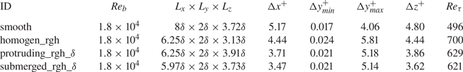
Turbulent channel flow simulations are carried out at  $Re_b=1.8 \times 10^4$ for the smooth, homogeneous rough and selected rough strip cases, namely the $s\approx \delta$ cases. The related domain size and resolution are summarised in table 5.
Table 5. DNS case overview of turbulent flow configurations. Here  $\delta$ corresponds to the empty channel half-height $\delta _{{empty}}$.
The effective wall shear stress (and thus  $u_\tau$) is obtained by extrapolating the (linear) total shear stress profile to the wall location. This wall location is defined by the choice of the wall offset $d$ which corresponds to the y-location in the computational box located at distance $\delta$ from the channel centre. The minimum value of $d=0$ and thus the largest $\tau _{w,{eff}}$ corresponds to the choice of $\delta =\delta _{{empty}}$. The non-dimensionalisation of the grid resolution (in plus units) in table 5 is based on this choice, as it results in the largest values for $u_\tau$. The resulting $Re_\tau$ is also included. The corresponding bulk velocity $U_b$ is obtained based on the spatial integration of the time-averaged velocity profile which is consecutively normalised by the domain width and the chosen channel height. Once $U_b$ is defined, $C_f$ can be evaluated following (3.2). The related results are shown in figures 6 and 8.
The values of  $\Delta U^+$ reported in figures 7 and 9 are obtained by averaging the mean velocity offset in the region $(\kern -0.01em y-d)^+=80\unicode{x2013}250$. In the case of the rough strips, the mean velocity profile is based on a spanwise average over the entire computational box. The resulting global mean velocity profiles exhibit a well defined logarithmic region that allow for extracting a roughness function based on the described approach which is in agreement with the findings of Castro et al. (Reference Castro, Kim, Stroh and Lim2021) for turbulent flow over streamwise aligned rectangular ridges.

Figure 7. Roughness function  $\Delta U^+$ against the (a) mean roughness height $h_{avg}$ and (b) the equivalent sand grain roughness height $k_s^+$. Symbols as in figure 6. The additional dotted line shows in panel (a) the logarithmic relationship $\Delta U^+=({1}/{\kappa })\ln {h_{avg}^+}+C$ with an arbitrary constant $C=-3.3$ and in panel (b) the fully rough law $\Delta U^+=({1}/{\kappa })\ln {k_{s}^+}-3.5$. In both cases $\kappa =0.39$.

Figure 8. (a) Skin-friction coefficient  $C_f$ and (b) relative drag increase $\Delta C_f/C_{f,0}$ as a function of $Re_b$ based on $\delta =\delta _{{lam}}$. Legend of panel (a) also valid for panel (b). Panel (b) also includes the limit of very wide submerged roughness strips, see (5.4a–c), as dashed black line.
Note that a low-pass filter was applied to the generated rough surface (for both homogeneous roughness and roughness strips) at a wavelength that corresponds to  $\lambda _{min}=0.6$ mm in physical size. This ensures that the smallest in-plane roughness wavelength is represented by approximately eight grid points for the homogen_rgh, the spacing of which corresponds to $\varDelta _x=\varDelta _z=0.08$ mm. It is worth noting that the grid point spacing for protruding_rgh_ $\delta$ and submerged_rgh_ $\delta$ are finer (see table 5). While the ratio $\lambda _{min}/\Delta x\approx 8$ is slightly smaller than what is suggested by Busse, Lützner & Sandham (Reference Busse, Lützner and Sandham2015), it was found to be sufficient in previous work (Yang et al. Reference Yang, Stroh, Chung and Forooghi2022) with the same numerical code.
5. Drag behaviour
5.1. Laminar drag in rough wall channel flow
In a smooth wall channel, it holds that  $C_f=12/Re_b$ for laminar flow conditions. Figure 4 shows the DNS data of the homogeneous rough surface in comparison with this reference at three different $Re_b$. The data evaluation for $C_f$ is carried out in different ways. First, $\tau _{w,{eff}}$ is obtained by extrapolating the linear shear stress profile found above the roughness to $d=0$ (blue crosses). The obtained results represent the total flow resistance introduced by the sandpaper and can thus be reproduced through an integration of $\boldsymbol {f}_{\!\!IBM}$ in the computational domain (grey squares). These results correspond to choosing the empty channel half-height $\delta _{{empty}}$ as reference. Second, $\tau _{w,{eff}}$ is evaluated by extrapolating the linear shear stress profile to $d=h_{{avg}}$ (red circles) which corresponds to a reference channel half-height of $\delta _{{avg}}$. This is identical to an evaluation of $\tau _{w,{eff}}$ based on the streamwise pressure gradient $\varPi$ and $\delta _{{avg}}$ according to (3.1) (black stars). The obtained value corresponds to the total drag (force) transferred from the fluid to the channel walls per unit planar surface area. While $Re_b$ is independent from the choice of $\delta$, $U_b$ is required to compute $C_f$. As introduced in § 3.2, we define $U_b = \dot {V}/ 2\delta$ such that $U_b$ depends on the choice of $\delta$.

Figure 4. The product  $Re_bC_f$ as a function of $Re_b$ for homogeneous rough reference DNS in the laminar regime. The effective wall shear stress is either evaluated at $d=0$ or $d=h_{{avg}}$.
In figure 4, the results based on  $d=h_{{avg}}$ are slightly above $Re_b C_f =12$, while the results based on $d=0$ result in significantly larger values for the product $Re_b C_f$ as expected. The results demonstrate that the sandpaper increases the friction coefficient of the laminar flow in the present set-up and that the degree of this increase depends (weakly) on $Re_b$ and on the choice of the reference channel half-height. We note that close observation of the original results of Nikuradse in e.g. Schlichting (Reference Schlichting1979) indicates a similar tendency; i.e. all measured data points are located slightly above the smooth wall reference. While not explicitly stated in the literature, we assume (based on the available information) that the empty pipe diameter (i.e. the inner pipe diameter measured before tightly covering the inside with sand grains of uniform size) was used in this data evaluation.
One can define an effective channel half-height for the sandpaper case which fully recovers the smooth wall laminar flow relation  $C_f=12/Re_b$. This quantity is termed laminar reference channel half-height $\delta _{{lam}}$ in the following. It represents the half-height of a smooth channel that reproduces the pressure drop–flow rate relation of the rough channel at the considered Reynolds number and is given by
 \begin{equation} \delta_{{lam}} =\delta \sqrt[3]{\frac{C_{f,0}}{C_f}} =\sqrt[3]{\frac{3\rho \nu }{2} \frac{\dot{V}}{|\varPi|}}.\end{equation}
Here,  $\delta$ corresponds to the channel half-height employed to evaluate $C_f$ of the rough channel, while $C_{f,0}$ is the smooth wall friction coefficient at the same $Re_b$. The relation $\delta _{{lam}}=\delta _{{empty}}-h_{{lam}}$ introduces $h_{{lam}}$ as a further possible choice for the wall offset $d$ that the flow perceives. We note that the hydraulic quantity $\delta _{{lam}}$ is similar to the hydraulic fracture aperture used to describe geological flows in fractured rocks (Berkowitz Reference Berkowitz2002; Cheng et al. Reference Cheng, Hale, Milsch and Blum2020).
The same reference channel half-height definition was previously employed successfully in the context of riblets and ridges (von Deyn et al. Reference von Deyn, Gatti and Frohnapfel2022a). Ridge type surfaces are invariant in the streamwise direction so that the dimensionless Stokes solution for parallel flows is exactly valid in the entire laminar regime and thus no Reynolds number dependency of  $\delta _{{lam}}/\delta _{{avg}}$ is present. The flow over rough surfaces is not exactly parallel in the very vicinity of the wall and therefore the ratio $\delta _{{lam}}/\delta _{{avg}}$ is expected to be slightly $Re$-dependent. This effect is visible in figure 5 where larger values of $\delta _{{lam}}/\delta _{{avg}}$ are found for lower Reynolds number. The ratio is generally slightly smaller than one indicating that the drag on individual roughness elements leads to a larger effective blocking of the channel cross-section than the corresponding meltdown height for the present surface. This effective blocking increases with Reynolds number indicating a Reynolds number dependent drag contribution of the roughness elements that differs from pure viscous drag. However, this effect is small and the variation of $\delta _{{lam}}$ with $Re_b$ remains within less than $0.5\,\%$ (of the smallest $\delta _{{lam}}$, i.e. the one at $Re_{b}=1333$) over the considered Reynolds number range. In the following, we consider $\delta _{{lam}}$ evaluated at $Re_{b}=133$ as the laminar reference height.

Figure 5. Reynolds number dependence of  $\delta _{{lam}}/\delta _{{avg}}$ derived from DNS for the case homogen_rgh.
The obtained ratios for  $\delta _{{lam}}/\delta _{{avg}}$ for all different surfaces considered in the present work are summarised in table 6 along with $\delta _{{empty}}/\delta _{{avg}}$. While $\delta _{{lam}}$ is very similar to $\delta _{{avg}}$ in all cases, the deviation of $\delta _{{empty}}$ is of the order of a few percent. Despite the relatively small nominal differences for different channel height definitions, the choice of channel height has a non-negligible impact on the evaluation of $C_f$ from the measured quantities of the experiment. To demonstrate the sensitivity of $C_f$ towards the channel height definition, $\delta _{{empty}}$, $\delta _{{avg}}$ and $\delta _{{lam}}$ are employed as reference channel half-heights to evaluate the friction coefficient for the homogeneous sandpaper roughness in the turbulent flow regime in the next section.
Table 6. Different channel half-height definitions in comparison to  $\delta _{{avg}}$.

5.2. Turbulent drag of homogeneous sandpaper roughness
Figure 6 shows the drag curves, derived from the pressure drop and flow rate measurements, based on the three different choices of reference channel half-height in comparison to the smooth wall data. As expected due to their similarity,  $\delta _{{avg}}$ and $\delta _{{lam}}$ yield similar results, while $\delta _{{empty}}$ yields significantly higher $C_f$-values. All drag curves do not collapse with the smooth wall reference within the investigated Reynolds number range, i.e. do not indicate a hydraulically smooth behaviour for $Re_b > 4500$. In the present case, a fully rough regime is found from approximately $Re_b=40\,000$ onward after which the relative increase in $C_f$ is less than $1.5\,\%$ up to the highest measured Reynolds number for the homogeneous rough surface ( $Re_b\approx 66\,400$). In agreement with the results of Flack & Schultz (Reference Flack and Schultz2023), the $C_f$ of the fully rough regime for sandpaper is approached from lower $C_f$-values, thus reproducing the transitionally rough drag behaviour reported by Nikuradse (Reference Nikuradse1931), which differs form the corresponding drag regime of the Moody diagram (Moody Reference Moody1944).
The DNS data which are available for  $Re_b=1.8 \times 10^4$ are also included in figure 6 and evaluated based on $\delta _{{empty}}$, $\delta _{{avg}}$ and $\delta _{{lam}}$. For the DNS data, this implies that the wall shear stress is determined at a wall offset of $d=0$, $d=h_{{avg}}$ or $d=h_{{lam}}$. All numerical data points are in very good agreement with the experimental data. To our knowledge, this is the first direct comparison of a rough surface friction coefficient derived from experimental and numerical data for statistically identical rough surfaces. The obtained agreement provides a valuable cross-validation of the two methods and further supports the conclusion of Yang et al. (Reference Yang, Stroh, Chung and Forooghi2022, Reference Yang, Velandia, Bansmer, Stroh and Forooghi2023b) that the p.d.f. and PS of the surface height distribution contain the relevant information required to reproduce the global friction behaviour of a homogeneous rough surface. Only the smooth wall DNS data point is slightly below the experimentally obtained $C_{f,0}$, in agreement with classical literature data (Kim, Moin & Moser Reference Kim, Moin and Moser1987). This difference reflects the drag contribution of the duct side walls. The improved agreement between DNS and experimental data for the rough surfaces can be explained by the smaller relative contribution of the (smooth) side wall to the total friction drag when the main duct walls are rough.
For rough wall DNS data, different definitions of the wall offset  $d$ (also sometimes referred to as virtual origin) and thus the resulting channel height can be found in the literature (Chung et al. Reference Chung, Hutchins, Schultz and Flack2021). Those often rely on flow field information which is not accessible in experiments and is generally not known a priori. We note that the method proposed by Jackson (Reference Jackson1981), in which the wall offset is evaluated based on a torque balance of the drag force profile on the roughness elements, yields very close agreement with $d=h_{{lam}}$ in terms of the computed $C_f$ for the present data set. A corresponding data point is also added in figure 6. Following the procedure described by Gatti et al. (Reference Gatti, von Deyn, Forooghi and Frohnapfel2020), the difference in skin friction coefficient between the rough ( $C_f$) and the smooth ( $C_{f,0}$) surface at the same $Re_b$ can be translated into an estimate of the roughness function $\Delta U^+$ via
 \begin{equation} \Delta U^+=\frac{1}{\kappa} \ln{\sqrt{\frac{C_f}{C_{f,0}}}}+ \sqrt{\frac{2}{C_{f,0}}}-\sqrt{\frac{2}{C_{f}}}\end{equation}
with  $\kappa =0.39$. The corresponding results are shown in figure 7(a). In this figure, $\Delta U^+$ is plotted versus $h^+_{{avg}}$. The latter is chosen as a parameter for this plot since $h_{{avg}}$ is a geometrical surface quantity (in contrast to the hydraulic nature of $h_{{lam}}$) which coincides with $k_{{avg}}$ for the homogeneous sandpaper roughness. The black dotted line in the plot is an arbitrary reference to indicate the slope $1/\kappa$ in the semi-logarithmic plot which holds for fully rough flow conditions. In agreement with the data shown in figure 6, the roughness function is significantly higher if the data evaluation is based on $h_{{empty}}$.
In addition to the experimental data, figure 7(a) also contains the DNS data, for which  $\Delta U^+$ is obtained from the velocity profile in its logarithmic region by comparison with a smooth wall reference flow at the same $Re_b$. Hereby $d$ is employed as wall offset and as evaluation location for $\tau _w$. For $d=h_{{lam}}$, this procedure yields $\Delta U^+=6.18$, while the application of (5.2) to the DNS data yields $\Delta U^+=6.12$ (not shown in the figure), showing that the two approaches are compatible and yield the same results when applied on the same data. The visible difference between $\Delta U^+$ extracted from DNS and from experiments is thus not related to the different means of retrieving $\Delta U^+$ but stems from the difference in $C_{f,0}$ for experiments and simulations owing to the finite channel width in the experiment.
In figure 7(b), the data are shifted horizontally until an agreement with the fully rough reference of Nikuradse (Reference Nikuradse1931),
 \begin{equation} \Delta U^+=\frac{1}{\kappa}\ln{k_{s}^+}-3.5 \end{equation}
with  $\kappa =0.39$ obtained for large values of $\Delta U^+$. This shift allows to deduce a value for the equivalent sand grain height $k_s$ (Chung et al. Reference Chung, Hutchins, Schultz and Flack2021). For the present homogeneous rough surface of P60 sandpaper and $d=h_{{lam}}$, a collapse with the fully rough reference is obtained for $\Delta U^+>7.5$. The equivalent sand grain roughness height is evaluated to $k_{s}=0.72\,{\rm mm}$ and is thus in reasonable agreement with $k_s \approx 0.6\,{\rm mm}$ that can be estimated based on the data published by Gul & Ganapathisubramani (Reference Gul and Ganapathisubramani2021) for P60 sandpaper with drag balance measurements in a turbulent boundary layer in the transitionally rough regime (cf. table 2 of Gul & Ganapathisubramani Reference Gul and Ganapathisubramani2021). The obtained result is also in agreement with the observation by Flack & Schultz (Reference Flack and Schultz2023) that sandpaper exhibits an equivalent sand grain roughness height approximately 2 to 2.5 times larger than its grit size (approximately 0.26 mm for P60).
However,  $k_s$ is sensitive to the channel half-height definition (or in other words, the chosen wall offset $d$). Based on $\delta _{{empty}}$ ( $d=0$), we find $k_{s,{empty}}=1.20\,{\rm mm}$, while $\delta _{{avg}}$ ( $d=h_{{avg}}$) yields $k_{s,{avg}}=0.78\,{\rm mm}$ for an average roughness height of $k_{{avg}}=0.67\,{\rm mm}$. The significantly higher value obtained for the empty channel reference half-height reflects the fact that the base material of the sandpaper is considered as part of the surface roughness in this case and the related blockage is thus translated into a contribution of the equivalent sand grain height. The observation by Volino & Schultz (Reference Volino and Schultz2022) that $k_s$ was found to vary noticeably and inversely with the turbulent boundary layer thickness $\delta _{BL}$ for $\delta _{BL}/k_s \lessapprox 40$ might be related to a similar effect. For the present data, it holds that $\delta _{empty}/k_{s,{empty}} \approx 11$ and $\delta _{lam}/k_{s} \approx 17$.
Flack & Schultz (Reference Flack and Schultz2023) report an earlier onset of fully rough conditions for sand grain roughness compared with the Nikuradse data ( $k_{s,r}^+=45$ instead of $k_{s,r}^+=70$) as documented by Schlichting (Reference Schlichting1979). The present data do not confirm this finding but indicate an onset of the fully rough regime at $k_{s,r}^+\approx 80$ which is in reasonable agreement with the classical literature data. In case of data evaluation based on $\delta _{empty}$, this value is shifted to $k_{s,r,{empty}}^+=130$.
In conclusion, we consider  $\delta _{{empty}}$ not to be an appropriate choice of channel half-height in the case of relatively large $k/\delta$ as in the present experiments. The following data evaluation is based on $\delta _{{lam}}$, since we will eventually compare this quantity with an analogous definition under turbulent flow conditions. The additional data evaluation for $C_f$ based on $\delta _{{avg}}$ and $\delta _{{empty}}$ is provided in the Appendix. We note that data evaluation based on $\delta _{{avg}}$ yields very similar results to those with $\delta _{{lam}}$ while being a geometrical and not a hydraulic property of the surface. To which extent this similarity holds for other random rough surfaces remains to be investigated.
5.3. Turbulent drag of sandpaper strips
After having characterised in detail the properties of the flow over homogeneous sandpaper roughness in the previous section, we now discuss the inhomogeneous roughness cases. The skin friction coefficient as a function of Reynolds number is shown for the investigated roughness strips in linear scaling in figure 8(a), where the data evaluation is based on  $h_{{lam}}$, while the corresponding results based on $h_{{avg}}$ and $h_{{empty}}$ are presented in the Appendix. Figure 8 contains data for four different roughness strips: one pair of protruding strips (plotted in shades of red) and one of submerged strips (plotted in shades of yellow). Each pair consists of strips of $s\approx \delta$ (dark colour) and $s\approx 2\delta$ (light colour), respectively. The data for smooth ridges (plotted in shades of blue) with both $s-$values are included in dark and light blue together with smooth and homogeneous rough references. The local minimum of $C_f$ for the homogeneous rough surface, as found in the original Nikuradse data and as reported by Flack & Schultz (Reference Flack and Schultz2023) for sandpaper, can be observed in this representation. The rough strips also exhibit a local minimum of $C_f$ in the low-Reynolds-number range, whereas the smooth ridges show $C_f$ monotonically decreasing with $Re_b$.
It can be clearly seen that all roughness strips do not reach a Reynolds number independent  $C_f$ (and thus a fully rough flow state) in the high-Reynolds-number range of the experimental facility. However, there appears to be a plateau of constant $C_f$ over some Reynolds number range around $20\,000 < Re_b < 40\,000$. This plateau corresponds the maximum $C_f$ for each strip type. While the two types of strips (protruding and submerged) with $s\approx 2\delta$ (light colour) basically show identical drag behaviour, the strips with $s\approx \delta$ (dark colour) differ in this respect, with the protruding strips resulting in larger $C_f$.
The present DNS results for protruding and submerged sandpaper strips with  $s\approx \delta$ are also included in figure 8(a). As for the homogeneous rough case, very good agreement between DNS and experimental results is obtained for these rough strips. The DNS results replicate the slightly higher drag coefficient for the protruding strips compared with the submerged counterpart with $s \approx \delta$.
Larger drag coefficients for protruding roughness strips were also reported for roughness strips with  $s\approx \delta /2$ in the numerical study of Stroh et al. (Reference Stroh, Schäfer, Forooghi and Frohnapfel2020a) (case $h=0$ versus $h=\bar {k}$ in their study). Larger drag might stem from a non-negligible drag contribution of the protruding side walls or differences in the turbulent secondary flow which is addressed in § 6.
The drag increase of non-smooth surfaces compared with the smooth one in terms of  $\Delta C_f/C_{f0}$ is plotted in figure 8(b). A continuous drag increase with increasing Reynolds number is visible for all rough surfaces. The maximum values for the homogeneously rough surface exceed a drag increase of $150\,\%$ in the investigated Reynolds number range, while the roughness strips reach drag increase up to approximately $100\,\%$. The rectangular shaped smooth ridges induce a drag increase of the order of 1 %–2 % only, almost independent of $Re_b$. Note that this value is significantly lower than the drag increase for ridges reported in previous studies (von Deyn et al. Reference von Deyn, Schmidt, Örlü, Stroh, Kriegseis, Böhm and Frohnapfel2022b) due the present choice of reference channel height. If evaluated based on $\delta _{{empty}}$, the relative drag increase of the smooth ridges is of the order of $10\,\%$.
The general form of the drag curve for rough strips and the knowledge that  $50\,\%$ of the surface are rough and smooth suggests that the drag behaviour might be predicted by some kind of average between smooth and rough drag behaviour. A limiting behaviour for very wide strips $s \gg \delta$ can be derived by introducing a few hypotheses. Since secondary flows (discussed more in detail in § 6) and effects occurring at the strip interfaces are restricted to an approximately $\Delta z = 4\delta$ sized region (see e.g. Wangsawijaya et al. Reference Wangsawijaya, Baidya, Chung, Marusic and Hutchins2020), they are assumed to have negligible influence on the overall drag behaviour of very wide strips. Consequently, it is assumed that the flow over each of the strips follows the same functional behaviour $C_f(Re_b)$ (or in dimensional quantities: $\dot V(\varPi )$) as the respective homogeneous reference flow. In other words, we assume that the flow over the smooth and the rough surface parts are each in local equilibrium with the surface and do not interact with each other. The last assumption also means that there is no mean cross-flow from one strip to another and therefore that the streamwise pressure gradient $\varPi$ is identical over both strips.
From this, we arrive at the following expression which describes the mean volumetric flow rate  $\bar {\dot V}$ per unit width (where a mean value indicates a global value for the otherwise non-interacting flows in the rough and smooth channel sections), the mean bulk Reynolds number $\overline {Re_b}$ and the mean friction coefficient $\overline {C_f}$ of the inhomogeneous channel:
 \begin{equation} \bar{\dot V}(\varPi) = \frac{1}{2} (\dot V_1(\varPi) +\dot V_2(\varPi)),\quad \overline{Re_b} = \frac{\bar{\dot V}(\varPi)}{\nu},\quad \overline{C_f} =-\frac{8 \varPi \bar \delta^3}{\rho \bar{\dot V}(\varPi)^2}. \end{equation}
The overbar denotes spanwise averaging and  $\bar \delta$ represents a global channel half-height. For the present work, this corresponds to $\delta _{{lam}}$, $\delta _{{avg}}$ or $\delta _{{empty}}$ (see § 3.1). We note that in the case of identical and uniquely defined channel heights in both channel sections (such that no averaging is required to obtain $\bar \delta$), the above averaging procedure for $\overline {C_f}$ collapses to the one presented by Neuhauser et al. (Reference Neuhauser, Schäfer, Gatti and Frohnapfel2022). In that study, it was established that such an averaging procedure indeed gives accurate results for wide strips (for which it can be assumed that the flow is in local equilibrium with the surface conditions over most of the strip width) but underestimates the drag for $s=O(\delta )$, which corresponds to the strip width of the present study.
The predictive formula (5.4a–c), which is thus expected to provide a lower limit for the global drag of roughness strips (with  $50\,\%$ surface coverage), is added to figure 8(b). As anticipated, the procedure under-predicts the measured drag increase. However, the large deviation between measured and predicted drag increase at larger $Re_b$ significantly exceeds the drag increase due to turbulent secondary motions found by Neuhauser et al. (Reference Neuhauser, Schäfer, Gatti and Frohnapfel2022). This poor predictive capability at large $Re_b$ is likely related to the fact that the friction coefficients of the homogeneous reference flows are less representative for the individual strips if large differences exist between them, as is clearly the case for the present data with $\Delta C_f/C_{f0}$ exceeding $150\,\%$. Such interface effects are expected to be less relevant with increasing $s$ which is in agreement with the observation that the global drag in the $s \approx 2\delta$ case is reduced compared to the $s \approx \delta$ case and thus closer to the predicted (limiting) drag behaviour. Despite the large quantitative difference between predicted and measured drag curves, we note that the shape of the predicted drag curve actually captures the qualitative Reynolds number behaviour quite well. A model extension that accounts for the two issues discussed above (impact of secondary motion and large $\Delta C_f/C_{f0}$) might thus be promising.
Figure 9(a) shows the roughness function  $\Delta U^+$ versus the dimensionless mean roughness height $h_{{avg}}^+$ for homogeneously rough surface data (evaluated with $\delta _{{lam}}$) and the inhomogeneous cases. The available DNS data points are also included. For the numerical rough strips cases, $\Delta U^+$ is based on the mean velocity profile obtained by temporal and spatial averaging in wall-normal planes with a wall offset $d=h_{{lam}}$. It is interesting to note that reasonable agreement for $\Delta U^+$ is not only obtained for the homogeneous rough surface, in which the spanwise inhomogeneity of the local mean velocity profile is limited to the roughness sublayer, but also for the roughness strips, above which significant spanwise variation of the mean velocity profile is expected due to the presence of turbulent secondary flows (Hinze Reference Hinze1967, Reference Hinze1973). In particular, the relative difference between homogeneous and heterogeneous rough surfaces is similar for $\Delta U^+$ deduced from the spanwise averaged velocity profiles (DNS data) and deduced from global pressure drop measurements according to (5.2). The turbulent secondary flow and its impact on the local velocity profiles for the present surfaces is addressed in § 6.

Figure 9. Roughness function  $\Delta U^+$ against the (a) mean roughness height $h_{avg}$ and (b) the equivalent sand grain roughness height $k_s^+$. Symbols as in figure 8. The additional dotted line shows in panel (a) the logarithmic relationship $\Delta U^+=({1}/{\kappa })\ln {h_{avg}^+}+C$ with an arbitrary constant $C=-3.3$ and in panel (b) the fully rough law $\Delta U^+=({1}/{\kappa })\ln {k_{s}^+}-3.5$. In both cases, $\kappa =0.39$.
Based on the  $C_f(Re_b)$-relation in figure 8(a), where no Reynolds number independent friction coefficient is found for the roughness strips, we do not expect the corresponding roughness function to converge towards the fully rough asymptote (5.3) for large $k_s^+$. The corresponding data are shown in figure 9(b). Interestingly, it can be seen that the data for all roughness strips can be overlapped with the fully rough asymptote, albeit only for a limited range of $\Delta U^+$ values. These are smaller than those at which the homogeneously rough surface achieve the fully rough regime. As expected, there is a clear deviation from the fully rough behaviour for the largest $\Delta U^+$ values for all investigated strip types which is in agreement with the observation of a decreasing $C_f$ at the highest investigated Reynolds numbers. Based on this observation, the definition of an equivalent sand grain height $k_s$ for the global drag behaviour of alternating rough and smooth strips does not appear meaningful since it cannot be employed for high-Reynolds-number predictions. Similarly to what has been observed here for rough strips, streamwise ridges of triangular cross-section (large riblets) can also exhibit an apparent fully rough regime in a certain Reynolds number range above which the global friction coefficient decreases with $Re_b$. The large- $Re$ behaviour of such ridges was recently found to be characterised by a constant ratio of the equivalent smooth wall channel half-height for turbulent and laminar flow (von Deyn et al. Reference von Deyn, Gatti and Frohnapfel2022a), defined as
 \begin{equation} \eta=\delta_{{turb}}/\delta_{{lam}}. \end{equation}
The ratio  $\eta$ becoming $Re$-independent at large $Re_b$ implies that the drag behaviour corresponds to that of a smooth wall channel at modified channel height such that $\eta$ can be used as a predictive quantity for the high Reynolds number drag behaviour. In (5.5), $\delta _{{turb}}$ represents the channel half-height that a smooth plain channel would need to have, to yield the $C_f$ value of the rough case for the given value of $Re_b$. In analogy to (5.1) (which defines the laminar reference channel half-height $\delta _{{lam}}$), $\delta _{{turb}}$ is computed as
 \begin{equation} \delta_{{turb}}=\delta \left( \frac{C_{f,0}}{C_f} \right)^{1/3}. \end{equation}
Here,  $\delta$ is the channel half-height employed for the original data evaluation in the turbulent flow regime and $C_f$ the corresponding friction coefficient while $C_{f,0}$ is the friction coefficient of a smooth channel at the same $Re_b$ (in the turbulent flow regime). A similar property in a turbulent duct flow is the hydraulic diameter $D_h$ (Schiller Reference Schiller1923) which recovers the $C_f - Re_b$ curve of a smooth wall turbulent pipe flow for certain duct geometries. While $D_h$ is defined based on geometrical duct properties and commonly used as a predictive tool, $\delta _{{turb}}$ is a measured hydraulic property (comparable to $k_s$ in this sense). It is interesting to note that the hydraulic properties $\delta _{{turb}}$ and $\eta$ do not depend on the particular choice of $\delta$ used to evaluate $C_f$. Therefore, a direct comparison of such a quantity between different (numerical) experiments and for different surfaces might provide a rather robust data interpretation.
Figure 10 shows the hydraulic ratio  $\eta$ as a function of $Re_b$ for the present data. While the smooth ridges of rectangular cross-section indicate a constant value (slightly below one) of $\eta$, in agreement with the observation for ridges with triangular cross-section (von Deyn et al. Reference von Deyn, Gatti and Frohnapfel2022a), the roughness strips show a constant decrease of $\eta$ with increasing $Re_b$ for the present Reynolds number range. The observed continuous decrease of $\eta$ for rough surfaces is linked to a continuous decrease of $\delta _{{turb}}$ with increasing $Re_b$, indicating a larger effective blockage of the channel due to the surface roughness. To a much smaller extent the same tendency is also present under laminar flow conditions as previously discussed in respect to figure 5. The effective blockage for turbulent flow conditions appears to be more pronounced for the narrower roughness strips with $s \approx \delta$, a difference that might be related to the turbulent secondary motions which are addressed in the following section.

Figure 10. Hydraulic ratio  $\eta = \delta _{turb}/\delta _{lam}$ as a function of the bulk Reynolds number $Re_b$. Symbols as in figure 8.
6. Turbulent secondary motions induced by sandpaper strips
The turbulent secondary motions induced by the sandpaper strips are accessible through the DNS data and the hot-wire measurements. The latter provides the streamwise velocity component only, in which the imprint of the secondary flow is visible through wall-normal bulging of isovels (lines of constant streamwise mean velocity  $U$). This is visualised in figure 11 where the streamwise mean velocity distribution in a channel cross-section of width $s$ is shown for all types of experimentally investigated roughness strips. In all cases, the bulging of isolines is visible up to the channel centreline. In general, faster moving fluid is found over the roughness strips. This is in agreement with literature results (Hinze Reference Hinze1973; Wangsawijaya et al. Reference Wangsawijaya, Baidya, Chung, Marusic and Hutchins2020) and is caused by the turbulent secondary motion.

Figure 11.  $U/U_b$ contours for all sandpaper cases obtained experimentally at $Re_b=1.8 \times 10^4$, (a,b) protruding rough strips, (c,d) submerged rough strips, (a,c) $s\approx \delta$, (b,d) $s\approx 2\delta$. $U_b$ is obtained from global flow rate measurements with the orifice flow meter (see § 3). The red contour line highlights $U/U_b=1.1$, the contour lines are spaced $0.025 U/U_b$. The axes are normalised with $\delta = \delta _{{avg}}$.
The in-plane mean flow of the secondary motion can be visualised based on the DNS data. Those are available for  $s \approx \delta$ at the same $Re_b$ as the experimental data in figure 11. The corresponding mean velocity components are shown in figure 12. The streamwise mean velocity shown in figure 12(a,b) for protruding and submerged roughness strips is in very good agreement with the experimental data (see figure 11(a,c) or the Appendix that contains a plot in which the velocity fields obtained from experiments and DNS are directly plotted next to each other). The numerical data are complemented by the in-plane streamlines which confirm the expected agreement between the direction of the secondary flow and the isovel bulging. The two velocity components of the in-plane mean velocity are visualised in figure 12(c–f). The maximum in-plane mean velocity magnitude reaches up to 2 %–3 % of $U_b$, which is a standard value for turbulent secondary flows.

Figure 12. DNS results obtained at  $Re_b=1.8 \times 10^4$ for $s\approx \delta$, (a,c,e,g) protruding rough strips, (b,d,f,h) submerged rough strips. In panels (a) and (b), in-plane streamlines in grey, red lines are contours of $U/U_b$, that represent $U/U_b=0.8,0.9,1.0,1.1$. The axes are normalised with $\delta = \delta _{{avg}}$.
In agreement with the streamlines visualisation, a wall normal downdraft (negative  $V$) is clearly visible over the rough surface parts while an updraft (positive $V$) is localised over the smooth surface part. In the case of a protruding strip, smaller updrafts are additionally found next to the protruding roughness patches. The large scale updraft (visible in red) is weaker for the protruding roughness strip which reflects in the isovel shapes of the streamwise velocity component. Their bulging over the smooth strip is less pronounced for the protruding strip. The spanwise velocity component $W$ clearly indicates an outward motion from the middle of the rough strip towards the smooth patches directly above the rough wall in both cases. The spanwise mean velocity has a larger magnitude directly above the protruding roughness strip than over the submerged one while the maximum of $W$ is located over the smooth surface area for the submerged roughness strip. The difference in the spatial distribution of $V$ and $W$ reflects in the secondary flow topology which clearly comprises one counter-rotating vortex pair for the submerged roughness strip. At the edges of the protruding roughness strips, the clear flow topology is disturbed. As a consequence, the location of the centre of the secondary motions differs in both cases as visible in figure 12(a,b).
The present data contain one significant difference compared with previous numerical studies by our group for roughness strips with  $s = \delta /2$ (Stroh et al. Reference Stroh, Schäfer, Forooghi and Frohnapfel2020a). In this previous work, we observed a reversal of the secondary flow direction for protruding roughness strips with similar roughness dimension ( $k_{{avg}}/\delta = 0.043, k_{max}/ \delta =0.1$, generated by differently sized truncated cones) which is clearly not the case for the present data at larger $s$. The disturbance of the secondary flow vortical pair for the present protruding strips at $s \approx \delta$ can be traced back to the same phenomenon that was identified to lead to a reversal of the secondary pair at $s = \delta /2$ (Stroh et al. Reference Stroh, Schäfer, Forooghi and Frohnapfel2020a). The deflection of instantaneous spanwise velocity fluctuations at the protruding side walls of the rough strip induces a strong correlation of the spanwise and wall-normal velocity fluctuations $\overline {v'w'}$ at the protruding edges. Figure 12(g,h) shows this correlation for the present DNS data. As expected, a clear maximum magnitude of $\overline {v'w'}$ is located at the edges of the protruding roughness strip while the magnitude of $\overline {v'w'}$ is generally smaller for the submerged one. Apparently, the related upward deflection of spanwise velocity fluctuations only induces a local disturbance of the the large-scale secondary flow for the larger $s$ of the present study. Its presence is likely to be the cause for the shift of the secondary flow centre and the related near-wall maximum of $W$ towards the roughness patches for the protruding strips. We speculate that the secondary flow reversal might also be possible for larger $k_{{avg}}$ and related to the ratio $k_{{avg}}/s$. However, this topic is beyond the scope of the present study.
Despite the relatively weak strength of the secondary motion, it apparently induces redistribution of local streamwise volume flow rate. To quantify this, HWA measurements at three different  $Re_b$ are evaluated. As explained in § 3, HWA data were collected in a cross-section of width $s$, thus including flow field information over the rough and the smooth surface part. Through wall-normal integration of the measured local mean velocity up to the channel centreline, an estimate for the local flow rate $\dot V_{local}$ is obtained. This value is normalised by the respective global flow rate estimate $\dot V_{glob}$ for each strip configuration and Reynolds number which is obtained as the spanwise averaged mean of $\dot V_{local}$ over the measurement domain of width $s$. The corresponding results are plotted in figure 13. The available DNS data (one $Re_b$ for $s \approx \delta$) is also included in this figure. In this case, a phase-averaging approach over the two roughness strips contained within the numerical domain is applied in addition.

Figure 13. Ratio of local to global flow rate  $\dot V_{local}/ \dot V_{glob}$ as a function of the spanwise coordinate $z/s$, (a,b) $s=\delta$, (c,d) $s = 2\delta$, (a,c) protruding roughness, (b,d) submerged roughness. Position of the rough strip is indicated by the black bar.
A significant spanwise inhomogeneity of the flow rate distribution is clearly visible for all cases. The curves are generally not fully symmetric around the centre of the roughness patch. For the experimental data, this spanwise asymmetry is stronger which is partially caused by the non-symmetric location of the measurement points in the immediate vicinity of the rough strip for the hot-wire scans (there are no measurement points within the white regions in figure 11). It should also be noted that part of the bias stems from the variation of the first measurement point location when integrating the velocity profile from the wall over the first near-wall point to the channel centreline. An asymmetry in the outer layer is also visible in figure 11 which might be due to limited integration times compared with the slow dynamics of secondary motions (Wangsawijaya & Hutchins Reference Wangsawijaya and Hutchins2022).
Nevertheless, clear trends can be extracted from the plots in figure 13. We recall that in the case of non-interacting co-existence of the flow in both channel sections, we expect larger flow rates in the smooth wall channel parts. The secondary motion induces an interaction between the two channel parts that leads to redistribution of streamwise momentum. The obtained results show that only the submerged roughness strip with  $s \approx \delta$ clearly carries a higher streamwise flow rate over the rough strip than over the smooth surface part. For the protruding rough strip of the same width, a local maximum of $\dot V_{local}$ is visible in the roughness centre but larger flow rates are located over the smooth surface parts. This is most likely caused by the blocking effect of the protruding surface part. All strips show non-monotonic spanwise variations of $\dot V_{local}$ which appear to be related to the location of the secondary vortex centres. For $s \approx 2\delta$, the protruding roughness strips clearly carry lower flow rates over the rough than over the smooth surface parts, while there is a more homogeneous flow rate distribution for submerged roughness strips. The flow rate distribution over the submerged roughness strips indicates a local minimum in the roughness centre which is probably related to a smaller spanwise extent of the secondary flow compared with the strip width $s$.
$s$.
Overall, the data reveal no strong Reynolds number dependence which is in agreement with literature results that report secondary flows to remain basically unaltered between Reynolds numbers that differ by one order of magnitude (Vanderwel et al. Reference Vanderwel, Stroh, Kriegseis, Frohnapfel and Ganapathisubramani2019). It is interesting to note however that the peak values of  $\dot V_{local}/ \dot V_{glob}$ over the rough strips with $s \approx \delta$ are found for the intermediate $Re_b$ which corresponds to the highest $C_f$ for both cases (located within the $Re_b$-region in which the flow exhibits an apparent fully rough behaviour).
The evaluation of  $\dot V_{local}/ \dot V_{glob}$ based on the model formulation (non-interacting co-existence of rough and smooth strips) in (5.4a–c) for the submerged strips suggests a continuous decrease of the relative flow rate over the rough strips $\dot V_{rough}/ \dot V_{glob}$ with increasing $Re_b$. In the $Re_b$-range of 18 000–54 000, the corresponding values are in the range 0.77–0.66 and thus significantly lower than the measured ones. These values should be reached for very wide strips for which interface effects are negligible. These interface effects include the presence of secondary motions and the spanwise transient required to switch from the high flow rate region over the smooth strips to the low flow rate region over the rough strips.
For  $s \approx 2\delta$, the measured data show a tendency of decreasing $\dot V_{local}/ \dot V_{glob}$ in the centre of the rough patch ( $z/s=1$) with increasing $Re_b$. However, the trend is weak compared to the limiting case of very wide strips. This might be related to a combined effect of secondary motion and the spanwise transient discussed above. We expect the spanwise transient to be a critical point for an improved averaging approach that enables drag prediction for rough strips at high $Re_b$. It is interesting to note that the secondary flow topology induced by smooth ridges differs from that of protruding rough strips. While we do not have a DNS data set that directly matches the dimensions of the experimentally investigated ridges, data for a similar ridge geometry are available from previous numerical work (von Deyn et al. Reference von Deyn, Schmidt, Örlü, Stroh, Kriegseis, Böhm and Frohnapfel2022b). These data are presented in the Appendix. It can be seen that the turbulent secondary motion has a minor impact on the streamwise flow field only. This might be the reason why we find almost no change in $C_f$ over the entire investigated Reynolds number range for smooth ridges (see blue data points in figure 8b).
Finally, we consider the impact of the turbulent secondary flow on the potential use of established drag models that rely on the prescription of  $\Delta U^+$ for full-scale predictions. For all rough strips of the present investigation, the spanwise inhomogeneity of the local mean velocity $U$ up to the channel centre is clearly visible. In other words, these surfaces encompass an additional length scale beyond the roughness length scale $k$ which competes with wall distance $y$ and channel half-height $\delta$ for relevance in the outer layer (Chung et al. Reference Chung, Hutchins, Schultz and Flack2021). This is the spanwise wavelength $s$ which thus poses a question on the validity of outer layer similarity that form the basis for $\Delta U^+$-based roughness predictions. In fact, it was previously reported in the literature that the presence of secondary flows which occupy a large portion of the flow causes a breakdown of outer-layer similarity (see e.g. Chung et al. Reference Chung, Monty and Hutchins2018; Medjnoun, Vanderwel & Ganapathisubramani Reference Medjnoun, Vanderwel and Ganapathisubramani2018).
In this context, it is interesting to recall that the spanwise averaged flow field of the present DNS results, which exhibit significant turbulent secondary motion, yield global  $\Delta U^+$ that are in reasonable agreement with those deduced from pressure drop measurements (see figure 9a). Along the same line, the profile of the spanwise averaged mean velocity deficit for the protruding rough strip is shown in comparison to smooth and homogeneously rough data in figure 14. Here, the overbar $\bar {U}$ indicates spanwise averaging of the local mean velocity $U$ plotted in figure 12. The wall offset is chosen as $d=h_{{lam}}$ in all cases. All velocity profiles agree remarkably well over the entire channel height, with the exception of the submerged roughness strip. It should be noted that this particular case exhibits the strongest spanwise variation in the streamwise mean velocity, cf. figure 12(a,b). The perfect agreement of the protruding roughness strip data with the smooth and homogeneous rough velocity profiles for the entire outer layer, i.e. $(y-d)/\delta _{{lam}}>0.2$, indicates instead classical outer-layer similarity.

Figure 14. Spanwise averaged mean velocity deficit profiles (DNS data) for the smooth, homogenous rough and protruding rough strip with  $s\approx \delta$, wall-normal distance measured from the wall offset $d=h_{{lam}}$.
7. Conclusions and outlook
At present, it is unclear how to incorporate surface heterogeneity in predictive frameworks for the drag behaviour of rough surfaces. In this context, reference data for the drag behaviour of heterogeneous rough surfaces over a wide Reynolds number range (i.e. Nikuradse type plots) are crucial but presently not available in the literature. We present this kind of data for one particular type of heterogeneous rough surfaces – streamwise aligned strips.
To set the stage for interpretation of the rough strip data, we first consider the evaluation of an homogeneous rough surface (P60 sandpaper) in our experimental facility. This reveals the relevance of the channel height definition and related wall offset. While wall offset in rough wall turbulence looses its relevance at large-scale separation ( $\delta \gg k$), this does not hold true for the present experiments with $\delta /k \approx 20$. We find that the evaluated friction coefficient and thus also $\Delta U^+$ or $k_s$ strongly depend on the choice of channel height. It is thus crucial to clearly report these values along with every published data set to enable comparability. If friction coefficient and related channel height are known, the friction coefficient for any other choice of channel height can directly be deduced from a rewritten version of (5.6).
The present work contains the first direct comparison for statistically identical (irregular) rough surfaces whose drag is evaluated from experiment and DNS. While very good agreement in terms of  $C_f$ is obtained, a difference in roughness function of the order of one $\Delta U^+$ is found. This difference originates from the drag difference in the smooth wall reference flow of an infinite or a finite size channel. The existence of such differences deserves further attention in future studies and in the development of predictive frameworks.
As an alternative roughness measure to  $\Delta U^+$, which is sensitive to the chosen channel height or wall offset, we propose a hydraulic reference channel height, similar to hydraulic apertures used for geological flows in rock fractures (Berkowitz Reference Berkowitz2002) or the classical hydraulic diameter (Schiller Reference Schiller1923). This concept can be applied in laminar ( $\delta _{lam}$) and turbulent ( $\delta _{{turb}}$) internal flows. The hydraulic reference channel height recovers the $C_f-Re_b$ relation of the smooth wall channel at the given $Re_b$ and does not depend on a chosen channel height in the data evaluation process. In contrast to streamwise aligned ridges for which $\delta _{lam}$ and $\delta _{{turb}}$ were previously found to be Reynolds number independent (for the turbulent flow this applies in the high-Reynolds-number limit only) (von Deyn et al. Reference von Deyn, Gatti and Frohnapfel2022a), these quantities are Reynolds number dependent for rough surfaces (with a significantly stronger $Re$-dependence in the turbulent flow regime). Therefore, $\delta _{{turb}}$ or the hydraulic channel half-height ratio $\eta =\delta _{{turb}}/\delta _{lam}$ is not directly suited as a predictive tool for rough surface drag at high Reynolds number. Linking its advantage (no dependence on the chosen channel height or wall offset) to a general predictive framework remains to be tackled in future work.
The global drag behaviour of heterogeneous rough surfaces over a significant (turbulent) Reynolds number range is reported for the first time. Spanwise-alternating strips of rough and smooth surface with strip width  $s \approx \delta$ and $s \approx 2\delta$ are considered. At $50\,\%$ roughness surface coverage the wider roughness strips reveal less drag increase. In addition, the drag difference between (otherwise similar) protruding and submerged roughness patches was found to be small (almost negligible for the wider strips) when the laminar reference channel half height $\delta _{lam}$ of each respective surface configuration is employed for the data evaluation of $C_f$. As a side note, we recall that for the present rough surface $\delta _{lam}$ is very similar to the average channel half height $\delta _{avg}$, which might not be the case for other types of surface roughness.
One key result of the present study is that turbulent flow over rough strips does not exhibit a fully rough behaviour in which  $C_f$ becomes independent of $Re_b$ (at least within the Reynolds number range of our facility). Therefore, the global drag prediction of rough strips cannot be condensed into the hydraulic parameter $k_s$, which is commonly used for homogeneous rough surfaces. There is need for additional data of other types of heterogeneous rough surfaces, including spanwise alternating rough-rough strips, to understand whether the observed lack of a fully rough regime is a particular property of the investigated spanwise-alternating sandpaper strips or a general feature of heterogeneous rough surfaces.
One alternative approach to model the drag behaviour of roughness strips is based on averaging the drag coefficients of homogeneous rough and smooth surfaces (Neuhauser et al. Reference Neuhauser, Schäfer, Gatti and Frohnapfel2022). While this approach works well at low Reynolds number and for mildly rough strips, it can only provide a lower bound of the drag behaviour of rough strips at high Reynolds number. Nevertheless, an improved averaging approach (in particular with correction terms that address the spanwise transient between smooth and rough surface regions) appears most promising at the moment for the drag prediction of this particular heterogeneous roughness from our point of view. This requires additional reference data for larger  $s$ to capture flows with reduced global drag impact of the smooth–rough interface in a first step. At large $s/\delta$, we expect the turbulent flow to be in local equilibrium with the surface condition over a wide range of the strip width as also noted by Hutchins et al. (Reference Hutchins, Ganapathisubramani, Schultz and Pullin2023). It remains to be confirmed that the lower drag limit predicted by (5.4a–c) is valid from a certain $s/\delta$ onward. Eventually, the above mentioned need for reference data for other types of heterogeneous roughness is an essential missing tile to solve the modelling issue on a more general level.
The turbulent secondary flow present over heterogeneous rough surfaces and its impact on the local flow rate distribution is considered based on experimental and numerical data. All considered rough strips, irrespective of their relative roughness height, induce an upwelling motion over the centre of the smooth surface section. This finding differs from previous numerical results at smaller  $s$ (Stroh et al. Reference Stroh, Schäfer, Forooghi and Frohnapfel2020a; Schäfer et al. Reference Schäfer, Stroh, Forooghi and Frohnapfel2022) that found a reversal of the secondary flow direction for similar roughness elevation and thus suggests that for protruding roughness strips, the ratio $k/s$ is likely to influence secondary flow reversal.
The presence of the secondary motion leads to non-monotonic changes in the spanwise distribution of streamwise flow rate from smooth to rough surface parts. A severe impact of the secondary motion leading to the counter-intuitive result that larger volume flow rates are located over the rough surface strips than over the smooth ones is only found for submerged roughness with  $s\approx \delta$. A clear imprint of this redistribution mechanism is also present for protruding rough strips of the same width which exhibit a local flow rate maximum in the centre of the rough patch. However, the surface protrusion of the rough strip and the related local reduction of the channel cross-section prevents higher volume flow rates in this region. The corresponding impact for $s\approx 2 \delta$ does not span the entire width of the rough strip indicating a decreased impact of the secondary motion on the flow rate distribution. This observation is in agreement with the consistently larger $C_f$ for the more narrow strips ( $s\approx \delta$).
In all investigated heterogeneous rough cases, the secondary flow impacts the streamwise velocity distribution throughout the entire channel. As a consequence, the roughness effects are not confined to a roughness sublayer. Nevertheless, the spanwise averaged velocity profiles (DNS data) are found to agree surprisingly well with smooth and homogeneously rough velocity profiles. This observation explains why the roughness function  $\Delta U^+$ deduced from such spanwise averaged velocity profiles is in reasonable agreement with the deduction from global pressure drop measurements. These results suggest that even for flows with strong spanwise inhomogeneity in the streamwise mean flow (caused by turbulent secondary flow), a global roughness function $\Delta U^+$ might in principle still be used to describe the gross drag behaviour of the surface, so that predictive models may still be based upon $\Delta U^+$. In spite of this, the $Re$-behaviour of inhomogeneous surfaces lacks the fully rough asymptote of constant $C_f$ (and logarithmic $\Delta U^+$) typical of homogeneous rough surfaces, so that other quantities, such as $\eta$, may be more appropriate to this aim. It remains to be investigated in future work whether a global $\Delta U^+$ deduced from (spanwise averaged) turbulent channel flows with heterogeneous surfaces can be transferred to other flow configurations such as turbulent boundary layers.
Funding
We gratefully acknowledge support through Deutsche Forschungsgemeinschaft (DFG) within Priority Programme SPP 1881 Turbulent Superstructures project 316200959 and the associated project 423710075. The simulations of this work rely on the supercomputer Horeka and the storage facility LSDF funded by the Ministry of Science, Research and the Arts, Baden-Württemberg, and by the Federal Ministry of Education and Research.
Declaration of interests
The authors report no conflict of interest.
Data availability statement
A database featuring all shown measurement and simulation results is published in the KITopen repository: https://doi.org/10.35097/1798.
Author contributions
BF: Conceptualisation, Methodology, Formal Analysis, Supervision, Writing, Funding Acquisition; LvD: Investigation (Experiments), Formal Analysis, Validation, Visualisation, Data Curation, Project Administration, Writing – Review and Editing; JY: Investigation (DNS), Visualisation, Data Curation, Writing – Review and Editing; JN: Formal Analysis, Methodology, Visualisation, Writing – Review and Editing; AS: Methodology, Investigation; RO: Formal Analysis, Methodology, Supervision, Writing – Review and Editing; DG: Methodology, Formal Analysis, Visualisation, Supervision, Writing.
Appendix
Figures 15 and 16 show the friction coefficient  $C_f$ and the relative drag increase $\Delta C_f/C_{f,0}$ evaluated based on $\delta =\delta _{avg}$ and $\delta =\delta _{empty}$, respectively. Comparison with figure 8, where $\delta =\delta _{lam}$ is employed, reveals the sensitivity of the data evaluation on the particular choice of the channel half-height $\delta$.

Figure 15. (a) Skin-friction coefficient  $C_f$ and (b) relative drag increase $\Delta C_f/C_{f0}$ as a function of $Re_b$ with measurement data evaluation based on $\delta =\delta _{avg}$. Legend of panel (a) also valid for panel (b). Dark colour, $s\approx \delta$; light colour, $s\approx 2\delta$.

Figure 16. Same as figure 15, but data evaluation based on  $\delta _{{empty}}$.
Figure 17 provides a direct comparison of the mean flow field over submerged and protruding rough strips obtained from experiment and simulations. This is a side to side plot of data shown in figures 11 and 12.

Figure 17. Visual comparison of time-averaged streamwise velocity component between (a,b) DNS and (c,d) hot-wire anemometry measurement. (a,c) Protruding roughness,  $s \approx \delta$. (b,d) Submerged roughness, $s \approx \delta$.
Figure 18 shows data of the case  $protruding\_rgh\_\delta$ in comparison to previous numerical results from our group (von Deyn et al. Reference von Deyn, Schmidt, Örlü, Stroh, Kriegseis, Böhm and Frohnapfel2022b) which has similar ridge dimensions as case $ridge\_\delta$. In this case, the ridge has a width of $s=\delta _{empty}$ and a height of $h=0.05 \delta _{empty}$. The topology of the secondary motion differs significantly, showing two counter-rotating large-scale vortex pairs (with small-scale vortices at the base of the ridge) for the ridge configuration instead of one large-scale vortex pair for the protruding roughness. The secondary flow for the smooth ridge does not impact the streamwise mean velocity significantly. This is a possible reason why we do not observe any significant change in $C_f$ for the smooth ridges in the present experimental results (see blue data points in figure 8b). We note that data evaluation based on $\delta _{{empty}}$ reveals an increase of $C_f$ for the smooth ridges of the order of $10\,\%$ as visible in figure 16. In this case, the increase in $C_f$ is thus dominated by the blockage effect of the ridges and not dominated by modifications of turbulence.

Figure 18. Visual comparison of time-averaged streamwise velocity component above a protruding strip and smooth ridge of similar size. (a) Protruding roughness,  $s \approx \delta$. (b) Ridge, $s \approx \delta$.


 Open access