


1. Introduction
Hydrodynamic interactions between viscous fluids and a disperse phase (particles, droplets or bubbles) give rise to complex dynamics that are important to many engineering and environmental applications. From the production of biofuels to post-combustion carbon capture, multiphase reactors are at the heart of nearly all chemical transformation processes. Environmental systems such as gravity currents, debris flows and sand dunes are also of great societal interest. Broadly speaking, the aforementioned examples are characterized by turbulent fluid flow and moderate to high solids volume fractions.
The kinetic theory of rapid granular flows is now generally accepted as a valid description of moderately dense particulate systems. Namely, Enskog theory connects rigorously the evolution of the single-particle distribution function
 \begin{equation} \frac{\partial f}{\partial t} + \boldsymbol{v} \boldsymbol{\cdot} \boldsymbol{\nabla}_{\boldsymbol{x}} f + \boldsymbol{\nabla}_{\boldsymbol{v}} \boldsymbol{\cdot} \left( \boldsymbol{a}_h f \right) = \boldsymbol{\varOmega} \end{equation}
to continuum equations for the solids-phase moments, e.g. mass, momentum and kinetic energy (granular temperature) (Lun et al. Reference Lun, Savage, Jeffrey and Chepurniy1984; Garzó & Dufty Reference Garzó and Dufty1999). In (1.1),  $f$ is the average number density of particles at location $\boldsymbol {x}$ with velocity $\boldsymbol {v}$ at time $t$, subscripts on the $\boldsymbol {\nabla }$ operator denote the sample space variables being differentiated, $\boldsymbol {a}_h$ is the acceleration due to hydrodynamic interactions (other external forces are neglected), and $\boldsymbol {\varOmega }$ is the collision operator. For granular flows, one would ignore the term involving $\boldsymbol {a}_h$ in (1.1) and complete a Chapman–Enskog expansion to arrive at macroscopic balance relations (e.g. granular temperature) and transport coefficients. However, neglecting the presence of a viscous fluid makes granular kinetic theories incapable of predicting solids motion in fluidized systems.
To address this deficiency, driven systems with stochastic velocity fluctuations have been theoretically (Puglisi et al. Reference Puglisi, Loreto, Marconi, Petri and Vulpiani1998; Cafiero, Luding & Jürgen Herrmann Reference Cafiero, Luding and Jürgen Herrmann2000; Pagonabarraga et al. Reference Pagonabarraga, Trizac, van Noije and Ernst2001; Srebro & Levine Reference Srebro and Levine2004) and experimentally (Yu, Schröter & Sperl Reference Yu, Schröter and Sperl2020) examined and incorporated into Chapman–Enskog expansions (Garzó et al. Reference Garzó, Tenneti, Subramaniam and Hrenya2012; Khalil & Garzó Reference Khalil and Garzó2020). Additionally, closures for hydrodynamic sources and sinks to granular temperature have been proposed from phenomenological scaling arguments and multipole simulations (Koch & Sangani Reference Koch and Sangani1999). However, fluid-mediated sources of granular temperature, resulting from a statistical description of hydrodynamic forces, have not been validated at finite Reynolds numbers and solids volume fraction. We show, for the first time, consistency between analytical solutions for sources and sinks to granular temperature and data obtained from particle-resolved direct numerical simulation (PR–DNS) at finite Reynolds numbers and solids volume fraction.
2. Homogeneous fluidization of spherical particles
In this study, we consider homogeneous fluidization of elastic smooth spheres (see figure 1). Elastic contacts conserve kinetic energy, thus collisions may redistribute particle velocity fluctuations  $\boldsymbol {v}_p^\prime$ without providing a direct sink to granular temperature, defined as $T=\langle \boldsymbol {v}_{p}^{\prime } \boldsymbol {\cdot } \boldsymbol {v}_{p}^{\prime }\rangle /3$. Therefore, capturing granular temperature in the present system requires appropriate specification of the particle acceleration due to hydrodynamic interactions. Here, angled brackets denote an ensemble average, and a single prime denotes a fluctuation from the ensemble average. A constant mean pressure gradient is imposed on the fluid to obtain a uniform slip velocity with mean Reynolds number ${Re}_m = (1-\langle \phi \rangle )\rho _fd_p| \langle \boldsymbol {w} \rangle |/\mu _f$, which drives the particles to a steady granular temperature, where $\langle \phi \rangle$ is the mean solids volume fraction, $\rho _f$ is the fluid density, $d_p$ is the particle diameter, $\langle \boldsymbol {w} \rangle = \langle \boldsymbol {u}_f \rangle - \langle \boldsymbol {v}_p \rangle$ is the mean slip velocity between the fluid $\langle \boldsymbol {u}_f \rangle$ and particles $\langle \boldsymbol {v}_p \rangle$, and $\mu _f$ is the dynamic viscosity.

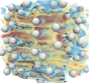
Figure 1. PR–DNS of homogeneous fluidization at  ${Re}_m=20$, $\rho _p/\rho _f=1000$ and $\langle \phi \rangle =0.1$. Arrows denote fluid streamlines; velocity magnitude shown in colour.
The evolution of granular temperature in this system is dictated by the covariance of fluctuating hydrodynamic acceleration  $\boldsymbol {a}_{h}^{\prime }$ and particle velocity $\boldsymbol {v}_{p}^{\prime }$:
 \begin{equation} \frac{{\rm d}T}{{\rm d}t} \equiv S-\varGamma =\frac{2}{3}\,\langle \boldsymbol{a}_{h}^{\prime}\boldsymbol{\cdot}\boldsymbol{v}_{p}^{\prime}\rangle, \end{equation}
which contains sources  $S$ and sinks $\varGamma$ (Tenneti, Mehrabadi & Subramaniam Reference Tenneti, Mehrabadi and Subramaniam2016). Therefore, accurate descriptions for $\boldsymbol {a}_{h}^{\prime }$ are crucial to capturing $T(t)$ in homogeneous fluidization of elastic spheres.
For a particle subjected to hydrodynamic forces, its total translational velocity  $\boldsymbol {v}_p = \langle \boldsymbol {v}_p \rangle + \boldsymbol {v}_p^{\prime }$ follows from
 \begin{equation} m_p\,\frac{{\rm d}\boldsymbol{v}_p}{{\rm d}t}=\int_{\partial \varOmega} \boldsymbol{\tau}\boldsymbol{\cdot}\boldsymbol{n}\,{\rm d}S, \end{equation}
where  $m_p$ is the particle mass, and surface integration of the fluid stress tensor $\boldsymbol {\tau }$ (comprised of pressure and viscous stress) gives the total hydrodynamic acceleration $\boldsymbol {a}_h$. A model for $\boldsymbol {a}_h(t)$ has been obtained in the limit of an isolated sphere and Stokes flow by Maxey & Riley (Reference Maxey and Riley1983); it involves a superposition of forces from the undisturbed fluid flow, quasi-steady drag, added mass and Basset history. At finite solids volume fractions and Reynolds numbers, analytical evaluation of the fluid stress integral is not tractable. Alternatively, correlations are often obtained from PR–DNS by ensemble averaging the net hydrodynamic force acting on a suspension. However, as shown in figure 1, particles interact with fluid wakes generated by their neighbours – referred to as pseudo-turbulent kinetic energy (PTKE) – leading to a distribution of hydrodynamic forces (Akiki, Jackson & Balachandar Reference Akiki, Jackson and Balachandar2016) that drive relative motion between particles. The application of a drag correlation, obtained from ensemble averaging, cannot capture the distribution in hydrodynamic force. We describe this PTKE-induced drag distribution as a stochastic process in § 3. The predictive capability of the theory is emphasized in § 4 for $\{{Re}_m \in [10, 100 ]; \langle \phi \rangle \in [0.1, 0.4 ]; \rho _p/\rho _f \in [100, 1000 ] \}$, where $\rho _p$ is the particle density, and considerations are given to low density ratio (bubbly) flows $\rho _p/\rho _f \ll 1$ in § 4.3.
3. Stochastic process and solutions
At the conditions considered here, hydrodynamic disturbances are attributed to PTKE generated by fluid boundary layers of neighbouring particles (Mehrabadi et al. Reference Mehrabadi, Tenneti, Garg and Subramaniam2015; Shallcross, Fox & Capecelatro Reference Shallcross, Fox and Capecelatro2020). Thus the drag force is decomposed into a mean contribution and a stochastic fluctuation  $\boldsymbol {a}_h^{\prime \prime }$ according to
 \begin{equation} \boldsymbol{a}_h\equiv\frac{1}{m_p}\int_{\partial \varOmega} \boldsymbol{\tau}\boldsymbol{\cdot}\boldsymbol{n}\,{\rm d}S = \frac{1}{\tau_d} \left(\langle \boldsymbol{u}_f \rangle - \boldsymbol{v}_p \right) + \boldsymbol{a}_h^{\prime\prime}, \end{equation}
where  $\tau _d =\tau _p/ F$ is the hydrodynamic time scale, $\tau _p=\rho _p d_p^2/(18 \mu _f)$ is the Stokes time scale, and $F(\langle \phi \rangle,{Re}_m)$ is a correction to Stokes drag that may be obtained from PR–DNS. Ensemble averaging (3.1) gives $\langle \boldsymbol {a}_h \rangle$. Removal of $\langle \boldsymbol {a}_h \rangle$ yields a reference frame that moves with the mean particle velocity and a fluctuating acceleration $\boldsymbol {a}_h^{\prime } = -\boldsymbol {v}_p^{\prime }/\tau _d + \boldsymbol {a}_h^{\prime \prime }$, where it is reiterated that single primes denote a fluctuation from the ensemble average, while double primes denote a stochastic fluctuation. We describe $\boldsymbol {a}_h^{\prime \prime }$ with an appropriate acceleration Langevin equation (Lattanzi et al. Reference Lattanzi, Tavanashad, Subramaniam and Capecelatro2021):
 \begin{gather} \mathrm{d}\boldsymbol{v}_p^{\prime}={-}\frac{1}{\tau_d}\,\boldsymbol{v}_p^{\prime} \, \mathrm{d}t + \boldsymbol{a}_{h}^{\prime\prime} \, \mathrm{d}t, \end{gather}
 \begin{gather}\mathrm{d}\boldsymbol{a}_{h}^{\prime\prime} ={-}\frac{1}{\tau_{a^{\prime\prime}}}\, \boldsymbol{a}_{h}^{\prime\prime} \, \mathrm{d}t + \sqrt{\frac{2}{\tau_{a^{\prime\prime}}}}\,\sigma_{a^{\prime\prime}} \,\mathrm{d}\boldsymbol{W}_t, \end{gather}
where  $\tau _{a^{\prime \prime }}$ is the integral time scale of the stochastic acceleration, $\sigma _{a^{\prime \prime }}$ is the standard deviation, and $\mathrm {d}\boldsymbol {W}_t$ is a Wiener process increment.
At this point, we consider some subtleties associated with (3.1). When applying drag correlations to PR–DNS data, Tenneti et al. (Reference Tenneti, Garg, Hrenya, Fox and Subramaniam2010) showed that incorrect dynamics for the granular temperature were obtained if the instantaneous particle velocity was utilized. In the absence of the stochastic fluctuation,  $\boldsymbol {a}_h^{\prime }$ agrees with the observations of Tenneti et al. (Reference Tenneti, Garg, Hrenya, Fox and Subramaniam2010) since velocity fluctuations can be dissipated only via $-\boldsymbol {v}_p^{\prime }/\tau _d$. However, Lattanzi et al. (Reference Lattanzi, Tavanashad, Subramaniam and Capecelatro2020) showed that $\boldsymbol {a}_h^{\prime \prime }$ leads to a covariance $\langle \boldsymbol {a}_{h}^{\prime \prime }\boldsymbol {\cdot }\boldsymbol {v}_{p}^{\prime }\rangle$ that acts as a net source to granular temperature when averaged over all of $\boldsymbol {a}_{h}^{\prime \prime }$– $\boldsymbol {v}_{p}^{\prime }$ phase space. Therefore, the fluctuating hydrodynamic acceleration $\boldsymbol {a}_h^{\prime }$ is comprised of a solely dissipative component $-\boldsymbol {v}_p^{\prime }/\tau _d$ as well as a contribution from the stochastic process $\boldsymbol {a}_h^{\prime \prime }$, which may act as a source or sink at the particle level but is overall a source when the entire suspension is considered.
Tenneti et al. (Reference Tenneti, Garg, Hrenya, Fox and Subramaniam2010) showed that sources occur when the fluctuating acceleration is aligned with the fluctuating particle velocity (quadrants 1 and 3 in  $a_h^{\prime }$– $v_p^{\prime }$ phase space), and sinks occur for the converse case (quadrants 2 and 4). To quantify $S$ and $\varGamma$, one must evaluate the quadrant-conditioned acceleration–velocity covariance; see (2.1). Thus we seek the joint probability distribution resulting from (3.2a) and (3.2b). Considering isotropic fluctuations and constant coefficients, we derive the acceleration–velocity distribution in Appendix A. Here, we report the salient result that the probability $P(v^{\prime },a^{\prime };t)=\mathcal {N}(0, \bar {\boldsymbol {\varSigma }}^{-1}(t) )$ is a normal distribution with time-dependent covariance tensor $\bar {\boldsymbol {\varSigma }}(t)$ given by
 \begin{equation} \left.\begin{gathered} \bar{\boldsymbol{\varSigma}}(t) = \left[\begin{array}{cc} \dfrac{1}{\tau_d^2}\,\sigma_{v^{\prime}}^2(t) - \dfrac{1}{\tau_d}\,\sigma_{v^{\prime}a^{\prime\prime}}(t) + \sigma_{a^{\prime\prime}}^2 & -\dfrac{1}{\tau_d}\,\sigma_{v^{\prime}}^2(t) + \sigma_{v^{\prime}a^{\prime\prime}}(t) \\ -\dfrac{1}{\tau_d}\,\sigma_{v^{\prime}}^2(t) + \sigma_{v^{\prime}a^{\prime\prime}}(t) & \sigma_{v^{\prime}}^2(t) \end{array} \right], \\ \sigma_{v^{\prime}}^2(t) = \sigma_{a^{\prime\prime}}^2 \hat{\tau}^{+} \left[ \tau_d \mathbb{E}_1 + 2 \hat{\tau}^{-} \left( \mathbb{E}_1 - \mathbb{E}_2 \right) + \mathbb{C}_0 \tau_d \left(1 - \mathbb{E}_1 \right) - 2 \rho_0\,\sqrt{\frac{\mathbb{C}_0 \tau_d}{\hat{\tau}^{+}}}\, \hat{\tau}^{-} \left( \mathbb{E}_1 - \mathbb{E}_2 \right) \right], \\ \sigma_{v^{\prime}a^{\prime\prime}}(t) = \sigma_{a^{\prime\prime}}^2 \hat{\tau}^{+} \left[ \mathbb{E}_2 + \rho_0\, \sqrt{\frac{\mathbb{C}_0 \tau_d}{\hat{\tau}^{+}}} \left( 1 - \mathbb{E}_2 \right)\right], \end{gathered}\right\} \end{equation}
where  $\mathbb {E}_1 = [ 1 - \exp ( -2t/\tau _d ) ]$, $\mathbb {E}_2 = [ 1 - \exp ( -t/\hat {\tau }^{+} ) ]$, $\hat {\tau }^{+} = \tau _d \tau _{a^{\prime \prime }} /(\tau _d + \tau _{a^{\prime \prime }})$, $\hat {\tau }^{-} = \tau _d \tau _{a^{\prime \prime }} /(\tau _d - \tau _{a^{\prime \prime }})$, $\rho _0 = \sigma _{v^{\prime }a^{\prime \prime },0}/(\sigma _{v^{\prime },0} \, \sigma _{a^{\prime \prime }})$ is the initial correlation coefficient between the fluctuating velocity and stochastic acceleration, and $\mathbb {C}_{0} \geqslant 0$ is a proportionality constant that specifies the initial velocity variance $\sigma _{v^{\prime },0}^2$ as a fraction of the steady velocity variance $\sigma _{v^{\prime },\infty }^2 = \sigma _{a^{\prime \prime }}^2 \hat {\tau }^{+} \tau _d$. Following Stuart & Ord (Reference Stuart and Ord2010), we derive relations for the quadrant-covariance of a joint-normal (see Appendix B):
 \begin{gather} S(t) = \frac{2\sqrt{\varSigma_{11} \varSigma_{22}}}{\rm \pi} \left(\rho \arcsin{\rho} + \sqrt{1-\rho^2} + \frac{\rm \pi}{2} \rho \right), \end{gather}
 \begin{gather}\varGamma(t) = \frac{2\sqrt{\varSigma_{11} \varSigma_{22}}}{\rm \pi} \left(\rho \arcsin{\rho} + \sqrt{1-\rho^2} - \frac{\rm \pi}{2} \rho \right), \end{gather}
where  $\rho (t)=\varSigma _{12}/\sqrt {\varSigma _{11} \varSigma _{22}}$ is the correlation coefficient evaluated at time $t$.
$t$.
Evaluation of (3.4) requires closure for the stochastic process. We approximate  $\tau _{a^{\prime \prime }}$ with the mean-free time between successive collisions (Chapman, Cowling & Burnett Reference Chapman, Cowling and Burnett1970):
 \begin{equation} \tau_{a^{\prime\prime}} \approx \tau_{col} = \frac{d_p}{24 \langle \phi \rangle g_0}\,\sqrt{\frac{\rm \pi}{T}}, \end{equation}
where  $g_0$ is the radial distribution function at contact (Ma & Ahmadi Reference Ma and Ahmadi1988). Details regarding motivation for $\tau _{a^{\prime \prime }} \approx \tau _{col}$ are provided in Lattanzi et al. (Reference Lattanzi, Tavanashad, Subramaniam and Capecelatro2021). Here, we summarize that the aforementioned study considers the time scale analysis of Wylie, Koch & Ladd (Reference Wylie, Koch and Ladd2003) and Mehrabadi et al. (Reference Mehrabadi, Tenneti, Garg and Subramaniam2015), which characterizes a ratio between the mean particle response time to hydrodynamic force fluctuations and the mean time between collisions. For the hydrodynamic conditions emphasized in this study, results presented in Lattanzi et al. (Reference Lattanzi, Tavanashad, Subramaniam and Capecelatro2021) suggest that the mean collisional time scale is smaller than the mean hydrodynamic time scale, i.e. the flow is collisionally dominated. Furthermore, the steady granular temperature solution derived here, and given in (4.7), leads to quantitative agreement between theory and PR–DNS data for the hydrodynamic time scale (Lattanzi et al. Reference Lattanzi, Tavanashad, Subramaniam and Capecelatro2021).
The drag time scale  $\tau _d({Re}_m,\langle \phi \rangle )$ in (3.2a) is given by Tenneti, Garg & Subramaniam (Reference Tenneti, Garg and Subramaniam2011), while the standard deviation $\sigma _{a^{\prime \prime }}$ in (3.2b) is closed with a correlation obtained from PR–DNS of freely evolving particle assemblies, given by
 \begin{gather} \sigma_{a^{\prime\prime}} = \beta\,f_{\langle \phi \rangle}^{\sigma_F}\,f_{iso}\, \frac{(1-\langle \phi \rangle)\left| \langle \boldsymbol{w} \rangle \right|}{\tau_p}, \end{gather}
 \begin{gather}f_{\langle \phi \rangle}^{\sigma_F} = 5.39\langle \phi \rangle - 4.00 \langle \phi \rangle^2 + 24.93 \langle \phi \rangle^3, \end{gather}
 \begin{gather}f_{iso} = \left( 1 + 0.15\,{Re}_m^{0.687} \right). \end{gather}
Here,  $f_{iso}$ represents the drag correction for an isolated particle using the classical correlation of Schiller & Naumann (Reference Schiller and Naumann1933). We note that the correlation provided in (3.6) differs from that of stationary particle assemblies reported in Lattanzi et al. (Reference Lattanzi, Tavanashad, Subramaniam and Capecelatro2021). Here, the $\beta$ factor is introduced to account for anisotropy. It is reiterated that stochastic fluctuations in the present theory are treated as isotropic, and the role of collisions is to redistribute components of the particle velocity fluctuations. To quantify hydrodynamic sources and sinks to granular temperature with an isotropic model, we average the force variance in all three directions. We note that $\beta$ does not drive anisotropy in the granular temperature since the model is isotropic; future work along the lines discussed in § 5 will be needed to capture such phenomena. For conditions considered here, the force variance extracted from PR–DNS is observed to be ${\sim }3$ times larger in the streamwise direction than the transverse directions (Lattanzi et al. Reference Lattanzi, Tavanashad, Subramaniam and Capecelatro2021), yielding $\beta = \sqrt {5/9}$ in the present work. We note that force anisotropy ( $\beta < 1$) may depend upon ${Re}_m$ or $\langle \phi \rangle$, and future efforts to parametrize this quantity would be beneficial.
The present correlation for drag variation is fit to PR–DNS with freely evolving particles, while the correlation provided in Lattanzi et al. (Reference Lattanzi, Tavanashad, Subramaniam and Capecelatro2021) is fit to PR–DNS with fixed particles. It has been shown that the variance in hydrodynamic force grows with  ${Re}_T = \rho _f d_p \sqrt {T}/\mu _f$ (Huang et al. Reference Huang, Wang, Zhou and Li2017). To gauge the role of particle mobility on drag variation, we consider the normalized standard deviation in streamwise hydrodynamic force for freely evolving and fixed particles (see figure 2). For $\langle \phi \rangle \geqslant 0.2$, the standard deviation in drag force is under-predicted by PR–DNS with fixed particles, when compared to freely evolving suspensions. Thus (3.6) takes the same form as that reported by Lattanzi et al. (Reference Lattanzi, Tavanashad, Subramaniam and Capecelatro2021), but with an anisotropy factor $\beta$ and a solids volume fraction correction $f_{\phi }^{\sigma _F}$ that is fit to data from PR–DNS with freely evolving particles. To this end, quantifying $\sigma _{a^{\prime \prime }}$ over a wide range of conditions would also be of great value to the present theory.

Figure 2. Standard deviation in drag force normalized by the drag force on an isolated sphere,  $F_{single} = 3 {\rm \pi}\mu _f d_p f_{iso} (1-\langle \phi \rangle )| \langle \boldsymbol {w} \rangle |$ (Schiller & Naumann Reference Schiller and Naumann1933). Symbols denote PR–DNS data with freely evolving (square) and fixed (circle) particles. The solid line denotes (3.6b), while the dashed line denotes $f_{\phi }^{\sigma _F}$ in Lattanzi et al. (Reference Lattanzi, Tavanashad, Subramaniam and Capecelatro2021); ${Re}_m= 10$ (red), ${Re}_m=20$ (blue), ${Re}_m=50$ (green), ${Re}_m=100$ (magenta). Freely evolving PR–DNS data are at $\rho _p/\rho _f = 100$.
Examining the theoretical inputs provided in (3.5)–(3.6) shows that  $\sigma _{a^{\prime \prime }}$ is constant for specified $\{ {Re}_m; \langle \phi \rangle ; \tau _p \}$, but $\tau _{a^{\prime \prime }} = f(T)$ varies in time. To account for the variable memory time scale, the constant-coefficient solutions in (3.3) are integrated forward in time by applying them to a time step $\Delta t$. More specifically, given a specified state at time $s$, the state at time $s + \Delta t$ may be obtained by formally replacing $t=\Delta t$ in (3.3). Repeating the procedure yields $\bar {\boldsymbol {\varSigma }}(t)$, which may be utilized to compute $S(t)$ and $\varGamma (t)$ (see Appendix C).
4. Results
Analytical results are first compared with PR–DNS benchmark data for two canonical flows at  ${Re}_m=20$, $\langle \phi \rangle =0.1$ and $\rho _p/\rho _f=1000$. Namely, homogeneous heating systems (HHS) and homogeneous cooling systems (HCS) are examined in detail. In the former systems, particles are given an initial granular temperature $T_0 = 0$, while the latter is initialized as $T_{0} > T_{\infty }$, with $T_{\infty }$ the steady granular temperature. Considering the dimensionless source $\hat {S}(t) = S(t)\,\tau _p/((1-\langle \phi \rangle )^2 | \langle \boldsymbol {w} \rangle |^2 )$ (This normalization is not appropriate for the case of zero mean slip where the mean hydrodynamic drag is zero but there is a purely fluctuating part; such systems could be an interesting canonical case for model development.) and analogous dimensionless sink $\hat {\varGamma }(t)$, we observe acceptable agreement between analytical predictions and PR–DNS data (see figure 3). We note that $T(t)$ is a result of integrating the difference $S(t)-\varGamma (t)$. Therefore, adding a constant to the source and sink at each time $t$ preserves the difference, rendering $T(t)$ invariant. For this reason, differences between $S(t)$ and $\varGamma (t)$ from PR–DNS and theory do not yield significant errors in the granular temperature. Physically speaking, departure between theory and simulations may be due to underlying assumptions in the model process – e.g. isotropic and constant $\sigma _{a^{\prime \prime }}$ or the Markovian Ornstein–Uhlenbeck process with exponential autocorrelation function.

Figure 3. Non-dimensional source (red) and sink (blue) in (a) HHS with  $\rho _0=1$, and (b) HCS with $\rho _0=-0.75$, at $\{ {Re}_m=20; \langle \phi \rangle =0.1; \rho _p/\rho _f=1000 \}$. (c) Evolution of non-dimensional granular temperature for HHS (red) and HCS (blue). Analytic solution obtained from (3.4) (lines), PR–DNS data (symbols); insets show the same data with linear scaling.
A direct consequence of characterizing accurately  $S(t)$ and $\varGamma (t)$ is that the theory captures the temporal evolution of ${Re}_T$ (see figure 3c). The ability of (3.3) to capture the granular temperature dynamics speaks to the statistical equivalence between the acceleration Langevin model and homogeneous fluidization of elastic particles at finite Reynolds numbers. To demonstrate equivalence at the level of joint statistics, we compare the acceleration–velocity probability distribution to scatter plots obtained from PR–DNS (see figure 4). Again, data extracted from PR–DNS are well characterized by $P(v^{\prime },a^{\prime };t)$ obtained from integration of (3.3). In HHS (figures 4a–c), granular temperature evolution is largely dominated by hydrodynamic sources (quadrants 1 and 3). By contrast, hydrodynamic sinks (quadrants 2 and 4) are dominant in HCS (figures 4d–f) since the systems are initialized with an over-prescribed velocity variance. We emphasize that both systems must satisfy a fluctuation–dissipation relation and converge to a sustained particle velocity variance that results from a balance of source and sink.

Figure 4. Joint p.d.f.s of the fluctuating particle acceleration and fluctuating particle velocity for HHS (a–c) and HCS (d–f). Analytic solution shown by colour, PR–DNS shown by symbols. The first and third quadrants correspond to sources of granular temperature, and the second and fourth quadrants correspond to dissipation.
4.1. Reynolds number and solids volume fraction effects
To examine further the scaling and robustness of solutions presented herein, we consider  ${Re}_T(t)$ at ${Re}_m \in [ 10, 100 ]$ with $\langle \phi \rangle =0.1$ and $\rho _p/\rho _f=100$ (see figure 5a). For the conditions considered, the theory predicts granular temperature evolution that is in accordance with PR–DNS results. However, we note that the ${Re}_m=100$ case shows a noticeable over-prediction for ${Re}_T$ at steady state, with relative error ${\approx }18\,\%$. It should be noted that the that the anisotropy in fluid phase kinetic energy has an anomalous dependence at $\langle \phi \rangle = 0.1$, when compared to higher solids volume fractions (Mehrabadi et al. Reference Maxey and Riley2015, Tavanashad et al. Reference Tavanashad, Passalacqua, Fox and Subramaniam2019). The anomalous anisotropy in fluid velocity fluctuations (see figures 2–3 and discussion in § 4.2 of Tavanashad et al. Reference Tavanashad, Passalacqua, Fox and Subramaniam2019) may in turn affect ${Re}_T$ through anisotropy in the force fluctuations, which are not accounted for in the current model.

Figure 5. (a) Evolution of non-dimensional granular temperature in HHS for varying Reynolds number at  $\langle \phi \rangle =0.1$, $\rho _p/\rho _f=100$, with ${Re}_m = 10$ (red), ${Re}_m = 20$ (blue), ${Re}_m = 50$ (green), ${Re}_m = 100$ (black). Evolution of non-dimensional granular temperature for varying solids volume fraction at (b) ${Re}_m =20$, $\rho _p/\rho _f=100$, and (c) $\rho _p/\rho _f=1000$, with $\langle \phi \rangle = 0.1$ (red), $\langle \phi \rangle =0.2$ (blue), $\langle \phi \rangle =0.3$ (green), $\langle \phi \rangle =0.4$ (black). Analytic solution shown by lines, PR–DNS shown by symbols.
Probing the effect of solids volume fraction, we consider  ${Re}_T(t)$ at ${Re}_m=20$ with $\langle \phi \rangle \in [ 0.1, 0.4 ]$ and $\rho _p/\rho _f =100$ (see figure 5b). Again, we observe reasonable agreement between theory and PR–DNS. Furthermore, the moderate growth in granular temperature for $\langle \phi \rangle \geqslant 0.2$ is replicated appropriately with (3.6b). Repeating the analysis for $\rho _p/\rho _f =1000$, which yields smaller steady granular temperature, again shows acceptable agreement with PR–DNS (see figure 5c). Thus the present results motivate further the notion that accurate and robust descriptions for $\sigma _{a^{\prime \prime }}$ are of significant value to the present theory.
4.2. Comparison with Stokes flow theory
In this section, we consider comparison with the theory of Koch & Sangani (Reference Koch and Sangani1999) (KS99), which was developed for inertial particles at moderate solids volume fractions and low Reynolds numbers (Stokes flow regime). The granular temperature balance for homogeneous fluidization of elastic particles (see (2.1)) is closed with KS99 theory according to
 \begin{equation} \frac{{\rm d} T}{{\rm d} t} \equiv S - \varGamma = \frac{d_p |\langle \boldsymbol{w} \rangle |^2 R_s R_{drag}^2 }{6\sqrt{{\rm \pi} } \tau_p^2 }\,T^{{-}1/2} - \frac{2 R_{diss} }{\tau_p}\,T, \end{equation}
where the coefficients appearing in (4.1) are given by
 \begin{gather} R_s = \frac{1}{g_0 \left(1 + 3.5 \langle \phi \rangle^{1/2} + 5.9 \langle \phi \rangle \right)}, \end{gather}
 \begin{gather}R_{drag} = \frac{1 + 3(\langle \phi \rangle/2)^{1/2} + (135/64) \langle \phi \rangle \ln \langle \phi \rangle + 17.14 \langle \phi \rangle}{1 + 0.681 \langle \phi \rangle - 8.48 \langle \phi \rangle^2 + 8.16 \langle \phi \rangle^3}, \end{gather}
 \begin{align} R_{diss} &= 1 + 3 (\langle \phi \rangle/2)^{1/2} + (135/64) \langle \phi \rangle \ln \langle \phi \rangle + 11.26 \langle \phi \rangle \nonumber\\ & \quad \times \left(1 - 5.1 \langle \phi \rangle + 16.57 \langle \phi \rangle^2 - 21.77 \langle \phi \rangle^3 \right) - \langle \phi \rangle g_0 \ln \varepsilon_m, \end{align}
where  $\varepsilon _m=0.01$ is the lubrication breakdown length. For homogeneous fluidization at a fixed Reynolds number, (4.1) yields a Bernoulli differential equation with constant coefficients, and may be solved analytically to obtain
 \begin{equation} T(t) = \left[ \frac{a}{b} + \left(T_0^{3/2} - \frac{a}{b} \right) \exp \left(- \frac{3 b t }{2} \right) \right]^{2/3}, \end{equation}
where  $a=d_p |\langle \boldsymbol {w} \rangle |^2 R_s R_{drag}^2 /( 6\sqrt {{\rm \pi} } \tau _p^2 )$ is the source coefficient, and $b = 2 R_{diss}/ \tau _p$ is the sink coefficient. In the long time limit, (4.5) yields a steady value
 \begin{equation} T_{\infty} = \left(|\langle \boldsymbol{w} \rangle | R_{drag}\right)^2 \left[ \frac{R_s}{6 \sqrt{\rm \pi} \,{St} \,R_{diss}}\right]^{2/3}, \end{equation}
where we emphasize that the Stokes number  ${St} = 2 \tau _p |\langle \boldsymbol {w} \rangle | R_{drag}/d_p$ is computed with the terminal velocity for an isolated sphere subject to Stokes drag, which is related to the slip velocity as $U_t = |\langle \boldsymbol {w} \rangle | R_{drag}$. Equation (4.6) reveals that $T_{\infty } \sim (\rho _p/\rho _f)^{-2/3}$ with KS99 theory.
Employing (4.5) and (4.1), the evolution of sources, sinks, and dimensionless granular temperature may be obtained readily for the conditions considered in figure 3 (see figure 6). Inspection of the source term in (4.1) shows that  $S\sim T^{-1/2}$ diverges as $T \rightarrow 0$. For the source-dominated heating system, KS99 theory predicts qualitatively incorrect evolutions for $S(t)$ when compared to PR–DNS (see figure 6a). In fact, the slopes of the lines in figure 6(a) are given by the $T$ exponent in (4.1) (namely, $-1/2, 1$) since the plot is in logarithmic scale. Since the balance in (4.1) may be formulated as an inhomogeneous first-order differential for $U = T^{3/2}$, the weakly singular source for $T$ is mapped to a constant source for $U$, thereby yielding $T(t)$ that is well-behaved in HHS. Therefore, KS99 theory predicts reasonable ${Re}_T (t)$ in HHS, but does so by treating the fluid-mediated source term as a weakly singular impulse, which is physically incorrect. These results show that the hydrodynamic acceleration vector $\boldsymbol {a}_h$, which plays a role in the Enskog equation (1.1), is not properly defined with KS99 theory. For HCS, $S$ and $\varGamma$ behaviour dramatically improves (see figure 6b); this implies that KS99 theory characterizes the hydrodynamic sink better than the source. The leading-order approximation to $\varGamma$ is expected to follow the mean drag closure (a well-characterized quantity). Since KS99 theory employs a mean drag closure for $\varGamma$, improved predictions for dissipation-dominated flows are to be expected.

Figure 6. Same as figure 3, but dashed lines correspond to the theory of Koch & Sangani (Reference Koch and Sangani1999).
Repeating the parameter sweeps in figure 5 allows us to draw direct comparisons with KS99 theory over a wide range of conditions (see figure 7). At larger Reynolds numbers  ${Re}_m > 20$, KS99 theory leads to under-predictions for the steady granular temperature, which is likely a consequence of extending the theory so far from Stokes flow (see figure 7a). At ${Re}_m = 20$, KS99 theory predicts the correct qualitative trends with increasing solids volume fraction and is in reasonable agreement with the present theory (see figures 7b,c).

Figure 7. Same as figure 5, but dashed lines correspond to the theory of Koch & Sangani (Reference Koch and Sangani1999).
4.3. Density ratio scaling
While the present theory is designed around inertial particles at high density ratios  $\rho _p / \rho _f \gg 1$, it is beneficial to consider the behaviour across density ratio. We first note that previous PR–DNS studies at $\rho _p/\rho _f \geqslant 100$ have concluded that $T_{\infty } \sim ( \rho _p/\rho _f )^{-1}$ (Tang, Peters & Kuipers Reference Tang, Peters and Kuipers2016; Tenneti et al. Reference Tenneti, Mehrabadi and Subramaniam2016), while the theory of KS99 predicts $T_{\infty } \sim (\rho _p/\rho _f)^{-2/3}$ for inertial particles subject to Stokes flow. The aforementioned scalings from PR–DNS and theory will lead to unrealistic granular temperature for low density particles $\rho _p/\rho _f \ll 1$. The PR–DNS study of Tavanashad et al. (Reference Tavanashad, Passalacqua, Fox and Subramaniam2019) showed that $T_{\infty }$ levels off at low density ratio due to the additional dissipation associated with unsteady hydrodynamic forces (e.g. added mass and Basset history). Furthermore, for ${Re}_m \in [10, 100]$ and $\langle \phi \rangle =0.1$, Tavanashad, Passalacqua & Subramaniam (Reference Tavanashad, Passalacqua and Subramaniam2021) showed that the correlation of Tenneti et al. (Reference Tenneti, Garg and Subramaniam2011) replicated the mean drag forces obtained from freely evolving PR–DNS simulations of buoyant particles down to $\rho _p/\rho _f = 0.01$. Therefore, at ${Re}_m=20, 50, 100$ and $\langle \phi \rangle =0.1$, we expect the $\tau _d$ closure employed here to be reasonably accurate across density ratio. Taking $\lim _{t\to \infty } \sigma _{v^{\prime }}^2(t)$ in (3.3), we obtain an algebraic relation for the steady granular temperature resulting from the acceleration Langevin model:
 \begin{equation} T_{\infty} = \frac{\sigma_{a^{\prime\prime}}^2 \tau_d^2\, \tau_{a^{\prime\prime}}(T_{\infty})}{\tau_d + \tau_{a^{\prime\prime}} (T_{\infty})}. \end{equation}
Solving (4.7) for  $T_{\infty }$ allows us to ascertain the behaviour of the present theory across a wide range of density ratios (see figure 8). Rather than a single power-law scaling, as deduced from inertial particle systems, the present theory predicts an exponent, $n$, that is itself a function of the density ratio, i.e. $T_{\infty } \sim ( \rho _p/\rho _f )^{n(\rho _p/\rho _f)}$. Considering the asymptotic limit of $\rho _p/\rho _f \rightarrow \infty$, one may recognize that $\tau _d \gg \tau _{a^{\prime \prime }}$, thus $T_{\infty } \sim \sigma _{a^{\prime \prime }}^2 \tau _d \tau _{a^{\prime \prime }}(T_{\infty })$. Therefore, in the limit of infinitely large density ratio, the present theory predicts $T_{\infty } \sim (\rho _p/\rho _f)^{-2/3}$, which agrees with KS99. Furthermore, it is stressed that the $n=-2/3$ scaling replicates PR–DNS data for $\rho _p/\rho _f \in [10, 1000]$ better than the correlation of Tenneti et al. (Reference Tenneti, Mehrabadi and Subramaniam2016) with $n=-1$ scaling. Examining figure 7 in Tenneti et al. (Reference Tenneti, Mehrabadi and Subramaniam2016), one may also observe the departure from $n=-1$ scaling out to $\rho _p/\rho _f = 2000$. For the asymptotic limit of $\rho _p/\rho _f \rightarrow 0$, one may recognize that $\tau _d \ll \tau _{a^{\prime \prime }}$, thus $T_{\infty } \sim \sigma _{a^{\prime \prime }}^2 \tau _d^2$. Therefore, in the limit of infinitely small density ratio, the present theory predicts $T_{\infty } \sim (\rho _p/\rho _f)^{0}$, which agrees with the PR–DNS of Tavanashad et al. (Reference Tavanashad, Passalacqua, Fox and Subramaniam2019). In summary, the theory described herein exhibits correct scaling for the granular temperature dependence upon density ratio in the asymptotically inertial and buoyant particle limits, and captures qualitatively the magnitude of the steady granular temperature across the range of density ratios considered.

Figure 8. Non-dimensional granular temperature at steady state as a function of density ratio at  ${Re}_m = 20$ (red), ${Re}_m = 50$ (blue), ${Re}_m = 100$ (black), with $\langle \phi \rangle = 0.1$ and $\rho _p/\rho _f \in [0.001, 1000]$. Analytical solutions are shown by solid lines, PR–DNS of Tavanashad et al. (Reference Tavanashad, Passalacqua, Fox and Subramaniam2019) are shown by symbols, and $n=-2/3$ scaling is shown by dotted lines.
5. Conclusion
Analytical solutions for fluid-mediated sources of granular temperature were derived from an acceleration Langevin equation, which models drag disturbances in moderately dense suspensions of elastic particles at finite Reynolds numbers. Quadrant-conditioned covariance integrals of the joint fluctuating acceleration–velocity distribution function  $P(v^{\prime },a^{\prime };t)$ yield directly the hydrodynamic source and sink. Analytical predictions for the evolution of source, sink and granular temperature are in agreement with data obtained from PR–DNS. Furthermore, the derived $P(v^{\prime },a^{\prime };t)$ agrees with acceleration–velocity scatter plots obtained from PR–DNS, and the theory predicts qualitatively correct steady granular temperature scaling for inertial and buoyant particles.
A variety of approaches may be taken when combining the present work with kinetic theory. The first, and most rigorous, approach would be to follow Garzó et al. (Reference Garzó, Tenneti, Subramaniam and Hrenya2012) and start off with the Enskog equation in (1.1). The closure for hydrodynamic acceleration then has implications on the equilibrium distribution, the solids transport coefficients and the granular temperature balance (inclusion of  $S-\varGamma$). We also emphasize that anisotropic drag forces (observed here) may then lead to an equilibrium distribution that is an anisotropic Gaussian (Vié, Doisneau & Massot Reference Vié, Doisneau and Massot2015), where anisotropy in the particle Reynolds stresses becomes a consequence of drag anisotropy and collisions. A deep dive into this first approach is of great value but beyond the scope of the present work. A second, and far simpler, approach is to append the granular temperature balance to include $S - \varGamma$. Since acceleration–velocity covariances are not transported quantities in standard two-fluid models, evaluation of $\rho _0$ in the present theory poses a challenge for inhomogeneous flows. We consider a local equilibrium approximation for this term in Appendix C.
While results presented here at low density ratio are incipient, the modelling paradigm shows promise as a viable starting place for developing a theory across particle density ratio. In this spirit, improved  $\sigma _{a^{\prime \prime }}$ correlations may be obtained and utilized alongside drag correlations that are valid across density ratio (Tavanashad et al. Reference Tavanashad, Passalacqua and Subramaniam2021). These efforts may allow extension of the present theory beyond inertial particles, i.e. a general description for fluid-mediated sources to granular temperature that is valid from gas–solid to bubbly flows appears possible.
Finally, it is noted that the present theory is built upon the assumption that hydrodynamic forces within a suspension are normally distributed. While normal distributions have been observed by the authors at many of the considered conditions  $\{{Re}_m; \langle \phi \rangle ; \rho _p/\rho _f \}$, as well as by others at similar conditions (Huang et al. Reference Huang, Wang, Zhou and Li2017; Esteghamatian et al. Reference Esteghamatian, Euzenat, Hammouti, Lance and Wachs2018; Balachandar Reference Balachandar2020), the mechanism(s) leading to normally distributed drag fluctuations pose an outstanding question. Future work that expounds upon the normal drag distribution would provide valuable insight into the regions of validity for the present theory.
Funding
This work was supported by National Science Foundation under grants CBET-1904742 and CBET-1438143.
Declaration of interests
The authors report no conflict of interest.
Appendix A. The joint acceleration–velocity distribution
A.1. Fokker–Planck solution
The system of stochastic differential equations in (3.2a) and (3.2b) may be solved in a weak (distributional) sense by considering the constant-coefficient Fokker–Planck equation in one dimension:
 \begin{equation} \frac{\partial P}{\partial t} + \frac{\partial }{\partial v^{\prime}} \left[\left(a^{\prime\prime} - \frac{1}{\tau_d}\,v^{\prime}\right)P\right] - \frac{1}{\tau_{a^{\prime\prime}}}\,\frac{\partial }{\partial a^{\prime\prime}} (a^{\prime\prime} P) = \frac{\sigma_{a^{\prime\prime}}^2}{\tau_{a^{\prime\prime}}}\, \frac{\partial^{2} P}{{\partial a^{\prime\prime}}^{2}}, \end{equation}
where  $P(v^{\prime },a^{\prime \prime };t\mid u^{\prime },b^{\prime \prime };s)$ is the transition probability density function. Applying a Fourier transform to (A1), $\mathcal {F}[ P(\boldsymbol {x};t) ] = \mathcal {P}(\boldsymbol {k};t)$, we obtain
 \begin{equation} \frac{\partial \mathcal{P}}{\partial t} + \frac{k_{v^{\prime}}}{\tau_d}\,\frac{\partial \mathcal{P}}{\partial k_{v^{\prime}}} + \left[ \frac{k_{a^{\prime\prime}}}{\tau_{a^{\prime\prime}}} - k_{v^{\prime}} \right] \frac{\partial \mathcal{P}}{\partial k_{a^{\prime\prime}}} ={-}\frac{k_{a^{\prime\prime}}^2 \sigma_{a^{\prime\prime}}^2}{ \tau_{a^{\prime\prime}}}\,\mathcal{P}. \end{equation}
Employing the method of characteristics (MOC), we seek a parametrization variable  $s$ such that
 \begin{equation} \frac{{\rm d} \mathcal{P}(t(s),k_{v^{\prime}}(s),k_{a^{\prime\prime}}(s))}{{\rm d} s} = \frac{\partial \mathcal{P}}{\partial t}\,\frac{{\rm d} t}{{\rm d} s} + \frac{\partial \mathcal{P}}{\partial k_{v^{\prime}}}\,\frac{{\rm d} k_{v^{\prime}}}{{\rm d} s} + \frac{\partial \mathcal{P}}{\partial k_{a^{\prime\prime}}}\,\frac{{\rm d} k_{a^{\prime\prime}}}{{\rm d} s}, \end{equation}
and match the coefficients of (A3) with (A2) to yield a system of equations
 \begin{gather} \frac{{\rm d} t}{{\rm d} s} = 1, \end{gather}
 \begin{gather}\frac{{\rm d} k_{v^{\prime}}}{{\rm d} s} = \frac{k_{v^{\prime}}}{\tau_d} , \end{gather}
 \begin{gather}\frac{{\rm d} k_{a^{\prime\prime}}}{{\rm d} s} = \frac{k_{a^{\prime\prime}}}{\tau_{a^{\prime\prime}}} - k_{v^{\prime}} , \end{gather}
 \begin{gather}\frac{{\rm d} \mathcal{P}}{{\rm d} s} ={-}\frac{k_{a^{\prime\prime}}^2 \sigma_{a^{\prime\prime}}^2}{ \tau_{a^{\prime\prime}}}\, \mathcal{P}. \end{gather}
Integrating the system of equations gives
 \begin{gather} t = s + C_0, \end{gather}
 \begin{gather}k_{v^{\prime}} = C_1 \exp\left(\frac{s}{\tau_d}\right), \end{gather}
 \begin{gather}k_{a^{\prime\prime}} = C_1 \hat{\tau}^{-} \exp \left( \frac{s}{\tau_d} \right) + C_2 \exp \left( \frac{s}{\tau_{a^{\prime\prime}}} \right), \end{gather}
 \begin{gather}\mathcal{P} = C_3 \exp \left(-\frac{\sigma_{a^{\prime\prime}}^2}{2 }\left[ \left(C_1 \hat{\tau}^{-}\right)^2 \frac{\tau_d}{\tau_{a^{\prime\prime}}} \exp\left(\frac{2s}{\tau_d}\right) + C_2^2 \exp \left( \frac{2s}{\tau_{a^{\prime\prime}}} \right)\right.\right.\nonumber\\ + \left.\left. 4 C_1 C_2\, \frac{\hat{\tau}^{-} \hat{\tau}^{+}}{\tau_{a^{\prime\prime}}} \exp \left( \frac{s}{\hat{\tau}^{+}} \right) \right]\vphantom{\left(-\frac{\sigma_{a^{\prime\prime}}^2}{2 }\left[ \left(C_1 \hat{\tau}^{-}\right)^2 \frac{\tau_d}{\tau_{a^{\prime\prime}}} \exp\left(\frac{2s}{\tau_d}\right) + C_2^2 \exp \left( \frac{2s}{\tau_{a^{\prime\prime}}} \right)\right.\right.}\right), \end{gather}
where  $\hat {\tau }^{-} = \tau _d \tau _{a^{\prime \prime }} /(\tau _d - \tau _{a^{\prime \prime }})$ and $\hat {\tau }^{+} = \tau _d \tau _{a^{\prime \prime }} /(\tau _d + \tau _{a^{\prime \prime }})$. Taking $C_0 = 0$, we show that the MOC solution is invertible:
 \begin{gather} s = t , \end{gather}
 \begin{gather}C_1 = k_{v^{\prime}} \exp\left(-\frac{t}{\tau_d}\right), \end{gather}
 \begin{gather}C_2 = \left[ k_{a^{\prime\prime}} - k_{v^{\prime}} \hat{\tau}^{-} \right] \exp \left( -\frac{t}{\tau_{a^{\prime\prime}}} \right). \end{gather}
A.2. Arbitrarily correlated initial condition
We consider particles with specified initial velocity variance  $\sigma _{v^{\prime },0}^2$ and initial acceleration–velocity covariance $\sigma _{v^{\prime }a^{\prime \prime },0} = \rho _0 \sigma _{a^{\prime \prime }} \sigma _{v^{\prime },0}$. The initial condition allows us to consider general fluidization, which will encompass the cooling and heating systems probed by PR–DNS studies (Tenneti et al. Reference Tenneti, Garg, Hrenya, Fox and Subramaniam2010, Reference Tenneti, Mehrabadi and Subramaniam2016; Tavanashad et al. Reference Tavanashad, Passalacqua, Fox and Subramaniam2019). The correlated initial condition yields
 \begin{equation} \mathcal{F} \left[ \mathcal{N}( \bar{\boldsymbol{\varSigma}}^{{-}1} ) \right] = \exp\left(-\frac{ k_{a^{\prime\prime}}^2 \sigma_{a^{\prime\prime}}^2}{2} -\frac{ k_{v^{\prime}}^2 \sigma_{v^{\prime},0}^2 }{2} - k_{a^{\prime\prime}} k_{v^{\prime}} \sigma_{v^{\prime}a^{\prime\prime},0} \right), \end{equation}
where  $\mathcal {N}( \bar {\boldsymbol {\varSigma }}^{-1} )$ is the normal distribution with covariance matrix $\bar {\boldsymbol {\varSigma }}$. Evaluating (A7) at $k_i(0)$ gives the initial condition
 \begin{equation} \mathcal{P}(0) = \exp\left(-\frac{\sigma_{a^{\prime\prime}}^2}{2}\left[ \left(C_1 \hat{\tau}^{-}\right)^2 \!+\! C_2^2 \!+\! 2 C_1 C_2 \hat{\tau}^{-} \right] - \frac{\sigma_{v^{\prime},0}^2}{2}\,C_1^2 - \sigma_{v^{\prime}a^{\prime\prime},0} \left[C_1^2 \hat{\tau}^{-} + C_1 C_2 \right] \right), \end{equation}
which allows the  $C_3$ constant in (A5d) to be obtained:
 \begin{align} C_3 &= \exp \left( \frac{\sigma_{a^{\prime\prime}}^2}{2}\left[ \left(C_1 \hat{\tau}^{-}\right)^2 \left(\frac{\tau_d}{\tau_{a^{\prime\prime}}} - 1\right) + 4C_1 C_2\,\frac{\hat{\tau}^{-} \hat{\tau}^{+}}{\tau_{a^{\prime\prime}}} - 2C_1C_2\hat{\tau}^{-} \right] \right) \nonumber\\ &\quad \times \exp \left( - \frac{\sigma_{v^{\prime},0}^2}{2}\,C_1^2 - \sigma_{v^{\prime}a^{\prime\prime},0} \left[C_1^2 \hat{\tau}^{-} + C_1 C_2 \right] \right). \end{align}
After inverting the constants ( $C_1$; $C_2$), and a considerable amount of algebra, the joint distribution solution in wave space is obtained:
 \begin{gather} \mathcal{P} (k_{v^{\prime}},k_{a^{\prime\prime}};t) = \exp \left( -\frac{k_{a^{\prime\prime}}^2}{2}\,\sigma_{a^{\prime\prime}}^2 - \frac{k_{v^{\prime}}^2}{2}\, \sigma_{v^{\prime}}^2(t) - k_{a^{\prime\prime}} k_{v^{\prime}} \sigma_{v^{\prime}a^{\prime\prime}}(t) \right), \end{gather}
 \begin{gather}\sigma_{v^{\prime}}^2(t) = \sigma_{a^{\prime\prime}}^2 \hat{\tau}^{+} \left[ \tau_d \mathbb{E}_2 + 2 \hat{\tau}^{-} \left( \mathbb{E}_2 - \mathbb{E}_3 \right) + \mathbb{C}_0 \tau_d \left(1 - \mathbb{E}_2 \right) - 2 \rho_0 \sqrt{\frac{\mathbb{C}_0 \tau_d}{\hat{\tau}^{+}}}\,\hat{\tau}^{-} \left( \mathbb{E}_2 - \mathbb{E}_3 \right) \right], \end{gather}
 \begin{gather}\sigma_{v^{\prime}a^{\prime\prime}}(t) = \sigma_{a^{\prime\prime}}^2 \hat{\tau}^{+} \left[ \mathbb{E}_3 + \rho_0 \sqrt{\frac{\mathbb{C}_0 \tau_d}{\hat{\tau}^{+}}} \left( 1 - \mathbb{E}_3 \right)\right], \end{gather}
 \begin{gather}\mathbb{E}_2 = \left\{ 1 - \exp \left( -\frac{2t}{\tau_d} \right) \right\}, \end{gather}
 \begin{gather}\mathbb{E}_3 = \left\{ 1 - \exp \left( -\frac{t}{\hat{\tau}^{+}} \right) \right\}. \end{gather}
Here,  $\mathbb {C}_{0} \geqslant 0$ is a proportionality constant that specifies the initial velocity variance $\sigma _{v^{\prime },0}^2$ as a fraction of the steady velocity variance $\sigma _{v^{\prime },\infty }^2 = \sigma _{a^{\prime \prime }}^2 \hat {\tau }^{+} \tau _d$. Similarly, $\rho _0 \in [-1, 1 ]$ is the initial correlation coefficient that specifies the initial covariance $\sigma _{v^{\prime }a^{\prime \prime },0}$. Since (A10a) is joint-normal in wave space, it will also be joint-normal in physical space. Furthermore, taking $\lim \mathbb {C}_0 \rightarrow 0$ and $\lim \rho _0 \rightarrow 0$ shows that the velocity variance $\sigma _{v^{\prime }}^2(t)$ and acceleration–velocity covariance $\sigma _{v^{\prime }a^{\prime \prime }}(t)$ match the solutions provided in Lattanzi et al. (Reference Lattanzi, Tavanashad, Subramaniam and Capecelatro2020).
A.3. Total acceleration distribution
The total fluctuating hydrodynamic acceleration  $\boldsymbol {a}_{h}^{\prime }$ (see right-hand side of (3.2a)) includes contributions from deterministic drag and stochastic fluctuations:
 \begin{equation} \boldsymbol{a}_{h}^{\prime} ={-}\frac{1}{\tau_d}\, \boldsymbol{v}_{p}^{\prime} + \boldsymbol{a}_{h}^{\prime\prime}. \end{equation}
To compare with PR–DNS, we require  $P(\boldsymbol {v}^{\prime },\boldsymbol {a}^{\prime };t)$ rather than $P(\boldsymbol {v}^{\prime },\boldsymbol {a}^{\prime \prime };t)$. Thus we seek to characterize the variances and covariances of total fluctuating hydrodynamic acceleration. The covariance tensors are given by
 \begin{gather} \left\langle \boldsymbol{a}_{h}^{\prime} \otimes \boldsymbol{a}_{h}^{\prime} \right\rangle = \frac{1}{\tau_d^2} \left\langle \boldsymbol{v}_{p}^{\prime} \otimes \boldsymbol{v}_{p}^{\prime} \right\rangle - \frac{1}{\tau_d} \left\langle \boldsymbol{v}_{p}^{\prime} \otimes \boldsymbol{a}_{h}^{\prime\prime} \right\rangle + \left\langle \boldsymbol{a}_{h}^{\prime\prime} \otimes \boldsymbol{a}_{h}^{\prime\prime} \right\rangle, \end{gather}
 \begin{gather}\left\langle \boldsymbol{v}_{p}^{\prime} \otimes \boldsymbol{a}_{h}^{\prime} \right\rangle ={-}\frac{1}{\tau_d} \left\langle \boldsymbol{v}_{p}^{\prime} \otimes \boldsymbol{v}_{p}^{\prime} \right\rangle + \left\langle \boldsymbol{v}_{p}^{\prime} \otimes \boldsymbol{a}_{h}^{\prime\prime} \right\rangle. \end{gather}
Substituting results from (A10b) and (A10c), we then obtain
 \begin{gather} \sigma_{a^{\prime}}^2 = \frac{1}{\tau_d^2}\,\sigma_{v^{\prime}}^2 - \frac{1}{\tau_d}\sigma_{v^{\prime}a^{\prime\prime}} + \sigma_{a^{\prime\prime}}^2, \end{gather}
 \begin{gather}\sigma_{v^{\prime} a^{\prime}} ={-}\frac{1}{\tau_d}\,\sigma_{v^{\prime}}^2 + \sigma_{v^{\prime}a^{\prime\prime}} . \end{gather}
Therefore, the fluctuating acceleration–velocity distribution  $P(\boldsymbol {v}^{\prime },\boldsymbol {a}^{\prime };t)$ is a normal distribution $\mathcal {N}(\bar {\boldsymbol {\varSigma }}^{-1} )$ with time-dependent covariance tensor given by
 \begin{equation} \bar{\boldsymbol{\varSigma}} = \left[ \begin{array}{cc} \sigma_{a^{\prime}}^2(t) & \sigma_{v^{\prime} a^{\prime}}(t)\\[3pt] \sigma_{v^{\prime} a^{\prime}}(t) & \sigma_{v^{\prime}}^2(t) \end{array} \right]. \end{equation}
Appendix B. Evaluation of quadrant-covariance integrals
To quantify the sources and sinks produced by the acceleration Langevin model, the quadrant-conditioned covariances must be computed:
 \begin{align} 2 \langle v^{\prime}a^{\prime} \rangle \equiv S - \varGamma &= 4\int_{0}^{\infty} \int_{0}^{\infty} v^{\prime}a^{\prime} \, \mathcal{N}(\bar{\boldsymbol{\varSigma}}^{{-}1})\, {\rm d}a^{\prime} \, {\rm d} v^{\prime} \nonumber\\ &\quad - 4\int_{-\infty}^{0} \int_{0}^{\infty} v^{\prime}a^{\prime} \, \mathcal{N}(\bar{\boldsymbol{\varSigma}}^{{-}1})\, {\rm d}a^{\prime} \, {\rm d} v^{\prime}, \end{align}
where  $\mathcal {N}(\bar {\boldsymbol {\varSigma }}^{-1})$ is the derived normal probability distribution with covariance matrix given in (A14). To evaluate the integrals given in (B1), we proceed similarly to the derivation provided in Stuart & Ord (Reference Stuart and Ord2010). For the source integral, substituting the Fourier transform of the characteristic function in place of the normal distribution function yields
 \begin{equation} S = \frac{4}{(2{\rm \pi})^2} \int_{0}^{\infty} \int_{0}^{\infty} x_1 x_2 \int_{-\infty}^{\infty} \int_{-\infty}^{\infty} \exp\left(-{\rm i}\boldsymbol{k}^{\rm T}\boldsymbol{x} - \frac{1}{2}\,\boldsymbol{k}^{\rm T} \bar{\boldsymbol{\varSigma}} \boldsymbol{k}\right) {\rm d}\boldsymbol{k} \, {\rm d}\kern0.06em \boldsymbol{x}, \end{equation}
where  $\boldsymbol {x} = [v^{\prime } \ a^{\prime } ]^\textrm {T}$ and $\boldsymbol {k} = [k_{v^{\prime }} \ k_{a^{\prime }}]^\textrm {T}$. Exchanging the order of integration and employing the identity
 \begin{equation} x_{j} \exp ( -{\rm i} k_j x_j ) = {\rm i}\,\frac{\partial }{\partial k_j} \left(\exp ( -{\rm i} k_j x_j ) \right), \end{equation}
where no summation over  $j$ is implied, leads to
 \begin{equation} S = \frac{1}{{\rm \pi}^2} \int_{-\infty}^{\infty} \int_{-\infty}^{\infty} \exp\left(-\frac{1}{2}\,\boldsymbol{k}^{\rm T} \bar{\boldsymbol{\varSigma}} \boldsymbol{k}\right) \prod_{j=1}^{2}\left( {\rm i}\, \frac{\partial }{\partial k_j} \right) \int_{0}^{\infty} \int_{0}^{\infty} \exp(-{\rm i}\boldsymbol{k}^{\rm T}\boldsymbol{x})\, {\rm d}\kern0.06em \boldsymbol{x} \, {\rm d}\boldsymbol{k}. \end{equation}
The innermost integrals over  $\boldsymbol {x}$ may be interpreted as the Fourier transforms of the Heaviside function, which have principal values $\prod _j (\textrm {i} k_j )^{-1}$. After evaluating the derivatives, one obtains
 \begin{equation} S = \frac{1}{{\rm \pi}^2} \int_{-\infty}^{\infty} \int_{-\infty}^{\infty} \exp\left(-\frac{1}{2}\,\boldsymbol{k}^{\rm T} \bar{\boldsymbol{\varSigma}} \boldsymbol{k}\right) \frac{1}{k_{v^{\prime}}^2 k_{a^{\prime}}^2}\, {\rm d}\boldsymbol{k}. \end{equation}
The exponential in (B5) will contain a covariance term  $-\rho \sigma _{v^{\prime }} \sigma _{a^{\prime }} k_{v^{\prime }} k_{a^{\prime }}$, where $\rho$ is the correlation coefficient. Differentiating both sides twice with respect to $\rho$ yields
 \begin{equation} \frac{{\rm d}^2S}{{\rm d}\rho^2} = \frac{\sigma_{v^{\prime}}^2 \sigma_{a^{\prime}}^2}{{\rm \pi}^2} \int_{-\infty}^{\infty} \int_{-\infty}^{\infty} \exp\left(-\frac{1}{2}\,\boldsymbol{k}^{\rm T} \bar{\boldsymbol{\varSigma}} \boldsymbol{k}\right) {\rm d}\boldsymbol{k}. \end{equation}
The above integral will yield the reciprocal of the normalization constant for a bi-normal distribution:
 \begin{equation} \frac{{\rm d}^2S}{{\rm d}\rho^2} \equiv \frac{\sigma_{v^{\prime}}^2 \sigma_{a^{\prime}}^2}{{\rm \pi}^2}\,2 {\rm \pi}\left| \bar{\boldsymbol{\varSigma}} \right|^{{-}1/2} = \frac{2\sigma_{v^{\prime}} \sigma_{a^{\prime}}}{\rm \pi}\, \frac{1}{\sqrt{1 - \rho^2}}. \end{equation}
Integrating twice and determining the constants – e.g. for sources  $S=0$, $\rho = -1$ and $S=2\sigma _{v^{\prime }} \sigma _{a^{\prime }}$, $\rho = 1$ – yields
 \begin{gather} S = \frac{2\sigma_{v^{\prime}} \sigma_{a^{\prime}}}{\rm \pi} \left(\rho \arcsin{\rho} + \sqrt{1-\rho^2} + \frac{\rm \pi}{2} \rho \right), \end{gather}
 \begin{gather}\varGamma = \frac{2\sigma_{v^{\prime}} \sigma_{a^{\prime}}}{\rm \pi} \left(\rho \arcsin{\rho} + \sqrt{1-\rho^2} - \frac{\rm \pi}{2} \rho \right). \end{gather}
Appendix C. Model implementation
C.1. Integration of the constant-coefficient solution
To compute  $T(t)$, $S(t)$ and $\varGamma (t)$ from the constant-coefficient solution in (3.3) and covariance integrals in (3.4), we consider an implicit Euler discretization of the granular temperature balance
 \begin{equation} T^{n+1} = T^{n} + \Delta t ( S^{n+1} - \varGamma^{n+1} ), \end{equation}
where  $n$ is the previous time step. When evaluating $S^{n+1}$ and $\varGamma ^{n+1}$, we hold the coefficients in (3.3) fixed and apply the solution to a time step $\Delta t$ (consistent with the non-anticipating nature of Itô integrals):
 \begin{equation} {\bar{\boldsymbol{\varSigma}}}^{n+1} = \left[ \begin{array}{cc} \dfrac{1}{\tau_d^2}\,\sigma_{v^{\prime}}^2(\Delta t) - \dfrac{1}{\tau_d}\,\sigma_{v^{\prime}a^{\prime\prime}}(\Delta t) + \sigma_{a^{\prime\prime}}^2 & -\dfrac{1}{\tau_d}\,\sigma_{v^{\prime}}^2(\Delta t) + \sigma_{v^{\prime}a^{\prime\prime}}(\Delta t)\\ -\dfrac{1}{\tau_d}\,\sigma_{v^{\prime}}^2(\Delta t) + \sigma_{v^{\prime}a^{\prime\prime}}(\Delta t) & \sigma_{v^{\prime}}^2(\Delta t) \end{array} \right]. \end{equation}
For completeness, we consider the computation of  $\sigma _{v^{\prime }a^{\prime \prime }}(\Delta t)$ as an example and note that the other terms in (C2) will follow the same form:
 \begin{equation} \sigma_{v^{\prime}a^{\prime\prime}}^{n+1} = {\sigma_{a^{\prime\prime}}^{2}} {\hat{\tau}^{+ \, n}} \left[ \Delta \mathbb{E}_2 + \rho_0^{n}\,\sqrt{\frac{\mathbb{C}_0^{n} \tau_d}{\hat{\tau}^{+ \, n}}} \left( 1 - \Delta \mathbb{E}_2 \right)\right], \end{equation}
where  $\Delta \mathbb {E}_1 = [ 1 - \exp ( -2\Delta t/\tau _d ) ]$, $\Delta \mathbb {E}_2 = [ 1 - \exp ( -\Delta t/\hat {\tau }^{+} ) ]$, and all coefficients on the right-hand side are evaluated at the previous time step $n$. As noted in the main text, $\sigma _{a^{\prime \prime }}^{2}$ and $\tau _d$ are constants in homogeneous fluidization that depend only upon $\{ {Re}_m; \langle \phi \rangle ; \tau _p \}$. Therefore, $\tau _{a^{\prime \prime }}$, $\mathbb {C}_0$ and $\rho _0$ are the base quantities that must be updated at each time step. Evaluation of these terms at the previous time step $n$ may be completed as follows:
 \begin{gather} \tau_{a^{\prime\prime}}^{n} = \frac{d_p}{24 \langle \phi \rangle g_0} \sqrt{\frac{\rm \pi}{T^{n}}}, \end{gather}
 \begin{gather}\mathbb{C}_0^{n} = \frac{T^{n}}{\sigma_{a^{\prime\prime}}^2 \tau_d {\hat{\tau}^{+ \, n}} }, \end{gather}
 \begin{gather}\rho_0^{n} = \frac{\sigma_{v^{\prime}a^{\prime\prime}}^{n}}{\sqrt{\sigma_{a^{\prime\prime}}^{2} T^{n} }}, \end{gather}
where we note that  $T \rightarrow 0$ leads to $\tau _{a^{\prime \prime }} \rightarrow \infty$ and $\hat {\tau }^{\pm } \rightarrow \pm \tau _d$. That is, the mean-free time diverges as the granular temperature tends to zero, but all coefficients in the solution remain bounded. Given initial conditions $T_0 = \sigma _{v^{\prime },0}^2$ and $\rho _0 = \sigma _{v^{\prime }a^{\prime \prime },0}/\left (\sqrt {T_0 \, \sigma _{a^{\prime \prime }}^2 }\right )$, the coefficients at the previous time step $n$ may be computed readily and utilized to obtain the covariance matrix at the current time step, ${\bar {\boldsymbol {\varSigma }}}^{n+1}$. The source and sink terms then become
 \begin{gather} S^{n+1} = \frac{2\sqrt{\varSigma_{11}^{n+1} \varSigma_{22}^{n+1} }}{\rm \pi} \left(\rho^{n+1} \arcsin{\rho^{n+1} } + \sqrt{1-\left(\rho^{n+1}\right)^2} + \frac{\rm \pi}{2} \rho^{n+1} \right), \end{gather}
 \begin{gather}\varGamma^{n+1} = \frac{2\sqrt{\varSigma_{11}^{n+1} \varSigma_{22}^{n+1} }}{\rm \pi} \left(\rho^{n+1} \arcsin{\rho^{n+1} } + \sqrt{1-\left(\rho^{n+1}\right)^2} - \frac{\rm \pi}{2} \rho^{n+1} \right), \end{gather}
where  $\rho ^{n+1} = \varSigma _{12}^{n+1}/\sqrt {\varSigma _{11}^{n+1} \varSigma _{22}^{n+1} }$. Repeating the process yields the reported evolution curves.
C.2. Approximations for inelastic particles and inhomogeneous flows
While the present study does not aim to tackle the general problem of inhomogeneous flows with inelastic particles, some ad hoc extensions of the current theory may be deduced readily. For homogeneous fluidization, explicitly including the collisional dissipation from KS99 into (C1) leads to
 \begin{equation} T^{n+1} = T^{n} + \Delta t \left( S^{n+1} - \varGamma^{n+1} - \frac{16 (1-e) \langle \phi \rangle g_0}{d_p \sqrt{\rm \pi}}\,({T^{n}})^{3/2} \right) , \end{equation}
where  $e \in [0, 1]$ is the restitution coefficient. It is now emphasized that the continuous form of (C8) does not match the moment equation for granular temperature resulting from (A1), since collisional dissipation was omitted from that derivation. For this reason, there exists an aliasing error where $T^{n+1} \neq ({\sigma _{v^{\prime }}^2})^{n+1}$. This is not the case for elastic particles in § C.1 where the moment equations match and thus $T^{n+1} = ({\sigma _{v^{\prime }}^2})^{n+1}$. By utilizing the granular temperature from the previous time step $T^{n}$ when computing coefficients (e.g. (C4)), rather than the value predicted without collisional dissipation $({\sigma _{v^{\prime }}^2})^{n}$, we account approximately for the aliasing error. Considering $e=0.5$, we obtain results in HHS and HCS that are comparable to the numerical integration of KS99 theory (see figure 9). We note that the PR–DNS data in figure 9 correspond to $e=1$ and thus should not match either of the lines. The PR-DNS data are included for reference to show the decrease in steady granular temperature and time required to reach steady state.

Figure 9. Same conditions as figure 3, with  $e=0.5$ in the present theory (solid lines) and KS99 (dashed lines). PR–DNS markers employ $e=1$ and are shown just for reference.
For inhomogeneous flows, specifying  $\rho _0$ poses a challenge since acceleration–velocity covariances are not transported quantities in classical kinetic theory. We emphasize that $\sigma _{v^{\prime }a^{\prime \prime }}(t)$ derived here is a consequence of solving a balance relation for this moment – i.e. the ordinary differential obtained by multiplying (A1) by $a^{\prime \prime } v^{\prime }$ and integrating over $a^{\prime \prime }$ and $v^{\prime }$ space. For homogeneous systems, only an initial condition is required to solve the ordinary differential equation. By contrast, inhomogeneous flows would require the general balance relation obtained by taking the acceleration–velocity moment of (1.1). Since granular kinetic theories neglect $\boldsymbol {a}_h$ in (1.1), transport equations for this cross-moment are generally ignored. Therefore, within an Euler–Euler framework, $T^{n}$ would be known at each computational cell (result of solution to granular temperature balance), but $\sigma _{v^{\prime }a^{\prime \prime }}^{n}$ would not be known. The simplest extension of the present theory to inhomogeneous flows requires a local equilibrium approximation in each computational cell:
 \begin{gather} \sigma_{v^{\prime}a^{\prime\prime}}^{n} \approx \sigma_{v^{\prime}a^{\prime\prime}, \infty} = {\sigma_{a^{\prime\prime}}^{2}} {\hat{\tau}^{+ \, n}}, \end{gather}
 \begin{gather}\rho_0^{n} = \min \left( \frac{ \sigma_{a^{\prime \prime}} \hat{\tau}^{+ \, n} }{\sqrt{ T^{n} }}, 1 \right). \end{gather}
Acceptable results are obtained with the local equilibrium approximation in HHS and HCS (see figure 10).


 Open access