


1 Introduction
Elucidation of the mechanisms of turbulent thermal convection in very-low-Prandtl-number fluids is crucial for our understanding of the universe and the advancement of cooling technology. Turbulent thermal convection takes place, for example, on the surfaces of stars, where the Prandtl number ( $Pr$) varies from $10^{-8}$ to $10^{-4}$ (Spiegel Reference Spiegel1962; Hanasoge, Gizon & Sreenivasan Reference Hanasoge, Gizon and Sreenivasan2016). Furthermore, turbulent thermal convection in liquid metals ( $Pr\ll 1$) is relevant in engineering applications, especially in cooling systems of tokamaks and fast breeder reactors (Zhilin et al. Reference Zhilin, Sviridov, Razuvanov, Ivochkin, Listratov, Sviridov and Belyaev2009; Belyaev et al. Reference Belyaev, Genin, Listratov, Melnikov, Sviridov, Sviridov, Ivochkin, Razuvanov and Shpansky2013). Liquid sodium is of particular interest because of its very low Prandtl number ( $Pr\approx 0.009$) and it is widely used as cooling agent in fast neutron reactors (Heinzel et al. Reference Heinzel, Hering, Konys, Marocco, Litfin, Mueller, Pacio, Schroer, Stieglitz and Stoppel2017).
One classical model of thermal convection is Rayleigh–Bénard convection (RBC), where the fluid is confined between a heated lower plate and a cooled upper plate, and the main driving force is buoyancy. The temperature inhomogeneity varies the fluid density, which in presence of gravity leads to the convective fluid motion. For reviews on RBC we refer to Bodenschatz, Pesch & Ahlers (Reference Bodenschatz, Pesch and Ahlers2000), Ahlers, Grossmann & Lohse (Reference Ahlers, Grossmann and Lohse2009), Lohse & Xia (Reference Lohse and Xia2010) and Chillà & Schumacher (Reference Chillà and Schumacher2012).
Thermal convection inevitably arises in the case of a horizontal temperature gradient. This is known as vertical convection (VC), convection in cavities or side-heated convection. In vertical convection, the heated and cooled plates are located parallel to the gravity vector and shear plays the key role, see Ng et al. (Reference Ng, Ooi, Lohse and Chung2015, Reference Ng, Ooi, Lohse and Chung2017) and Shishkina (Reference Shishkina2016).
The concept of inclined convection (IC) is a generalisation of RBC and VC, i.e. the fluid layer between the parallel plates is tilted with respect to the direction of gravity, and both buoyancy and shear act on the flow. This type of convection was studied previously by Daniels, Wiener & Bodenschatz (Reference Daniels, Wiener and Bodenschatz2003), Chillà et al. (Reference Chillà, Rastello, Chaumat and Castaing2004), Sun, Xi & Xia (Reference Sun, Xi and Xia2005), Ahlers, Brown & Nikolaenko (Reference Ahlers, Brown and Nikolaenko2006b), Riedinger et al. (Reference Riedinger, Tisserand, Seychelles, Castaing and Chillá2013), Weiss & Ahlers (Reference Weiss and Ahlers2013) and Langebach & Haberstroh (Reference Langebach, Haberstroh and Weisend2014), and more recently by Frick et al. (Reference Frick, Khalilov, Kolesnichenko, Mamykin, Pakholkov, Pavlinov and Rogozhkin2015), Mamykin et al. (Reference Mamykin, Frick, Khalilov, Kolesnichenko, Pakholkov, Rogozhkin and Vasiliev2015), Vasil’ev et al. (Reference Vasil’ev, Kolesnichenko, Mamykin, Frick, Khalilov, Rogozhkin and Pakholkov2015), Kolesnichenko et al. (Reference Kolesnichenko, Mamykin, Pavlinov, Pakholkov, Rogozhkin, Frick, Khalilov and Shepelev2015), Shishkina & Horn (Reference Shishkina and Horn2016), Teimurazov & Frick (Reference Teimurazov and Frick2017), Mandrykin & Teimurazov (Reference Mandrykin and Teimurazov2019), Khalilov et al. (Reference Khalilov, Kolesnichenko, Pavlinov, Mamykin, Shestakov and Frick2018) and Zwirner & Shishkina (Reference Zwirner and Shishkina2018).
In thermal convection, the global flow structures and heat and momentum transport are determined mainly by the following system parameters: the Rayleigh number  $Ra$, the Prandtl number $Pr$ and the aspect ratio of the container $\unicode[STIX]{x1D6E4}$. These are defined as
 $$\begin{eqnarray}Ra\equiv \unicode[STIX]{x1D6FC}g\unicode[STIX]{x0394}L^{3}/(\unicode[STIX]{x1D705}\unicode[STIX]{x1D708}),\quad Pr\equiv \unicode[STIX]{x1D708}/\unicode[STIX]{x1D705},\quad \unicode[STIX]{x1D6E4}\equiv D/L,\end{eqnarray}$$
 respectively. Here,  $\unicode[STIX]{x1D6FC}$ denotes the isobaric thermal expansion coefficient, $\unicode[STIX]{x1D708}$ the kinematic viscosity, $\unicode[STIX]{x1D705}$ the thermal diffusivity of the fluid, $g$ the acceleration due to gravity, $\unicode[STIX]{x1D6E5}\equiv T_{+}-T_{-}$ the difference between the temperatures at the heated plate ( $T_{+}$) and at the cooled plate ( $T_{-}$), $L$ the distance between the plates and $D$ the diameter of the plates.
The main response characteristics of a natural convective system are the mean total heat flux across the heated/cooled plates,  $q$, normalised by the conductive part of the total heat flux, $\hat{q}$, i.e. the Nusselt number $Nu$, and the Reynolds number $Re$:
$Re$:
 $$\begin{eqnarray}\displaystyle Nu\equiv q/\hat{q},\quad Re\equiv LU/\unicode[STIX]{x1D708}. & & \displaystyle\end{eqnarray}$$
 Here,  $U$ is the reference velocity, which is usually determined by either the maximum of the time-averaged velocity along the plates or by $\langle \boldsymbol{u}\boldsymbol{\cdot }\boldsymbol{u}\rangle ^{1/2}$, i.e. it is based on the mean kinetic energy; $\boldsymbol{u}$ is the velocity vector field and $\langle \cdot \rangle$ denotes the average in time and over the whole convection cell. Note that, even for a fixed set-up in natural thermal convection with no additional shear imposed on the system, the scaling relations of the mean heat and momentum transport, represented by $Nu$ and $Re$, with the input parameters $Ra$ and $Pr$, are not universal and are influenced by non-Oberbeck–Boussinesq (NOB) effects, see Kraichnan (Reference Kraichnan1962), Grossmann & Lohse (Reference Grossmann and Lohse2000), Ahlers et al. (Reference Ahlers, Brown, Araujo, Funfschilling, Grossmann and Lohse2006a, Reference Ahlers, Grossmann and Lohse2009), Lohse & Xia (Reference Lohse and Xia2010), Shishkina, Grossmann & Lohse (Reference Shishkina, Grossmann and Lohse2016a), Shishkina, Weiss & Bodenschatz (Reference Shishkina, Weiss and Bodenschatz2016b) and Weiss et al. (Reference Weiss, He, Ahlers, Bodenschatz and Shishkina2018).
Here, one should note that, apart from  $Pr$ and $Ra$, the geometrical confinement of the convection cell also determines the strength of the heat transport (Huang et al. Reference Huang, Kaczorowski, Ni and Xia2013; Chong et al. Reference Chong, Huang, Kaczorowski and Xia2015; Chong & Xia Reference Chong and Xia2016). Thus, in experiments by Huang et al. (Reference Huang, Kaczorowski, Ni and Xia2013) for $Pr=4.38$, an increase of $Nu$ due to the cell confinement was obtained, while in the direct numerical simulations (DNS) by Wagner & Shishkina (Reference Wagner and Shishkina2013) for $Pr=0.786$, the heat and mass transport gradually reduced with increasing confinement. This virtual contradiction was recently resolved in Chong et al. (Reference Chong, Wagner, Kaczorowski, Shishkina and Xia2018). It was found that $Pr$ determines whether the optimal $\unicode[STIX]{x1D6E4}$, at which the maximal heat transport takes place, exists or not. For $Pr>0.5$ ( $Ra=10^{8}$) an enhancement of $Nu$ was observed, where the optimal $\unicode[STIX]{x1D6E4}$ decreases with increasing $Pr$, but for $Pr\leqslant 0.5$ a gradual reduction of the heat transport with increasing confinement was obtained. For all $Pr$, the confinement induced friction causes a reduction of $Re$.
$Re$.
In the general case of inclined thermal convection, the cell inclination angle  $\unicode[STIX]{x1D6FD}$ ( $\unicode[STIX]{x1D6FD}=0^{\circ }$ in RBC and $\unicode[STIX]{x1D6FD}=90^{\circ }$ in VC) is an influential input parameter of the convective system, apart from $Ra$,
$Ra$,  $Pr$ and the geometry of the container. Experimental studies of inclined thermal liquid-sodium convection in cylinders of different aspect ratios, showed that the convective heat transfer between the heated and cooled surfaces of the container is most efficient neither in a standing position of the cylinder ( $\unicode[STIX]{x1D6FD}=0^{\circ }$), nor in a lying position ( $\unicode[STIX]{x1D6FD}=90^{\circ }$), but at an inclined position for a certain intermediate value of $\unicode[STIX]{x1D6FD}$, $0^{\circ }<\unicode[STIX]{x1D6FD}<90^{\circ }$, see Vasil’ev et al. (Reference Vasil’ev, Kolesnichenko, Mamykin, Frick, Khalilov, Rogozhkin and Pakholkov2015) for $L=20D$, Mamykin et al. (Reference Mamykin, Frick, Khalilov, Kolesnichenko, Pakholkov, Rogozhkin and Vasiliev2015) for $L=5D$ and Khalilov et al. (Reference Khalilov, Kolesnichenko, Pavlinov, Mamykin, Shestakov and Frick2018) for $L=D$. Moreover, these experiments showed that, for $Pr\ll 1$ and $Ra\gtrsim 10^{9}$, any tilt $\unicode[STIX]{x1D6FD}$, $0^{\circ }<\unicode[STIX]{x1D6FD}\leqslant 90^{\circ }$, of the cell leads to a larger mean heat flux ( $Nu$) than in RBC, at similar values of $Ra$ and $Pr$. Note that the effect of the cell tilting on the convective heat transport in low- $Pr$ fluids is very different from that in the case of large $Pr$ (Shishkina & Horn Reference Shishkina and Horn2016). For example, for $Pr\approx 6.7$ and $Ra\approx 4.4\times 10^{9}$, a monotonic reduction of $Nu$ with increasing $\unicode[STIX]{x1D6FD}$ in the interval $\unicode[STIX]{x1D6FD}\in [0^{\circ },90^{\circ }]$ takes place, as it was obtained in measurements by Guo et al. (Reference Guo, Zhou, Cen, Qu, Lu, Sun and Shang2015).
One should mention that there are only a few experimental and numerical studies of IC in a broad range of  $\unicode[STIX]{x1D6FD}$, whereas most of the investigations of the cell-tilt effects on the mean heat transport were conducted in a narrow region of $\unicode[STIX]{x1D6FD}$ close to $0^{\circ }$ and mainly for large- $Pr$ fluids. These studies showed generally a small effect of $\unicode[STIX]{x1D6FD}$ on $Nu$, reflected in a tiny reduction of $Nu$ with increasing $\unicode[STIX]{x1D6FD}$ close to $\unicode[STIX]{x1D6FD}=0^{\circ }$, see Ciliberto, Cioni & Laroche (Reference Ciliberto, Cioni and Laroche1996), Cioni, Ciliberto & Sommeria (Reference Cioni, Ciliberto and Sommeria1997), Chillà et al. (Reference Chillà, Rastello, Chaumat and Castaing2004), Sun et al. (Reference Sun, Xi and Xia2005), Ahlers et al. (Reference Ahlers, Brown and Nikolaenko2006b), Roche et al. (Reference Roche, Gauthier, Kaiser and Salort2010) and Wei & Xia (Reference Wei and Xia2013). A tiny local increase of $Nu$ with a small inclination of the RBC cell filled with a fluid of $Pr>1$ is possible only when a two-roll form of the global large-scale circulation (LSC) is present in RBC, which usually almost immediately transforms into a single-roll form of the LSC with any inclination (Weiss & Ahlers Reference Weiss and Ahlers2013). The single-roll LSC is known to be more efficient in the heat transport than its double-roll form, as was proved in the measurements (Xi & Xia Reference Xi and Xia2008; Weiss & Ahlers Reference Weiss and Ahlers2013) and DNS (Zwirner & Shishkina Reference Zwirner and Shishkina2018).
The IC in a broad range of the inclination angle  $\unicode[STIX]{x1D6FD}$ (from $0^{\circ }$ to $90^{\circ }$) in liquid sodium has been studied so far by Frick et al. (Reference Frick, Khalilov, Kolesnichenko, Mamykin, Pakholkov, Pavlinov and Rogozhkin2015), Mamykin et al. (Reference Mamykin, Frick, Khalilov, Kolesnichenko, Pakholkov, Rogozhkin and Vasiliev2015), Vasil’ev et al. (Reference Vasil’ev, Kolesnichenko, Mamykin, Frick, Khalilov, Rogozhkin and Pakholkov2015), Kolesnichenko et al. (Reference Kolesnichenko, Mamykin, Pavlinov, Pakholkov, Rogozhkin, Frick, Khalilov and Shepelev2015) and Khalilov et al. (Reference Khalilov, Kolesnichenko, Pavlinov, Mamykin, Shestakov and Frick2018). These sodium experiments were conducted in relatively long cylinders, in which the scaling exponents are essentially increased due to the geometrical confinement. For RBC in a cylinder with $L=5D$, Frick et al. (Reference Frick, Khalilov, Kolesnichenko, Mamykin, Pakholkov, Pavlinov and Rogozhkin2015) reported $Nu\sim Ra^{0.4}$ and for RBC in a very long cylinder with $L=20D$, Mamykin et al. (Reference Mamykin, Frick, Khalilov, Kolesnichenko, Pakholkov, Rogozhkin and Vasiliev2015) obtained $Nu\sim Ra^{0.77}$. In both studies, also IC in liquid sodium for $\unicode[STIX]{x1D6FD}=45^{\circ }$ was investigated, and the following scaling laws were obtained for this inclination angle: $Nu\sim Ra^{0.54}$ for $L=5D$ and $Nu\sim Ra^{0.7}$ for $L=20D$. Note that in both IC measurements, much higher mean heat fluxes were obtained, compared to those in VC or RBC configurations.
Thus, all available experimental and numerical results on IC show that the  $Nu(\unicode[STIX]{x1D6FD})/Nu(0)$ dependence is a complex function of $Ra$,
$Ra$,  $Pr$ and $\unicode[STIX]{x1D6E4}$, which cannot be represented as a simple combination of their power functions.
An analogy can be seen between the IC flows and convective flows, which occur from the imposed temperature differences at both the horizontal and vertical surfaces of a cubical container. With a different balance between the imposed horizontal and vertical temperature gradients, where the resulting effective temperature gradient has non-vanishing horizontal and vertical components, one can mimic the IC flows at different inclination angles. Experimental studies on these type of convective flows were conducted by Zimin, Frik & Shaidurov (Reference Zimin, Frik and Shaidurov1982).
Although there is no scaling theory for general IC, for the limiting configurations of IC ( $\unicode[STIX]{x1D6FD}=0^{\circ }$ and $\unicode[STIX]{x1D6FD}=90^{\circ }$) and sufficiently wide heated/cooled plates, there are theoretical studies of the scaling relations of $Nu$ and $Re$ with $Pr$ and $Ra$. For RBC ( $\unicode[STIX]{x1D6FD}=0$), Grossmann & Lohse (Reference Grossmann and Lohse2000, Reference Grossmann and Lohse2001, Reference Grossmann and Lohse2011) (hereafter GL) developed a scaling theory which is based on a decomposition into boundary-layer (BL) and bulk contributions of the time- and volume-averaged kinetic ( $\unicode[STIX]{x1D716}_{u}$) and thermal ( $\unicode[STIX]{x1D716}_{\unicode[STIX]{x1D703}}$) dissipation rates, for which analytical relations with $Nu$,
$Nu$,  $Ra$ and $Pr$ exist. Equating $\unicode[STIX]{x1D716}_{u}$ and $\unicode[STIX]{x1D716}_{\unicode[STIX]{x1D703}}$ to their estimated either bulk or BL contributions and employing in the BL dominated regimes the Prandtl–Blasius BL theory (Prandtl Reference Prandtl1905; Blasius Reference Blasius1908; Landau & Lifshitz Reference Landau and Lifshitz1987; Schlichting & Gersten Reference Schlichting and Gersten2000), theoretically possible limiting scaling regimes were derived. The theory allows us to predict $Nu$ and $Re$ in RBC if the pre-factors fitted with the latest experimental and numerical data are used, see Stevens et al. (Reference Stevens, van der Poel, Grossmann and Lohse2013) and Shishkina et al. (Reference Shishkina, Emran, Grossmann and Lohse2017).
In the other limiting case of IC, which is VC ( $\unicode[STIX]{x1D6FD}=90^{\circ }$), the mean kinetic dissipation rate $\unicode[STIX]{x1D716}_{u}$ cannot be derived analytically from $Ra$,
$Ra$,  $Pr$ and $Nu$, and this impedes an extension of the GL theory to VC. However, for the case of laminar free convection between two differentially heated plates (i.e. VC), it is possible to derive the dependences of $Re$ and $Nu$ on $Ra$ and $Pr$ from the BL equations, under the assumption that a similarity solution exists (Shishkina Reference Shishkina2016). Although this problem is solved for the laminar case, to our knowledge, there is no theoretical model to predict $Nu$ and $Re$ in turbulent VC. It is expected, however, that in the asymptotic regime of high $Ra$, the scaling exponent in the $Nu$ versus $Ra$ and $Re$ versus $Ra$ scalings is $1/2$, as in RBC (Ng et al. Reference Ng, Ooi, Lohse and Chung2018).
Generally, the dependences of  $Nu$ and $Re$ on $Ra$ and $Pr$ in VC have been less investigated than those in RBC. For similar cell geometry and ranges of $Ra$ and $Pr$, not only the heat transport in VC differs quantitatively from that in RBC (Bailon-Cuba et al. Reference Bailon-Cuba, Shishkina, Wagner and Schumacher2012; Wagner & Shishkina Reference Wagner and Shishkina2013, Reference Wagner and Shishkina2015; Ng et al. Reference Ng, Ooi, Lohse and Chung2015), but the VC and RBC flows can even be in different states. For example, for $Pr=1$, $Ra=10^{8}$ and a cylindrical container of $\unicode[STIX]{x1D6E4}=1$, the VC flow is steady, while the RBC flow is already turbulent (Shishkina & Horn Reference Shishkina and Horn2016). Previous experimental and numerical studies of free thermal convection under an imposed horizontal temperature gradient (i.e. VC) reported the scaling exponent $\unicode[STIX]{x1D6FE}$ in the power law $Nu\sim Ra^{\unicode[STIX]{x1D6FE}}$, varying from $1/4$ to $1/3$. In laminar VC, it is approximately $1/4$ (Schmidt & Beckmann Reference Schmidt and Beckmann1930; Lorenz Reference Lorenz1934; Saunders Reference Saunders1939; Churchill & Chu Reference Churchill and Chu1975), being slightly larger for very small $Ra$, where the geometrical cell confinement influences the heat transport (Versteegh & Nieuwstadt Reference Versteegh and Nieuwstadt1999; Yu, Li & Ecke Reference Yu, Li and Ecke2007; Kis & Herwig Reference Kis and Herwig2012; Ng et al. Reference Ng, Ooi, Lohse and Chung2015). The scaling exponent $\unicode[STIX]{x1D6FE}$ is also larger for very high $Ra$, where, with growing $Ra$, the VC flows become first transitional (Ng et al. Reference Ng, Ooi, Lohse and Chung2017) and later on fully turbulent (Fujii et al. Reference Fujii, Takeuchi, Fujii, Suzaki and Uehar1970; George & Capp Reference George and Capp1979). Note that all the mentioned experiments and simulations of VC were conducted for fluids of $Pr$ about or larger than 1.
For the case of small  $Pr$, in the experiments by Frick et al. (Reference Frick, Khalilov, Kolesnichenko, Mamykin, Pakholkov, Pavlinov and Rogozhkin2015) and Mamykin et al. (Reference Mamykin, Frick, Khalilov, Kolesnichenko, Pakholkov, Rogozhkin and Vasiliev2015) on turbulent VC in liquid sodium ( $Pr\approx 0.01$) in elongated cylinders, significantly larger scaling exponents were observed, due to the geometrical confinement. Thus, for a cylinder with $L=5D$ and the Rayleigh numbers, based on the cylinder diameter, up to $10^{7}$, Frick et al. (Reference Frick, Khalilov, Kolesnichenko, Mamykin, Pakholkov, Pavlinov and Rogozhkin2015) obtained $Nu\sim Ra^{0.43}$ and $Re\sim Gr^{0.44}$, where $Gr$ is the Grashof number, $Gr\equiv Ra/Pr$. For an extremely strong geometrical confinement, namely, for a cylindrical convection cell with $L=20D$, and a similar Rayleigh number range, Mamykin et al. (Reference Mamykin, Frick, Khalilov, Kolesnichenko, Pakholkov, Rogozhkin and Vasiliev2015) found $Nu\sim Ra^{0.95}$ and $Re\sim Gr^{0.63}$.
There exist a few measurements of the scaling relations of  $Nu$ versus $Ra$ in liquid–metal Rayleigh–Bénard convection (without any cell inclination). For mercury ( $Pr\approx 0.024$), it was reported $Nu\sim Ra^{0.27}$ for $2\times 10^{6}<Ra<8\times 10^{7}$ by Takeshita et al. (Reference Takeshita, Segawa, Glazier and Sano1996), $Nu\sim Ra^{0.26}$ for $7\times 10^{6}<Ra<4.5\times 10^{8}$ and $Nu\sim Ra^{0.20}$ for $4.5\times 10^{8}<Ra<2.1\times 10^{9}$ by Cioni et al. (Reference Cioni, Ciliberto and Sommeria1997) and $Nu\sim Ra^{0.29}$ for $2\times 10^{5}<Ra<7\times 10^{10}$ by Glazier et al. (Reference Glazier, Segawa, Naert and Sano1999). For liquid gallium ( $Pr\approx 0.025$), King & Aurnou (Reference King and Aurnou2013) measured $Nu\sim Ra^{0.25}$ for $2\times 10^{6}<Ra<10^{8}$, and for GaInSn ( $Pr=0.029$), Zürner et al. (Reference Zürner, Schindler, Vogt, Eckert and Schumacher2019) measured $Nu\sim Ra^{0.27}$ for $4\times 10^{6}<Ra<6\times 10^{7}$. For liquid sodium ( $Pr=0.006$), Horanyi, Krebs & Müller (Reference Horanyi, Krebs and Müller1999) measured $Nu\sim Ra^{0.25}$ for $2\times 10^{4}<Ra<5\times 10^{6}$.
Conducting accurate DNS of natural thermal convection at high  $Ra$ and very low $Pr$ is very challenging, since it requires very fine meshes in space and short steps in time due to the necessity to resolve the Kolmogorov microscales in the bulk of the flows as well in the viscous BLs (Shishkina et al. Reference Shishkina, Stevens, Grossmann and Lohse2010). When $Pr\ll 1$, the thermal diffusion, represented by $\unicode[STIX]{x1D705}$, is much larger than the momentum diffusion, represented by $\unicode[STIX]{x1D708}$, and therefore, the viscous BLs become extremely thin at large $Ra$. Thus, there exist only a few DNS of thermal convection for a combination of large $Ra$ and very low Prandtl numbers, $Pr\leqslant 0.025$, which, moreover, have been conducted exclusively for the Rayleigh–Bénard configuration (Scheel & Schumacher Reference Scheel and Schumacher2016, Reference Scheel and Schumacher2017; Schumacher et al. Reference Schumacher, Bandaru, Pandey and Scheel2016; Horn & Schmid Reference Horn and Schmid2017; Vogt et al. Reference Vogt, Horn, Grannan and Aurnou2018).
DNS of turbulent flows at extremely large  $Gr$ and extremely small Prandtl numbers, for example convective flow of magnesium that develops in a titanium reduction reactor (characterised by $Gr$ of the order of $10^{12}$), is currently unrealisable. Therefore, further development of reduced mathematical models is still required. Computational codes for large-eddy simulations (LES) of turbulent thermal convection in liquid metals, verified against the corresponding experiments and DNS, can be useful in solving this kind of problem (Teimurazov, Frick & Stefani Reference Teimurazov, Frick and Stefani2017).
Although knowledge on thermal convection in liquid metals is required for the development of safe and efficient liquid metal heat exchangers, the experimental database of the corresponding measurements remains quite restricted due to the known difficulties in conducting thermal measurements in liquid metals. Apart from general problems, occurring from the high temperature and aggressivity of liquid sodium, natural convective flows are known to be relatively slow and are very sensitive to the imposed disturbances. While probe measurements in the core part of pipe and channel flows are possible (Heinzel et al. Reference Heinzel, Hering, Konys, Marocco, Litfin, Mueller, Pacio, Schroer, Stieglitz and Stoppel2017; Onea et al. Reference Onea, Hering, Lux and Stieglitz2017a,Reference Onea, Perez-Martin, Jaeger, Hering and Stieglitzb), since the flow is influenced only downstream, they will unavoidably induce too strong disturbances in the case of natural thermal convection.
Thus, IC measurements in liquid sodium at large  $Ra$ and the corresponding precise numerical simulations are in great demand and, therefore, we devote our present work to this topic. Combining experiments, DNS and LES, we aim to paint a complementary picture of turbulent thermal liquid-sodium convection. Using these three viewpoints on liquid-sodium convection helps us to overcome their individual difficulties and simultaneously verify their observations.
The outline of this work is as follows: in § 2 we introduce the experiment, DNS, LES and methods of data analysis. Section 3 presents the obtained results on how the global flow structures (mainly LSC) and their evolution in time affect the heat and momentum transport in case of liquid-sodium convection. An analogy of the global flow structures and global heat transport in flows with similar values of  $Ra\,Pr$ is also discussed there. The final section summarises our results.
2 Methods
2.1 Experiment
All experimental data presented in this paper are obtained at the experimental facility described in detail in Khalilov et al. (Reference Khalilov, Kolesnichenko, Pavlinov, Mamykin, Shestakov and Frick2018). The convection cell is made of a stainless steel pipe with a 3.5 mm thick wall. The inner length of the convection cell is  $L=216~\text{mm}$ and the inner diameter $D=212~\text{mm}$. Both end faces of the convection cell are separated from the heat exchanger chambers by 1 mm thick copper discs, see a sketch in figure 1. The convection cell is filled with liquid sodium. The heat exchanger chambers are filled also with liquid sodium and the temperature there is kept constant. The thin end-face copper plates are intensively washed with liquid sodium from the chamber sides, ensuring homogeneous temperature distributions at their surfaces (Kolesnichenko et al. Reference Kolesnichenko, Khalilov, Teimurazov and Frick2017). The entire set-up is placed on a swing frame, so that the convection cell can be tilted from a vertical position to a horizontal one. Inclination of the convection cell is then characterised by the angle $\unicode[STIX]{x1D6FD}$ between the vertical and the cylinder axis, see figure 1.
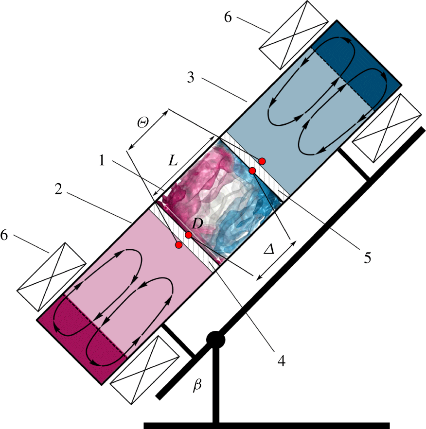
Figure 1. Sketch of the experimental facility, which consists of: (1) a cylindrical convection cell, (2) a hot heat exchanger chamber, (3) a cold heat exchanger chamber, (4) a heated copper plate, (5) a cooled copper plate and (6) inductor coils. The convection cell (1) and heat exchangers (2, 3) are filled with liquid sodium.  $D$ is the diameter and $L$ the length of the cylindrical convection cell (1), $\unicode[STIX]{x1D6FD}$ is the cell inclination angle, $\unicode[STIX]{x1D6E9}$ the temperature drop between the hot and cold heat exchanger chambers, $\unicode[STIX]{x1D6E5}$ the resulting temperature drop between the inner surfaces of the heated and cooled plates of the convection cell (1).
Table 1. The thermal conductivity  $\unicode[STIX]{x1D706}$ and the thermal diffusivity $\unicode[STIX]{x1D705}$ of stainless steel, liquid sodium (Na) and copper (Cu) at the mean temperature of the experiment of approximately 410 K.

Obviously, the boundary conditions in a real liquid–metal experiment and the idealised boundary conditions that are considered in numerical simulations, are different. For example, in the simulations, the cylindrical sidewall is assumed to be adiabatic, while in the real experiment it is made from 3.5 mm thick stainless steel and is additionally covered by a 30 mm thick layer of mineral wool. In table 1, the thermal characteristics of stainless steel, liquid sodium and copper are presented. One can see that the thermal diffusivity of the stainless steel, although being smaller compared to that of liquid sodium, is not negligible. Copper, which is known to be the best material for the heat exchangers in the experiments with moderate or high  $Pr$ fluids, has the thermal diffusivity of the same order as the thermal diffusivity of sodium. Therefore, massive copper plates would not provide a uniform temperature at the surfaces of the plates (Kolesnichenko et al. Reference Kolesnichenko, Mamykin, Pavlinov, Pakholkov, Rogozhkin, Frick, Khalilov and Shepelev2015). To avoid this undesirable inhomogeneity, in our experiment, instead of thick copper plates, we use rather thin ones, which are intensively washed from the outside by liquid sodium of prescribed temperature (see figure 1). The latter process takes place in two heat exchanger chambers, a hot one and a cold one, which are equipped with induction coils. A sodium flow in each heat exchanger chamber is provided by a travelling magnetic field. The induction coils are attached near the outer end faces of the corresponding heat exchanger, thus ensuring that the electromagnetic influence of the inductors on the liquid metal in the convection cell is negligible (Kolesnichenko et al. Reference Kolesnichenko, Khalilov, Teimurazov and Frick2017). Typical velocities of the sodium flows in the heat exchangers are approximately $1~\text{m}~\text{s}^{-1}$, being an order of magnitude higher than the convective velocity inside the convection cell.
In all conducted experiments, the mean temperature of liquid sodium inside the convection cell is approximately  $T_{m}=139.8\,^{\circ }\text{C}$, for which the Prandtl number equals $Pr\approx 0.0093$. Each experiment is performed for a prescribed and known applied temperature difference $\unicode[STIX]{x1D6E9}=T_{hot}-T_{cold}$, where $T_{hot}$ and $T_{cold}$ are the time-averaged temperatures of sodium in, respectively, the hot and cold heat exchanger chambers, which are measured close to the copper plates (see figure 1).
In any hot liquid–metal experiment, there exist unavoidable heat losses due to the high temperature of the set-up. To estimate the corresponding power losses  $Q_{loss}$, one needs to measure additionally the power, which is required to maintain the same mean temperature $T_{m}$ of liquid sodium inside the convection cell, but under the condition of equal temperatures in both heat exchanger chambers, that is, for $\unicode[STIX]{x1D6E9}=0$. From $Q_{loss}$ and the total power consumption $Q$ in the convective experiment at $\unicode[STIX]{x1D6E9}\neq 0$, one calculates the effective power $Q_{eff}=Q-Q_{loss}$ in any particular experiment.
Although the thermal resistance of the two thin copper plates themselves is negligible, the sodium–copper interfaces provide additional effective thermal resistance of the plates mainly due to inevitable oxide films. The temperature drop  $\unicode[STIX]{x1D6E5}_{pl}$ through both copper plates covered by the oxide films could be calculated then from $\unicode[STIX]{x1D6E5}_{pl}=Q_{eff}R_{pl}$, as soon as the effective thermal resistance of the plates, $R_{pl}$, is known. Note that for a fixed mean temperature $T_{m}$, the value of $R_{pl}$ depends on $\unicode[STIX]{x1D6E9}$, since the effective thermal conductivities of the two plates are different due to their different temperatures.
The values of  $R_{pl}(\unicode[STIX]{x1D6E9})$ for different $\unicode[STIX]{x1D6E9}$ are calculated in a series of auxiliary measurements for the case of $\unicode[STIX]{x1D6FD}=0$ and stable temperature stratification, where the heat is applied from above, to suppress convection. In this purely conductive case, the effective thermal resistance of the plates, $R_{pl}$, can be calculated from $\unicode[STIX]{x1D6E9}$ and the measured effective power $\bar{Q}_{eff}$ from the relation $\unicode[STIX]{x1D6E9}=\bar{Q}_{eff}(R_{Na}+R_{pl})$, where the thermal resistance of the liquid sodium equals $R_{Na}=L/(\unicode[STIX]{x1D706}_{Na}S)$ with $\unicode[STIX]{x1D706}_{Na}$ being the liquid-sodium thermal conductivity and $S=\unicode[STIX]{x03C0}R^{2}$ with the cylinder radius $R$.
$R$.
Using the above measured effective thermal resistances of the plates,  $R_{pl}(\unicode[STIX]{x1D6E9})$, in any convection experiment for a given $Ra$ and $\unicode[STIX]{x1D6FD}$ and the mean temperature $T_{m}$, the previously unknown temperature drop $\unicode[STIX]{x1D6E5}$ inside the convection cell can be calculated from $\unicode[STIX]{x1D6E9}$, $R_{pl}(\unicode[STIX]{x1D6E9})$ and measured $Q_{eff}$ as follows:
 $$\begin{eqnarray}\unicode[STIX]{x1D6E5}=\unicode[STIX]{x1D6E9}-\unicode[STIX]{x1D6E5}_{pl},\quad \unicode[STIX]{x1D6E5}_{pl}=Q_{eff}R_{pl}.\end{eqnarray}$$
 Note that in all our measurements in liquid sodium, for all considered inclination angles of the convection cell, the obtained mean temperature and the temperature drop within the cell equal, respectively,  $T_{m}\approx 139.8^{\circ }$ and $\unicode[STIX]{x1D6E5}\approx 25.3~\text{K}$.
The Nusselt number is then calculated as
 $$\begin{eqnarray}Nu=\frac{LQ_{eff}}{\unicode[STIX]{x1D706}_{Na}S\unicode[STIX]{x1D6E5}}.\end{eqnarray}$$
 For a comparison of the experimental results with the DNS and LES results, where the temperatures at the plates inside the convection cell are known a priori, the experimental temperature at the hot plate,  $T_{+}$, and that at the cooled plate, $T_{-}$, are calculated as follows:
 $$\begin{eqnarray}T_{+}=T_{m}+\unicode[STIX]{x1D6E5}/2,\quad T_{-}=T_{m}-\unicode[STIX]{x1D6E5}/2.\end{eqnarray}$$
The Rayleigh number in the experiment is evaluated as
 $$\begin{eqnarray}Ra\equiv \unicode[STIX]{x1D6FC}g\unicode[STIX]{x0394}D^{4}/(L\unicode[STIX]{x1D705}\unicode[STIX]{x1D708}),\end{eqnarray}$$
 which slightly differs from the value defined in (1.1), since  $D$ is slightly smaller than $L$. Thus, for $\unicode[STIX]{x1D6FC}=2.56\times 10^{-4}~\text{K}^{-1}$, $g=9.81~\text{m}~\text{s}^{-2}$, $\unicode[STIX]{x1D6E5}=25.3~\text{K}$, $\unicode[STIX]{x1D708}=6.174\times 10^{-7}~\text{m}^{2}~\text{s}^{-1}$ and $\unicode[STIX]{x1D705}=6.651\times 10^{-5}~\text{m}^{2}~\text{s}^{-1}$, the Rayleigh number equals $Ra=(1.42\pm 0.03)\times 10^{7}$.
For a deep analysis of the convective liquid-sodium flows, the convection cell is equipped with 28 thermocouples, each with an isolated junction of 1 mm. The thermocouples are located on 8 lines aligned parallel to the cylinder axis (see figure 2). The azimuthal locations of these lines are distributed with an equal azimuthal step of  $45^{\circ }$ and are marked in figure 2 by capital letters A to H (counterclockwise, if looking from the cold end face). The line A has the upper position if $\unicode[STIX]{x1D6FD}>0^{\circ }$. On each of the eight lines (A to H), 3 or 5 thermocouples are placed. Thus, all thermocouples are located in five cross-sections of the convection cell, which are parallel to the end faces. The thermocouples are installed inside the convection cell at the same distance of 17 mm from the inner cylinder sidewall and thus are located on five circles, which are marked in figure 2 with numbers $1,\ldots ,5$. The circles 1, 3 and 5 include eight thermocouples, and the circles 2 and 4 only two thermocouples (A and E).
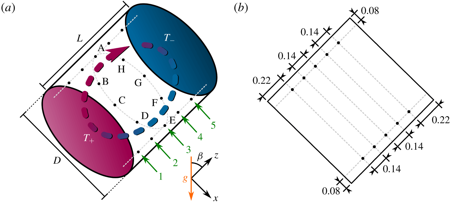
Figure 2. (a) Sketch of an inclined convection cell.  $D$ is the diameter and $L$ the height of the cylindrical sample, $\unicode[STIX]{x1D6FD}$ is the inclination angle, $T_{+}$ ( $T_{-}$) the temperature of the heated (cooled) surfaces. Positioning and naming of the 40 probes inside the cylinder, as considered in the DNS (all combinations of the azimuthal locations A, B, C, D, E, F, G, H and circles $1,\ldots ,5$) and 28 probes in the experiments (all combinations of the eight locations $\text{A},\ldots ,\text{H}$ for the circles 1, 3 and 5 plus four additional probes: A2, A4, E2, E4). Note that the azimuthal locations are shown only for the circle 3, not to overload the sketch. For any inclination angle $\unicode[STIX]{x1D6FD}>0^{\circ }$, the upper azimuthal location is A. (b) Sketch of a central vertical cross-section of the set-up from figure (a), with shown distances (normalised with $L=D$) between the neighbouring probes and between the probes and the sidewall of the cylindrical convection cell.
In this paper, besides the measurements by Khalilov et al. (Reference Khalilov, Kolesnichenko, Pavlinov, Mamykin, Shestakov and Frick2018), where a single Rayleigh number  $Ra=(1.42\pm 0.03)\times 10^{7}$ was considered, we present and analyse also new experimental data, which are obtained for a certain range of the Rayleigh number, based on different imposed temperature gradients.
2.2 Direct numerical simulations
The problem of inclined thermal convection within the Oberbeck–Boussinesq (OB) approximation, which is studied in the DNS, is defined by the following Navier–Stokes, temperature and continuity equations in cylindrical coordinates  $(r,\unicode[STIX]{x1D719},z)$:
 $$\begin{eqnarray}\displaystyle & \displaystyle D_{t}\boldsymbol{u}=\unicode[STIX]{x1D708}\unicode[STIX]{x1D6FB}^{2}\boldsymbol{u}-\unicode[STIX]{x1D735}p+\unicode[STIX]{x1D6FC}g(T-T_{0})\hat{\boldsymbol{e}}, & \displaystyle\end{eqnarray}$$
 $$\begin{eqnarray}\displaystyle & \displaystyle D_{t}T=\unicode[STIX]{x1D705}\unicode[STIX]{x1D6FB}^{2}T, & \displaystyle\end{eqnarray}$$
 $$\begin{eqnarray}\displaystyle & \displaystyle \unicode[STIX]{x1D735}\boldsymbol{\cdot }\boldsymbol{u}=0, & \displaystyle\end{eqnarray}$$
 where  $D_{t}$ denotes the substantial derivative, $\boldsymbol{u}=(u_{r},u_{\unicode[STIX]{x1D719}},u_{z})$ the velocity vector field, with the component $u_{z}$ in the direction $z$, which is orthogonal to the plates, $p$ is the reduced kinetic pressure, $T$ the temperature, $T_{0}=(T_{+}+T_{-})/2$ and $\hat{\boldsymbol{e}}$ is the unit vector, $\hat{\boldsymbol{e}}=(-\text{sin}(\unicode[STIX]{x1D6FD})\cos (\unicode[STIX]{x1D719}),\sin (\unicode[STIX]{x1D6FD})\sin (\unicode[STIX]{x1D719}),\cos (\unicode[STIX]{x1D6FD}))$. Within the considered OB approximation, it is assumed that the fluid properties are independent of the temperature and pressure, apart from the buoyancy term in the Navier–Stokes equation, where the density is taken linearly dependent on the temperature.
These equations are non-dimensionalised by using the cylinder radius  $R$, the free-fall velocity $U_{f}$, the free-fall time $t_{f}$,
 $$\begin{eqnarray}U_{f}\equiv (\unicode[STIX]{x1D6FC}gR\unicode[STIX]{x1D6E5})^{1/2},\quad t_{f}=R(\unicode[STIX]{x1D6FC}gR\unicode[STIX]{x1D6E5})^{-1/2},\end{eqnarray}$$
 and the temperature drop between the heated plate and the cooled plate,  $\unicode[STIX]{x1D6E5}$, as units of length, velocity, time and temperature, respectively.
To close the system (2.5)–(2.7), the following boundary conditions are considered: no slip for the velocity at all boundaries,  $\boldsymbol{u}=0$, constant temperatures ( $T_{-}$ or $T_{+}$) at the face ends of the cylinder and adiabatic boundary condition at the sidewall, $\unicode[STIX]{x2202}T/\unicode[STIX]{x2202}r=0$.
The resulting dimensionless equations are solved numerically with the finite-volume computational code goldfish, which uses high-order interpolation schemes in space and a direct solver for the pressure (Kooij et al. Reference Kooij, Botchev, Frederix, Geurts, Horn, Lohse, van der Poel, Shishkina, Stevens and Verzicco2018). No turbulence model is applied in the simulations. The utilised staggered computational grids of approximately  $1.5\times 10^{8}$ nodes, which are clustered near all rigid walls, are sufficiently fine to resolve the Kolmogorov microscales (see table 2). Statistical averaging is usually carried out for several hundred free-fall time units, which is sufficient not only for integral quantities like the Nusselt number and Reynolds number to converge, but also for the flow fields. The exceptions are the most expensive DNS for liquid sodium. Statistical averaging in our liquid-sodium DNS is, however, the longest known for such low Prandtl numbers and the integral quantities and also the velocity and temperature profiles are converged to a reasonable degree.
Table 2. Details on the conducted DNS and LES, including the time of statistical averaging,  $t_{avg}$, normalised with the free-fall time $t_{f}$; number of nodes $N_{r}$, $N_{\unicode[STIX]{x1D719}}$, $N_{z}$ in the directions $r$,
$r$,  $\unicode[STIX]{x1D719}$ and $z$, respectively; the number of the nodes within the thermal boundary layer, ${\mathcal{N}}_{th}$, and within the viscous boundary layer, ${\mathcal{N}}_{v}$, and the relative thickness of the viscous boundary layer $\unicode[STIX]{x1D6FF}_{u}/L$ (2.17) and the thermal boundary layer $\unicode[STIX]{x1D6FF}_{th}/L$ (2.16).
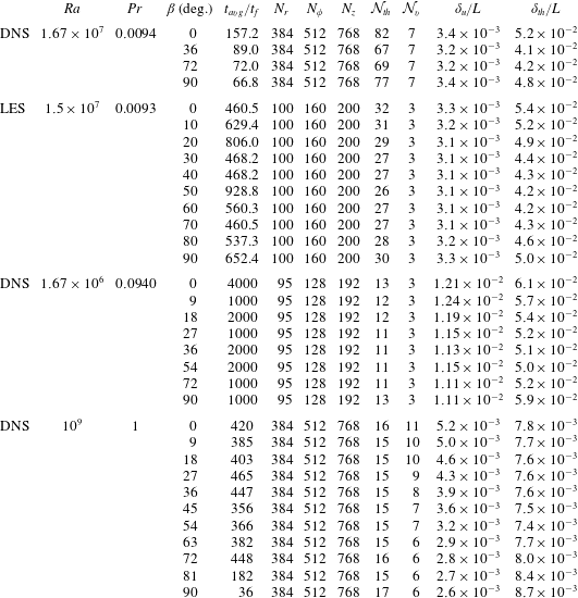
Since simulations on such fine meshes are extremely expensive, only four inclination angles are considered for the main case of  $Pr=0.0094$ and $Ra=1.67\times 10^{7}$, which are $\unicode[STIX]{x1D6FD}=0^{\circ }$, $\unicode[STIX]{x1D6FD}=36^{\circ }$, $\unicode[STIX]{x1D6FD}=72^{\circ }$ and $\unicode[STIX]{x1D6FD}=90^{\circ }$. To study similarities of the flows with respect to the global heat transport and global flow structures for an almost constant Grashof number, $Gr\equiv Ra/Pr$, and for a fixed value of $Ra\,Pr$, some additional DNS of IC were conducted for the combinations of $Pr=0.094$ with $Ra=1.67\times 10^{6}$ and $Pr=1$ with $Ra=10^{9}$. Note that the Grashof number of the auxiliary DNS ( $Gr=10^{9}$) is slightly different from that of the liquid-sodium DNS ( $Gr=1.78\times 10^{9}$). In the former additional DNS, eight different inclination angles are considered, while in the latter additional DNS, 11 different values of $\unicode[STIX]{x1D6FD}$ are examined (see table 2). The computational grids, used in the auxiliary DNS for similar $Ra\,Pr$, contain only three nodes within each viscous boundary layer, however, a convergence study, using twice as many nodes in each direction, for three different inclination angles demonstrated a deviation in $Nu$ and $Ra$ within 1 %.
2.3 Large-eddy simulations
At any fixed time slice, LES generally require more computational effort per computational node, than the DNS. However, since the LES are relieved from the requirement to resolve the spatial Kolmogorov microscales, one can use significantly coarser meshes in the LES compared to those in the DNS, as soon as the LES are verified against the measurements from the physical point of view and against the DNS from the numerical point of view. Thus, the verified LES open the possibility of obtaining reliable data faster, compared to the DNS, using modest computational resources.
In our study, the OB equations (2.5)–(2.7) of thermogravitational convection with the LES approach for small-scale turbulence modelling are solved numerically using the open-source package OpenFOAM 4.1 (Weller et al. Reference Weller, Tabor, Jasak and Fureby1998) for  $Pr=0.0093$ and $Ra=1.5\times 10^{7}$ and 10 different inclination angles, equidistantly distributed between $\unicode[STIX]{x1D6FD}=0^{\circ }$ and $\unicode[STIX]{x1D6FD}=90^{\circ }$.
The package is configured as follows. The used LES model is that by Smagorinsky–Lilly (Deardorff Reference Deardorff1970) with the Smagorinsky constant  $C_{s}=0.17$, which is compatible with the value of the Kolmogorov spectrum constant for the inertial subrange. The turbulent Prandtl number in the core part of the domain equals $Pr_{t}=0.9$ and smoothly vanishes close to the rigid walls. According to different models for liquid metals, the $Pr_{t}$ value can be higher than this one (Chen et al. Reference Chen, Huai, Cai, Li and Meng2013). To estimate the effect of the $Pr_{t}$ value on the simulation results we carried out additional LES with $Pr_{t}$ values up to 4.12 and showed that the specific choice of $Pr_{t}$ does not significantly affect the results. The utilised finite-volume solver is buoyantBoussinesqPimpleFoam with the pressure implicit with splitting of operators (PISO) algorithm by Issa (Reference Issa1986). Time integration is realised with the implicit Euler scheme; the diffusive and convective terms are also treated linearly (more precisely, using the filteredLinear scheme). The resulting systems of linear equations are solved with the preconditioned conjugate gradient method with the diagonal-based incomplete Cholesky preconditioner for the pressure and preconditioned biconjugate gradient method with the diagonal-based incomplete lower–upper (LU) preconditioner for other flow components (Fletcher Reference Fletcher1976; Ferziger & Perić Reference Ferziger and Perić2002).
All simulations are carried out on a collocated non-equidistant computational grid consisting of 2.9 million nodes (see table 2). The grid has a higher density of nodes near the boundaries, in order to resolve the boundary layers. Further details on the numerical method, construction of the computational grid and model verification can be found in Mandrykin & Teimurazov (Reference Mandrykin and Teimurazov2019).
2.4 Methods of data analysis
2.4.1 Nusselt number and Reynolds number
The main response characteristics of the convective system are the global heat and momentum transport represented by the dimensionless Nusselt number  $Nu$ and Reynolds number $Re$, respectively. Within the OB approximation, the Nusselt number equals
 $$\begin{eqnarray}Nu=\langle \unicode[STIX]{x1D6FA}_{z}\rangle _{z},\end{eqnarray}$$
 where  $\unicode[STIX]{x1D6FA}_{z}$ is a component of the heat-flux vector along the cylinder axis:
 $$\begin{eqnarray}\unicode[STIX]{x1D6FA}_{z}\equiv \frac{u_{z}T-\unicode[STIX]{x1D705}\unicode[STIX]{x2202}_{z}T}{\unicode[STIX]{x1D705}\unicode[STIX]{x1D6E5}/L},\end{eqnarray}$$
 and  $\langle \cdot \rangle _{z}$ denotes the average in time and over a cross-section at any distance $z$ from the heated plate.
The Reynolds number can be defined in different ways and one of the common definitions is based on the total kinetic energy of the system
 $$\begin{eqnarray}Re\equiv (L/\unicode[STIX]{x1D708})\sqrt{\langle \boldsymbol{u}\boldsymbol{\cdot }\boldsymbol{ u}\rangle }.\end{eqnarray}$$
 Here,  $\langle \cdot \rangle$ denotes the averaging in time and over the entire volume. We consider also the large-scale Reynolds number
 $$\begin{eqnarray}Re_{U}\equiv (L/\unicode[STIX]{x1D708})\sqrt{\langle \langle \boldsymbol{u}\rangle _{t}^{2}\rangle _{V}},\end{eqnarray}$$
 where  $\langle \cdot \rangle _{t}$ denotes the averaging in time and $\langle \cdot \rangle _{V}$ the averaging over the whole convection cell. Following Teimurazov & Frick (Reference Teimurazov and Frick2017), we also evaluate the Reynolds number based on the volume-averaged velocity fluctuations, or small-scale Reynolds number, as
 $$\begin{eqnarray}Re_{u^{\prime }}\equiv (L/\unicode[STIX]{x1D708})\sqrt{\langle (\boldsymbol{u}-\langle \boldsymbol{u}\rangle _{t})^{2}\rangle }.\end{eqnarray}$$
Finally, one can calculate the Reynolds number based on the ‘wind of turbulence’ as follows:
 $$\begin{eqnarray}Re_{w}=(L/\unicode[STIX]{x1D708})\max _{z}U_{w}(z),\end{eqnarray}$$
where the velocity of the wind, which is parallel to the heated or cooled plates, can be estimated by
 $$\begin{eqnarray}U_{w}(z)=\sqrt{\langle u_{\unicode[STIX]{x1D719}}^{2}+u_{r}^{2}\rangle _{z}},\end{eqnarray}$$
 where  $u_{\unicode[STIX]{x1D719}}$ and $u_{r}$ are the azimuthal and radial components of the velocity, respectively.
In the experiments, the Reynolds number is evaluated based on the average of the estimated axial velocities between the probes along the positions A and E. The velocities are estimated as written below in § 2.4.4.
2.4.2 Boundary-layer thicknesses
Close to the heated and cooled plates, thermal and viscous boundary layers develop. The thickness of the thermal boundary layer is calculated as
 $$\begin{eqnarray}\unicode[STIX]{x1D6FF}_{th}=L/(2Nu).\end{eqnarray}$$
This is the standard way to define the thickness of the thermal boundary layer under the assumption of pure conductive heat transport within this layer, cf. Ahlers et al. (Reference Ahlers, Grossmann and Lohse2009).
Using the slope method (cf. Zhou & Xia Reference Zhou and Xia2010), from the  $U_{w}(z)$ profile along the cylinder axis, see (2.15), the viscous boundary-layer thickness $\unicode[STIX]{x1D6FF}_{u}$ is defined as follows:
 $$\begin{eqnarray}\unicode[STIX]{x1D6FF}_{u}\equiv \max _{z}\{U_{w}(z)\}\left(\left.\frac{\text{d}U_{w}}{\text{d}z}\right|_{z=0}\right)^{-1}.\end{eqnarray}$$
The same criterion was used also for vertical convection before in Ng et al. (Reference Ng, Ooi, Lohse and Chung2015), and can also be adopted to the general case of IC.
2.4.3 Properties of the large-scale circulation
In the DNS and LES, the information on all flow components is available at every small finite volume associated with any grid node. In the experiments, all the information about the flow structures is obtained from the 28 temperature probes located as shown in figure 2 and discussed in § 2.1. The probes are placed in five different horizontal cross-sections of the cylindrical sample, which are parallel to the heated or cooled surfaces. To make a comparison between the DNS, LES and the experiment possible, we measure the temperature and monitor its temporal evolution at the same locations in all three approaches. The only difference is that in the DNS and LES there are eight virtual probes in each cross-section, while in the experiment, there are eight probes in the cross-sections 1, 3 and 5 and only two probes in the cross-sections 2 and 4. The azimuthal locations A to H in the experiment, DNS and LES are exactly the same.
From the temperature measurements at the above discussed locations, one can evaluate the phase and the strength of the so-called wind of turbulence, or large-scale circulation (LSC). To do so, the method by Cioni et al. (Reference Cioni, Ciliberto and Sommeria1997) is applied, which is widely used in RBC experiments (Brown & Ahlers Reference Brown and Ahlers2006; Xi & Xia Reference Xi and Xia2007; Bai, Ji & Brown Reference Bai, Ji and Brown2016; He, Bodenschatz & Ahlers Reference He, Bodenschatz and Ahlers2016; Khalilov et al. Reference Khalilov, Kolesnichenko, Pavlinov, Mamykin, Shestakov and Frick2018) and simulations (Mishra et al. Reference Mishra, De, Verma and Eswaran2011; Stevens, Clercx & Lohse Reference Stevens, Clercx and Lohse2011; Wagner, Shishkina & Wagner Reference Wagner, Shishkina and Wagner2012; Ching, Dung & Shishkina Reference Ching, Dung and Shishkina2017). Thus, the temperature measured at 8 locations in the central cross-section, from A3 to H3 along the central circle 3, is fitted by the cosine function
 $$\begin{eqnarray}T(\unicode[STIX]{x1D703})=T_{m}+\unicode[STIX]{x1D6FF}_{3}\cos (\unicode[STIX]{x1D703}-\unicode[STIX]{x1D703}_{3})\end{eqnarray}$$
 to obtain the orientation of the LSC, represented by the phase  $\unicode[STIX]{x1D703}_{3}$, and the strength of the first temperature mode, i.e. the amplitude $\unicode[STIX]{x1D6FF}_{3}$, which indicates the temperature drop between the opposite sides of the cylinder sidewall. At the warmer part of the sidewall, the LSC carries the warm plumes from the heated plate towards the cold plate and on the opposite colder part, it carries the cold plumes in the opposite direction.
In a similar way one can evaluate the LSC phases  $\unicode[STIX]{x1D703}_{1}$ and $\unicode[STIX]{x1D703}_{5}$ and the strengths $\unicode[STIX]{x1D6FF}_{1}$ and $\unicode[STIX]{x1D6FF}_{5}$ at other heights from the heated plates, i.e. along circle 1 (closer to the heated plate) and along circle 5 (closer to the cooled plate), respectively.
To extract the sloshing mode we use the method by Xi et al. (Reference Xi, Zhou, Zhou, Chan and Xia2009). The so-called temperature extrema extraction (TEE) method is executed as follows: first, the maximum and minimum of the eight probes at a certain time and horizontal level are determined and then a second-order polynomial is fitted exactly through that maximum/minimum using one neighbouring probe to each side (3 points in total per fit). The off-centre distance of the sloshing mode is defined as
 $$\begin{eqnarray}d_{oc}=r_{probes}\cos (\unicode[STIX]{x1D712}),\end{eqnarray}$$
and it measures the shortest distance between the connecting line (of maximum and minimum temperature) and the centreline of the cylinder (cf. figure 3).
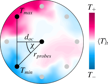
Figure 3. Sketch to illustrate the off-centre distance  $d_{oc}$ of the sloshing mode, as obtained by the temperature extrema extraction method (cf. (2.19)), see Xi et al. (Reference Xi, Zhou, Zhou, Chan and Xia2009).
2.4.4 Velocity estimates
While in the DNS and LES the spatial distributions of all velocity components are available, direct measurements of the velocity in experiments on natural thermal convection in liquid sodium remain impossible so far. In order to estimate the velocities from the temperature measurements in the experiment, the cross-correlations for all combinations of any two neighbouring probes along the azimuthal locations from A to H are used.
For example, the normalised cross-correlation function  $C|_{A1,A2}(\unicode[STIX]{x1D70F})$ for the temporal dependences of the temperatures $T|_{A1}$ and $T|_{A2}$ measured by the probes at the locations A1 and A2 is calculated as follows:
 $$\begin{eqnarray}C|_{A1,A2}(\unicode[STIX]{x1D70F})\propto \mathop{\sum }_{j}(T|_{A1}(t_{j})-\langle T|_{A1}\rangle _{t})\cdot (T|_{A2}(t_{j}+\unicode[STIX]{x1D70F})-\langle T|_{A2}\rangle _{t}).\end{eqnarray}$$
 The first maximum of the function  $C|_{A1,A2}(\unicode[STIX]{x1D70F})$ at $\unicode[STIX]{x1D70F}=\unicode[STIX]{x1D70F}_{c}$ provides the correlation time $\unicode[STIX]{x1D70F}_{c}$. From the known distance between the probes A1 and A2 and the estimated time, $\unicode[STIX]{x1D70F}_{c}$, which is needed for the flow to bring a thermal plume from the location A1 to A2, one can estimate the mean velocity of the flow between the locations A1 and A2.
In a similar way one estimates the mean velocities between the probes A2 and A3, etc., along the azimuthal location A. The mean velocities along the other azimuthal locations, from B to H, are calculated analogously.
3 Results and discussion
In this section, we directly compare the results for inclined convection in a cylindrical container with a diameter-to-height aspect ratio of 1, as they were obtained in the liquid-sodium DNS for  $Ra=1.67\times 10^{7}$ and $Pr=0.0094$, LES for $Ra=1.5\times 10^{7}$ and $Pr=0.0093$ and liquid-sodium experiments for $Ra=1.42\times 10^{7}$ ( $Pr\approx 0.0093$); see tables 3 and 4.
Table 3. Nusselt numbers, as they were obtained in the experiments, DNS and LES. The uncertainty in the experiments is approximately 3 %, in the DNS it is approximately 4 % and IN the LES it is below 1 %.
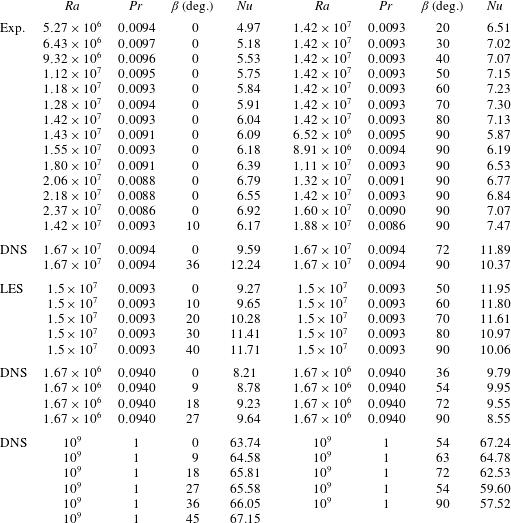
Table 4. Reynolds numbers, a they were obtained in the DNS and LES, see the definitions (2.11), (2.12) and (2.13). The numerical uncertainty of the Reynolds numbers was estimated to be approximately 3 % for DNS and below 1 % for LES.
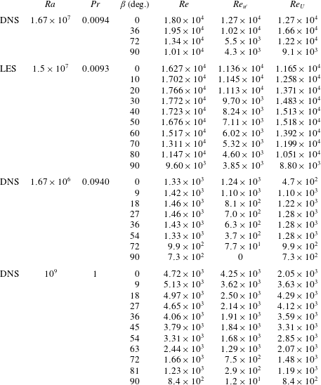
Further liquid-sodium experiments were conducted to measure the scaling relations of the Nusselt number versus the Rayleigh number in the RBC (the inclination angle  $\unicode[STIX]{x1D6FD}=0^{\circ }$) and VC configurations ( $\unicode[STIX]{x1D6FD}=90^{\circ }$), for the $Ra$-range around $Ra=10^{7}$.
Additionally, we make a comparison with the auxiliary DNS results for  $Ra=1.67\times 10^{6}$ and $Pr=0.094$, where the product of the Rayleigh number and Prandtl number, $Ra\,Pr\approx 1.57\times 10^{5}$, is the same as in the main DNS for liquid sodium with $Ra=1.67\times 10^{7}$ and $Pr=0.0094$ (see tables 3 and 4). This auxiliary case is interesting for the following reasons. The ratio of the thermal diffusion time scale, $t_{\unicode[STIX]{x1D705}}=R^{2}/\unicode[STIX]{x1D705}$, to the free-fall time scale, $t_{f}=\sqrt{R/\unicode[STIX]{x1D6FC}g\unicode[STIX]{x1D6E5}}$ is in both cases the same, since $t_{\unicode[STIX]{x1D705}}/t_{f}\sim \sqrt{Ra\,Pr}$. In contrast, in this auxiliary DNS case, the ratio $t_{\unicode[STIX]{x1D708}}/t_{f}$ of the viscous diffusion time scale $t_{\unicode[STIX]{x1D708}}=R^{2}/\unicode[STIX]{x1D708}$ to the free-fall time scale $t_{f}$ is approximately tenfold smaller than that in the main liquid-sodium DNS, albeit being approximately tenfold larger than $t_{\unicode[STIX]{x1D705}}/t_{f}$. Hence, thermal diffusion dominates over viscous diffusion in both considered sets of parameters and for similar $Ra\,Pr$ one might expect similar global temperature distributions and quantitatively similar heat and momentum transport in IC. Note that in the liquid-sodium DNS, the diffusion times are $t_{\unicode[STIX]{x1D705}}\approx 140t_{f}$ and $t_{\unicode[STIX]{x1D708}}\approx 14\,900t_{f}$.
Another set of auxiliary DNS of IC is conducted for  $Ra=10^{9}$ and $Pr=1$ for comparison. In this case, the Grashof number, $Gr\equiv Ra/Pr=10^{9}$, is similar to that in the main liquid-sodium case ( $Gr\approx 1.8\times 10^{9}$), but for this Prandtl-number-one case and the liquid-sodium case we generally do not expect a close similarity of the global flow characteristics.
A summary of the conducted simulations and experiments can be found in table 2. The free-fall time in the experiments equals  $t_{f}=\sqrt{R/(\unicode[STIX]{x1D6FC}g\unicode[STIX]{x1D6E5})}\approx 1.3~\text{s}$ and is similar to that in the main DNS and LES. Thus, the conducted DNS cover only approximately two minutes of the real-time experiment, which was conducted for approximately 7 h. One should note that although the DNS statistical averaging time is quite short, collecting approximately $100t_{f}$ statistics for the case $\unicode[STIX]{x1D6FD}=0^{\circ }$ consumed approximately 390 000 CPUh at the SuperMUC at the Leibniz Supercomputing Centre and required approximately 60 days of runtime.
In the remaining part of this section we investigate integral time-averaged quantities such as the global heat transport (Nusselt number) and the global momentum transport (Reynolds number), provide the evidence of a quantitative agreement between the simulations and experiment and present a complementary picture of the dynamics of the large-scale flows in liquid-sodium IC.
3.1 Time-averaged heat and momentum transport
First, we examine the classical case of RBC without inclination ( $\unicode[STIX]{x1D6FD}=0^{\circ }$). The time-averaged mean heat fluxes, represented by the Nusselt numbers, are presented in figure 4.
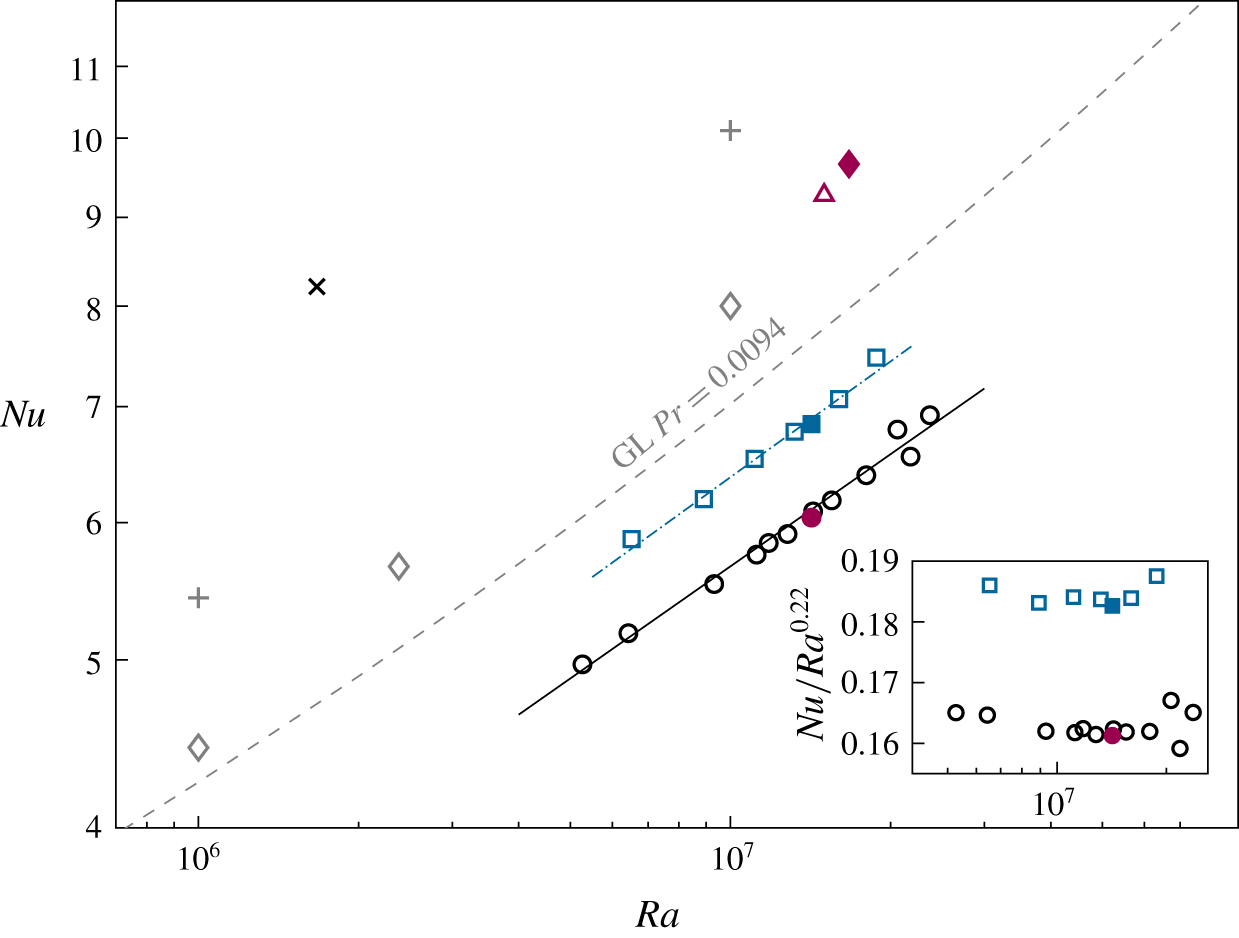
Figure 4. Nusselt number versus Rayleigh number, as obtained in the RBC experiments for different Rayleigh numbers,  $Pr\approx 0.009$, $\unicode[STIX]{x1D6FD}=0^{\circ }$ (open circles) with the effective scaling $Nu\approx 0.177Ra^{0.215}$ (solid line); the RBC experiment for $Ra=1.42\times 10^{7}$, $Pr=0.0093$, $\unicode[STIX]{x1D6FD}=0^{\circ }$ (filled circle; this run is the longest one (7 h) in the series of measurements. For the same $Ra$ and $Pr$, the Nusselt numbers were also measured for different $\unicode[STIX]{x1D6FD}$, see table 3); the VC experiments for different Rayleigh numbers, $Pr\approx 0.009$, $\unicode[STIX]{x1D6FD}=90^{\circ }$ (open squares) with the effective scaling $Nu\approx 0.178Ra^{0.222}$ (dash-dotted line); the inset shows the compensated Nusselt number for RBC and VC experimental data; the DNS for $Ra=1.67\times 10^{7}$, $Pr=0.0094$, $\unicode[STIX]{x1D6FD}=0^{\circ }$ (filled diamond); the DNS for $Ra=1.67\times 10^{6}$, $Pr=0.094$, $\unicode[STIX]{x1D6FD}=0^{\circ }$ (cross); the LES for $Ra=1.5\times 10^{7}$, $Pr=0.0093$, $\unicode[STIX]{x1D6FD}=0^{\circ }$ (open triangle). Results of the RBC DNS by Scheel & Schumacher (Reference Scheel and Schumacher2017) for $Pr=0.005$ (open diamonds) and for $Pr=0.025$ (pluses) and predictions for $Pr=0.0094$ of the Grossmann & Lohse (Reference Grossmann and Lohse2000, Reference Grossmann and Lohse2001) theory considered with the pre-factors from Stevens et al. (Reference Stevens, van der Poel, Grossmann and Lohse2013) (dash line) are presented for comparison. Everywhere a cylindrical convection cell of aspect ratio 1 is considered.
There is an excellent agreement of the DNS and LES data, for example, the Nusselt number deviates less than 1 % and the Reynolds number around 5 % for the RBC and VC cases. Also in figure 4 we compare our numerical results with the DNS by Scheel & Schumacher (Reference Scheel and Schumacher2017), for  $Pr=0.005$ and $Pr=0.025$. Our numerical results for $Pr=0.0094$ and $Pr=0.0093$ take place between the cited results by Scheel & Schumacher (Reference Scheel and Schumacher2017), as expected. Note that our LES and DNS and the DNS by Scheel & Schumacher (Reference Scheel and Schumacher2017) were conducted using completely different codes (the Nek5000 spectral element package in the latter case), but nevertheless lead to consistent results. This verifies to the fact that the obtained results are independent of the numerical method.
The experimental data exhibit generally lower Nusselt numbers (approximately 35 %) compared to the numerical data and this can be explained by the following two reasons. First, the ideal boundary conditions of constant temperatures at the plates cannot be provided in the experiments, since each emission of a sufficiently strong thermal plume affects, at least for a short time, the local temperature at the plate, which results in a reduction of the averaged heat flux compared to that in the simulations with the ideal boundary conditions. Second, the impossibility of measuring the temperature directly at the outer surfaces of the copper plates leads to a slight overestimation of  $\unicode[STIX]{x1D6E9}$ and $\unicode[STIX]{x1D6E5}$ (see figure 1) and, hence, of the effective Rayleigh numbers for the measured Nusselt numbers.
3.1.1 Scaling relations
For  $Pr=0.0094$, the predictions by the Grossmann & Lohse (Reference Grossmann and Lohse2000, Reference Grossmann and Lohse2001) theory, with the prefactors from Stevens et al. (Reference Stevens, van der Poel, Grossmann and Lohse2013), are shown in figure 4 between the obtained experimental and numerical data. The experimental data for a certain $Ra$-range around $Ra=10^{7}$, shown in figure 4, follow a scaling relation
 $$\begin{eqnarray}Nu\approx (0.16\pm 0.01)Ra^{0.22\pm 0.06}\quad (\text{RBC},\,\unicode[STIX]{x1D6FD}=0^{\circ }).\end{eqnarray}$$
 The fitted scaling exponent  $\unicode[STIX]{x1D6FE}$ for the RBC case is smaller than the scaling exponents measured in liquid gallium ( $\unicode[STIX]{x1D6FE}=0.249$, King & Aurnou (Reference King and Aurnou2013)) and liquid mercury ( $\unicode[STIX]{x1D6FE}=0.285$, Takeshita et al. (Reference Takeshita, Segawa, Glazier and Sano1996)). The Prandtl number for both fluids is $Pr\approx 0.025$.
Horanyi et al. (Reference Horanyi, Krebs and Müller1999) measured the heat transport in liquid sodium at  $Pr\approx 0.006$ for $Ra\leqslant 4.5\times 10^{6}$. They used larger aspect ratios from 4.5 to 20, while their highest $Ra$ measurements were conducted in cells with the smallest aspect ratio. Nevertheless, their $Nu\approx 5$ at their highest $Ra\approx 4.5\times 10^{6}$ is similar to $Nu=4.97$ at our lowest $Ra=5.27\times 10^{6}$. Furthermore, Horanyi et al. (Reference Horanyi, Krebs and Müller1999) found that $Nu$ scales as $Ra^{0.25}$, which agrees with our results.
The GL theory predicts a local scaling exponent ranging from 0.23 ( $Ra=5\times 10^{6}$) to 0.26 ( $Ra=3\times 10^{7}$) for $Pr=0.0094$. This results in a mean scaling exponent of approximately 0.25 for this interval of Rayleigh numbers.
We fit  $\log (Nu)$ versus $\log (Ra)$ with a second-order polynomial to estimate the uncertainty of the scaling exponent in our experiments. The local scaling exponent of this fit ranges from 0.16 ( $Ra=5\times 10^{6}$) to 0.27 ( $Ra=3\times 10^{7}$), thus, we estimate the uncertainty of the scaling exponent to be $\unicode[STIX]{x0394}\unicode[STIX]{x1D6FE}=\pm 0.06$. A large variation of the local scaling exponent can be seen in Glazier et al. (Reference Glazier, Segawa, Naert and Sano1999) for liquid mercury in an aspect ratio one cylinder. Their local scaling exponent for small Rayleigh numbers ( ${\sim}10^{6}{-}10^{8}$) is 0.25, while their average scaling exponent is 0.285. Glazier et al. (Reference Glazier, Segawa, Naert and Sano1999) argue that the ‘strong steady bulk mean flow in the cell of aspect ratio one’ reduces the scaling exponent. Presumably, we see a similar effect in our measurements.
In figure 4 we also present the measured scaling relations for  $Nu$ versus $Ra$ for the case of VC ( $\unicode[STIX]{x1D6FD}=90^{\circ }$). The scaling relation in VC is found to be quite similar to that in RBC, namely
 $$\begin{eqnarray}Nu\approx (0.18\pm 0.01)Ra^{0.22\pm 0.06}\quad (\text{VC},\,\unicode[STIX]{x1D6FD}=90^{\circ }).\end{eqnarray}$$
The absolute values of the Nusselt numbers in VC are, however, larger than in RBC.
3.1.2 Time-averaged heat transport in inclined convection
In figure 5(a), the Nusselt numbers in IC are presented, which are normalised by  $Nu$ of the RBC case, for the same $Ra$ and $Pr$, i.e. the dependence of $Nu(\unicode[STIX]{x1D6FD})/Nu(0^{\circ })$ on the inclination angle $\unicode[STIX]{x1D6FD}$. Very remarkable is that, for similar $Ra$ and $Pr$, the DNS and LES deliver very similar values of $Nu$. As previously discussed for the limiting cases (RBC and VC), the deviation between DNS and LES data for the Nusselt numbers is only a few per cent. One can see that the relative increase $Nu(\unicode[STIX]{x1D6FD})/Nu(0^{\circ })$ of the numerical data is up to 10 percentage points higher than that of the experimental data for an inclination angle of approximately $50^{\circ }$. This is accompanied by a shift of the inclination angle with maximal heat transport from approximately $50^{\circ }$ in our numerical results to $70^{\circ }$ in our experimental results. On the one hand, one may take into account that the Rayleigh number in the experiment is slightly smaller ( $Ra=1.42\times 10^{7}$) compared to that in the DNS ( $Ra=1.67\times 10^{7}$) and LES ( $Ra=1.5\times 10^{7}$). On the other hand, the heat transport in the inclined case is enhanced up to 29 % which might reduce the heat loss $Q_{loss}$. However, $Q_{loss}$ is measured in the isothermal case, maintaining the mean temperature in the cylinder (cf. § 2.1). If the heat loss in the inclined case is less than in the isothermal reference case, then also the calculated effective power $Q_{eff}=Q-Q_{loss}$ is lower, and so is the Nusselt number.

Figure 5. (a) Normalised Nusselt number  $Nu(\unicode[STIX]{x1D6FD})/Nu(0^{\circ })$ versus the inclination angle $\unicode[STIX]{x1D6FD}$, as obtained in the DNS for $Ra=1.67\times 10^{7}$, $Pr=0.0094$ (filled diamonds), the LES for $Ra=1.5\times 10^{7}$, $Pr=0.0093$ (open triangles), the DNS for $Ra=1.67\times 10^{6}$, $Pr=0.094$ (crosses), the experiments for $Ra=1.42\times 10^{7}$, $Pr\approx 0.0093$ (open circles) and the DNS for $Ra=10^{9}$, $Pr=1$ (squares). (b) Normalised Reynolds number versus the inclination angle $\unicode[STIX]{x1D6FD}$, as obtained in the same DNS and LES as in (a); similar symbols are used as in (a).
As discussed above, we want to compare our results for liquid sodium with the DNS data for similar  $Ra\,Pr$ and with the DNS data for similar $Ra/Pr$, as in our liquid-sodium measurements and numerical simulations. Figure 5(a) and table 3 show that the obtained Nusselt numbers for the same $Ra\,Pr$ ( $Ra=1.67\times 10^{6}$, $Pr=0.094$) are in good agreement (the difference is less than 10 percentage points) with the liquid-sodium experimental results ( $Ra=1.42\times 10^{7}$, $Pr\approx 0.0093$). Remarkable is that, not only the relative Nusselt number, $Nu(\unicode[STIX]{x1D6FD})/Nu(0^{\circ })$, but also the absolute values of $Nu$ are very similar in the liquid-sodium case and in the case of different $Pr<1$ but the same $Ra\,Pr$. In contrast to that, the $Nu$-dependence on the inclination angle in the case of the same Grashof number is different, as expected. In that case, the maximal relative increase of the Nusselt number due to the cell inclination is only approximately 6 %, while in the liquid-sodium case it is up to 29 %.
3.1.3 Time-averaged momentum transport in inclined convection
In figure 5(b) and table 4, the results for the Reynolds number are presented for the liquid-sodium measurements and simulations as well as for the auxiliary DNS. Again, the agreement between the experiments, DNS and LES for liquid sodium is excellent, usually less than 10 % between DNS and LES. The dependences of  $Re(\unicode[STIX]{x1D6FD})/Re(0^{\circ })$ on the inclination angle, obtained in the liquid-sodium DNS and in the DNS for the same product of $Ra\,Pr$, demonstrate perfect agreement (less than two percentage points difference). The values of $Re(\unicode[STIX]{x1D6FD})/Re(0^{\circ })$ first slightly increase (around 10 %) with the inclination angle and then smoothly decrease, so that the Reynolds number $Re(90^{\circ })$ in the VC case is significantly smaller (only approximately 50 %) than the Reynolds number $Re(0^{\circ })$ in the RBC case. Here one should notice that the absolute values of $Re$ in the liquid-sodium case are significantly larger than in the IC flows for a similar $Ra\,Pr$. In the case of the almost similar Grashof number, the Reynolds numbers decrease much faster with increasing inclination angle than in the liquid-sodium case.
3.1.4 Time-averaged flow structures in inclined convection
Since the Nusselt numbers and relative Reynolds numbers behave very similarly in the liquid-sodium IC experiments and in the DNS for similar  $Ra\,Pr$, we compare the time-averaged flow structures for these cases in figures 6 and 7. In these figures, the time-averaged temperature (figure 6) and the time-averaged component of the heat-flux vector parallel to the cylinder axis $\langle \unicode[STIX]{x1D6FA}_{z}\rangle _{t}$ (figure 7) are presented in the plane of the LSC, for different inclination angles. One can see that both the temperature distributions and the heat-flux distributions, in the liquid-sodium case and in the case of a similar $Ra\,Pr$, look almost identical. In contrast to them, the corresponding distributions for a similar Grashof number look very different. The difference is especially pronounced for the inclination angle $\unicode[STIX]{x1D6FD}=36^{\circ }$. While in the liquid-sodium flow for $\unicode[STIX]{x1D6FD}=36^{\circ }$ there persist two intertwined plumes, a hot one and a cold one, the temperature in the Prandtl-number-one case is better mixed (figure 6) and the heat-flux distribution appears in a form of two triangular-shaped separated spots (figure 7).
From what is presented above, one can see that at almost similar Grashof numbers convection of a Prandtl-number-one fluid leads neither to similar integral quantities like  $Nu$ or $Re$, nor to similar heat flow structures in IC. Thus, it is clearly different to small-Prandtl-number IC flows. In contrast to that, the small-Prandtl-number IC flows of similar $Ra\,Pr$ have similar Nusselt numbers $Nu$, similar relative Reynolds numbers $Re(\unicode[STIX]{x1D6FD})/Re(0^{\circ })$ and similar mean temperature and heat-flux distributions.

Figure 6. Table of vertical slices through the time-averaged temperature in the plane of the LSC, as obtained in the DNS for  $Ra=1.67\times 10^{6}$, $Pr=0.094$ (a,d,g,j); $Ra=1.67\times 10^{7}$, $Pr=0.0094$ (b,e,h,k) and $Ra=10^{9}$, $Pr=1$ (c,f,i,l). From (a) to (l), the inclination angle $\unicode[STIX]{x1D6FD}$ changes from $\unicode[STIX]{x1D6FD}=0^{\circ }$ (RBC case) through $\unicode[STIX]{x1D6FD}=36^{\circ }$ and $\unicode[STIX]{x1D6FD}=72^{\circ }$ to $\unicode[STIX]{x1D6FD}=90^{\circ }$ (VC case).

Figure 7. Table of vertical slices in the plane of the LSC of the time-averaged component of the heat-flux vector parallel to the cylinder axis,  $\langle \unicode[STIX]{x1D6FA}_{z}\rangle _{t}$, normalised by its maximal value through the entire volume, $\unicode[STIX]{x1D6FA}_{max}$, as obtained in the DNS for $Ra=1.67\times 10^{6}$, $Pr=0.094$ (a,d,g,j); $Ra=1.67\times 10^{7}$, $Pr=0.0094$ (b,e,h,k) and $Ra=10^{9}$, $Pr=1$ (c,f,i,l). From (a) to (l), the inclination angle $\unicode[STIX]{x1D6FD}$ changes from $\unicode[STIX]{x1D6FD}=0^{\circ }$ (RBC case) through $\unicode[STIX]{x1D6FD}=36^{\circ }$ and $\unicode[STIX]{x1D6FD}=72^{\circ }$ to $\unicode[STIX]{x1D6FD}=90^{\circ }$ (VC case).
3.2 Temperature and velocity profiles
In this section we analyse the temperature and velocity profiles. The focus thereby is on the following two aspects. First, we compare the experimentally and numerically obtained profiles through the probes (positions A to H) along the lines aligned parallel to the cylinder axes. Second, we compare the velocity profiles, obtained in the DNS and LES, with the velocities evaluated from the correlation times between two neighbouring probes in the experiment, in order to validate the method used in the experiment to estimate the Reynolds number.
In figure 8(a), the time-averaged temperature profiles along the lines of the probe positions A to H are presented for the inclination angles  $\unicode[STIX]{x1D6FD}=36^{\circ }$ (DNS) and $\unicode[STIX]{x1D6FD}=40^{\circ }$ (LES and experiments). Figure 8(b) shows analogous profiles for the inclination angles $\unicode[STIX]{x1D6FD}=72^{\circ }$ (DNS) and $\unicode[STIX]{x1D6FD}=70^{\circ }$ (LES and experiments). In both figures, the profiles at the positions A and E are presented, as well as the average of the profiles at the positions B and H, the average of the profiles at the positions D and F and the average of the C-profile and G-profile. One can see that for the same locations, the LES and DNS profiles are almost indistinguishable, which again demonstrates quantitative agreement between the DNS and LES. The experimental data are available pointwise there, according to the 5 or 3 probes along each location, from A to H. The measurements of the time-averaged temperatures are found to be in good agreement (largest deviation approximately $0.1\unicode[STIX]{x1D6E5}$) with the numerical data, taking into account that the Rayleigh number in the experiments is approximately 15 % smaller than in the DNS.
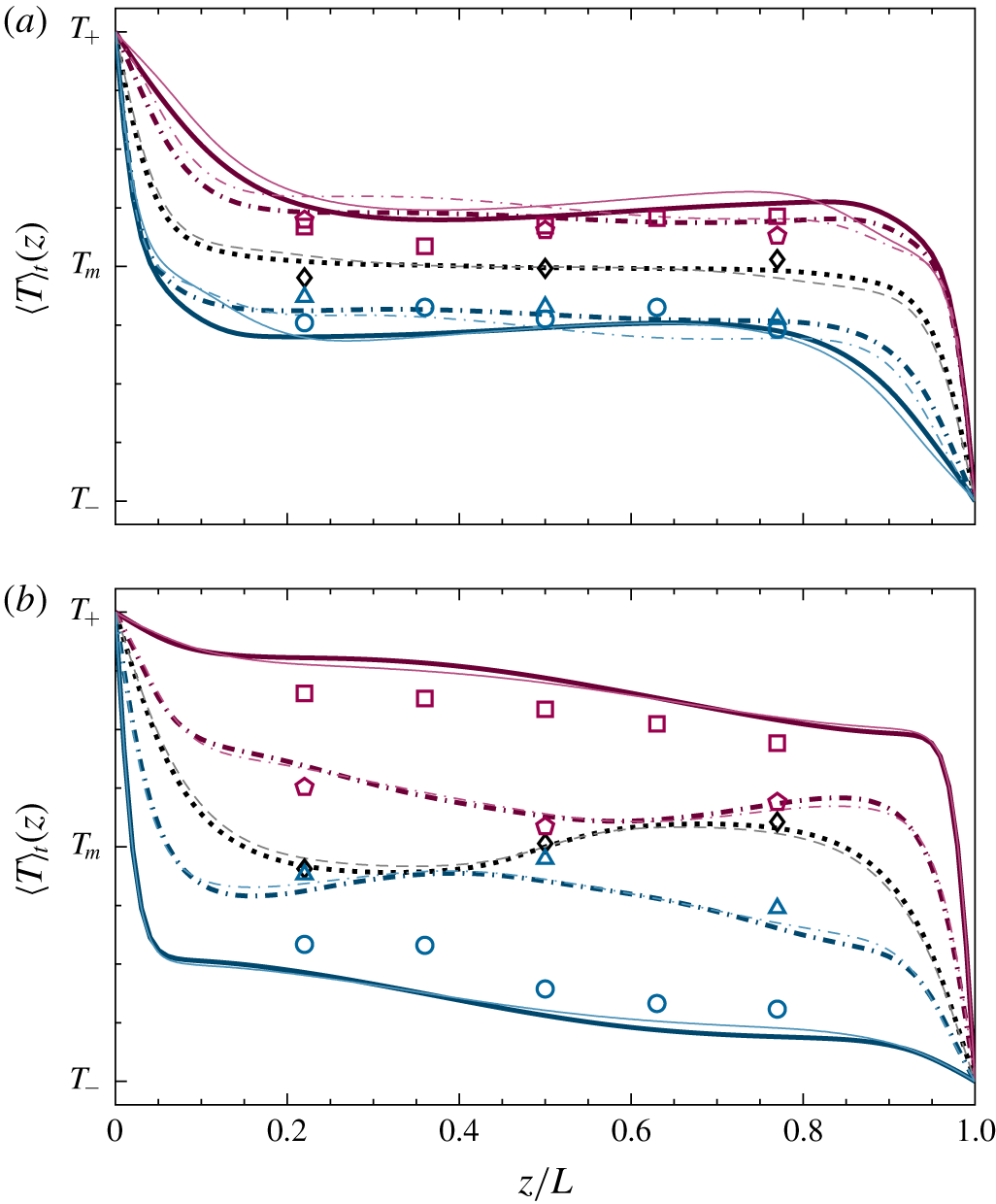
Figure 8. Time-averaged temperature profiles at the positions A to H of the probes, as obtained in (a) the DNS for  $\unicode[STIX]{x1D6FD}=36^{\circ }$ and the LES and experiments for $\unicode[STIX]{x1D6FD}=40^{\circ }$ and in (b) the DNS for $\unicode[STIX]{x1D6FD}=72^{\circ }$ and the LES and experiments for $\unicode[STIX]{x1D6FD}=70^{\circ }$. Thick lines are the DNS data, thin lines are the LES data and symbols are the experimental data. The DNS data are for $Ra=1.67\times 10^{7}$, $Pr=0.0094$, the LES data are for $Ra=1.5\times 10^{7}$, $Pr=0.0093$ and the experiments are for $Ra=1.42\times 10^{7}$, $Pr\approx 0.0093$. Data at the position A (pink solid lines, squares) and the position E (blue solid lines, circles); the average of the data at the positions B and H (pink dash-dotted lines, pentagons), the average of the data at the positions D and F (blue dash-dotted lines, triangles) and the average of the data at the positions C and G (black dotted and grey dash lines, diamonds). The data are averaged along opposite positions due to the expected symmetry and in order to reduce the number of lines in the plot.
At an inclination angle of approximately  $\unicode[STIX]{x1D6FD}=36^{\circ }$ or $\unicode[STIX]{x1D6FD}=40^{\circ }$ (figure 8a), the mean temperature gradient with respect to the direction $z$ across the plates is close to zero in the core part of the domain. This means that the turbulent mixing in this case is very efficient, which is also reflected in the increased Nusselt numbers that we studied before. In contrast to that, for the inclination angle of approximately $\unicode[STIX]{x1D6FD}=70^{\circ }$ (figure 8b), the mean flow is stratified and the temperature profiles have non-vanishing gradients in the $z$-direction.
In figure 9, the time-averaged profiles of the velocity component  $u_{z}$ along the line of the probe positions (A–H) parallel to the cylinder axis are presented for the same inclinations angles, as in figure 8. The velocity estimates at the locations between the neighbouring thermocouples, which are derived from the correlation times obtained in the temperature measurements, are found to be in agreement (largest deviation approximately $0.27U_{f}$) with the DNS and LES data. Thus, this method to estimate the LSC velocity from the temperature measurement is proved to be a very reliable instrument in the IC liquid-sodium experiments.

Figure 9. Time-averaged profiles of the velocity component  $u_{z}$, which is parallel to the cylinder axis, considered at the positions A to H of the probes, as obtained in (a) the DNS for $\unicode[STIX]{x1D6FD}=36^{\circ }$ and the LES and experiments for $\unicode[STIX]{x1D6FD}=40^{\circ }$ and in (b) the DNS for $\unicode[STIX]{x1D6FD}=72^{\circ }$ and the LES and experiments for $\unicode[STIX]{x1D6FD}=70^{\circ }$. Thick lines are the DNS data, thin lines are the LES data and symbols are the experimental data. The DNS data are for $Ra=1.67\times 10^{7}$, $Pr=0.0094$, the LES data are for $Ra=1.5\times 10^{7}$, $Pr=0.0093$ and the experiments are for $Ra=1.42\times 10^{7}$, $Pr\approx 0.0093$. Data at the position A (pink solid lines, squares) and the position E (blue solid lines, circles); the average of the data at the positions B and H (pink dash-dotted lines), the average of the data at the positions D and F (blue dash-dotted lines) and the average of the data at the positions C and G (black dotted and grey dash lines). The data are averaged along opposite positions due to the expected symmetry and in order to reduce the number of lines in the plot.
The viscous boundary-layer thickness ((2.17) and table 2) for the liquid-sodium DNS and LES agree within a small deviation of approximately 3 %. With inclination, the viscous boundary-layer thickness first decreases slightly (by a few per cent) and then gradually increases. Note that the viscous boundary layers defined on the velocity magnitude (Ching et al. Reference Ching, Dung and Shishkina2017) and on the wall shear stress (Scheel & Schumacher Reference Scheel and Schumacher2016) are, respectively, approximately two and three times thicker than the boundary layer defined by (2.17) and table 2.
3.3 Dynamics of the large-scale flow
In this section, we focus on the reconstruction of the rich structural dynamics of the large-scale IC flows in liquid sodium.
It is well known from the previous RBC studies that the LSC in RBC can show different azimuthal orientations (Brown & Ahlers Reference Brown and Ahlers2006; Wagner et al. Reference Wagner, Shishkina and Wagner2012) and can exhibit complicated dynamics with twisting (Funfschilling & Ahlers Reference Funfschilling and Ahlers2004; Funfschilling, Brown & Ahlers Reference Funfschilling, Brown and Ahlers2008; He et al. Reference He, Bodenschatz and Ahlers2016) and sloshing (Xi, Zhou & Xia Reference Xi, Zhou and Xia2006; Xi et al. Reference Xi, Zhou, Zhou, Chan and Xia2009; Brown & Ahlers Reference Brown and Ahlers2009; Zhou et al. Reference Zhou, Xi, Zhou, Sun and Xia2009; Bai et al. Reference Bai, Ji and Brown2016; Zürner et al. Reference Zürner, Schindler, Vogt, Eckert and Schumacher2019). In very-low-Prandtl-number RBC, this complicated behaviour of the LSC was reported in experiments with mercury by Cioni et al. (Reference Cioni, Ciliberto and Sommeria1997) and in the simulations by Schumacher et al. (Reference Schumacher, Bandaru, Pandey and Scheel2016) and Scheel & Schumacher (Reference Scheel and Schumacher2016, Reference Scheel and Schumacher2017).
In our simulations and experiments in liquid sodium, we observe the twisting and sloshing dynamics of the LSC in the RBC configuration of the flow, i.e. without any cell inclination, as well as for small inclination angles  $\unicode[STIX]{x1D6FD}$ until a certain critical $\unicode[STIX]{x1D6FD}=\unicode[STIX]{x1D6FD}_{s}$. The experimental data suggest that a transition to the non-twisting behaviour of the LSC is quite sharp and it is presumably caused by the increasing stratification of the temperature at larger inclination angles (Khalilov et al. Reference Khalilov, Kolesnichenko, Pavlinov, Mamykin, Shestakov and Frick2018).
No LSC cessations were captured in the experiments so far. LSC precession happens only in the RBC case (Khalilov et al. Reference Khalilov, Kolesnichenko, Pavlinov, Mamykin, Shestakov and Frick2018). Only one LSC reversal was captured in a seven-hour-long RBC experiment in liquid sodium (Mamykin et al. Reference Mamykin, Kolesnichenko, Pavlinov and Khalilov2018). Further investigations regarding LSC cessations and reversals need to be carried out in the future.
In figure 10, the time evolution of the volume-averaged components of the heat-flux vector parallel to the cylinder axis,  $\langle \unicode[STIX]{x1D6FA}_{z}\rangle _{V}$ are presented, as they are obtained in the DNS for $Ra=1.67\times 10^{7}$, $Pr=0.0094$ and four different inclination angles between $\unicode[STIX]{x1D6FD}=0^{\circ }$ (RBC) and $\unicode[STIX]{x1D6FD}=90^{\circ }$ (VC). Obviously, in the RBC case, the fluctuations of the heat flux around its mean value are extreme and reach up to $\pm 44\,\%$ of $\langle \unicode[STIX]{x1D6FA}_{z}\rangle$. The strength of the fluctuations gradually decreases with growing inclination angle $\unicode[STIX]{x1D6FD}$ and amount only to $\pm 3\,\%$ of $\langle \unicode[STIX]{x1D6FA}_{z}\rangle$ in the VC case. In figure 10 one can see that for the inclination angles $\unicode[STIX]{x1D6FD}=36^{\circ }$ and $\unicode[STIX]{x1D6FD}=72^{\circ }$, the mean heat transport is stronger than in the RBC or VC cases. This supports a general tendency that in small- $Pr$ fluids the heat transport becomes more efficient, when the convection cell is tilted. Figure 5(a) and table 3 provide a more detailed evidence of this fact, based on our measurements and numerical simulations.

Figure 10. Time dependences of the volume-averaged component of the heat-flux vector along the cylinder axis,  $\langle \unicode[STIX]{x1D6FA}_{z}\rangle _{V}$, as obtained in the DNS for $Ra=1.67\times 10^{7}$, $Pr=0.0094$ and four different inclination angles $\unicode[STIX]{x1D6FD}=0^{\circ }$ (solid line), $\unicode[STIX]{x1D6FD}=36^{\circ }$ (dash line), $\unicode[STIX]{x1D6FD}=72^{\circ }$ (dotted line) and $\unicode[STIX]{x1D6FD}=90^{\circ }$ (dash-dotted line). Time is normalised with $t_{f}=R(\unicode[STIX]{x1D6FC}gR\unicode[STIX]{x1D6E5})^{-1/2}$. The arrows indicate the dimensionless times, which are marked in figure 12 with vertical lines and corresponding 3-dimensional snapshots are shown in figure 13.

Figure 11. Temporal evolution of the phase  $\unicode[STIX]{x1D703}_{1}$ in circle 1 (solid lines) and of the phase $\unicode[STIX]{x1D703}_{5}$ in circle 5 (dash-dotted line) of the convection cell (see locations of the circles in figure 2), as obtained in the experiments for $Ra=1.42\times 10^{7}$, $Pr\approx 0.0093$ (a,c,e,g) and in the DNS for $Ra=1.67\times 10^{7}$, $Pr=0.0094$ (b,d,f,h) for the cell inclination angles $\unicode[STIX]{x1D6FD}=0^{\circ }$ (a,b), $\unicode[STIX]{x1D6FD}=20^{\circ }$ (c), $\unicode[STIX]{x1D6FD}=36^{\circ }$ (d), $\unicode[STIX]{x1D6FD}=40^{\circ }$ (e), $\unicode[STIX]{x1D6FD}=72^{\circ }$ (f) and $\unicode[STIX]{x1D6FD}=90^{\circ }$ (g,h).
3.3.1 The twisting mode
In figure 11 we present the dynamics of the LSC twisting mode. There, the temporal evolution of the phases of the LSC in circle 1 (closer to the heated plate) and in circle 5 (closer to the cold plate) are presented for different inclinations angles  $\unicode[STIX]{x1D6FD}$ of the convection cell filled with liquid sodium, as obtained in our DNS and measurements.
The main evidence for the existence of the twisting mode is the visible strong anti-correlation of the phases  $\unicode[STIX]{x1D703}_{1}(t)$ and $\unicode[STIX]{x1D703}_{5}(t)$, which are measured via the probes at circles 1 and 5, respectively. It is present in the RBC case (figure 11a,b) and for the inclination angles $\unicode[STIX]{x1D6FD}=20^{\circ }$ (figure 11c) and $\unicode[STIX]{x1D6FD}=36^{\circ }$ (figure 11d). The measurements and DNS at the inclination angles $\unicode[STIX]{x1D6FD}\geqslant 40^{\circ }$ (figure 11e) show that, with increasing $\unicode[STIX]{x1D6FD}$, the above anti-correlation vanishes. At large inclination angles, there is no visible anti-correlation of the phases $\unicode[STIX]{x1D703}_{1}(t)$ and $\unicode[STIX]{x1D703}_{5}(t)$ and one can conclude that the twisting movement of the LSC is not present any more (figure 11f,g,h).
The dynamics of the twisting mode of the LSC can be further studied with the Fourier analysis. Thus, from the DNS data ( $Ra=1.67\times 10^{7}$, $Pr=0.0094$) we obtain that the period duration $T_{s}(\unicode[STIX]{x1D6FD})$ equals $T_{s}(0^{\circ })=8.8t_{f}$ for the RBC case and is equal to $T_{s}(36^{\circ })=7.4t_{f}$ for the inclination angle $\unicode[STIX]{x1D6FD}=36^{\circ }$. The experimental data give $T_{s}(0^{\circ })\approx 9.2t_{f}$ for RBC and $T_{s}(20^{\circ })\approx 8.7t_{f}$ for $\unicode[STIX]{x1D6FD}=20^{\circ }$. Note that the frequency $\unicode[STIX]{x1D714}$ of the LSC twisting is approximately proportional to the Reynolds number $\unicode[STIX]{x1D714}\cdot t_{\unicode[STIX]{x1D705}}\sim Re$ (Cioni et al. Reference Cioni, Ciliberto and Sommeria1997). Therefore, the slightly larger period durations in the experiments compared to those in the DNS are consistent with slightly lower Reynolds numbers and Rayleigh numbers there.
We also compare the twisting frequencies obtained in our DNS with results by Schumacher et al. (Reference Schumacher, Bandaru, Pandey and Scheel2016), Xi et al. (Reference Xi, Zhou, Zhou, Chan and Xia2009), Xie, Wei & Xia (Reference Xie, Wei and Xia2013) and Funfschilling & Ahlers (Reference Funfschilling and Ahlers2004). Note that we converted all numbers to free-fall time units ( $t_{f}=R(\unicode[STIX]{x1D6FC}gR\unicode[STIX]{x1D6E5})^{-1/2}$). For low Prandtl numbers, the numerical results by Schumacher et al. (Reference Schumacher, Bandaru, Pandey and Scheel2016) give a period of $4.6t_{f}$ for $Pr=0.021$ and $Ra=10^{7}$. At higher Prandtl numbers the period is much longer. For water it is approximately $30t_{f}$ at $Pr=5.3$ and $Ra=5\times 10^{9}$ (Xi et al. Reference Xi, Zhou, Zhou, Chan and Xia2009). For even lager Prandtl number, $Pr=19.4$, Xie et al. (Reference Xie, Wei and Xia2013) found $T_{s}\approx 85t_{f}$ at $Ra=2\times 10^{11}$. The twisting frequency is lower with increasing $Pr$ at high Prandtl numbers ( $Pr>1$). However, the twisting frequency is slightly lower at $Pr=0.0094$ compared to $Pr=0.021$ for similar Rayleigh number.
3.3.2 The sloshing mode
Besides the twisting mode there is another mode present in the flow. This is the sloshing mode; it brings together the hot and cold streams of the LSC. Both the twisting and the sloshing mode are observed simultaneously, and the full LSC dynamics is determined by a combination of both modes. To quantify the sloshing motion, we calculate the off-centre distance (2.19) and plot it over time (figure 12c) for the example case (DNS,  $Ra=1.67\times 10^{7}$, $Pr=0.0094$, $\unicode[STIX]{x1D6FD}=36^{\circ }$). The sloshing mode has the same frequency as the twisting mode (correlation of both signals is ${>}0.8$), but it shows a phase difference of approximately $\frac{1}{4}$-period. From the comparison of $d_{oc}(t)$ and $\langle \unicode[STIX]{x1D6FA}_{z}\rangle _{V}(t)$ we learn that, first the hot and cold streams are brought close to each other, and then, with a short delay, the heat transport increases.
The sloshing mode is coherent through the entire height of the cylinder, quantified by a correlation of at least 0.8 between the sloshing signal ( $d_{oc}$) at mid-height circle 3 and the lower/higher circles (1, 2, 4 and 5). The correlation of circles 1 and 5 is approximately 0.75.

Figure 12. Temporal evolution of different quantities obtained in the DNS for  $Ra=1.67\times 10^{7}$, $Pr=0.0094$ and the cell inclination angle $\unicode[STIX]{x1D6FD}=36^{\circ }$: (a) the temperature $T$ at the probes B3 (solid line), D3 (dash-dotted line), F3 (dotted line) and H3 (dash line); (b) the phase $\unicode[STIX]{x1D703}_{1}$ in circle 1 (solid line) and the phase $\unicode[STIX]{x1D703}_{5}$ in circle 5 (dash-dotted line) and (c) the volume-averaged component of the heat-flux vector along the cylinder axis, $\langle \unicode[STIX]{x1D6FA}_{z}\rangle _{V}$ (solid line) and the off-centre distance, $d_{oc}$ (dashed line). The three vertical lines mark the times at which the snapshots in figure 13 are taken. The phases $\unicode[STIX]{x1D703}_{1}(t)$ and $\unicode[STIX]{x1D703}_{5}(t)$ in (b) have a period of $T_{\unicode[STIX]{x1D703}}=(7.4\pm 0.2)t_{f}$, which is determined by the Fourier analysis.

Figure 13. Three-dimensional side views (a,d,g) and views orthogonal to the side views and to the cylinder axis (b,e,h) of the temperature isosurfaces and the corresponding horizontal slices at the mid-height of the instantaneous temperature fields as seen from the cold plate (c,f,i), which are obtained in the DNS for  $Ra=1.67\times 10^{7}$, $Pr=0.0094$ and the cell inclination angle $\unicode[STIX]{x1D6FD}=36^{\circ }$ at the times (a,b,c) $t=17t_{f}$, (d,e,f) $t=19t_{f}$, (g,h,i) $t=21t_{f}$. The dot (green online) marks the location A3. The snapshots presented here correspond to the times marked in figure 12 with the vertical lines.
Let us investigate the IC flow in liquid sodium for the inclination angle  $\unicode[STIX]{x1D6FD}=36^{\circ }$, as in figure 11(d), where a very strong LSC twisting is observed. In figure 12 we analyse this flow in more detail. Figure 12(a) presents the evolution of the temperature in time, which is measured by the probes B3, D3, F3 and H3 that are placed in the central circle 3.
One can see that the temperature dependencies on time at the locations B3 and F3 are synchronous. So are the temperature dependencies on time at the locations H3 and D3. The temperatures at the locations B3 and D3 are anti-correlated. So are the temperatures at the locations H3 and F3. Thus, when at the location B3 the fluid is extremely hot, the lowest temperature is obtained near D3, which is located only  $90^{\circ }$ azimuthally below B3. Analogously, when the fluid is hot at the location H3, its lowest temperature is obtained near the location F3, which is $90^{\circ }$ below H3 (see also figure 13). These events happen at the times $t/t_{f}=17$ and $t/t_{f}=21$ in figure 12, respectively. Thus, at the times $t/t_{f}=17$ and $t/t_{f}=21$ a big hot and a big cold plume approach each other very closely. This sloshing movement happens periodically, alternately, near one side of the sidewall, then on the opposite side.
Figure 12(b) presents the evolution in time of the LSC phase  $\unicode[STIX]{x1D703}_{1}$ in circle 1 (close to the heated plate) and of the phase $\unicode[STIX]{x1D703}_{5}$ in circle 5 (close to the cold plate).
These phases are anti-correlated, and the twisting of the LSC near the plates is maximal (at  $t/t_{f}=19$) when the hot and the cold streams of the LSC in the central cross-section are located near the opposite sides of the cylinder sidewall.
In figure 12(c) the temporal evolution of the volume-averaged heat-flux vector parallel to the cylinder axis,  $\langle \unicode[STIX]{x1D6FA}_{z}\rangle _{V}$, is presented. Again, a very strong relationship with the LSC twisting and sloshing is observed. The maximal values of $\langle \unicode[STIX]{x1D6FA}_{z}\rangle _{V}$ are obtained when the hot and cold LSC streams meet, thanks to sloshing, while the minimum value is obtained at the time periods when the LSC is strongly twisted.
In figure 13, the above described process, namely, the azimuthal movement of the hot and cold batches of fluid in the form of an oscillatory motion against each other, is illustrated with three-dimensional side views in two perpendicular directions. Additionally, the corresponding horizontal cross-sections of the instantaneous temperature fields at the mid-height of the cylinder are presented there. In the supplementary movies to this paper, available at https://doi.org/10.1017/jfm.2019.935, the described dynamics of the LSC can be observed in detail.
3.3.3 Statistics of the large-scale circulation
In figure 14(a) the standard deviations of the phases  $\unicode[STIX]{x1D703}_{i}$ in the circles $i=1$, 3 and 5 are presented, while figure 14(b) shows the corresponding time-averaged strengths of the LSC, $\langle \unicode[STIX]{x1D6FF}_{i}\rangle _{t}$, as they are obtained in the liquid-sodium measurements and DNS. The measurements show that the standard deviations of the phases $\unicode[STIX]{x1D703}_{1}$ (near the heated plate) and $\unicode[STIX]{x1D703}_{5}$ (near the cooled plate) are relatively large for small inclination angles, while being small for large inclination angles. There exist almost immediate drops of $\unicode[STIX]{x1D703}_{1}(\unicode[STIX]{x1D6FD})$ and $\unicode[STIX]{x1D703}_{5}(\unicode[STIX]{x1D6FD})$ that happen between $\unicode[STIX]{x1D6FD}=20^{\circ }$ and $\unicode[STIX]{x1D6FD}=40^{\circ }$, which indicate a sharp transition between the twisting and sloshing modes of the LSC and the usual mode of the LSC, when it is not twisted and located basically in the central vertical cross-section along the axis of the cylindrical sample. The standard deviations of $\unicode[STIX]{x1D703}_{1}$, $\unicode[STIX]{x1D703}_{3}$ and $\unicode[STIX]{x1D703}_{5}$, obtained in the DNS, show generally a similar behaviour as those measured in the experiments, but due to only a few considered inclination angles in the DNS, it is impossible to resolve the sudden drop which is observed in the measurements. Also one should notice that the data in figure 14 are very sensitive to the time of statistical averaging, which is extremely short in the DNS compared to the experiment.

Figure 14. (a) Standard deviations of the phase angles  $\unicode[STIX]{x1D703}_{i}$ in radians normalised by $2\unicode[STIX]{x03C0}$ and (b) the time-averaged strengths of the large-scale circulation, $\langle \unicode[STIX]{x1D6FF}_{i}\rangle _{t}$, as obtained at the probe circle 1 (pink colour symbols and lines), circle 3 (grey colour) and circle 5 (blue colour) in the experiments (dash-dotted lines), the DNS for $Ra=1.67\times 10^{7}$, $Pr=0.0094$ (solid lines) and DNS for $Ra=10^{6}$, $Pr=0.094$ (dash lines).
The results for the time-averaged strengths of the LSC,  $\langle \unicode[STIX]{x1D6FF}_{i}\rangle _{t}$, obtained in the measurements and DNS (figure 14b) show similar trends. In the RBC case ( $\unicode[STIX]{x1D6FD}=0^{\circ }$), the LSC strength is small and grows smoothly with the inclination angle $\unicode[STIX]{x1D6FD}$. However, the mean strength of the LSC in the measurements is approximately $0.02\unicode[STIX]{x1D6E5}$, i.e. 2 % of the temperature difference, weaker that the one in the liquid-sodium DNS. This is consistent with the lower Nusselt number, as well as the lower Rayleigh number of the experiments. Surprisingly, the liquid-sodium DNS data show a similar strength of the LSC as the data from the auxiliary DNS for the same $Ra\,Pr$.
Table 5. Uncertainties  $\unicode[STIX]{x1D703}_{err}=|\unicode[STIX]{x1D703}^{(n)}-\unicode[STIX]{x1D703}^{(512)}|$ and $\unicode[STIX]{x1D6FF}_{err}=|\unicode[STIX]{x1D6FF}^{(n)}/\unicode[STIX]{x1D6FF}^{(512)}-1.|$ that are caused by the limited number of probes $n$ while using the cos method to determine the phase $\unicode[STIX]{x1D703}_{i}$ and strength $\unicode[STIX]{x1D6FF}_{i}$ of the LSC. All values are averaged over 5 circles and 400 snapshots of the DNS data for $Ra=1.67\times 10^{7}$, $Pr=0.0094$, $\unicode[STIX]{x1D6FD}=0^{\circ }$.
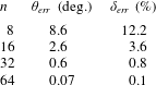
Evaluating the LSC phase angle  $\unicode[STIX]{x1D703}_{i}$ and strength $\unicode[STIX]{x1D6FF}_{i}$ using the cos method (Cioni et al. Reference Cioni, Ciliberto and Sommeria1997) by fitting only eight probes results in an uncertainty of approximately $8.6^{\circ }$ and 12.2 %, respectively. In table 5 we compare the mean deviation of the fit with a given number of probes $n$ compared to the case $n=512$. We find that the use of 32 probes is sufficient to reduce the uncertainty to below $1^{\circ }$ and 1 %, respectively. However, using only eight probes in the experiment is acceptable, especially considering that every additional probe disturbs the flow.
4 Conclusions
In our complementary and cross-validating experimental and numerical studies, we have investigated inclined turbulent thermal convection in liquid sodium ( $Pr\approx 0.009$) in a cylindrical container of aspect ratio one. The results of the conducted measurements, DNS and LES demonstrated a good quantitative agreement, and the uncertainty margin has been extensively discussed.
For the limiting cases of inclined convection, which are Rayleigh–Bénard convection (with the cell inclination angle  $\unicode[STIX]{x1D6FD}=0^{\circ }$) and vertical convection ( $\unicode[STIX]{x1D6FD}=90^{\circ }$), we have experimentally studied the scaling relations of the mean heat flux (Nusselt number) with Rayleigh number, for $Ra$ around $10^{7}$. The scaling exponents were found to be approximately 0.22 in both cases, but the absolute values of $Nu$ are found to be larger in VC, compared to those in RBC. At the considered Rayleigh number of approximately $1.5\times 10^{7}$, any inclination of the RBC cell generally leads to an increase of the mean heat flux. The maximal $Nu$ is obtained, however, for a certain intermediate value of $\unicode[STIX]{x1D6FD}$ and may increase up to 29 % (compared to the RBC case) for liquid sodium at the considered Rayleigh number.
It was proved, in particular, that the use of the cross-correlation time of the neighbouring temperature probes is a reliable tool to evaluate velocities during temperature measurements in liquid sodium.
We showed (cf. table 5) that, using the cos method (2.18) to determine the phase  $\unicode[STIX]{x1D703}_{i}$ and strength $\unicode[STIX]{x1D6FF}_{i}$ of the LSC with only 8 probes, one obtains reliable results with an uncertainty of approximately $8.6^{\circ }$ and $\pm 12.2\,\%$, respectively.
Furthermore, we have found that for small Prandtl numbers there exists a similarity of IC flows of the same  $Ra\,Pr$, due to the similar ratio, $t_{\unicode[STIX]{x1D705}}/t_{f}\sim \sqrt{RaPr}$, between the thermal diffusion time scale, $t_{\unicode[STIX]{x1D705}}$, and the free-fall time scale, $t_{f}$. Since in small- $Pr$ convective flows, the viscous diffusion time scale, $t_{\unicode[STIX]{x1D708}}$, is much larger than $t_{\unicode[STIX]{x1D705}}$, the value of $Ra\,Pr$ determines basically the mean temperature and heat-flux distributions. The Nusselt numbers and the relative Reynolds numbers of the liquid-sodium DNS and auxiliary DNS at similar $Ra\,Pr$ are similar for any inclination of the convection cell with respect to the gravity vector. This property can be very useful for the investigation of, e.g., the scaling relations of $Nu$ and $Re$ with $Ra$ and $Pr$ or of the mean temperature or heat-flux distributions, at extremely high $Ra$ and/or extremely small $Pr$.
$Pr$.
For small inclination angles, the large-scale circulation exhibits complex dynamics, with twisting and sloshing modes and these modes strongly influence the instantaneous heat transport in the system ( $\pm 44\,\%$ of the mean heat transport). In a strongly twisted LSC, the volume-averaged vertical heat flux is minimal, and it is maximal, shortly after the LSC sloshing mode brought together the hot and cold streams of the LSC. Note that both modes are present in the flow simultaneously. Figures 12 and 13 and supplementary movies illustrate the studied LSC dynamics. Additional investigations will be needed to study the even more complex behaviour of the LSC in IC of low- $Pr$ fluids in elongated containers with $L\gg D$.
Acknowledgements
This work is supported by the Priority Programme SPP 1881 Turbulent Superstructures of the Deutsche Forschungsgemeinschaft (DFG) under the grant Sh405/7. O.S. also thanks the DFG for the support under the grant Sh405/4 – Heisenberg fellowship. The authors acknowledge the Leibniz Supercomputing Centre (LRZ) for providing computing time and the Institute of Continuous Media Mechanics (ICMM UB RAS) for providing resources of the Triton supercomputer.
Supplementary movies
Supplementary movies are available at https://doi.org/10.1017/jfm.2019.935.


 Open access