


1. Introduction
Understanding the dynamics of concentrated suspensions of soft, athermal particles such as emulsions, foams or gels is key to many natural and industrial processes (Larson Reference Larson1999; Coussot Reference Coussot2005; McClements Reference McClements2015). A central question concerns the connection between mechanisms occurring at the microstructure level and the macroscopic flow and rheological properties in these systems (Cohen-Addad, Hohler & Pitois Reference Cohen-Addad, Hohler and Pitois2013; Dollet & Christophe Reference Dollet and Christophe2014; Bonn et al. Reference Bonn, Denn, Berthier, Divoux and Manneville2017; Dijksman Reference Dijksman2019). For instance, irreversible topological rearrangements, corresponding to local yielding events, are known to be directly related to the inhomogeneous fluidisation of soft glassy materials (Goyon et al. Reference Goyon, Colin, Ovarlez, Ajdari and Bocquet2008; Bocquet, Colin & Ajdari Reference Bocquet, Colin and Ajdari2009; Bouzid et al. Reference Bouzid, Izzet, Trulsson, Clément, Caludin and Andreotti2015; Dollet, Scagliarini & Sbragaglia Reference Dollet, Scagliarini and Sbragaglia2015; Fei et al. Reference Fei, Scagliarini, Luo and Succi2020). Fostered by such rheological implications, but going beyond them, many experimental and numerical studies have been devoted to characterising the microdynamics of soft jammed materials by tracking individual mesoconstituents (droplets, bubbles, grains, etc.), unveiling their anomalous dispersion properties (Durian, Weitz & Pine Reference Durian, Weitz and Pine1991; Durian Reference Durian1995; Lowenberg & Hinch Reference Lowenberg and Hinch1996; Mason et al. Reference Mason, Ganesan, van Zanten, Wirtz and Kuo1997; Cipelletti et al. Reference Cipelletti, Ramos, Manley, Pitard, Weitz, Pashkovski and Johansson2003; Ruzicka, Zulian & Ruocco Reference Ruzicka, Zulian and Ruocco2004; Cerbino & Trappe Reference Cerbino and Trappe2008; Squires & Mason Reference Squires and Mason2010). Looking at the droplet statistical dynamics from a Lagrangian viewpoint is, therefore, crucial. Highly packed emulsions/foams are typically characterised in simple flows (oscillatory Couette, Poiseuille, etc.), or even at rest, in the ageing regime (Mason & Weitz Reference Mason and Weitz1995; Ramos & Cipelletti Reference Ramos and Cipelletti2001; Cipelletti et al. Reference Cipelletti, Ramos, Manley, Pitard, Weitz, Pashkovski and Johansson2003; Cipelletti & Ramos Reference Cipelletti and Ramos2005; Li, Peng & McKenna Reference Li, Peng and McKenna2019; Giavazzi, Trappe & Cerbino Reference Giavazzi, Trappe and Cerbino2021). On the other hand, Lagrangian studies of dispersions in complex, high Reynolds number flows are widely represented in the literature, but in extremely diluted conditions (Toschi & Bodenschatz Reference Toschi and Bodenschatz2009; Brandt & Coletti Reference Brandt and Coletti2022). The investigation of the microdynamics of concentrated systems in complex flows, of relevance, e.g. for emulsification processes (Tcholakova et al. Reference Tcholakova, Vankova, Denkov and Danner2007; Vankova et al. Reference Vankova, Tcholakova, Denkov, Ivanov, Vulchev and Danner2007a,Reference Vankova, Tcholakova, Denkov, Vulchev and Dannerb), is, in fact, a formidable task due to the need to cope, at the same time, with the two-way coupling of the interfacial dynamics with the hydrodynamics and with the droplet/bubble tracking.
Motivated by the above discussion, in the present paper we aim at investigating the statistical dynamics of emulsion droplets in a systematic way across various concentrations (from semi-dilute to jammed conditions), under the action of a large-scale forcing, inducing a chaotic, turbulent-like flow, and during ageing. For our purpose, we employ a mesoscopic numerical model, developed over the last 15 years, to simulate the hydrodynamics of three-dimensional immiscible fluid mixtures, stabilised against full phase separation, equipped with a droplet tracking algorithm. The same approach was used in a recent publication (Girotto et al. Reference Girotto, Benzi, Di Staso, Scagliarini, Schifano and Toschi2022) to show how to prepare an emulsion, by means of a suitable combination of stirring and injection of the dispersed phase, and how to characterise it both structurally and rheologically: structurally, by looking at the evolution of the droplet size distribution, which we found to be in close agreement with known experimental results; rheologically, by looking at the emergence of the yield stress for large enough volume fractions,  $\phi$. In Girotto et al. (Reference Girotto, Benzi, Di Staso, Scagliarini, Schifano and Toschi2022), we also showed that, for a given amplitude of the large-scale stirring, upon increasing the volume fraction $\phi$ of the disperse phase, there exists a critical value $\phi _{cpi}$ at which a sudden catastrophic phase inversion occurs (Bouchama et al. Reference Bouchama, van Aken, Autin and Koper2003; Perazzo, Preziosi & Guido Reference Perazzo, Preziosi and Guido2015) (see figure 5 in Girotto et al. Reference Girotto, Benzi, Di Staso, Scagliarini, Schifano and Toschi2022).
At low volume fractions droplets are normally far from each other and regularly collide due to the presence of the flow; elastoplastic rearrangements are not defined in this regime. For high volume fractions ( ${\gtrsim }60\,\%$), on the contrary, droplets are mostly in contact with each other and the emulsion regularly undergoes elastoplastic rearrangements; it is not possible to properly talk of collisions in this case as the droplets are always in contact. For a small range of intermediate volume fractions, one could observe both collisions and elastoplastic rearrangements; in this regime it is, however, very hard to define whether or not droplets are in contact with each other and therefore to clearly distinguish between a flow-induced collision or an elastoplastic rearrangement. Here, we provide measurements of droplet absolute (single) and relative (pair) dispersions, velocity and acceleration distributions, as well as of the droplet breakup, $\beta$, and coalescence, $\kappa$, rates. An interesting, and we feel important, result of our investigation is that $\beta$, $\kappa$ and the average droplet size shows divergent-like behaviour for $\phi \rightarrow \phi _{cpi}$, which is consistent (in the language of statistical mechanics) with the identification of $\phi _{cpi}$ as a critical point of a phase transition. Also, upon increasing $\phi$ from a semi-dilute to a highly concentrated emulsion, droplet accelerations show increasingly intermittent features due to increasing stiffness and elastoplastic effects in the system. For large enough volume fraction, we also studied the so-called ageing regime, i.e. we stop the forcing and we look at the droplet dynamics. Remarkably, droplet dispersion and pair separation (here studied for the first time) show a ballistic regime followed by a clear superdiffusive behaviour. For pair dispersion in the ageing regime we propose theoretical models that show good agreement with the measurements.
The paper is organised as follows. In § 2 we present the numerical method and we provide an extensive introduction to the tracking algorithm. The main results are reported in § 3, organised in subsections relative to the stirred and ageing regimes. Conclusions and perspectives are drawn in § 4.
2. Methods
2.1. Multicomponent emulsion modelling
The emulsion is described in terms of the density fields of the two components, conventionally indicated as  $O$ and $W$ (for, e.g. ‘oil’ and ‘water’), $\rho _{O,W}$, and the incompressible barycentric fluid velocity field, $\boldsymbol {u}$, which evolve according to the following equations:
 \begin{equation} \left.\begin{gathered} \partial_t \rho_{\sigma} + \boldsymbol{\nabla}\boldsymbol{\cdot}(\rho_{\sigma}\boldsymbol{u}) = 0 \quad \sigma = O,W \\ \rho_f (\partial_t \boldsymbol{u} + \boldsymbol{u} \boldsymbol{\cdot}\boldsymbol{\nabla}\boldsymbol{u}) =- \boldsymbol{\nabla} p + \boldsymbol{\nabla}\boldsymbol{\cdot} \boldsymbol{P}^{{(mix)}} + \eta \nabla^2 \boldsymbol{u} + \boldsymbol{F}^{({ext})}, \end{gathered}\right\} \end{equation}
where  $\rho _f = \rho _O + \rho _W$ is the total density, $p$ is the pressure, $\eta$ is the dynamic viscosity and $\boldsymbol {F}^{({ext})}$ a forcing term; $P^{({mix})}_{ij}[\rho _O, \rho _W, \partial _i \rho _O, \partial _i \rho _W,\dots ]$, a function of the two density fields and of their derivatives, is the non-ideal contribution to the pressure tensor. Equations (2.1) are integrated numerically on a three-dimensional (3-D) cubic domain of size $L^3$ with periodic boundary conditions by means of a two-component lattice Boltzmann method (Benzi, Succi & Vergassola Reference Benzi, Succi and Vergassola1992) in the Shan–Chen formulation (Shan & Chen Reference Shan and Chen1993, Reference Shan and Chen1994). The lattice Boltzmann equation for the discrete probability distribution functions, $f_{\sigma l}$, reads (the time step is set to unity, $\varDelta = 1$)
 \begin{equation} f_{\sigma l}(\boldsymbol{x}+\boldsymbol{e}_l, t + 1) - f_{\sigma l}(\boldsymbol{x}, t) =-\frac{1}{\tau_{\sigma}}\left(f_{\sigma l}(\boldsymbol{x}, t) - f_{\sigma l}^{eq}(\boldsymbol{x}, t) \right) + S^{{(tot)}}_{\sigma l}(\boldsymbol{x}, t), \end{equation}
where the index  $l$ runs over the discrete set of $Q=19$ 3-D lattice velocities ( $D3Q19$ model) $\{\boldsymbol {e}_l\}$ ( $l=0,1,\dots,18$), and $\sigma$ labels each of the two immiscible fluids (hereafter, we take the same relaxation time for the two species, i.e. $\tau _O = \tau _W \equiv \tau$). The equilibrium distribution function is given by the usual polynomial expansion of the Maxwell–Boltzmann distribution, valid in the limit of small fluid velocity, namely
 \begin{equation} f_{\sigma l}^{eq}(\boldsymbol{x}, t) = \rho_{\sigma}\omega_l\left(1 + \frac{\boldsymbol{e}_l\boldsymbol{\cdot}\boldsymbol{u}}{c^2_s} + \frac{(\boldsymbol{e}_l\boldsymbol{\cdot}\boldsymbol{u})^2}{2c_s^4} - \frac{\boldsymbol{u}\boldsymbol{\cdot}\boldsymbol{u}}{2c^2_s} \right), \end{equation}
with  $\omega _l$ being the usual set of suitably chosen weights so as to maximise the algebraic degree of precision in the computation of the hydrodynamic fields and $c_s=1/\sqrt {3}$ a characteristic molecular velocity (a constant of the model). The hydrodynamical fields can be calculated from the lattice probability density functions $f_{\sigma l}$ as $\rho _{\sigma } = \sum _l f_{\sigma l}$ and $\rho \boldsymbol {u} = \sum _{\sigma l} f_{\sigma l}\boldsymbol {e}_l$ (where $\rho = \sum _{\sigma } \rho _{\sigma }$ is the total density of the fluid). The source term $S^{{(tot)}}_{\sigma l} = \omega _l \boldsymbol {e}_l \boldsymbol {\cdot }\boldsymbol {F}^{{(tot)}}_{\sigma }/c_s^2$ stems from all the forces (internal and external) acting in the system, $\boldsymbol {F}^{{(tot)}}_{\sigma } = \boldsymbol {F}_{\sigma } + \boldsymbol {F}_{\sigma }^{{(ext)}}$. In particular, $\boldsymbol {F}_{\sigma }$, incorporates the two kinds of lattice interaction forces, $\boldsymbol {F}_{\sigma } = \boldsymbol {F}_{\sigma }^{{(r)}} + \boldsymbol {F}_{\sigma }^{{(f)}}$ and $\boldsymbol {F}_{\sigma }^{{(r)}}$ is the standard Shan–Chen inter-species repulsion of amplitude $G_{OW}>0$, which is responsible of phase separation, and reads
 \begin{equation} \boldsymbol{F}_{\sigma}^{({r})}(\boldsymbol{x}, t) =-G_{OW}\rho_{\sigma}(\boldsymbol{x}, t)\sum_{l,\bar{\sigma}\!\neq\sigma}\omega_l \rho_{\bar{\sigma}}(\boldsymbol{x}+\boldsymbol{e}_l, t)\boldsymbol{e}_l. \end{equation}
The second term,  $\boldsymbol {F}_{\sigma }^{{(f)}}$, consists of a short-range intra-species attraction, involving only nearest-neighbour sites ( $\mathcal {I}_1$), and a long-range self-repulsion, extended up to next-to-nearest neighbours ( $\mathcal {I}_2$) (Benzi et al. Reference Benzi, Sbragaglia, Succi, Bernaschi and Chibbaro2009), namely
 \begin{align} \boldsymbol{F}_{\sigma}^{{(f)}}(\boldsymbol{r}, t) &=-G_{\sigma\sigma,1}\rho_{\sigma}(\boldsymbol{x}, t)\sum_{l\in \mathcal{I}_1}\omega_l \rho_{\sigma}(\boldsymbol{x}+\boldsymbol{e}_l, t)\boldsymbol{e}_l \nonumber\\ &\quad -G_{\sigma\sigma,2}\rho_{\sigma}(\boldsymbol{x}, t) \sum_{l\in \mathcal{I}_1 \bigcup \mathcal{I}_2}p_l\rho_{\sigma}(\boldsymbol{x}+\boldsymbol{e}_l, t)\boldsymbol{e}_l, \end{align}
where  $G_{{OO},1}, G_{{WW},1} < 0$ and $G_{{OO},2}, G_{{WW},2} > 0$ are interaction parameters and $p_l$ are the weights of the $D3Q125$ model. This type of repulsive interaction $G_{\sigma \sigma,2}$ represents a mesoscopic phenomenological modelling of surfactants and provides a mechanism of stabilisation against coalescence of close-to-contact droplets (the superscript ‘f’ stands in fact for ‘frustration’), promoting the emergence of a positive disjoining pressure, $\varPi >0$, within the liquid film separating the approaching interfaces (Benzi et al. Reference Benzi, Sbragaglia, Succi, Bernaschi and Chibbaro2009, Reference Benzi, Bernaschi, Sbragaglia and Succi2010, Reference Benzi, Sbragaglia, Perlekar, Bernaschi, Succi and Toschi2014).
The above method, in the small Mach,  $Ma \sim u/c_s$ (where $u$ is a typical velocity, e.g. the root mean square), and Knudsen, $Kn \sim \Delta x /L$, limits, works as a numerical solver (second-order accurate in space and time Krüger et al. Reference Krüger, Kusumaatmaja, Kuzmin, Shardt, Silva and Viggen2016; Succi Reference Succi2018) for (2.1), with $p=c_s^2 \rho _f$ and $\eta = \rho _f c_s^2 (\tau - 1/2)$. The bridge between this mesoscopic lattice interaction model and the thermodynamic and physico-chemical properties (such as equation of state, surface tension and disjoining pressure) of the mixture can be realised in terms of the mechanical equilibrium condition relating the interaction force and the non-ideal part of the stress tensor, $\boldsymbol {P}^{({mix})}$ (Sbragaglia et al. Reference Sbragaglia, Benzi, Bernaschi and Succi2012; Belardinelli & Sbragaglia Reference Belardinelli and Sbragaglia2013). The surface tension, $\varGamma$, is computed from its mechanical definition as the integral of the mismatch between the normal and tangential components of $\boldsymbol {P}^{({mix})}$ across a flat interface at equilibrium, i.e. considering without loss of generality a two-dimensional problem, $\varGamma = \int _{-\infty }^{+\infty } (P_{xx}^{({mix})} - P_{yy}^{({mix})})(x)\, {\textrm {d}\kern0.7pt x}$ (Rowlinson & Widom Reference Rowlinson and Widom2002). Analogously, the disjoining pressure, $\varPi$, can be determined measuring the overall film tension, $\varGamma _f$, as the integral of the normal–transverse stress tensor mismatch across two flat interfaces separated by a liquid layer of width $h$. The disjoining pressure is related to $\varGamma _f$ as $h({\textrm {d} \varPi }/{\textrm {d} h}) = {\textrm {d} \varGamma _f(h)}/{\textrm {d}h}$ (Bergeron Reference Bergeron1999; Sbragaglia et al. Reference Sbragaglia, Benzi, Bernaschi and Succi2012). The range of interaction between opposing interfaces dictated by such disjoining pressure, for a suitable choice of the lattice interaction parameters, is of the order of a few lattice spacings (typically ${\sim }5$). The large-scale forcing needed to generate the chaotic stirring that mixes the two fluids, $\boldsymbol {F}^{{(ext)}}$, takes the following form:
 \begin{equation} F^{{(ext)}}_i(\boldsymbol{x}, t) = \sum_{\sigma} F^{{(ext)}}_{\sigma i}(\boldsymbol{x}, t) = A \sum_{\sigma} \rho_{\sigma} \sum_{k \leq 2{\rm \pi} \sqrt{2}/L}\sum_{j \neq i}\left[\sin(k_j x_j+\varPhi^{(k)}_j(t))\right]\!, \end{equation}
where  $i,j=1,2,3$, $A$ is the forcing amplitude, $\boldsymbol {k}$ is the wavevector and the sum is limited to $k^{2}=k_{1}^{2}+k_{2}^{2}+k_{3}^{2}\leq 8 {\rm \pi}/L$. The phases $\varPhi _j^{(k)}$ are evolved in time according to independent Ornstein–Uhlenbeck processes with the same relaxation times $T=L/u_{rms}$, where $L$ is the cubic box edge and $u_{rms}$ is the root mean squared velocity (Biferale et al. Reference Biferale, Perlekar, Sbragaglia, Srivastava and Toschi2011; Perlekar et al. Reference Perlekar, Biferale, Sbragaglia, Srivastava and Toschi2012). The code has been extensively used and validated in the past by several groups to study: droplet deformation and breakup (Gupta, Sbragaglia & Scagliarini Reference Gupta, Sbragaglia and Scagliarini2015), also in association with thermocapillary (Gupta et al. Reference Gupta, Sbragaglia, Belardinelli and Sugiyama2016) and viscoelastic (Gupta & Sbragaglia Reference Gupta and Sbragaglia2016) effects; droplet formation in microfluidic devices (Chiarello et al. Reference Chiarello, Gupta, Mistura, Sbragaglia and Pierno2017); sliding droplets (Varagnolo et al. Reference Varagnolo, Mistura, Pierno and Sbragaglia2015); droplet breakup in turbulent flows (Perlekar et al. Reference Perlekar, Biferale, Sbragaglia, Srivastava and Toschi2012); spinodal decomposition arrest in turbulent flows (Perlekar et al. Reference Perlekar, Benzi, Clercx, Nelson and Toschi2014), among others.
2.2. Droplet tracking
We present now the tracking algorithm and discuss its implementation. The algorithm combines (i) the process of identification of all droplets constituting the emulsion at two different and consecutive time steps (hereafter called labelling), with (ii) a stage describing the kinematics of each droplet (the actual tracking).
In the labelling step, individual droplets, defined as connected clusters of lattice points such that the local density exceeds a prescribed threshold (equal to  $\rho _O^{({max})}-\rho _O^{({min})}$), are identified by means of the Hoshen–Kopleman algorithm (Hoshen & Kopelman Reference Hoshen and Kopelman1976; Frijters, Krüger & Harting Reference Frijters, Krüger and Harting2015). This approach echoes what is known in the image processing jargon as connected component labelling (He et al. Reference He, Ren, Gao, Zhao, Yao and Chao2017); similar techniques have been recently applied to multiphase fluid dynamics in volume of fluid simulations (Herrmann Reference Herrmann2010; Hendrickson, Weymouth & Yue Reference Hendrickson, Weymouth and Yue2020).
The tracking is based on the computation of the probability of obtaining volume transfer among droplets in space and time as described in Gaylo, Hendrickson & Yue (Reference Gaylo, Hendrickson and Yue2022), Gao et al. (Reference Gao, Deane, Liu and Shen2021) and Chan et al. (Reference Chan, Dodd, Johnson and Moin2021). This is performed as follows. Let us suppose that, in the domain, at time  $t_1$, there are $N_1$ droplets and at a later dump $t_2 = t_1 + \Delta t$ there are $N_2$ droplets. We define a set of droplet indicator fields $\rho _k(x,t)$ (with $k$ running over the all droplets), which are equal to $k$ if, at time $t$,
$t$,  $x$ is inside the $k$ droplet, and are equal to $0$ elsewhere. In the following, the ‘state’ representing the droplet will be denoted in the ket notation (reminiscent of quantum mechanics states) as $|k,t\rangle$ (the state is assumed to be normalised by square root of the droplet volume, $\sqrt {V_k}$), such that the transition probability for a droplet $k_1$ at a time $t_1$ to end up in a droplet $k_2$ at a time $t_2$ is given by the bra-ket expression
 \begin{equation} P_{k_1\rightarrow k_2}=\langle k_2,t_2|k_1,t_1\rangle = \frac{1}{V} \int \rho_{k_2}(\boldsymbol{x},t_2)\rho_{k_1}(\boldsymbol{x},t_1)\,{\rm d}\kern0.06em \boldsymbol{x}, \quad V=\sqrt{V_{k_1} V_{k_2}}. \end{equation}
This transition probability is equal to  $1$ in the case that droplets $k_1$ and $k_2$ perfectly overlap and it is zero if they do not overlap at all. A high $P$ value gives us, therefore, the confidence in having re-identified the same droplet at two different time steps. What happens if a droplet is not deforming and just translating with uniform velocity $\boldsymbol {v}$? We expect that the probability will decrease due to an imperfect overlap between the droplet $k$ at time $t$ and the same droplet $k$, displaced by $\boldsymbol {v}\Delta t$ at time $t+\Delta t$, where $\boldsymbol {v}$ is the average velocity of all grid points included in a droplet. Therefore, we expect that the maximal correlation will occur for
 \begin{equation} \langle k,t+\Delta t|k,t\rangle=\frac{1}{V}\int \rho_k(\boldsymbol{x}+\boldsymbol{v}\Delta t,t)\rho_k(\boldsymbol{x},t+\Delta{t})\,{\rm d}\kern0.06em \boldsymbol{x} . \end{equation}
Of course, the size of this effect is proportional to  $\Delta t$. In order to reduce the effect of the translation of the droplet $k$ at a given $\Delta t$ we implement a Kalman filter, evaluating the overlap against that predicted at the same $t+\Delta t$, shifting the initial position at time $t$ forwards by $\boldsymbol {v}\Delta t$. For all the data shown, the tracking is implemented with $\Delta t = 100$ lattice Boltzmann time steps.
3. Results
In this section, we provide results aimed at characterising the dynamics of individual droplets (e.g. their velocities and accelerations, as well as the absolute and relative dispersions), on changing the volume fraction of the dispersed phase from  $\phi =38\,\%$ to $\phi =77\,\%$. All simulations were performed on a cubic grid of side $L=512$ lattice points, the kinematic viscosity was $\nu =1/6$ for both components, (in lattice Boltzmann units; hereafter, dimensional quantities will be all expressed in such units) and the total density $\rho _f = 1.36$ (giving a dynamic viscosity $\eta = \rho _f \nu \approx 0.23$). With reference to figure 1, where we plot the temporal variation of the number density of droplets $N_D/L^3$, we give first a cursory description of the emulsification process, indicated as phase $(I)$ in the figure (further details can be found in Girotto et al. Reference Girotto, Benzi, Di Staso, Scagliarini, Schifano and Toschi2022). All simulations are run for a total of $9 \times 10^6$ time steps. Starting from an initial condition with $\phi =30\,\%$, where the two components are fully separated by a flat interface, the emulsion is created applying the large-scale stirring force, (2.6), with magnitude $A=4.85\times 10^{-7}$, while injecting the dispersed phase until the desired value is reached. The duration of the injection phase, $t_{inj}$, depends, then, on the target volume fraction (see table 1). The forcing is applied up to $t_F=3 \times 10^6$. The evolution of the system is then monitored for a further $6 \times 10^6$ time steps. The tracking algorithm is activated at $t_0 = 1.25 \times 10^6$; for what we call, hereafter, the stirred regime (phase (II) in figure 1) we collect statistics over the interval $t \in [t_0,t_F]$ (which is statistically stationary, as can be appreciated from the figure of $N_D(t)$, but also looking at other observables, such as the mean square velocity), whereas, for the ageing regime (phase (III) in figure 1), we consider data in the interval $t \in [t_A^{(i)}, t_A^{(f)}]$, with $t_A^{(i)}= 7 \times 10^6$ and $t_A^{(f)}= 9 \times 10^6$, (the intermediate relaxation phase, $t \in [t_F, t_A^{(i)}]$, is not shown in figure 1, for the sake of clarity of visualisation). In figure 2 we show snapshots of the morphology of the emulsions at
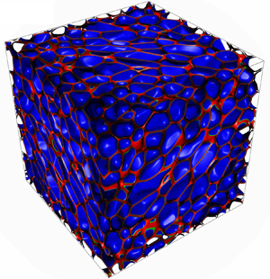
  $t=t_F$, for different volume fractions. Semi-dilute emulsions present a high number of small spherical droplets, whereas concentrated emulsions are constituted of a smaller number of non-spherical larger droplets. We report in table 1 the mean and root mean square (r.m.s.) values of some relevant observables (averaged in space and in time over the stirred phase, $t\in [t_0, t_F]$, and over the ageing phase, $t\in [7 \times 10^6, 9 \times 10^6]$, respectively), for the various volume fractions considered. One can immediately notice that, on increasing the volume fraction, accelerations and velocities r.m.s. decrease, implying a higher effective viscosity, while at the same time, the trend of the r.m.s. droplet diameter, $d_{rms}$, shows an increase in polydispersity.

Figure 1. Number density of droplets,  $N_D/L^3$, as a function of time for a set of four simulations, labelled with the corresponding target (steady state) volume fractions ( $\phi$) of the dispersed phase (see table 1 for further details). The solid lines (colour coded for the droplet number density) indicate the time evolution of the volume fraction during emulsification. The vertical dashed line highlights the starting time of tracking, $t_0 = 1.25 \times 10^6$. All simulations are stirred with the same forcing amplitude parameter ( $A=4.85\times 10^{-7}$, see (2.6)), except for the case indicated with hollow circles ( $A=4.05 \times 10^{-7}$, run labelled as $\phi _6$ in table 1). The relaxation phase $t \in [t_F, t_A^{(i)}]$ is omitted for the sake of clarity of visualisation.
Table 1. Relevant averaged quantities from the simulations at the different volume fractions  $\phi$. The overline, $\overline {()}$, indicates time average, the brackets, $\langle () \rangle$, indicate an average over time and over the ensemble of droplets. The superscripts $(s,a)$ indicate that the averages have been taken over the statistically steady stirring regime ( $t \in [t_0, t_F]$) and over the ageing regime ( $t\in [7\times 10^6, 9\times 10^6]$), respectively. The various columns contain: $t_{inj}$, injection endtime; $\overline {N_D}^{(s)}$, mean droplet number (stirring); $U^{(s)}_{rms}$, r.m.s. droplet velocity (stirring); $a^{(s)}_{rms}$, r.m.s. droplet acceleration (stirring); $T_L^{(s)}=L/U^{(s)}_{rms}$, large eddy turnover time (stirring); $\langle d \rangle$, mean droplet diameter; $d_{rms}$, standard deviation of the droplet diameter; $t_G$, mean (dimensionless) droplet life time; $U^{(a)}_{rms}$, r.m.s. droplet velocity (ageing); $a^{(a)}_{rms}$, r.m.s. droplet acceleration (ageing); $T_L^{(a)}=L/U^{(a)}_{rms}$, large eddy turnover time (ageing). Numerical values of the simulations parameters are: kinematic viscosity, $\nu =1/6$; total fluid density, $\rho _f = 1.36$; surface tension, $\varGamma =0.0238$ (correspondingly, the capillary number, based on the r.m.s. velocity, $Ca = \eta U_{rms}/\varGamma$, ranges between $Ca=0.16$ and $Ca=0.27$, for the highest and lowest volume fractions, respectively); forcing amplitude, $A=4.85\times 10^{-7}$ (except for the run $\phi _6$ for which $A=4.05 \times 10^{-7}$); simulation box side, $L=512$.


Figure 2. Snapshots from the stirred regime showing the morphology of the emulsions. On increasing the volume fraction,  $\phi$, a lower number of larger droplets are observed. Volume fractions below $\phi _c = 64\,\%$ (a value compatible with the random close packing of spheres in three dimensions) are characterised by spherical droplets, whereas higher fractions ( $\phi > \phi _c$) clearly show highly deformed droplets. More quantitative details can be found in table 1. Panels show (a) $\phi =38\,\%$, (b) $\phi =64\,\%$, (c) $\phi =70\,\%$, (d) $\phi =77\,\%$.
Figure 3 shows the mean rates of breakup ( $\bar {\beta }$) and coalescence ( $\bar {\kappa }$), i.e. the number of events per unit time, averaged over the stirred regime as a function of the volume fraction $\phi$ (in the inset we report $\beta (t)$ and $\kappa (t)$ as a function of time for $\phi = 70\,\%, 77\,\%$). In the steady state, the system is in a dynamical equilibrium with $N_D(t)$ essentially constant (see figure 1), therefore the breakup and coalescence rates approximately balance each other, $\beta (t) \approx \kappa (t)$; moreover, both mean rates are extremely low ( ${\sim }10^{-3}$) for $\phi < \phi _c = 64\,\%$, i.e. below jamming (in this regime, in particular for the lowest volume fraction considered, we detect very few events, which makes the statistical error relatively high and justifies the discrepancy between $\bar {\beta }$ and $\bar {\kappa }$), whereas they increase steeply with $\phi$ for $\phi >\phi _c$. Interestingly, $\phi _c$ is in the expected range of volume fractions for random close packing of spheres in three dimensions (Torquato & Stillinger Reference Torquato and Stillinger2010). The growth of $\bar {\beta }$ and $\bar {\kappa }$ above $\phi _c$ is particularly steep, suggesting a divergent behaviour as the volume fraction approaches a ‘critical’ value which can be arguably identified with the occurrence of the catastrophic phase inversion, $\phi _{cpi}$. A further hint to a critical phenomenon is given in the insets where $\bar {\beta }$, $\bar {\kappa }$ (bottom) and the mean droplet diameter $\langle d \rangle$ (top) are shown in doubly logarithmic plots vs $\phi _{cpi}-\phi$, highlighting the power-law character of the divergence.

Figure 3. (Main panel). Mean breakup ( $\bar {\beta }$) and coalescence ( $\bar {\kappa }$) rates (averaged over stirred regime) as a function of the volume fraction concentration $\phi$. The rates equal each other, consistently with the dynamical equilibrium observed at steady state; both rates are very low ( ${\sim }10^{-3}$) and basically insensitive to the volume fraction below jamming ( $\phi _c \approx 64\,\%$) and above it they increase steeply with $\phi$. The solid line represents the function $g(\phi ) = {C}/{(\phi _{cpi} - \phi )^q}$, which is telling us that the mean breakup and coalescence rates tend to diverge as the volume fraction approaches a critical value $\phi _{cpi}$, identifiable with that of catastrophic phase inversion (whence the subscript); fitting values of the parameters are $\phi _{cpi}=90.5\,\%$, $q=4.5$ and $C \approx 3.6 \times 10^4$. (Bottom inset) Log–log plot of the mean breakup and coalescence rates as function of the distance from $\phi _{cpi}$; the solid line is the function $g(\phi )$. (Top inset) Mean droplet diameter as a function of $\phi _{cpi}-\phi$; the solid line is a power-law fit with exponent $-0.52$.
The number of breakup and coalescence events depends, of course, on the intensity of the hydrodynamic stresses involved. To see how these quantities can give a flavour of the stability of the emulsion to the applied forcing, let us introduce an average droplet life time,  $t_G = {\overline {N_D}U_{rms}}/{\bar {\beta }L}$, non-dimensionalised by the large eddy turnover time; from table 1, we see that, below jamming ( $\phi \leq \phi _c$) $t_G \gg 1$, i.e. the droplets, on average, tend to preserve their integrity during the whole simulation, whereas, in the densely packed systems ( $\phi > \phi _c$), $t_G$ abruptly drops (down to $t_G \approx 0.1$ for the largest volume fraction, $\phi =77\,\%$).
3.1. Velocity and acceleration statistics: stirred regime
In figure 4 we report the p.d.f.s of the droplet velocities for volume fractions  $\phi =38\,\%$, $\phi =64\,\%$ and $\phi =77\,\%$. In both cases the p.d.f.s show a bell shape, but in a range of intermediate values of velocities $|v|$ they develop regions with non-monotonic curvature, which are more pronounced in the concentrated case. We ascribe such a peculiar shape to the droplet–droplet interactions (collisions and/or elastoplastic deformations). The characteristic velocity $v_c$ can be then estimated from the balance of the elastic force and the Stokesian drag for a spherical droplet of diameter $d$,
$d$,  $F_S = 3{\rm \pi} \eta d v_c$. The elastic force acting on droplets squeezed against each other is due to the disjoining pressure $\varPi$ stabilising the inter-droplet thin film; at mechanical equilibrium the disjoining pressure equals the capillary pressure at the curved droplet interface (Derjaguin & Churaev Reference Derjaguin and Churaev1978), therefore, the force can be estimated as the Laplace pressure times the cross-sectional area, $F_{el} \sim ({2\varGamma }/{d}){\rm \pi} ({d}/{2})^2$, where $\varGamma$ is the surface tension. Letting $F_{el} \sim F_S$ gives $v_c \sim {\varGamma }/{6\eta } = 0.0175$; from figure 4 we see that, indeed, the inflections are located around $v\sim \pm v_c$. To test our conjecture further, we have run a simulation setting the competing lattice interactions responsible for the emergence of the disjoining pressure to zero ( $G_{{OO},1}=G_{{WW},1}=G_{{OO},2}=G_{{WW},2}=0$ in (2.5)), thus, effectively, we enforce $\varPi =0$. The resulting velocity p.d.f. is reported in figure 4, where we observe that, in fact, the inflectional regions disappear.

Figure 4. Probability density functions (p.d.f.s) of the droplet velocities (in units of their respective r.m.s. values), for  $\phi =38\,\%$, $\phi =64\,\%$ and $\phi =77\,\%$, computed over the forced steady state. In all cases the curves show two marked inflection points, around $v \approx \pm v_c = 0.0175$ (indicated with vertical dashed lines for $\phi =38\,\%$, thin line, and $\phi =77\,\%$, thick line), which are, instead, suppressed when the disjoining pressure is deactivated, $\varPi =0$ (solid line).
The p.d.f. of droplet accelerations, reported in figure 5, is Gaussian in the semi-dilute emulsion ( $\phi = 38\,\%$) but, as the volume fraction is increased above $\phi _c = 64\,\%$, the p.d.f.s tend to develop fat (non-Gaussian) tails. A working fitting function is a stretched exponential of the type
 \begin{equation} P(\tilde{a})=C \exp\left(-\frac{\tilde{a}^{2}}{\left(1+\left(\dfrac{\beta |\tilde{a}|}{\sigma}\right)^{\gamma}\right)\sigma^{2}}\right)\!, \end{equation}
where  $\tilde {a}=a/a_{rms}$. The non-Gaussianity here, unlike turbulence, cannot be grounded on the complexity of the velocity field and of the associated multifractal distribution of the turbulent energy dissipation (Biferale et al. Reference Biferale, Boffetta, Celani, Devenish, Lanotte and Toschi2004). We are not facing, in fact, a fully developed turbulent flow and, moreover, the non-Gaussian signatures become evident on increasing the volume fraction above the jamming point $\phi _c$, where the effective viscosity is higher (and, hence, the effective Reynolds number is lower). The origin of the non-Gaussianity is to be sought in the complex elastoplastic dynamics of the system, which is driven by long-range correlated irreversible stress relaxation events. Remarkably, in concentrated emulsions, it has been shown that the spatial distribution of stress drops in the system displays a multifractal character (Kumar et al. Reference Kumar, Korkolis, Benzi, Denisov, Niemeijer, Schall, Toschi and Trampert2020), which might be responsible for the statistical properties of the acceleration at high volume fraction, in formal analogy with the phenomenology of turbulence. The curves corresponding to (3.1) are reported in figure 5, for various values of the parameter $\gamma$, which gauges the deviations from the Gaussian form, and fixed $\beta =0.35$ (obtained from best fitting) and $\sigma =1$, the standard deviation of the Gaussian limit, such that, for $\gamma = 0$, the p.d.f. reduces to the normal distribution $\propto \textrm {e}^{-x^2/2}$. This is, indeed, the case for the lowest volume fraction, $\phi = 38\,\%$; the non-Gaussianity parameter $\gamma$ then increases monotonically with $\phi$ up to $\gamma = 1.6$ for $\phi = 77\,\%$.

Figure 5. The p.d.f.s of the droplet accelerations, for  $\phi =38\,\%, 64\,\%, 77\,\%$, computed over the statistically steady forced state. The p.d.f.s are normalised to have unitary area. The values of $a_{rms}$ are given in table 1. The solid lines are fits from (3.1) with $\sigma =1$ and $\beta =0.35$, whereby the non-Gaussianity parameter $\gamma$ takes the values $\gamma =0$ (corresponding to the Gaussian distribution) for $\phi =38\,\%$, $\gamma =1.32$ for $\phi =64\,\%$ and $\gamma =1.6$ for $\phi =77\,\%$.
3.2. Dispersion: stirred regime
We focus now on the spatial dispersion of both single droplets as well as of droplet pairs. The single-droplet (or absolute) dispersion is defined in terms of the statistics of displacements,  $\Delta \boldsymbol {X} = \boldsymbol {X}(t_0 + T) - \boldsymbol {X}(t_0)$, where $\boldsymbol {X}(t)$ is the position of the droplet centre of mass at time $t$ (
$t$ ( $t_0=1.25 \times 10^6$, let us recall, is the starting time of tracking). In figure 6 we show the mean square displacement (MSD), $\langle \Delta X^2 \rangle$, for volume fractions $\phi =38\,\%, 64\,\%$ and $77\,\%$. Values are reported in logarithmic scale, with the time normalised (hereafter) by a characteristic large-scale time defined as $t_L = \sqrt {\rho _f L/A} \approx 38\,000$ (which is independent of the volume fraction), where $A$ is the amplitude of the applied forcing (so $A/\rho _f$ is an acceleration). In the diluted case, the MSD (figure 6) shows a cross-over at around $T \sim 5 t_L$ between an initial ballistic motion, $\langle \Delta X^2 \rangle \sim T^2$, and a diffusive behaviour at later times, $\langle \Delta X^2 \rangle \sim T$. This is consistent with the typical Lagrangian dynamics of particles advected by chaotic and turbulent flows (Falkovich, Gawedzki & Vergassola Reference Falkovich, Gawedzki and Vergassola2001); for intermediate times, however, we observe a transitional region, in correspondence, approximately, with the cross-over, where the curve presents an inflection point with a locally super-ballistic slope. This is an interestingly non-trivial behaviour that certainly deserves further investigation. On increasing the volume fraction above $\phi _c$ the long-time growth seems to become steeper, although no clear conclusion can be reached due to the extremely small range available in the numerical simulation. A deeper insight into the small-scale dynamics can be grasped by looking at the pair dispersion, namely the statistics of separations
 \begin{equation} \boldsymbol{R}_{ij}(t) = \boldsymbol{X}_i(t) - \boldsymbol{X}_j(t), \end{equation}
at time  $t$ for all pairs of droplets $i,j$ that are nearest neighbours (i.e. such that their corresponding cells in a Voronoi tessellation of the centre of mass distribution are in contact) at $t=t_0$. The observable in (3.2) is, in fact, insensitive to contamination from mean homogeneous large-scale flows, if present. In figure 7 we report the mean square value $R^2(t) \equiv \langle |\boldsymbol {R}_{ij}|^2 \rangle _{\{ij\}}$ (where the average is over the initially neighbouring pairs) as a function of time, for $\phi = 38\,\%, 64\,\%$ and $77\,\%$. Analogously to the MSD, $R^2(t)$ grows in time and, after an initial ballistic transient, it follows a diffusive-like behaviour. Again, for $\phi > \phi _c$, one may argue about a superdiffusive behaviour.

Figure 6. The MSD,  $\langle \Delta X^2 \rangle$, for $\phi =38\,\%, 64\,\%$ and $77\,\%$, in the forced regime. The MSD goes initially as $T^2$, indicating a ballistic dynamics, followed by a diffusive growth, $T^{1/2}$, for $\phi < \phi _c$, whereas in the densely packed system ( $\phi =77\,\%$), there is a superdiffusive behaviour $T^{\alpha }$, with $\alpha = 1.15$.

Figure 7. Mean square droplet pair separation  $R^2(t) \equiv \langle |\boldsymbol {R}|^2 \rangle$ as a function of time for volume fractions $\phi = 38\,\%, 64\,\%, 77\,\%$. The power laws are reported as solid lines, evidencing a slight deviation from the diffusive regime for the most concentrated case.
3.3. Velocity and acceleration statistics: ageing regime
When the large-scale forcing is switched off, in diluted conditions (below the close packing volume fraction), the system relaxes via a long transient, where the kinetic energy decays to zero. Instead, at high volume fraction (in the jammed phase), the emulsion is never completely at rest, due to diffusion and droplet elasticity favouring the occurrence of plastic events, namely, the local topological rearrangement of a few droplets (i.e. during the ‘ageing’ of the material). Therefore, we consider here only the latter situation and focus on the case  $\phi = 77\,\%$; hereafter, we present data obtained with forcing amplitude $A=4.05 \times 10^{-7}$ (see the $\phi _6$ row in table 1), which yielded a larger number of droplets ( ${\sim }10^3$) in the steady state, which improved the statistics. The p.d.f. of the droplet velocities is reported in figure 8. Since there is no mean flow, the p.d.f. is an even function of its argument. We show, therefore, the distribution of the absolute values in logarithmic scale, in order to highlight the power-law behaviour $v^{-3}$. Interestingly, the p.d.f. of acceleration also develops a power-law tail $P(a) \sim a^{-3}$ (the p.d.f.s for velocity and acceleration do, in fact, overlap, upon rescaling by the respective standard deviations, see figure 8), reflecting the fact that, when stirring is switched off, the high effective viscosity overdamps the dynamics, thus enslaving the acceleration to the velocity (by Stokesian drag), $a \sim u/\tau _s$ (assuming the Stokes time is equal for all droplets, which is reasonable given the very low spread of size distribution in the ageing regime Girotto et al. Reference Girotto, Benzi, Di Staso, Scagliarini, Schifano and Toschi2022).

Figure 8. The p.d.f.s of the absolute values of droplet velocities and accelerations, rescaled by their own r.m.s. values (given in table 1), in the ageing regime. Both p.d.f.s show a power-law,  $P(\zeta ) \sim \zeta ^{-3}$, decay.
3.4. Dispersion: ageing regime
In the ageing regime at the largest volume fraction,  $\phi =77\,\%$, the MSD goes as $\langle \Delta X^2 \rangle \sim T^2$ for short times, signalling a ballistic regime, followed by a super-diffusive regime $\langle \Delta X^2 \rangle \sim T^{3/2}$ (see inset of figure 9). The short-time ballistic regime is consistent with a theoretical prediction based on the superposition of randomly distributed elastic dipoles (following structural micro-collapses) (Bouchaud & Pitard Reference Bouchaud and Pitard2001) and with results from experiments with colloidal gels (Cipelletti et al. Reference Cipelletti, Manley, Ball and Weitz2000) and foams (Giavazzi et al. Reference Giavazzi, Trappe and Cerbino2021). The scaling $\langle \Delta X^2 \rangle \sim T^{3/2}$ is, instead, slightly steeper than the experimentally measured ${\sim }T^{1.2}$ (Giavazzi et al. Reference Giavazzi, Trappe and Cerbino2021).

Figure 9. Absolute dispersion of droplets in the ageing regime at  $\phi =77\,\%$. (Main panel) The p.d.f.s of droplet displacements (van Hove functions) at two time increments $T$, in the ageing regime; for the time increment in the ballistic regime the p.d.f. shows, as expected, a $\Delta X^{-3}$ decay, consistent with the velocity p.d.f., figure 8. (Inset) Mean square displacement, $\langle \Delta X^2 \rangle$, vs time increment; the solid lines highlight the ballistic and superdiffusive behaviours.
The ballistic regime  $\langle \Delta X^2 \rangle \sim T^2$ entails a power-law tail of the p.d.f. of separations for short times, $P(\Delta X) \sim \Delta X^{-3}$, corresponding to the self-part of the van Hove distribution (Hansen & McDonald Reference Hansen and McDonald1986), as reported in figure 9 (Cipelletti et al. Reference Cipelletti, Ramos, Manley, Pitard, Weitz, Pashkovski and Johansson2003; Giavazzi et al. Reference Giavazzi, Trappe and Cerbino2021). This observation finds correspondence, as one could expect, in the p.d.f. of the droplet velocities, shown in figure 8.
The study of pair dispersion, reported in figure 10, evidences, for the mean square pair separation (in the inset), a ballistic regime,  $\langle R^2 \rangle \sim t^2$, followed by a superdiffusive behaviour, $\langle R^2 \rangle \sim t^{4/3}$. The persistence of ballistic motion is expected to match the decorrelation of trajectories following a plastic event, therefore the cross-over time, $t_c$, can be approximately estimated as the time taken by a droplet to travel the typical size of a rearrangement, $\xi \approx 2 d$ (which is an intrinsic scale for correlation lengths in soft glassy materials Goyon et al. Reference Goyon, Colin, Ovarlez, Ajdari and Bocquet2008; Dollet et al. Reference Dollet, Scagliarini and Sbragaglia2015); since the characteristic velocity is $v_c \sim {\varGamma }/{6\eta }$ (see figure 4 and discussion thereof), we get $t_c \sim {12 d \eta }/{\varGamma } \approx 7 \times 10^3$, indicated in the inset of figure 10 with a dashed line.

Figure 10. (Main panel) The p.d.f.s of the pair separations,  $P(R,t)$ at two instants of time in the super-diffusive regime, $t_{1,2}>t_c$; the solid lines are the theoretical prediction, (3.5), with parameters $\mathcal {A}=1.7$, $c = 6 \times 10^{-4} < d >^{3/2} t_c^{-1}$. (Inset) Mean square separation as a function of time: a ballistic regime, $\langle R^2 \rangle \sim t^2$, is followed by a super-diffusive one, $\langle R^2 \rangle \sim t^{4/3}$, the cross-over between the two regimes occurring around $t \approx t_c = 12 d \eta /\gamma$, indicated with the dashed line.
By analogy with Richardson's description of turbulent diffusion (Richardson Reference Richardson1926; Falkovich et al. Reference Falkovich, Gawedzki and Vergassola2001; Boffetta & Sokolov Reference Boffetta and Sokolov2002), we propose a phenomenological approach to derive the full pair separation p.d.f. in the superdiffusive regime. We assume that the p.d.f. evolves according to a generalised diffusion equation, with a scale-dependent effective diffusivity,  $D_{eff}$ which, dimensionally, should be proportional to ${\textrm {d} \langle R^2 \rangle }/{\textrm {d}t}$. Since $\langle R^2 \rangle \sim t^{4/3}$ (and, consequently, $t \sim R^{3/2}$), we have
 \begin{equation} D_{eff} \propto \frac{{\rm d} \langle R^2 \rangle}{{\rm d}t} \sim t^{1/3} \quad \Rightarrow \quad D_{eff} \propto R^{1/2} \equiv c R^{1/2}. \end{equation}
The diffusion equation thus reads
 \begin{equation} \partial_t P(R,t) = \partial_{R} \left(cR^{1/2} \partial_{R} P(R,t)\right)\!, \end{equation}
that admits as solution (with the condition of unit area at all times) the following non-Gaussian distribution:
 \begin{equation} P(R,t) = \mathcal{A}\frac{2R^2}{27c^2 t^2}\exp\left(-\frac{4 R^{3/2}}{9ct}\right)\!. \end{equation}
The p.d.f.s of pair separations measured at two instants of time in the superdiffusive regime,  $t_1 \approx 150 t_c$ and $t_2 \approx 300 t_c$, are shown in figure 10 together with the prediction of (3.5), with fitting parameter $c = 6\times10^{-4} \langle d\rangle^{3/2} t_c^{-1}$, plotted as solid lines. The agreement obtained between theory and numerics is quite remarkable.
4. Conclusions
In this paper, using 3-D numerical simulations, we discussed the complex statistical and dynamical properties of concentrated emulsions. The simulations were carried out using a recently developed procedure for in silico emulsification (Girotto et al. Reference Girotto, Benzi, Di Staso, Scagliarini, Schifano and Toschi2022) which is based on the modelling of stabilised binary immiscible liquid mixtures with high volume fractions of the dispersed phase. We also developed a novel tracking algorithm that allowed us to study the emulsion physics at the droplet-resolved scale from a Lagrangian viewpoint, across various concentrations, from the semi-dilute to the jammed regimes.
Using the same large-scale forcing, we studied the mean rates of droplet breakup  $\bar {\beta }$ and coalescence $\bar {\kappa }$, the droplet velocity, acceleration and dispersions. We have shown that $\bar {\beta }$, $\bar {\kappa }$ and the average droplet diameter $\langle d \rangle$ show a divergent-like behaviour for $\phi$ close to the catastrophic phase inversion $\phi _{cpi}$.
Also, we highlighted how the elastic properties and the plastic microdynamics of densely packed ensembles of droplets in close contact are responsible of the non-Gaussian character of the droplet acceleration and, more moderately, of the velocity statistics.
We further investigated the single-droplet diffusion in terms of both the MSD and the self-part of the van Hove distribution functions. In particular. for a rather large value of  $\phi$, we stopped the large-scale forcing and we studied the so-called aging regime. We observe a well-defined cross-over in time from ballistic to super-diffusive behaviour, in agreement with previous theoretical and experimental results. Further investigations will focus on the dispersion properties on larger systems and for longer observation times, as well as on the relation of the Lagrangian properties of the droplets to the stress distribution throughout the system. In perspective, we foresee extending of the reach of the present work to extreme conditions of volume fractions and forcing amplitudes, whereby the emulsion tends to lose stability and to undergo a catastrophic phase inversion. In this limit, too, the Lagrangian approach is of invaluable utility. Overall, our approach suggested a bridge between classical tools for Lagrangian high Reynolds number flows and complex fluid rheology, which paves the way to the inspection of unexplored aspects of the physics of soft materials.
Acknowledgements
We are thankful to C. Sun and L. Yi for useful discussions and P. Perlekar for a fruitful interaction at the initial stage of the work.
Funding
Numerical simulations were performed thanks to granted PRACE projects (ID: 2018184340 and 2019204899) along with CINECA and BSC for access to their HPC systems. This work was partially sponsored by NWO domain Science for the use of supercomputer facilities.
Declaration of interests
The authors report no conflict of interest.


 Open access