


1. Introduction
Understanding and predicting extreme events remains an open problem in turbulence research with important theoretical and practical implications. Particularly now, in the context of climate change (Rahmstorf & Coumou Reference Rahmstorf and Coumou2011; Stott Reference Stott2016), interest has emerged to develop models and indicators which afford early warnings of extreme events (Travis Reference Travis2010; Alfieri et al. Reference Alfieri, Salamon, Pappenberger, Wetterhall and Thielen2012; Vitart & Robertson Reference Vitart and Robertson2018). These models are usually constructed using variational principles (Farazmand & Sapsis Reference Farazmand and Sapsis2017; Blonigan, Farazmand & Sapsis Reference Blonigan, Farazmand and Sapsis2019), reduced-order modelling (Chen & Majda Reference Chen and Majda2020) or machine learning (Lellep et al. Reference Lellep, Prexl, Linkmann and Eckhardt2020; Qi & Majda Reference Qi and Majda2020; Fernex, Noack & Semaan Reference Fernex, Noack and Semaan2021; Lellep et al. Reference Lellep, Prexl, Eckhardt and Linkmann2022), and their performance is partly limited by their ability to parse complex dynamics (Kaszás & Haller Reference Kaszás and Haller2020). A more fundamental limitation stems from the uncertainty in the initial conditions, which is amplified in time by the chaotic dynamics, and imposes a maximum or ideal temporal limit beyond which predictions become impossible (Lorenz Reference Lorenz1963).
Predictability is characterised in general by the Lyapunov exponents (Boffetta et al. Reference Boffetta, Cencini, Falcioni and Vulpiani2002), which measure the rate of separation of trajectories starting from neighbouring initial conditions (Lorenz Reference Lorenz1965; Aurell et al. Reference Aurell, Boffetta, Crisanti, Paladin and Vulpiani1997; Ziehmann, Smith & Kurths Reference Ziehmann, Smith and Kurths2000). In particular, the sum of the positive Lyapunov exponents, the Kolmogorov–Sinai entropy, quantifies the rate at which different possible future states emerge from the present state of the system (Boffetta et al. Reference Boffetta, Cencini, Falcioni and Vulpiani2002). However, the Lyapunov exponents are very sensitive to small-scale dynamics (Aurell et al. Reference Aurell, Boffetta, Crisanti, Paladin and Vulpiani1997; Budanur & Kantz Reference Budanur and Kantz2022) and are only useful to characterise short-time predictability (Palmer Reference Palmer1993). Moreover, their relationship to certain features of the flow, such as extreme events, is not straightforward. Specifically, the predictability of extreme events is not concerned with the number of different possible future states, but with the fraction of them that will be extreme. This information is given by the evolution of probability distributions in the phase space of the system, which is difficult to model due to the high dimension of the chaotic attractor underlying turbulent flows (Epstein Reference Epstein1969; Palmer Reference Palmer2000). In general, it is unclear how far in advance extreme events can be predicted and by how much predictive models can be improved.
In this paper, we investigate the ideal predictability limit of extreme events in a two-dimensional turbulent flow driven by a Kolmogorov (sinusoidal) forcing. We consider the Navier–Stokes equations as a perfect forecasting model, and reproduce the uncertainty of the initial conditions using small random perturbations, a technique known as Monte Carlo forecasting (Epstein Reference Epstein1969). We produce massive ensembles of perturbations to accurately describe the temporal evolution of probability distributions and quantify predictability as the information gained by forecasting under these ideal conditions. We show that the predictability of extreme events fluctuates strongly across the attractor and that it depends on the state from which the extreme event emerges.
2. Forecasting the Kolmogorov flow with massive ensembles
The two-dimensional Kolmogorov flow is spatially extended, deterministic and chaotic, and features some of the complex dynamics of turbulence, in particular, the strong bursting (Kim, Kline & Reynolds Reference Kim, Kline and Reynolds1971; Encinar & Jiménez Reference Encinar and Jiménez2020) and extreme episodes of the dissipation (Hack & Schmidt Reference Hack and Schmidt2021). It has been widely used as a testbed for reduced-order modelling (Fernex et al. Reference Fernex, Noack and Semaan2021), to describe the geometry of the phase space with simple invariant solutions of the equations (Chandler & Kerswell Reference Chandler and Kerswell2013; Lucas & Kerswell Reference Lucas and Kerswell2015; Suri et al. Reference Suri, Tithof, Grigoriev and Schatz2017; Page, Brenner & Kerswell Reference Page, Brenner and Kerswell2021) and for the prediction of extreme dissipation events (Farazmand & Sapsis Reference Farazmand and Sapsis2019; Sapsis Reference Sapsis2021). This flow is governed by the two-dimensional Navier–Stokes equations (NSEs) in a doubly periodic square domain of area  $L^2=(2{\rm \pi} )^2$,
 \begin{equation} \partial_t \omega + \boldsymbol u \boldsymbol{\cdot}\boldsymbol{\nabla} \omega=\nu\nabla^2 \omega + f, \end{equation}
where  $\nu$ is the kinematic viscosity, $\omega =(\boldsymbol {\nabla }\times \boldsymbol u)_z$ is the vorticity in $z$ (the direction normal to the $x$–
$x$– $y$ plane) and $\boldsymbol u$ is the velocity vector, which satisfies the incompressibility condition, $\boldsymbol {\nabla }\boldsymbol{\cdot}\boldsymbol u=0$, and is obtained from $\omega$ using a stream function. The forcing of the flow acts on the velocity field as $\boldsymbol {f}_u=\{\,f_0(L/2{\rm \pi} )\cos (2{\rm \pi} n_f y/L),0\}$, where $f_0$ is the forcing magnitude and $n_f=4$ its wavenumber. In the vorticity equation (2.1), the forcing reads
 \begin{equation} f=f_0 n_f \sin(2{\rm \pi} n_f y/L). \end{equation}
The flow is characterised by a Reynolds number,
 \begin{equation} Re=f_0^{1/2}(L/2{\rm \pi})^{2}/\nu, \end{equation}
as defined by Chandler & Kerswell (Reference Chandler and Kerswell2013) and Farazmand & Sapsis (Reference Farazmand and Sapsis2017). In this work, we set  $Re=100$. The vorticity is normalised with $f_0^{1/2}$ and the time with the Lyapunov time, $T_\lambda =\lambda ^{-1}$, where $\lambda$ is the leading Lyapunov exponent, which is calculated following a rescaling method over a long trajectory (Wolf et al. Reference Wolf, Swift, Swinney and Vastano1985). For comparison, the time scale of the forcing is $T_f=1/{f_0}^{1/2}=0.28T_\lambda$ and the eddy turnover time is $T_{{eto}}={(\nu /\bar {\varepsilon })}^{1/2}=1.92T_\lambda$, where the overline denotes temporal average and $\varepsilon$ is the spatially averaged energy dissipation. Another important time scale is the delay between energy injection due to the forcing and the dissipation, $T_I=0.66T_\lambda$, which we obtained from their temporal cross-correlation.
The flow is integrated using a pseudo-spectral method with a Fourier basis of  $N/2$ modes in each direction, where $N=128$ is the number of points in physical space. This is similar to the resolution used by Lucas & Kerswell (Reference Lucas and Kerswell2015). The nonlinear terms are fully dealiased using a $2/3$ rule, and a third-order low-storage Runge–Kutta method is used for time marching. The simulations are carried out using a GPU code based on the spectral solver described by Cardesa, Vela-Martín & Jiménez (Reference Cardesa, Vela-Martín and Jiménez2017), which enables a massive exploration of phase space at a moderate cost.
We aim to determine the predictability of the instantaneous space-averaged enstrophy,
 \begin{equation} \varOmega=\langle\omega^2\rangle, \end{equation}
where the brackets denote the spatial average over the computational domain. Note that  $\varOmega =\varepsilon /\nu$, so we interchangeably use dissipation and enstrophy throughout. We use the Navier–Stokes equations as a perfect forecasting model so that uncertainty is only due to the initial conditions. First, we sample the chaotic attractor with a set of $N_{i}=8192$ independent states $\omega _i$, hereafter termed base flows. These base flows represent possible states of the system from which an extreme enstrophy event may eventually arise, as exemplified for two cases in figure 1. This figure shows two events of magnitude $\varOmega \approx 9$, which correspond to the upper $1\,\%$ of the enstrophy probability distribution in the attractor. The average waiting time between events of this magnitude is more than $90T_\lambda$. Despite the marked differences between the initial circulation patterns in the first and second rows, at peak enstrophy, the flow patterns are remarkably similar in topology and intensity.

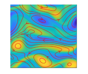
Figure 1. Visualisations of two independent realisations of the Kolmogorov flow (a,b) before and during an enstrophy burst of magnitude  $\varOmega >9$; the corresponding time series of $\varOmega (t)$ are shown in figure 2(a,d). Time goes from left to right, $t=0$, $1.5$, $3$,
$3$,  $4.4$ and $t_{e}$, where $t_e=5.9$ and $t_e=5.6$ is the time of the extreme event in the runs in panels (a) and (b), respectively. The colour map shows the vorticity, $\omega$, from $-$8 (dark blue) to $8$ (yellow), and the red lines are streamlines of the instantaneous velocity field. Initially, the flow is organised in large-scale swirls, sometimes with the presence of vertical velocity jets (bottom-left panel), whereas during the burst, the vorticity is predominantly aligned horizontally, parallel to the forcing driving the flow.

Figure 2. (a) Temporal evolution of the enstrophy  $\varOmega _i(t)$ (red solid line) in the base trajectory visualised in figure 1(a). The shaded area spans from the first to the last decile of $\varOmega _{i,p}(t)$ in the corresponding ensemble. The markers denote the instants in time shown in figure 1(a). (b) Forecast probability distribution $P_i(t)$ at the time instants indicated in the legend and marked with points in figure 1(a). The climatological distribution $Q$ is shown as a dashed line. (c) Temporal evolution of the Kullback–Leibler divergence, $D_i(t)$, for the base trajectory in figure 1(a). The points are as in figure 1(a). (d,e) As in panels (a–c), but for the predictable base trajectory in figure 1(b). In panel (f), the shaded are spans from the first to the last decile of the KLD in all the ensembles.
We assess the predictability of the  $N_{i}=8192$ base flows by performing a Monte Carlo ensemble forecast (Leith Reference Leith1974; Leutbecher & Palmer Reference Leutbecher and Palmer2008), in which the uncertainty in the initial state of the system is modelled by small random perturbations. Around each base flow $\omega _i(\boldsymbol x,t_0)$, we produce $N_{p}=8192$ perturbed flows,
 \begin{equation} \omega_{i,p}(\boldsymbol x,t_0)=\omega_i(\boldsymbol x,t_0) + \phi(\boldsymbol x), \end{equation}
with a different realisation of the random perturbation field,  $\phi (\boldsymbol x)$, which is Gaussian noise with a white spectrum and variance $\sigma ^2=0.01f_0$. In the perturbed fields, $\omega _{i,p}$, the first subscript refers to the base flow and the second subscript to the perturbation. The small magnitude of the initial perturbations ensures that they first evolve according to the linearised dynamics and that they have time to align with the most unstable local directions before triggering nonlinear effects. Thus, the results are independent of the structure of the random perturbation. We have verified this by perturbing the velocity field (instead of the vorticity field) with the same magnitude of the random perturbations. The corresponding analysis is described in Appendix A. Predictability depends naturally on the initial uncertainty, i.e. on the variance of the noise, $\sigma ^2$, but given its magnitude, this dependence is weak and only relevant for the initial stage of perturbation growth. This stage, which in our ensembles corresponds to a time of the order of $T_\lambda$, increases only logarithmically with decreasing $\sigma ^2$ due to the exponential growth of perturbations with time (see Appendix A).
In summary, we produced  $N_i=8192$ ensembles with $N_{p}=8192$ members, which were integrated in time, together with their base states, for $20$ Lyapunov times. To study the predictability of the enstrophy, we stored its temporal evolution, $\varOmega _{i,p}(t)$, in the $N_{i}N_{p}=2^{26}= 67\,108\,864$ runs. The probability density function (p.d.f.) of $\varOmega _{i,p}(t)$ of each ensemble $i$, denoted by $P_i(t)$, fully describes the possible values of the enstrophy and their likelihood at a future time $t$. In the next section, we show how $P_i(t)$ can be used to unambiguously quantify the predictability of $\varOmega$ and, in particular, of its extreme events.
3. Quantifying the predictability of extreme events with information-theoretic measures
In figure 2(a), we show the temporal evolution of  $\varOmega _i(t)$ in the base flow displayed in figure 1(a), and the values of $\varOmega _{i,p}$ contained between the first and last deciles of $P_i(t)$, represented as a shaded area. Initially, the values of the dissipation in the ensemble remain close to the base flow. Subsequently, the range of possible values of $\varOmega _{i,p}$ starts increasing noticeably in a time of the order of the Lyapunov time, indicating that the ensemble is being spread across the attractor. In figure 2(b), we show snapshots of $P_i(t)$ at selected times. Initially, $P_i$ has a small spread, but this increases with time. At the time of the extreme event in the base trajectory, $t_e=5.9$, the forecast distribution $P_i(t)$ is very similar to the (stationary) probability distribution of $\varOmega$ in the attractor, $Q$, which is known as the climatological distribution (DelSole Reference DelSole2004). Hence, with the level of uncertainty in the initial conditions (set by $\phi (\boldsymbol x)$ in (2.5)), forecasts obtained by solving the NSE are hardly more accurate than the null forecast, i.e. with the assumption that the initial condition was taken randomly from anywhere in the attractor. This means that, given the initial uncertainty, this extreme event is fundamentally unpredictable regardless of the forecasting model in a time horizon of $6T_\lambda$.
Predictability may be quantified with information-theoretic measures of how different  $P_i(t)$ is from the climatological probability distribution (Kleeman & Majda Reference Kleeman and Majda2005; DelSole & Tippett Reference DelSole and Tippett2007). We use the Kullback–Leibler divergence (KLD)
 \begin{equation} D_i(P_i(t)\,|\,Q)=\sum \tilde{P}_i(t) \log \frac{\tilde{P}_i(t)}{\tilde{Q}}, \end{equation}
where the tilde indicates that the probability distributions have been discretised in  $40$ intervals of equal width in the range $[1.5,13.5]$, which contain all the samples in the database. The summation is taken over these probability intervals. We have checked that reducing the number of members in the ensemble by a half produces only small variations of $D_i$. The KLD is always positive unless $P_i(t)=Q$, when it is zero (MacKay Reference MacKay2003). The more that $P_i(t)$ differs from $Q$, the larger $D_i$ and the more informative the ensemble forecast. In other words, $D_i$ is a measure of the amount of information we gain by forecasting with massive ensembles of NSE simulations with respect to taking the climatological distribution as the forecasting model (null forecast).
The temporal evolution of  $D_i$ for the base trajectory in figure 1(a) is shown in figure 2(c). It fluctuates, as has been observed previously for other information-theoretic measures in low-dimensional systems (Latora & Baranger Reference Latora and Baranger1999), but decreases overall with time. At the time of the extreme event in the base trajectory, the KLD has decreased by more than one order of magnitude with respect to its initial value, signalling the lack of information in the forecast distribution and the unpredictability of the extreme event, given the initial uncertainty.
We now examine the predictability of the extreme event displayed in figure 1(b). As shown in figure 2(d), this extreme event occurs at  $t_e\approx 5.6$ and has a magnitude similar to the event examined above. The evolution of the probability distribution of the ensemble, $P_{i}(t)$, is shown in figure 2(e). For this base flow, the probability distribution at $t_e$ is highly skewed towards large values, indicating that this extreme event is largely predictable. In figure 2(f), we show the temporal evolution of $D_i$ for the predictable (blue) and unpredictable (red) extreme events. There is a difference of an order of magnitude between their $D_i$ at the time of the extreme event. This is particularly remarkable given that the temporal evolution of $\varOmega$, and the flow patterns near the maximum enstrophy, are qualitatively similar. In figure 2(f), we have also plotted the evolution of the average (solid black line) and the first and last deciles (shaded area) of $D_i$ in the $8192$ base flows. Again, there is a difference of more than one order of magnitude between the first and last deciles, indicating that the strong fluctuations of predictability between the two trajectories of figure 1 are a general, intrinsic feature of the system.
The strong fluctuations in predictability are confirmed using another indicator: the ratio of successful predictions (RSPs) (Farazmand & Sapsis Reference Farazmand and Sapsis2017). For each base trajectory  $i$, we define an extreme event happening at time $t_e$ as a local maximum of $\varOmega _i$ in which $\varOmega _i>\alpha$, where $\alpha$ is a threshold. Now, we consider each ensemble member $p$ as an individual forecast and tag this forecast as successful (true positive) if it gives $\varOmega _{i,p}>\alpha$ at the time of the extreme event in the base trajectory, $t_e$. However, we tag this forecast as unsuccessful (false negative) if it gives $\varOmega _{i,p}<\alpha$ at $t_e$. In each ensemble, we calculate the number of true positives, $N_{{true\ pos.}}$ and false negatives $N_{{false\ neg.}}$, and define the RSP as
 \begin{equation} {RSP}=\frac{N_{{true\ pos.}}}{N_{{true\ pos.}} + N_{{false\ neg.}}}, \end{equation}
which depends on the time of the extreme event in the base trajectory,  $t_e$, and on the threshold $\alpha$. Since the number of members in the ensemble is $N_p=N_{{true\ pos.}} + N_{{false\ neg.}}$, the RSP is defined as the probability that $\varOmega _{i,p}>\alpha$ at $t_e$. In brief, the RSP quantifies the probability of making a successful forecast considering the initial uncertainty and taking the base trajectory as the true trajectory. Here the idea of successful prediction is considered with respect to an ideal forecasting model, i.e. the NSE, which is free of model uncertainty.
In figure 3, we show the RSP averaged over temporal intervals of width  $T_\lambda$, centred at integer times, for different thresholds. The RSP decreases on average with time and with the intensity of the extreme event. The standard deviation of the RSP in the intervals, shown as bars in the figure, is of the order of the average, corroborating the fluctuations of predictability measured by the KLD. In particular, for the event in figure 1(b), the probability that $\varOmega _{p,i}>8.0$ at $t_e$ is close to $50\,\%$ ( $RSP=0.5$), indicating that this event is largely predictable. By contrast, for the unpredictable extreme event in figure 1(a), this probability is less than $3\,\%$ ( $RSP=0.03$).

Figure 3. Average RSP as a function of the time of extreme events,  $t_e$, for different thresholds: $\varOmega >8$ (black line); $\varOmega >9$ (blue line); $\varOmega >10$ (red line). The average is calculated in time intervals centred at multiples of $T_\lambda$ and width $T_\lambda$. The bars in the blue line correspond to the mean plus-minus the standard deviation of the RSP in each interval (except when it is negative). For ease of visualisation, bars are only plotted for $\varOmega >9$, but are comparable for the other two cases.
4. Large-scale circulation patterns set the predictability limit of extreme events
In the following, we perform a conditional statistical analysis to determine the differences between predictable and unpredictable extreme events. From the  $N_i=8192$ base flows, we select those that exhibit a local maximum of the enstrophy in the time interval $3< t_e<17$ in which $\varOmega _i(t_e)>8$, where $t_e$ is the time of the maximum. We find that a total of $1040$ trajectories satisfy these criteria. The average enstrophy of this group of base trajectories, centred about $t_e$, is shown as a black line in figure 4(a). It remains close to the average in the attractor (shown as a horizontal dotted line) up to approximately $t-t_e\sim -3$, when it shoots up monotonically towards the extreme event.

Figure 4. (a) Conditional average dissipation. The black line shows the average of  $\varOmega _i$ over all base trajectories featuring an extreme event (with $\varOmega _i(t_e)>8$, for $3< t_e<17$). The red and blue lines show the average conditional to low and high predictability, respectively. The corresponding trajectories have a $D_i(t)$ below and above the first and last deciles. The dotted line shows the long-term average of $\varOmega$ over the attractor. (b) Conditional average of the enstrophy contained in the horizontal and vertical large-scale modes, $\varOmega _x$ and $\varOmega _y$. Colours as in panel (a). In panels (a) and (b), we have moved the time origin to the time of the extreme event.
Within this group, we define two subgroups with high and low predictability, corresponding to the base trajectories above the last and below the first decile of  $D_i(t_e)$, respectively. These two groups comprise $167$ extreme events which are predictable (above the last decile of $D_i$) and $174$ which are unpredictable (below the first decile of $D_i$). Before the extreme event, the average enstrophy of the base trajectories in the group with unpredictable extreme events (shown as a red line) is $15\,\%$ above the unconditional average. By contrast, the extreme events in the predictable group (blue line) are preceded by a quiescent phase with approximately $25\,\%$ lower-than-average enstrophy. Approximately two Lyapunov times before and after the extreme event, the evolution of the enstrophy in the predictable and unpredictable events is indistinguishable from the unconditional average. This suggests that the structure of extreme events in the Kolmogorov flow is similar regardless of their predictability, in line with the similarity of the flow patterns in the rightmost panels of figure 1(a,b).
We now examine the circulation patterns preceding predictable extreme events to search for early signatures of predictability. For this analysis, we Fourier-transform the vorticity field,  $\hat {\omega }(\boldsymbol k,t)=\mathcal {F}(\omega (\boldsymbol x,t))$, where $\boldsymbol k=(k_x,k_y)$ is the wavenumber vector. Then we calculate the magnitude of the modes with wavenumbers $\boldsymbol k_{||}=(0,\pm 1)$, which represent the vorticity generated by two infinite sinusoidal jets of width $L/2$ in the direction parallel to the forcing ( $x$), and $\boldsymbol k_{\perp }=(\pm 1,0)$, which represent the vorticity generated by the same configuration but in the direction perpendicular to the forcing ( $y$). The enstrophy of these modes is defined as
 \begin{equation} \varOmega_{x}(t)=\sum_{\boldsymbol k_{||}}\hat{\omega}(\boldsymbol k_{||},t) \hat{\omega}^*(\boldsymbol k_{||},t) \end{equation}
and
 \begin{equation} \varOmega_{y}(t)=\sum_{\boldsymbol k_{{\perp}}}\hat{\omega}(\boldsymbol k_{{\perp}},t) \hat{\omega}^*(\boldsymbol k_{{\perp}},t), \end{equation}
where the asterisk represents the complex conjugate, and the summation is taken over pairs of modes.
The predictable extreme event shown in figure 1(b) originates from a base flow that exhibits two conspicuous vertical jets of opposite sign separated by elongated vortices of opposite circulation (first panel). For this specific base flow, the contribution to the enstrophy arising from the large-scale vertical flow,  $\varOmega _{y}$, clearly exceeds the horizontal contribution, $\varOmega _x$. Specifically, at $t=0$, which corresponds to $5.6$ Lyapunov times before the extreme event ( $t-t_e=-5.6$), $\varOmega _{y}=12.3\varOmega _{x}$, whereas for the base flow shown in figure 1(a), the circulation pattern displays two coherent vortices without a strong orientation and $\varOmega _{y}=1.06\varOmega _{x}$ at $t=0$ ( $t-t_e=-5.9$).
In view of this marked difference, we compute conditional averages of  $\varOmega _{x}$ and $\varOmega _{y}$ in the groups of highly predictable and highly unpredictable extreme events, as defined in the previous section. The conditional averages shown in figure 4(b) confirm that highly predictable extreme events are preceded at $t-t_e\approx -6$ by a large-scale jet that is predominantly aligned perpendicular to the forcing (in this group, $\varOmega _{y}=3.7\varOmega _{x}$ on average at this time). However, extreme events with low predictability are preceded by $\varOmega _{y}\approx \varOmega _{x}$, which is slightly lower than the unconditional average ( $\varOmega _{y}=1.3\varOmega _{x}$, not shown). Regardless of the predictability, slightly before the burst ( $t-t_e\approx -1$), the large-scale flow is mostly oriented in the direction parallel to the forcing, and hence the contribution of the horizontal jet mode dominates, $\varOmega _{x}>20\varOmega _{y}$. The maximum of the energy injection happens approximately $0.5T_\lambda$ after this point ( $t-t_e\approx -0.5T\lambda$) due to the energy transfer from the jet-mode represented by $\varOmega _{y}$ to the forcing mode through a third mode that completes a triad interaction (Farazmand & Sapsis Reference Farazmand and Sapsis2019). This time is comparable to the prediction time obtained with a variational method (Farazmand & Sapsis Reference Farazmand and Sapsis2017).
Finally, we point out that the base flow generating the predictable enstrophy burst shown in figure 1(b) resembles an unstable equilibrium solution (Chandler & Kerswell Reference Chandler and Kerswell2013) that dominates the quiescent, low-enstrophy dynamics of the Kolmogorov flow. Interestingly, experiments of a similar Kolmogorov flow, but at a much lower Reynolds number, demonstrated that the temporal evolution of the flow may be forecasted when certain unstable equilibrium solutions are shadowed by the dynamics (Suri et al. Reference Suri, Tithof, Grigoriev and Schatz2017). Such a connection between simple solutions of the governing equations and extreme events deserves further investigation and may be a stepping stone to construct predictive algorithms (Cvitanović Reference Cvitanović1991; Yalnız, Hof & Budanur Reference Yalnız, Hof and Budanur2021; Cenedese et al. Reference Cenedese, Axas, Bäuerlein, Avila and Haller2022).
5. Conclusion
We determined the predictability of extreme events in a turbulent flow by studying the evolution of massive Monte Carlo ensembles (Leith Reference Leith1974) to which we applied information-theoretic measures (DelSole Reference DelSole2004). For some specific large-scale configurations, it is theoretically possible to produce informative predictions of extreme events several Lyapunov times in advance. This is an order of magnitude longer than the prediction times computed for the same Kolmogorov flow with variational principles (Farazmand & Sapsis Reference Farazmand and Sapsis2017) or machine-learning methods (Fernex et al. Reference Fernex, Noack and Semaan2021). Given the small magnitude of the uncertainty we used in the ensemble forecasting, this means that for these specific large-scale configurations, predictive models still have room for improvement. By contrast, extreme events of similar structure and magnitude that emerge from other patterns are impossible to forecast in the same horizon regardless of the model, because even massive ensembles of NSE solutions produce the null forecast.
Our approach considers the full complexity of the chaotic attractor, meaning that for the same initial uncertainty, the forecast distributions computed here cannot be improved by any method. This was possible due to the simplicity of the Kolmogorov flow, for which the Navier–Stokes equations could be solved accurately millions of times at a moderate computational cost, obviating the need for approximate indicators of predictability (Aurell et al. Reference Aurell, Boffetta, Crisanti, Paladin and Vulpiani1997; Ziehmann et al. Reference Ziehmann, Smith and Kurths2000). With the available computing power, this approach can be applied to simple atmospheric circulation models to study the predictability of extreme events, for instance, those that emerge from Rossby waves (Boers et al. Reference Boers, Goswami, Rheinwalt, Bookhagen, Hoskins and Kurths2019; Kornhuber et al. Reference Kornhuber, Coumou, Vogel, Lesk, Donges, Lehmann and Horton2020). Other examples of extreme events in turbulence to which massive ensemble forecasting could be applied are the relaminarisation of transitional flows (Hof et al. Reference Hof, Westerweel, Schneider and Eckhardt2006), bursting in near-wall turbulence (Encinar & Jiménez Reference Encinar and Jiménez2020), cavitation inception in small-scale turbulence (Bappy et al. Reference Bappy, Carrica, Li, Martin, Vela-Martín, Freire and Buscaglia2022) or inertial drop breakup (Vela-Martín & Avila Reference Vela-Martín and Avila2022). The control of turbulent flows in general, and of extreme events in particular, is another application in which massive ensemble forecasting could be used to optimally select target states, or to devise efficient actuators under measurement and actuation uncertainty (Bewley, Moin & Temam Reference Bewley, Moin and Temam2001). Beyond this applied scope, ensemble forecasting could also constitute an important tool to characterise fundamental aspects of turbulence, such as complexity (Grassberger Reference Grassberger1986) or causal relations in a temporal frame (Lozano-Durán, Bae & Encinar Reference Lozano-Durán, Bae and Encinar2020).
In conclusion, similar extreme events can be caused by different processes and hence exhibit disparate predictability. Extended to atmospheric sciences, our results would imply that seemingly similar extreme weather events may originate from different circulation patterns, which determine their predictability limit. Hence, constructing and assessing the skill of predictive models, particularly those based on data-driven approaches, requires an exhaustive characterisation of all possible formation routes to extreme events. This is an extremely challenging problem which demands further developments in turbulence modelling, computational methods for fluid dynamics and general circulation models, and rare-event sampling algorithms (Mohamad & Sapsis Reference Mohamad and Sapsis2018; Gomé, Tuckerman & Barkley Reference Gomé, Tuckerman and Barkley2022; Rolland Reference Rolland2022).
Funding
The authors gratefully acknowledge support from the Deutsche Forschungsgemeinschaft within the Priority Programme Turbulent Superstructures SPP 1881 under grant no. 316065285 and computing resources provided by the Erlangen National High Performance Computing Center (NHR@FAU) of the Friedrich-Alexander-Universität Erlangen-Nürnberg (FAU) under an early-access NHR project.
Declaration of interests
The authors report no conflict of interest.
Data availability
The numerical data that support the findings of this study are available in Pangaea (https://doi.pangaea.de/10.1594/PANGAEA.967265).
Appendix A. Dependence of the ensemble forecasts on the initial perturbation
In this appendix, we show the effect of changing the structure and magnitude of the perturbations used to generate the initial conditions of the ensembles. In the first case, modifying the structure of the perturbation does not change the evolution of the probability distributions of  $\varOmega _{i,p}$. To show this, we compare the ensembles generated by perturbing the vorticity field with ensembles produced by perturbing the velocity field using the same noise,
 $$\begin{gather} u_{i,p}(\boldsymbol x,t_0)=u_i(\boldsymbol x,t_0) + \phi(\boldsymbol x), \end{gather}$$
 $$\begin{gather}v_{i,p}(\boldsymbol x,t_0)=v_i(\boldsymbol x,t_0) + \phi(\boldsymbol x), \end{gather}$$
where  $u$ and $v$ are the components of the velocity vector field, $\boldsymbol u=\{u,v\}$. After calculating $\omega _{i,p}$ from $\boldsymbol u_{i,p}$, the variance of the perturbation in the vorticity field is scaled to $\sigma ^2=0.01f_0$. Although this perturbation has a very different structure compared with (2.5), it does not modify the evolution of $\varOmega _{p,i}$. To test this, we computed the KLD between $P_i(t)$ (obtained by perturbing the vorticity field, as in the paper) and $P^*_i(t)$ (calculated with the ensembles perturbed on the velocity field) in $16$ base trajectories, including two of the base trajectories selected for the conditional analysis of predictable and unpredictable extreme events. The difference between the two distributions is very small, $D_i(P_i(t)\,|\,P^*_i(t))\approx D_i(P^*_i(t)\,|\,P_i(t))\sim 10^{-3}$. This similarity is illustrated in figure 5(a–d), in which $P_i$ and $P^*_i$ generated from a single base flow are plotted together at different times. The collapse is very good and the slight differences are due to the finite number of samples.

Figure 5. Forecast probability distribution of a single base flow,  $P_i(t)$, for ensembles with perturbations in the vorticity and velocity fields. Time corresponds to $t=$: (a) $4.4$; (b) $5.4$; (c) $6.5$; (d) $8.8$.
The magnitude of the perturbation naturally affects the predictability horizon but in a weak way. We produced ensembles of initial perturbations with  $\sigma ^2=0.001f_0$ and compared it with the ensembles analysed in the paper ( $\sigma ^2=0.01f_0$). To characterise error growth, we consider the space-averaged enstrophy of the difference between the perturbed trajectories and the base flows, and average it over base flows and perturbed trajectories,
 \begin{equation} \Delta \varOmega=\frac{1}{N_iN_p}\sum_{i,p}\langle(\omega_{i,p} - \omega_i)^2\rangle, \end{equation}
where the averages are taken over  $N_i=128$ independent base flows and $N_p=128$ perturbations. In figure 6, we show the logarithm of $\Delta \varOmega$ as a function of time for the two values of $\sigma ^2$. Initially, there is a sharp decay of $\Delta \varOmega$ due to viscosity, which damps the high frequencies of the perturbations very fast. This regime lasts approximately until $t=0.25$. After this, the range of exponential growth begins, which is visible as a straight line with slope $1$ (due to the normalisation of time with the Lyapunov exponent). The saturation of the exponential growth starts at $t\approx 1.5$ for $\sigma ^2=0.01f_0$ and at $t=4$ for $\sigma ^2=0.001f_0$, and corresponds to the beginning of the nonlinear predictability regime. As expected, reducing the initial uncertainty increases predictability. This, however, only affects the initial exponential regime. Considering that $\Delta \varOmega \propto \exp t$ in Lyapunov-time units, the effect of reducing the perturbation by $10$ is equivalent to a temporal offset of $\log 10\approx 2.3$. This is corroborated by the good collapse in figure 6 between the evolution of the perturbations for $\sigma ^2=0.01f_0$ and for $\sigma ^2=0.001f_0$ when the latter is time-shifted towards the past by $2.3$ Lyapunov times. Thus, due to the small magnitude of $\sigma ^2$, further reducing the uncertainty only adds to the short-time predictability range.

Figure 6. Temporal evolution of the logarithm of  $\Delta \varOmega$ for different magnitudes of the initial perturbations, $\sigma ^2=0.01f_0$ and $\sigma ^2=0.001f_0$. The dash-dotted curve corresponds to the data for $\sigma ^2=0.001f_0$, but shifted towards the past by $\log 10=2.3$ Lyapunov times. The dotted line has slope $1$. The $1/2$ factor is used for consistency with the definition of Lyapunov exponent.


 Open access