


1. Introduction
The rotating disk boundary layer develops when a disk of infinite radius rotates beneath an infinite body of incompressible viscous fluid. As the disk spins, fluid is drawn towards the disk surface along the wall-normal direction, before spiralling radially outwards. This flow was first described by von Kármán (Reference von Kármán1921) and has since been the investigation of numerous theoretical and experimental investigations on three-dimensional laminar–turbulent transition processes and laminar flow control applications. An extensive review of the many studies undertaken on the rotating disk is given by Lingwood & Alfredsson (Reference Lingwood and Alfredsson2015).
The flow over a rotating disk, or von Kármán flow, is susceptible to a range of stability mechanisms, including the inviscid cross-flow instability that is also found within the boundary layer on a swept wing. It is for this very reason that the rotating disk has held the interest of so many within the fluid dynamics community. Gregory, Stuart & Walker (Reference Gregory, Stuart and Walker1955) undertook both an experimental and theoretical study of the rotating disk, and showed that the cross-flow instability appears as stationary spiral vortices relative to the disk surface. Typically 28–32 such cross-flow vortices are observed in the early stages of transition (Gregory et al. Reference Gregory, Stuart and Walker1955; Kobayashi, Kohama & Takamadate Reference Kobayashi, Kohama and Takamadate1980; Jarre, Le Gal & Chauve Reference Jarre, Le Gal and Chauve1996), with the number of vortices related to the integer-valued azimuthal mode number  $n$ that represents the periodicity of the disturbance in the azimuthal direction.
In addition to the cross-flow, or type I instability, the von Kármán flow is susceptible to at least two other forms of instability. A viscous type II instability is brought about by curvature and Coriolis effects (Faller & Kaylor Reference Faller and Kaylor1966), while a type III spatially damped mode that propagates radially inwards was discovered by Mack (Reference Mack1985).
Using linear stability theory, Malik (Reference Malik1986) computed neutral stability curves and critical conditions for the onset of the stationary type I cross-flow and type II Coriolis instabilities. It was shown by Malik and later confirmed by many others (Lingwood Reference Lingwood1995; Cooper & Carpenter Reference Cooper and Carpenter1997a; Cooper et al. Reference Cooper, Harris, Garrett, Özkan and Thomas2015; Garrett et al. Reference Garrett, Cooper, Harris, Özkan, Segalini and Thomas2016) that the stationary cross-flow instability first appears for Reynolds number  ${{Re}}\approx 286$ and azimuthal mode number $n\approx 22$. However, as the Reynolds number increases, stronger growing cross-flow instabilities emerge for azimuthal mode numbers near $n= 32$, which is consistent with the number of spiral vortices observed in experiments. The onset of travelling linear disturbances was investigated subsequently by Balakumar & Malik (Reference Balakumar and Malik1990) for a range of non-zero temporal frequencies. (A formal definition for the Reynolds number ${{Re}}$ is given below in (2.3).)
The type I and II modes are both classified as convective instabilities, where the disturbance forms wavepackets in the radial–temporal  $(r,t)$-plane that propagate away from the initial point of origin, as in figure 1(a). On the other hand, absolute instability develops if the disturbance grows in time at a fixed spatial location, as in figure 1(b) (Huerre & Monkewitz Reference Huerre and Monkewitz1990). In the context of the rotating disk boundary layer, it was discovered by Lingwood (Reference Lingwood1995, Reference Lingwood1997) that absolutely unstable behaviour emerges for Reynolds numbers ${{Re}}>507$ and a critical azimuthal mode number $n=68$. Following an experimental study by Lingwood (Reference Lingwood1996), it was noted that the onset of absolute instability coincides with the emergence of transition on a rotating disk. Consequently, Lingwood speculated that absolute instability may play a pivotal role in the breakdown of laminar flow to a turbulent state.

Figure 1. Schematic sketches of the evolution of a spatiotemporal wavepacket generated by an impulse, within the radial  $r$ and time $t$ plane: (a) convective instability; (b) absolute instability.
The analysis of Lingwood and that of the preceding studies by Malik (Reference Malik1986) and Balakumar & Malik (Reference Balakumar and Malik1990) were based on a local linear stability theory that was achieved by imposing a radial homogeneous flow approximation. Often called the parallel flow approximation, the analysis is simplified by ignoring the radial dependence of the undisturbed flow, which is achieved by setting the radius equal to the Reynolds number. Many subsequent investigations on the von Kármán flow have employed the homogeneous flow approximation, with the aim to suppress the onset and growth of the convective and absolute instabilities via a control mechanism. Uniform mass suction through the disk surface was modelled by Dhanak, Kumar & Streett (Reference Dhanak, Kumar and Streett1992) and Lingwood (Reference Lingwood1997) to control convectively and absolutely unstable behaviour, respectively. Similarly, Cooper & Carpenter (Reference Cooper and Carpenter1997a,Reference Cooper and Carpenterb) modelled the rotating disk with a compliant surface and observed favourable control benefits for both forms of instability. More recently, studies have focused on stabilising the stationary type I cross-flow instability via an imposed surface roughness (Cooper et al. Reference Cooper, Harris, Garrett, Özkan and Thomas2015; Garrett et al. Reference Garrett, Cooper, Harris, Özkan, Segalini and Thomas2016) or via a heated disk in a temperature-dependent viscous fluid (Miller et al. Reference Miller, Griffiths, Hussain and Garrett2020).
A novel approach for controlling the stationary cross-flow instability was implemented by Morgan, Davies & Thomas (Reference Morgan, Davies and Thomas2021), whereby a time-periodic modulation of the disk rotation rate was modelled. The application of modulation to the steady rotating disk was motivated by Thomas et al. (Reference Thomas, Bassom, Blennerhassett and Davies2011), who, following Hall (Reference Hall1975), found that plane Poiseuille flow in a channel could be stabilised by introducing a small level of oscillation. A similar stabilising effect was also found in oscillatory Couette flow (Kelly & Cheers Reference Kelly and Cheers1970; Von Kerczek Reference Von Kerczek1976). On coupling Floquet theory with the homogeneous flow approximation, Morgan and co-workers showed that a small level of disk modulation could delay the onset of both the stationary type I and II instabilities to Reynolds numbers larger than that found in the steady rotating disk boundary layer. Moreover, a subsequent energy analysis demonstrated that time-periodic modulation reduces the Reynolds stress energy production and increases the viscous dissipation across the boundary layer.
In this study, the effect of disk modulation on both convective and absolute forms of linear instability is considered, whereby disturbance development is simulated numerically using the velocity–vorticity scheme developed by Davies & Carpenter (Reference Davies and Carpenter2001) and Morgan & Davies (Reference Morgan and Davies2020). The velocity–vorticity formulation allows disturbances to be excited via either a localised periodic forcing or an impulsive wall forcing. The former forcing type establishes periodic disturbances with a fixed temporal frequency. For the subsequent investigation, this particular forcing is used to generate stationary disturbances (that is, the stationary type I cross-flow instability) and provide the first independent verification of the Floquet analysis undertaken by Morgan et al. (Reference Morgan, Davies and Thomas2021). On the other hand, impulsively excited disturbances develop in the spatiotemporal plane and form wavepackets, as in figure 1. Depending on the flow conditions (Reynolds number and azimuthal mode number) and modulation parameter settings, either convectively or absolutely unstable behaviour emerges. Here, for the first time, we illustrate that time-periodic modulation of the disk rotation rate stabilises both forms of instability and brings about a significant reduction in the temporal growth rate. Thus disk modulation has the potential to control and suppress the onset of laminar–turbulent transition in the rotating disk boundary layer, with applications in aerodynamics, rotating-cavity flows, computer storage devices and electrochemistry (Ahn et al. Reference Ahn, Frith, Fisher, Bond and Marken2014, Reference Ahn, Somasundaram, Nguyen, Birgersson, Lee, Gao, Fisher, Frith and Marken2016; Lingwood & Alfredsson Reference Lingwood and Alfredsson2015). Throughout the study, the radial homogeneous flow approximation is implemented.
The remainder of this investigation is outlined as follows. The time-periodic modulated von Kármán flow is modelled in the next section. In § 3, the velocity–vorticity formulation developed by Davies & Carpenter (Reference Davies and Carpenter2001) and Morgan & Davies (Reference Morgan and Davies2020) for linearised perturbations is presented. The effects of time-periodic modulation on the development of the disturbances associated with convective and absolute instability are discussed in § 4, with conclusions given in § 5.
2. Base flow
The approach for formulating and computing the unsteady base flow is described fully in Morgan et al. (Reference Morgan, Davies and Thomas2021). Accordingly, only an outline of the scheme is presented here.
A disk of infinite radius rotates beneath an infinite body of incompressible fluid with an unsteady rotation rate  $\varOmega ^{*}(t^{*})$ about the vertical axis that passes through the centre of the disk. Cylindrical polar coordinates are used, where $r^{*}$, $\theta$ and $z^{*}$ denote the radial, azimuthal and wall-normal directions. (An asterisks denotes dimensional quantities.) The dimensional velocity field is $\boldsymbol {U}^{*}=(U^{*}, V^{*},W^{*})$, while $\nu ^{*}$ denotes the kinematic viscosity of the fluid. In the subsequent derivation of the non-dimensional unsteady base flow, all quantities are defined in a non-rotating frame of reference to facilitate the numerical solution via Chebyshev methods (Morgan et al. Reference Morgan, Davies and Thomas2021).
Boundary conditions on the disk surface are defined as
 \begin{equation} U^{*}=W^{*}=0, \quad V^{*} = r^{*}\,\varOmega^{*}(t^{*}) \quad \text{on} \ z^{*}=0 \end{equation}
and in the far field,
 \begin{equation} U^{*} \rightarrow 0 \quad \text{and} \quad V^{*} \rightarrow 0 \quad \text{as} \ z^{*} \rightarrow \infty. \end{equation}
The unsteady disk rotation rate is decomposed as the sum of a constant rotation rate  $\varOmega _0^{*}$ (as used in studies on the steady von Kármán flow) and a small time-periodic modulation as
 \begin{equation} \varOmega^{*}(t^{*}) = \varOmega_0^{*} + \lambda\phi^{*}\cos(\phi^{*}t^{*}-{\rm \pi}/2), \end{equation}
where  $\lambda$ and $\phi ^{*}$ denote the angular displacement and frequency of the modulation, respectively. (The unsteady component of (2.2) has been shifted by a phase ${\rm \pi} /2$, so that time $t^{*}=0$ corresponds to the steady von Kármán flow conditions.)
Units of length are scaled on the boundary layer thickness  $\delta ^{*} = \sqrt {\nu ^{*}/\varOmega _0^{*}}$, while local and global time non-dimensionalisations are implemented following Davies, Thomas & Carpenter (Reference Davies, Thomas and Carpenter2007). A local time scale is based on the ratio of the boundary layer thickness $\delta ^{*}$ to the circumferential speed of the steady rotating disk, $r_L^{*}\varOmega _0^{*}$, while a global time scale is characterised by the inverse of the constant disk angular velocity $\varOmega _0^{*}$. Thus a globally scaled temporal frequency is $f=\omega {{Re}}$, where $\omega$ is the locally scaled temporal frequency, and the Reynolds number is
 \begin{equation} {{Re}} = \dfrac{r_L^{*}\varOmega_0^{*}\delta^{*}}{\nu^{*}} = \dfrac{r_L^{*}}{\delta^{*}} = r_L, \end{equation}
for a reference radius  $r_L^{*}$. In the subsequent analysis, all units of time are scaled on the local time scale. However, for consistency with the earlier numerical investigations by Davies & Carpenter (Reference Davies and Carpenter2003) and Thomas & Davies (Reference Thomas and Davies2018), temporal frequencies will be presented using the global definition.
The unsteady base flow is established using the modified von Kármán (Reference von Kármán1921) similarity variables
 \begin{equation} \boldsymbol{U}^{*}(r^{*},z^{*},t^{*})=\left(r^{*}\varOmega_0^{*}\,F(z,t), r^{*}\varOmega_0^{*}\,G(z,t), \delta^{*}\varOmega_0^{*}\,H(z,t)\right), \end{equation}
where  $F$,
$F$,  $G$ and $H$ represent the non-dimensional unsteady velocity profiles along the three coordinate directions. On substituting (2.4) into the Navier–Stokes equations in cylindrical coordinates, the following system of differential equations for $F$,
$F$,  $G$ and $H$ is derived:
 \begin{gather} \dfrac{\partial F}{\partial t} = \dfrac{1}{{{Re}}}\left(\frac{\partial^{2} F}{\partial z^{2}} + G^{2} - F^{2} - H\,\frac{\partial F}{\partial z} \right), \end{gather}
 \begin{gather}\dfrac{\partial G}{\partial t} = \dfrac{1}{{{Re}}}\left(\dfrac{\partial^{2} G}{\partial z^{2}} - 2FG - H\, \frac{\partial G}{\partial z}\right), \end{gather}
 \begin{gather}0= \dfrac{\partial H}{\partial z} +2F, \end{gather}
which is solved subject to the boundary conditions
 \begin{equation} F(0,t)=H(0,t)=0, \quad G(0,t) = 1 + \epsilon\cos\left(\dfrac{\varphi}{{{Re}}}\,t-\dfrac{\rm \pi}{2}\right) \end{equation}
and
 \begin{equation} F \rightarrow 0,\quad G \rightarrow 0 \quad \text{as} \ z \rightarrow \infty. \end{equation}
The dimensionless parameters
 \begin{equation} \epsilon = \dfrac{\lambda\phi^{*}}{\varOmega^{*}_0}=\dfrac{\sqrt{2\varphi}\,{{Re}}_s}{{{Re}}} \end{equation}
and
 \begin{equation} \varphi = \dfrac{\phi^{*}}{\varOmega^{*}_0}, \end{equation}
represent the modulation amplitude and frequency, respectively. The modulation frequency  $\varphi$ corresponds to the number of cycles of time-periodic modulation during one full rotation of the disk.
A so-called Stokes Reynolds number  ${{Re}}_s$, based on the time-periodic modulation of the disk, is defined as
 \begin{equation} {{Re}}_s = \dfrac{\lambda r_L^{*}\phi^{*}\delta^{*}_s}{2\nu^{*}} = \lambda r_L\sqrt{\dfrac{\phi^{*}}{2\varOmega^{*}_0}} = \frac{\epsilon\,{{Re}}}{\sqrt{2\varphi}}, \end{equation}
where  $\delta _s^{*}=\sqrt {\nu ^{*}/\phi ^{*}}$ represents a Stokes length scale. In keeping with the earlier study by Morgan et al. (Reference Morgan, Davies and Thomas2021), modulation parameter settings were chosen carefully to ensure that the time-periodic modulation did not establish any new forms of instability, other than the convective and absolute instabilities already found in the steady von Kármán flow (Malik Reference Malik1986; Balakumar & Malik Reference Balakumar and Malik1990; Lingwood Reference Lingwood1995). The modulation amplitude was limited to the interval $0\leq \epsilon \leq 0.4$, while, following the observations of Morgan et al. (Reference Morgan, Davies and Thomas2021), much of the subsequent investigation was based on modulation frequencies $\varphi =4,8,12$. (The earlier Floquet analysis of Morgan and co-workers showed that the optimal frequency $\varphi$ for controlling the stationary cross-flow instability was in the interval $8\leq \varphi \leq 12$, while smaller and larger frequencies had a negligible effect on the growth of the disturbance. Consequently, modulation frequencies in this parameter range were modelled.) Thus the Stokes Reynolds number satisfies ${{Re}}_s\ll {{Re}}_{s,c}$, where ${{Re}}_{s,c}=707.84$ is the critical value for the onset of linearly unstable behaviour in the semi-infinite Stokes layer (Blennerhassett & Bassom Reference Blennerhassett and Bassom2002). Non-dimensionalising the velocity field $\boldsymbol {U}^{*}$ on $r_L^{*}\varOmega _0^{*}$ gives the following definition for the non-dimensional unsteady velocity field:
 \begin{equation} \boldsymbol{U}_B(r,z,t)= \left(\dfrac{r}{{{Re}}}\,F(t,z),\dfrac{r}{{{Re}}}\,G(t,z),\dfrac{1}{{{Re}}}\, H(t,z)\right). \end{equation}
In the subsequent investigation, the radial homogeneous flow approximation is employed, whereby the radial dependence of the base flow is removed by setting  $r={{Re}}$. Thus (2.9) becomes
 \begin{equation} \boldsymbol{U}_B(z,t)= \left(F(t,z),G(t,z),\dfrac{1}{{{Re}}}\,H(t,z)\right). \end{equation}
The system (2.5)–(2.6) was solved numerically using the procedure outlined in Morgan et al. (Reference Morgan, Davies and Thomas2021). Velocity fields were expanded using Chebyshev polynomials and integral expressions determined accordingly, while temporal integration was performed using a three-point backward difference scheme coupled with a predictor–corrector method.
Figure 2 depicts velocity profiles  $F$,
$F$,  $G$ and $H$ for the parameter settings $({{Re}},\epsilon,\varphi )=(500,0.2,8)$. Results are plotted at four successive points in time, $t/T_m=0$, $0.25$, $0.5$ and $0.75$, where $T_m$ denotes one full cycle of the time-periodic modulation. Black dotted lines depict the corresponding results obtained for the steady von Kármán flow. Computations are consistent with those presented by Morgan et al. (Reference Morgan, Davies and Thomas2021), with relatively small variations in the radial $F$ and wall-normal $H$ velocity profiles. However, significant differences in the azimuthal $G$ velocity field occur, particularly near the disk surface. This behaviour is to be expected, as Morgan and co-workers showed that the effect of modulation (for small amplitudes $\epsilon$ and high frequencies $\varphi$) amounted to the addition of a Stokes layer to the azimuthal component of the steady rotating disk boundary layer.

Figure 2. Velocity profiles (a)  $F$, (b) $G$ and (c) $H$, as functions of the wall-normal $z$-direction, for Reynolds number ${{Re}} = 500$, modulation amplitude $\epsilon = 0.2$ and frequency $\varphi = 8$. Results are plotted at $t/T_m=0$ (blue solid lines), $t/T_m=0.25$ (red dashed), $t/T_m=0.5$ (yellow dot-dashed) and $t/T_m=0.75$ (purple dotted). The steady solution is given by the black dotted lines, while $T_m$ denotes one full cycle of disk modulation.
3. Velocity–vorticity formulation
A local linear stability study is undertaken using the vorticity-based formulation developed by Davies & Carpenter (Reference Davies and Carpenter2001), where disturbance development is modelled in a frame of reference that rotates at the constant rate  $\varOmega _0^{*}$, with time-periodic modulation applied to the disk. As a consequence of the change in reference frame, the base flow profiles (2.10) must first undergo a transformation. This comprises a change in the boundary conditions (2.1b,d) for the azimuthal velocity field as
 \begin{equation}
V^{*}=r^{*}\lambda\phi^{*}\cos(\phi^{*}t^{*}-{\rm \pi}/2)\
\text{on} \ z^{*}=0 \quad \text{and} \quad V^{*}\rightarrow
-r^{*}\varOmega_0^{*}\ \text{as} \ z^{*}\rightarrow\infty,
\end{equation}
\begin{equation}
V^{*}=r^{*}\lambda\phi^{*}\cos(\phi^{*}t^{*}-{\rm \pi}/2)\
\text{on} \ z^{*}=0 \quad \text{and} \quad V^{*}\rightarrow
-r^{*}\varOmega_0^{*}\ \text{as} \ z^{*}\rightarrow\infty,
\end{equation}
and by setting
 \begin{equation} G_{r}=G_{nr}-1. \end{equation}
Subscripts  $r$ and $nr$ denote the rotating and non-rotating reference frames, respectively. (Note that in the earlier investigation by Morgan et al. Reference Morgan, Davies and Thomas2021, there was a typographical error in the transformation of $G$.) Additionally, Coriolis and curvature effects are included in the governing perturbation equations.
Total velocity and vorticity fields are defined as
 \begin{equation} \boldsymbol{U} = \boldsymbol{U}_B+\boldsymbol{u} \quad \text{and} \quad \boldsymbol{\varXi}=\boldsymbol{\varXi}_B+\boldsymbol{\xi}, \end{equation}
where  $\boldsymbol {\varXi }_B=\boldsymbol {\nabla }\times \boldsymbol {U}_B$, while velocity and vorticity perturbation fields are defined as
 \begin{equation} \boldsymbol{u} = (u_r,u_{\theta},u_z) \quad \text{and} \quad \boldsymbol{\xi}=(\xi_r,\xi_{\theta},\xi_z). \end{equation}
Perturbation fields are separated into primary  $(\xi _r,\xi _{\theta }, u_z)$ and secondary $(u_r,u_{\theta },\xi _z)$ variables. The development of the three primary variables is then determined using the governing system of equations
 \begin{gather} \dfrac{\partial \xi_r}{\partial t} + \dfrac{1}{r}\,\dfrac{\partial N_r}{\partial \theta} - \dfrac{\partial N_{\theta}}{\partial z} - \dfrac{2}{{{Re}}}\left(\xi_{\theta} + \dfrac{\partial u_z}{\partial r}\right) = \dfrac{1}{{{Re}}}\left(\left(\nabla^{2} - \dfrac{1}{r^{2}}\right)\xi_r - \dfrac{2}{r^{2}}\,\dfrac{\partial \xi_{\theta}}{\partial \theta}\right), \end{gather}
 \begin{gather}\dfrac{\partial \xi_{\theta}}{\partial t} + \dfrac{\partial N_r}{\partial z} - \dfrac{\partial N_z}{\partial r} + \dfrac{2}{{{Re}}}\left(\xi_r - \dfrac{1}{r}\,\dfrac{\partial u_z}{\partial\theta}\right) = \dfrac{1}{{{Re}}}\left(\left(\nabla^{2} - \dfrac{1}{r^{2}}\right)\xi_{\theta} + \dfrac{2}{r^{2}}\,\dfrac{\partial \xi_r}{\partial \theta}\right), \end{gather}
 \begin{gather}\nabla^{2} u_z = \dfrac{1}{r}\left(\dfrac{\partial \xi_r}{\partial \theta} - \dfrac{\partial(r\xi_{\theta})}{\partial r}\right), \end{gather}
where
 \begin{equation} \boldsymbol{N} = (N_r,N_{\theta},N_z) = \boldsymbol{\varXi}_B \times \boldsymbol{u} + \boldsymbol{\xi} \times \boldsymbol{U}_B \end{equation}
and
 \begin{equation} \nabla^{2} = \frac{\partial^{2} }{\partial r^{2}} +\frac{1}{r}\,\frac{\partial }{\partial r}+\frac{1}{r^{2}}\,\frac{\partial^{2}}{\partial \theta^{2}}+\frac{\partial^{2}}{\partial z^{2}}. \end{equation}
The remaining secondary variables are expressed in terms of the primary variables by rearranging the definition for vorticity and the solenoidal condition as
 \begin{gather} u_r ={-} \int_z^{\infty}\left(\xi_{\theta} + \dfrac{\partial u_z}{\partial r}\right) \mathrm{d} z, \end{gather}
 \begin{gather}u_{\theta} = \int_z^{\infty}\left(\xi_r - \dfrac{1}{r}\,\dfrac{\partial u_z}{\partial \theta}\right) \mathrm{d} z, \end{gather}
 \begin{gather}\xi_z = \dfrac{1}{r}\int_z^{\infty}\left(\dfrac{\partial(r\xi_r)}{\partial r} + \dfrac{\partial \xi_{\theta}}{\partial \theta}\right) \mathrm{d} z. \end{gather}
Linear disturbances are excited within the boundary layer by prescribing a radially localised motion of the disk wall. On linearising about the undisturbed disk wall and assuming that the disk surface can move only along the vertical direction, the linearised boundary conditions may be written as
 \begin{equation} u_r ={-}F'(0,t)\,\eta, \quad u_{\theta} ={-}G'(0,t)\,\eta, \quad u_z = \dfrac{\text{d}\eta}{\text{d}t} \quad \text{at} \ z=0, \end{equation}
where  $\eta =\eta (r,\theta,t)$ is the non-dimensional vertical wall displacement. (The wall displacement is $\eta =0$ for a rigid disk.) In the subsequent study, the wall displacement $\eta$ will be prescribed via either a localised periodic motion or an impulsive wall motion. On substituting (3.8a) and (3.8b) into the definitions (3.7a) and (3.7b) for the secondary variables $u_r$ and $u_{\theta }$, the following integral constraints on the primary variables $\xi _r$ and $\xi _{\theta }$ are derived:
 \begin{equation} \int_0^{\infty}\xi_{\theta}\,\mathrm{d} z= F'(0,t)\,\eta-\int_0^{\infty}\dfrac{\partial u_z}{\partial r}\,\mathrm{d} z \end{equation}
and
 \begin{equation} \int_0^{\infty}\xi_r\,\mathrm{d} z ={-}G'(0,t)\,\eta+\int_0^{\infty}\dfrac{1}{r}\,\dfrac{\partial u_z}{\partial \theta} \,\mathrm{d} z. \end{equation}
Furthermore, as per Davies & Carpenter (Reference Davies and Carpenter2001), all velocity and vorticity perturbation fields are assumed to vanish in the far-field limit.
Finally, linearisation makes the problem separable with respect to the azimuthal  $\theta$-direction. Hence perturbations are decomposed as
 \begin{equation} \boldsymbol{u}(r,\theta,z,t)=\hat{\boldsymbol{u}}(r,z,t)\,\text{e}^{\text{i}n\theta} \quad \text{and} \quad \boldsymbol{\xi}(r,\theta,z,t)=\hat{\boldsymbol{\xi}}(r,z,t)\,\text{e}^{\text{i}n\theta}, \end{equation}
where  $n$ is the integer-valued azimuthal mode number.
3.1. Numerical scheme
The governing perturbation equations (3.4) are discretised and solved using the approach described in Davies & Carpenter (Reference Davies and Carpenter2001). A fourth-order centred, compact finite difference method is used along the radial  $r$-direction, and a Fourier expansion (3.10) is utilised in the azimuthal $\theta$-direction. In the wall-normal $z$-direction, a Chebyshev spectral series expansion is implemented. For the subsequent study, $N=48$ Chebyshev points are used, with points mapped from the semi-infinite physical domain $z\in [0,\infty )$ onto a finite computational interval $\zeta \in (0,1]$ via the coordinate transformation
 \begin{equation} \zeta = \dfrac{l}{z+l}, \end{equation}
where  $l=4$ is a stretching parameter.
The radial domain is defined on the interval  $r_{{in}}\leq r \leq r_{{out}}$, where the inner and outer radial locations are fixed sufficiently far upstream and downstream of the region that any disturbances develop, so as to avoid any spurious computational edge effects. In addition, null conditions are imposed on all perturbation fields at the inner radial boundary $r_{{in}}$, while disturbances are assumed to be wave-like at the outer radius $r_{{out}}$, with the condition
 \begin{equation} \dfrac{\partial^{2}g}{\partial r^{2}}={-}\alpha_{{out}}^{2}g \end{equation}
imposed on all primary perturbation fields. Here,  $\alpha _{{out}}$, which can be complex-valued, can be set equal to the radial wavenumber determined by undertaking a linear stability analysis of the steady von Kármán flow, i.e. the radial wavenumber is computed for a fixed Reynolds number, azimuthal mode number and frequency. In the subsequent study, $\alpha _{{out}}=0.2$ is used for all numerical simulations, including the disturbances excited by an impulsive wall motion and established within the time-periodic modulated flow. Indeed, the behaviour of the disturbance at the outer radial boundary $r_{out}$ is less influenced by this particular choice for $\alpha _{out}$ than by ensuring that the length of the computational domain is sufficiently large. For all numerical simulations presented herein, the radial domain is specified as $r_{{out}}-r_{{in}}=800$ radial units, with disturbance development excited at approximately $r_f=r_{{in}}+100$. Thus the outer radial boundary $r_{out}$ is always far removed from the locations where the disturbance has evolved to an appreciable amplitude. (Checks on the influence of the radial domain size and outflow boundary condition are considered in Appendix A.) Finally, disturbance development is simulated numerically using a time marching procedure based on a combination of a predictor–corrector scheme and a semi-implicit method.
The radial and time step sizes,  $\Delta r$ and $\Delta t$, were chosen carefully through extensive testing of the numerical scheme. A radial step size $\Delta r=1$ is implemented in the discretisation of the radial derivatives, which translates to approximately 20 points per disturbance wavelength. This was found to resolve accurately all disturbances investigated. Additionally, time steps $\Delta t=0.5$ are used in the time marching procedure. Numerous checks on the respective sizes of $\Delta r$ and $\Delta t$ are presented in Appendix A.
4. Results
In the subsequent study, disturbances are generated by a radially localised wall motion. The wall displacement  $\eta$, in (3.8), takes the form
 \begin{equation} \eta(r,\theta,t)=a(t)\,\text{e}^{-\kappa \left(r-r_f\right)^{2}+\text{i}n\theta}, \end{equation}
where the scale factor  $\kappa$ fixes the radial extent of the forcing at the radius $r=r_f$, and the function $a=a(t)$ defines the time-dependent amplitude. The amplitude function $a$ is then prescribed to establish either periodic or impulsive disturbance development. (In the subsequent study, the scale factor is $\kappa =1$ for all numerical simulations. Modifying the size of $\kappa$ would establish variations in the initial amplitude of the disturbance. However, disturbance characteristics would be unchanged.)
Disturbances with a fixed time periodicity are excited by setting
 \begin{equation} a(t)=\left(1-\text{e}^{-\sigma t^{2}}\right)\text{e}^{-\text{i}\omega t} \end{equation}
for a locally defined temporal frequency  $\omega$. Here, the parameter $\sigma$ scales the forcing up from zero amplitude at time $t=0$. Although the periodic forcing (4.1b) is modelled to excite a disturbance with a fixed temporal frequency, inevitably the initial scaling of the forcing will seed unstable disturbances at other frequencies. Consequently, this will establish a transient phase (both spatial and temporal) in which several disturbances compete to dominate the flow response. However, eventually the disturbance matched to the frequency $\omega$ prevails and develops within the spatiotemporal plane. For the results presented in § 4.1, the local frequency is $\omega =0$ in order to validate the numerical procedure against the Floquet analysis undertaken by Morgan et al. (Reference Morgan, Davies and Thomas2021) for linear stationary disturbances.
Alternatively, disturbances are excited impulsively by setting
 \begin{equation} a(t)=\left(1-\text{e}^{-\sigma t^{2}}\right)\text{e}^{-\sigma t^{2}}, \end{equation}
where  $\sigma$ now fixes the duration of the initial impulse. Similar to the periodic forcing (4.1b), the impulsive wall motion excites many disturbances, with the strongest growing disturbance governing the response of the flow.
4.1. Steady forcing: stationary cross-flow instability
Validation of the velocity–vorticity formulation and numerical scheme was achieved by comparing simulations of disturbance development against the results obtained via Floquet theory (Morgan et al. Reference Morgan, Davies and Thomas2021). In their study, Morgan and co-workers used time-periodic modulation to stabilise both the stationary type I and II instabilities. This observation was confirmed here by simulating numerically stationary type I cross-flow instabilities, excited via a steady forcing (4.1b) with a fixed local temporal frequency  $\omega =0$.
Stationary cross-flow disturbances were excited for the modulation frequency  $\varphi =8$ and amplitudes $\epsilon =0$, $0.1$ and $0.2$. In addition, the Reynolds number was ${{Re}}=500$ and the azimuthal mode number was $n=32$. These particular flow conditions correspond to a strongly unstable stationary cross-flow instability in the steady von Kármán flow (Malik Reference Malik1986) that is often observed experimentally during the early stages of laminar–turbulent transition (Gregory et al. Reference Gregory, Stuart and Walker1955; Kobayashi et al. Reference Kobayashi, Kohama and Takamadate1980; Jarre et al. Reference Jarre, Le Gal and Chauve1996). The radial centre of the steady forcing was fixed at $r_f={{Re}}$. (Since the radial homogeneous flow approximation has been implemented, the radial location of the forcing is inconsequential. Equivalent behaviour would be realised for $r_f\neq {{Re}}$. The forcing is prescribed only about the radius matching the Reynolds number to simplify the description and for consistency with earlier studies undertaken by the investigators Davies and Thomas.)
At time zero, the steady forcing was turned on, which excites the stationary cross-flow instability associated with the above parameter settings. The disturbance evolves radially outwards and eventually propagates across the entire radial interval  $r_{{in}}\leq r\leq r_{{out}}$. After sufficiently many periods of disk rotation, the disturbance achieves a steady state that is unchanged by further increments in time. Figure 3 displays contours of the real part of the azimuthal vorticity perturbation field, $\xi _{\theta }$, in the $(r,z)$-plane, for the three modulation settings specified above. Each solution has been plotted at the end of three disk rotations, which was sufficient for each disturbance to attain a steady state over the given radial interval. In addition, each disturbance has been normalised on its respective radial $r$-dependent normalisation factor $\max _z|\xi _{\theta }|$, i.e. the local maximum absolute value of the azimuthal vorticity perturbation field. This scaling ensures that each solution has a maximum absolute value of unity about each radial position, and was implemented to help to demonstrate the evolution of the disturbance, which would otherwise be impossible due to the rapid radial growth associated with the cross-flow instability. Red and blue contour levels depict positive- and negative-valued $\xi _{\theta }$, respectively. In each instance, a stationary disturbance develops downstream of the forcing centre $r_f=500$. The cross-flow instability emerges immediately to the right of the forcing for the steady von Kármán flow; figure 3(a). However, for the two modulated flows, depicted in figures 3(b,c), there is an extended radial interval $r\in [500,550]$, in which the response is characterised by transient behaviour. This would suggest that coupling the steady forcing to the modulated von Kármán flow establishes a broader range of frequencies that compete to dominate the early stages of the disturbance development. (On the radial interval $500\leq r\leq 550$, the disturbance response appears to be vanishingly small for the two modulated flows modelled. However, this particular feature of the disturbance development is an artefact of the transient behaviour coupled with the normalisation procedure and colour scheme. In fact, amplitudes $\xi _{\theta }/\max _z|\xi _{\theta }|\approx \pm 1$ are found very near the disk surface, for $z< 0.01$, and consequently are not visible for the given axes dimensions.) Nevertheless, further downstream, the stationary cross-flow instability emerges eventually and develops with a fixed radial wavelength. The general structure of the azimuthal vorticity perturbation field is comparable for all three modulation amplitudes modelled. Two maxima are observed, at the disk wall and near the wall-normal height $z=2$. Moreover, the normalised solutions indicate that the magnitude of the latter maximum increases as the modulation amplitude $\epsilon$ increases.

Figure 3. Contours of the azimuthal vorticity perturbation field  $\xi _{\theta }$ for Reynolds number ${{Re}}=500$, azimuthal mode number $n=32$, and local temporal frequency $\omega =0$. Solutions are excited by a localised steady forcing centred at $r_f={{Re}}$ and normalised on their respective maximum absolute values, $\max _z|\xi _{\theta }|$. Modulation frequency is $\varphi =8$, with amplitudes (a) $\epsilon =0$, (b) $\epsilon =0.1$, and (c) $\epsilon =0.2$.
Figure 4 depicts the absolute value of the azimuthal vorticity  $|\xi _{\theta }|$, radial velocity $|u_r|$ and azimuthal velocity $|u_{\theta }|$ perturbation fields at the radius $r=700$, for all three modulation settings considered above. This particular radial location was chosen to illustrate disturbance behaviour as it was sufficiently far downstream of the forcing centre $r_f=500$, while perturbation fields were unchanged by further increases in the radius. For each set of modulation settings, disturbance characteristics were normalised on the absolute value of the azimuthal vorticity perturbation at the disk wall, $|\xi _{\theta,w}|$. Following this normalisation, results again demonstrate that the azimuthal vorticity achieves a secondary maximum near the wall-normal height $z=2$ that increases with the modulation amplitude $\epsilon$. Furthermore, solutions of the radial and azimuthal velocity perturbation fields, $|u_r|$ and $|u_{\theta }|$, indicate that their respective maxima increase for increasing $\epsilon$.

Figure 4. Absolute value of perturbation fields (a)  $|\xi _{\theta }|$, (b) $|u_{r}|$ and (c) $|u_{\theta }|$, about a fixed radial location, for the flow conditions modelled in figure 3. Each solution is normalised on the respective absolute value of the azimuthal vorticity perturbation field at the disk wall, $|\xi _{\theta,w}|$. Modulation frequency is $\varphi =8$, with amplitudes $\epsilon =0$ (solid line), $\epsilon =0.1$ (dashed) and $\epsilon =0.2$ (dot-dashed).
The stabilising effect brought about by modulating the disk rotation rate is demonstrated by tracing the maximum of the disturbance along the radial  $r$-direction. Figure 5 depicts the evolution of the absolute value of the azimuthal vorticity perturbation field at the disk wall, $|\xi _{\theta,w}|$, for the flow conditions modelled above, in addition to the solutions obtained for modulation amplitudes $\epsilon =0.3$ and $\epsilon =0.4$. Results are again plotted at the end of three rotations of the disk, to allow the disturbance sufficient time to convect across the radial domain shown. Furthermore, as a consequence of the transient behaviour observed on the radial interval $r\in [500,550]$ for the modulated flows plotted in figure 3, each disturbance has been normalised to unity at the radius $r=600\equiv r_f+100$. This choice of normalisation was implemented to allow for easier comparisons of the stationary cross-flow disturbances established for the five flows modelled, and demonstrates the control benefits realised by time-periodic modulation. Following an inspection of the curve gradients, it is clear that time-periodic modulation is stabilising and establishes a significant reduction in the disturbance amplitude. For instance, at the end of the radial interval shown, $|\xi _{\theta,w}|$ is four orders of magnitude less for the modulated case $\epsilon =0.4$ compared to that realised for the steady disk.

Figure 5. Absolute value of the azimuthal vorticity perturbation field at the disk wall,  $|\xi _{\theta,w}|$, for the flow conditions modelled in figure 3. Modulation frequency is $\varphi =8$, with amplitudes $\epsilon \in [0,0.4]$. Solutions normalised to unity at $r=600\equiv r_f+100$.
Radial wavenumbers  $\alpha =\alpha _r+{\rm i}\alpha _i$, associated with the disturbances shown in figures 3–5, are determined by the formula
 \begin{equation} \alpha={-}\dfrac{{\rm i}}{A}\,\dfrac{\partial A}{\partial r}, \end{equation}
where  $A$ is taken to be a measure of the disturbance amplitude at any given radial location and point in time. The real and imaginary parts of $\alpha$ may be interpreted as being the radial wavenumber and the radial growth rate of the disturbance, respectively. In the following study, $A$ is given by the azimuthal vorticity perturbation field at the disk wall, $\xi _{\theta,w}$. This particular quantity was again chosen to illustrate disturbance characteristics for consistency with those earlier investigations on the steady rotating disk boundary layer by Davies & Carpenter (Reference Davies and Carpenter2003) and Thomas & Davies (Reference Thomas and Davies2018). No special significance should be attached to the continued use of this particular flow quantity, and identical behaviour would be realised for other perturbation fields. The radial wavenumbers $\alpha$ obtained for large time (taken to be $t/T=3$, where $T=2{\rm \pi} \,{{Re}}$ is the non-dimensional time period for the disk rotation rate) are tabulated in table 1 alongside the equivalent calculations determined via Floquet theory (Morgan et al. Reference Morgan, Davies and Thomas2021). Additional results are included in the table for other modulation parameter settings $(\epsilon,\varphi )$. In most instances, agreement to two or three decimal places is realised. Modulation is found to have a negligible effect on the real part of $\alpha$. However, there is a noticeable effect on the radial growth rate $\alpha _i$, which is further enhanced as the modulation amplitude $\epsilon$ increases. Thus a stabilising effect is realised, equivalent to that found via Floquet theory by Morgan et al. (Reference Morgan, Davies and Thomas2021). (Note that a negative radial growth rate $\alpha _i<0$ corresponds to linearly unstable behaviour.)
Table 1. Radial wavenumbers  $\alpha$ for stationary disturbances computed via Floquet theory (Morgan et al. Reference Morgan, Davies and Thomas2021) and DNS for a steady wall forcing (4.1b).

Further stationary disturbances were simulated numerically for other combinations of the Reynolds number  ${{Re}}$ and azimuthal mode number $n$, and in each instance results were consistent with the Floquet computations of Morgan et al. (Reference Morgan, Davies and Thomas2021); time-periodic modulation establishes a significant stabilising effect. For instance, figure 6 displays the absolute value of the azimuthal perturbation field at the disk wall, $|\xi _{\theta,w}|$, for two different flow settings $({{Re}},n)$. Figure 6(a) depicts solutions for $({{Re}},n)=(400,25)$, while figure 6(b) displays the corresponding results for $({{Re}},n)=(600,40)$. In each case, the modulation frequency is $\varphi =8$, with modulation amplitudes in the range $0\leq \epsilon \leq 0.4$. As with the results presented in figure 5, numerical simulations are normalised to have an amplitude of unity approximately the radial location $r=r_f+100$; $r=500$ and $r=700$ in figures 6(a) and 6(b), respectively. It is again clear that disk modulation brings about a strong stabilising effect that is enhanced further as the modulation amplitude $\epsilon$ increases. At the end of the radial interval shown for the smaller Reynolds number (figure 6a), $|\xi _{\theta,w}|$ is reduced by 2–3 orders of magnitude when $\epsilon =0.3$, whereas at the larger Reynolds number (figure 6b), the modulation amplitude $\epsilon =0.4$ reduces $|\xi _{\theta,w}|$ by approximately four orders of magnitude. Hence considerable control benefits are again realised. Further comparisons between the radial wavenumber $\alpha$ computed via Floquet theory (Morgan et al. Reference Morgan, Davies and Thomas2021) and direct numerical simulations (DNS), for the above flow conditions and modulation settings, are given in table 1.

Figure 6. Same as figure 5, but for (a)  ${{Re}}=400$ and $n=25$, (b) ${{Re}}=600$ and $n=40$. Each disturbance was excited at $r_f={{Re}}$, and solutions normalised to unity at $r=r_f+100$.
Minor differences between the DNS and Floquet calculations may be attributed to the numerical scheme implemented in solving (4.2). Additionally, DNS radial wavenumbers were approximated by extracting results at a finite point in time. Extending the numerical simulations beyond the time interval shown in figures 5 and 6 may have allowed the radial wavenumbers to achieve values in better agreement with the Floquet analysis. However, as a consequence of the significant exponential growth associated with the spatiotemporal disturbance development, longer time simulations were very difficult to carry out. Similar to Davies & Carpenter (Reference Davies and Carpenter2003) on the steady rotating disk, numerical errors associated with convergence problems in the discretisation were encountered. Thus it was impossible to simulate successfully disturbance development for longer time intervals. Nevertheless, good agreement between the two schemes is achieved for the finite time interval for which DNS are realisable. Moreover, DNS results corroborate the earlier Floquet analysis and demonstrate that time-periodic modulation of the disk rotation rate stabilises the stationary cross-flow instability.
4.2. Impulse response
Disturbance development was excited impulsively by a localised wall motion (4.1c), for flow settings matched to both convectively and absolutely unstable behaviour in the steady rotating disk boundary layer (Malik Reference Malik1986; Balakumar & Malik Reference Balakumar and Malik1990; Lingwood Reference Lingwood1995). The parameter  $\sigma$ in (4.1c), which fixes the duration of the impulse, was set as $\sigma =1/(20{\rm \pi} )^{2}$ for the remainder of this paper. This was sufficiently large so as to initially excite a broad range of temporal frequencies. The strongest growing disturbance then dictates the response of the flow at each radial location and point in time. (Additional checks on the response of the disturbance to different values of $\sigma$ are considered in Appendices A and B.)
4.2.1. Convective instability
Figure 7 displays disturbance time histories, at four successive radial locations, for several modulation parameter settings with Reynolds number  ${{Re}}=500$ and azimuthal mode number $n=32$. The impulse is again centred at $r_f={{Re}}$, while the envelopes of the azimuthal component of the vorticity at the wall, $\pm |\xi _{\theta,w}|$, are plotted for a fixed value of $\theta$. The modulation amplitude is $\epsilon =0.1$, with frequencies $\varphi =4$ (dashed lines), $\varphi =8$ (dot-dashed) and $\varphi =12$ (dotted). Solid lines depict the corresponding disturbance development in the steady von Kármán flow. For each set of disk modulation settings, the disturbance decays rapidly at $r=r_f$. Disturbances then propagate radially downstream away from the impulse centre. At radial positions $r>r_f$, there is an initial period of quiescence (due to a delay in the disturbance reaching these locations), before the disturbance grows rapidly over a finite time interval and subsequently decays at a relatively slow rate. Strong radial growth is clearly evident when the scales of the respective vertical axes in each plot are accounted for. Such behaviour demonstrates the convectively unstable nature of the disturbance for the given flow conditions. Time-periodic modulation establishes oscillations in the disturbance amplitude about each radial position during the time phase when growth occurs. Moreover, the envelopes for modulation frequencies $\varphi =4$ and $12$ are only marginally different to that obtained for the steady flow. Indeed, the effect of time-periodic modulation for these particular frequencies is found to enhance the disturbance magnitude over parts of the evolution. On the other hand, the modulation frequency $\varphi =8$ is found to suppress the growth and amplitude of the disturbance at each radial location shown. Hence a stabilising effect is established in this instance.

Figure 7. Temporal evolution of the envelopes of the azimuthal vorticity perturbation field at the disk wall,  $\pm |\xi _{\theta,w}|$, for impulsively excited disturbances with $n=32$ and $r_f={{Re}}=500$. The modulation amplitude is $\epsilon =0.1$, with frequencies $\varphi =4$ (dashed lines), $\varphi =8$ (dot-dashed) and $\varphi =12$ (dotted). Steady flow results are represented by the solid lines. Here, (a) $r=r_f$, (b) $r =r_f+25$, (c) $r =r_f+50$, (d) $r =r_f+75$, and $T =2{\rm \pi} {{Re}}$ is the non-dimensional time period for the disk rotation.
The above analysis was repeated for the same flow conditions  $({{Re}},n)$ and modulation frequencies $\varphi$, but for the modulation amplitude $\epsilon =0.2$. The resulting time histories of the envelopes $\pm |\xi _{\theta,w}|$ are plotted in figure 8, with the line types the same as those presented in figure 7. The stabilising effect brought about by modulating the disk with a frequency $\varphi =8$ is even greater at this larger modulation amplitude, with significant disturbance damping realised at all four radial locations shown. Additionally, a stabilising effect is now evident for the other two modulation frequencies, especially about larger radial locations. However, the greatest stabilising effect is again found for $\varphi =8$, which is consistent with the optimal stabilising frequency found via Floquet theory (see table 4 of Morgan et al. Reference Morgan, Davies and Thomas2021).

Figure 8. Same as figure 7, but for  $\epsilon =0.2$.
The convectively unstable behaviour of the above disturbances, and the stabilising effect induced by modulating the disk rotation rate, are demonstrated further in the spatiotemporal contour plots of  $|\xi _{\theta,w}|$ shown in figure 9. Disturbance evolution is plotted in the $(r,t/T)$-plane for the modulation frequency $\varphi =8$, while the amplitude $\epsilon$ increases from zero in figure 9(a) to $0.2$ in figure 9(c) at $0.1$ step intervals. All solutions have been normalised to have a maximum amplitude of unity at $t/T=0.1$. Additionally, contours are drawn using a natural logarithmic scaling, with blue and dark red contours matched to amplitude levels $\ln |\xi _{\theta,w}|=-1$ and $\ln |\xi _{\theta,w}|=7$, respectively. The leading and trailing edges of the three disturbance wavepackets are identified by the outer blue contours originating from the impulse centre $r=r_f$. In each instance, both edges propagate radially outwards with non-zero velocities; the leading edge travels to the right faster than the equivalent trailing edge. Time-periodic modulation of the disk rotation rate establishes disturbance oscillations that are visualised by wiggles in the contours that become more prominent as the modulation amplitude $\epsilon$ increases. Furthermore, modulation has a marked effect on the radial growth of the disturbance, as evidenced by a reduction in the maximum contour level over the given radial range: $\max (\ln |\xi _{\theta,w}|)=7$ (maroon contour) in figure 9(a) for $\epsilon =0$, and $\max (\ln |\xi _{\theta,w}|)=6$ (red contour) in figure 9(c) for $\epsilon =0.2$.

Figure 9. Spatiotemporal development of  $|\xi _{\theta,w}|$ for impulsively excited disturbances with $n=32$ and $r_f={{Re}}=500$. Contours are drawn using a natural logarithmic scaling and normalised at $t/T=0.1$. The modulation frequency is $\varphi =8$, with amplitudes (a) $\epsilon =0$, (b) $\epsilon =0.1$, and (c) $\epsilon =0.2$. (Contour levels are plotted on the logarithmic interval $[-1,7]$.)
Figures 10(c,d) display the magnitude  $\max |\xi _{\theta,w}|$ and radial trajectory $r_{max}$ of the wavepacket maximum associated with the disturbances plotted in figure 9. In addition, results for modulation amplitudes $\epsilon =0.3$ and $\epsilon =0.4$ are included, while figures 10(a,b) and 10(e,f) display the equivalent solutions for the respective modulation frequencies $\varphi =4$ and $\varphi =12$. As before, all disturbances are scaled to unity at approximately $t/T=0.1$. Plots of the disturbance maxima $\max |\xi _{\theta,w}|$ further demonstrate the significant stabilisation brought about by modulating the disk rotation rate. At the end of the time interval shown, the maximum disturbance amplitude is reduced by 2–3 orders of magnitude for all three modulation frequencies when the amplitude is $\epsilon =0.4$. A marginally greater stabilising effect is again realised for the modulation frequency $\varphi =8$. Moreover, the plots of the trajectories $r_{max}$ indicate that the maximum of the disturbance amplitude propagates radially outwards at a marginally faster rate as the modulation amplitude $\epsilon$ increases.

Figure 10. Development of the maximum value of  $|\xi _{\theta,w}|$ for disturbance wavepackets generated by impulsive excitation centred at $r_f={{Re}}=500$ for $n=32$ and variable modulation amplitudes $\epsilon$. (a,c,e) Magnitudes of the maxima, (b,d,f) radial trajectories $r_{max}$ of the amplitude maxima, for modulation frequencies (a,b) $\varphi =4$, (c,d) $\varphi =8$, and (e,f) $\varphi =12$. All disturbances are normalised so that they are equal to unity for $t/T =0.1$.
The above analysis demonstrates clearly that the stabilising effect, brought about by a time-periodic modulation of the disk rotation rate, is not limited to the stationary convective instabilities considered by Morgan et al. (Reference Morgan, Davies and Thomas2021). While the behaviour displayed in figures 7–10 is limited to the impulse response of one set of convectively unstable conditions, comparable behaviour was found for many other Reynolds numbers  ${{Re}}$ and azimuthal mode numbers $n$ (that are classified as being convectively unstable by a local linear stability analysis). Additionally, a strong stabilising effect was found for other modulation frequencies $\varphi$, consistent with the Floquet analysis of Morgan et al. (Reference Morgan, Davies and Thomas2021).
4.2.2. Absolute instability
It was shown by Lingwood (Reference Lingwood1995, Reference Lingwood1997) that when the radial homogeneous flow approximation has been implemented, linear disturbances in the steady von Kármán flow first become absolutely unstable for Reynolds number  ${{Re}} = 507.3$ and azimuthal mode number $n=68$. Consequently, we examine the effects of time-periodic modulation on the development of absolutely unstable disturbances for this critical azimuthal mode number. Figure 11 displays time histories of three perturbations excited impulsively at $r_f={{Re}}$, for Reynolds number ${{Re}}=525$. Solutions are plotted about the four successive radial locations $r_f-25$, $r_f$, $r_f+25$ and $r_f+50$, while the disk modulation frequency is $\varphi =8$, with amplitudes $\epsilon =0$ (solid lines), $\epsilon =0.1$ (dashed) and $\epsilon =0.2$ (dot-dashed). As before, the envelopes of the azimuthal vorticity perturbation field at the disk wall, $\pm |\xi _{\theta,w}|$, are plotted to illustrate the development and growth of the disturbances. Absolute instability is demonstrated clearly for the steady disk (as expected, given the parameter settings) as the disturbance grows about all four radial locations shown, including the radial position upstream of the impulse centre. Hence strong temporal growth is observed in this instance. On the other hand, modulation of the disk rotation rate has a significant effect on the disturbance development. Disturbances are again characterised by oscillations, whereby the amplitude of the perturbation grows and decays in tandem with the unsteady oscillations of the disk. (This behaviour is less obvious for the case $\epsilon =0.2$ due to a considerable reduction in the disturbance magnitude.) For the modulation amplitude $\epsilon =0.1$, the maximum and minimum amplitudes of the disturbance appear to remain constant throughout the time interval shown. This would suggest that over one full period of disk modulation, $T_m$, the disturbance neither grows nor decays. Thus behaviour equivalent to critical absolute instability is expected. Hence the onset of absolute instability has been raised to a larger Reynolds number, and stabilisation of the rotating disk boundary layer has been achieved. Further stabilisation is established for the modulation amplitude $\epsilon =0.2$, where the disturbance magnitude is found to decrease rapidly at every radial location plotted. Thus strong temporal decay is now observed.

Figure 11. Temporal evolution of the envelopes of the azimuthal vorticity perturbation field at the disk wall,  $\pm |\xi _{\theta,w}|$, for impulsively excited disturbances with $n=68$ and $r_f={{Re}}=525$. The modulation frequency is $\varphi =8$, with amplitudes $\epsilon =0$ (solid lines), $\epsilon =0.1$ (dashed) and $\epsilon =0.2$ (dot-dashed), and (a) $r=r_f-25$, (b) $r =r_f$, (c) $r=r_f+25$, and (d) $r =r_f+50$.
It is worth emphasising that the oscillations observed in the perturbations shown in figures 7, 8 and 11 are brought about by the time-periodic modulation of the disk rotation rate, and consequently are dependent on the phase of the initial perturbation with respect to the periodic motion of the disk. For this investigation, the unsteady base flow (2.10) was established for the disk rotation rate  $\varOmega ^{*}$ given in (2.2), where a phase shift of ${\rm \pi} /2$ was introduced to ensure that time zero was matched to the steady von Kármán flow conditions. Although the impulse response and phase of these oscillations are governed by the initial time of the impulsive forcing, qualitatively similar stability characteristics are realised for disturbances excited about other phases of the unsteady base flow, as demonstrated in Appendix B.
The spatiotemporal development of the above three disturbances is plotted in figure 12, with blue and dark red contours matched to amplitude levels  $\ln |\xi _{\theta,w}|=-1$ and $\ln |\xi _{\theta,w}|=12$, respectively. Again, disturbances have been normalised to unity at $t/T=0.1$. The leading edge of the three disturbance wavepackets propagates radially downstream with a commensurate velocity. However, in addition to the formation of oscillatory contour levels, modulation of the disk establishes significant variations in the behaviour of the trailing edge, leading to the development of very different types of instability. For the steady disk, the trailing edge propagates radially inwards, as expected for an absolutely unstable disturbance; eventually, the disturbance spreads across the entire radial range of interest. However, for the modulation amplitude $\epsilon =0.1$, the trailing edge propagates with a near-zero velocity and is parallel to the vertical time $t/T$-axis. Thus behaviour matching critical absolute instability is observed, while for $\epsilon =0.2$, the trailing edge propagates to the right and radially downstream, establishing convectively unstable behaviour.

Figure 12. Spatiotemporal development of  $|\xi _{\theta,w}|$ for impulsively excited disturbances with $n=68$ and $r_f={{Re}}=525$. The modulation frequency is $\varphi =8$, with amplitudes (a) $\epsilon =0$, (b) $\epsilon =0.1$, and (c) $\epsilon =0.2$. (Contour levels are plotted on the logarithmic interval $[-1,12]$.)
In addition to the changing character of the trailing edge, figure 12 also illustrates the effect of time-periodic modulation on the disturbance amplitude. Over the radial and time intervals shown, the azimuthal wall vorticity achieves a maximum  $\ln |\xi _{\theta,w}|\approx 12$ for $\epsilon =0$, which reduces to $\ln |\xi _{\theta,w}|\approx 7$ for $\epsilon =0.2$. Hence modulation of the disk rotation rate both changes the type of instability from absolute to convective and brings about a significant reduction in the magnitude of the disturbance.
Temporal frequencies and growth rates for the above disturbances may be examined by considering the complex-valued quantity
 \begin{equation} f=\dfrac{{\rm i}\,{{Re}}}{A}\,\dfrac{\partial A}{\partial t}, \end{equation}
where the respective real and imaginary parts of  $f$ represent the temporal frequency and growth rate based on the global time non-dimensionalisation. Once again, $A$ is given by the azimuthal vorticity perturbation field at the disk wall, $\xi _{\theta,w}$. Figure 13 displays the temporal frequencies $f_r$ and growth rates $f_i$ for the above three disturbances. Furthermore, results are presented about the four radial locations considered in figure 11: $r_f-25$ (solid lines), $r_f$ (dashed), $r_f+25$ (dot-dashed) and $r_f+50$ (dotted). For the results plotted for the steady disk, depicted in figures 13(a,b), the temporal frequency $f_r$ and growth rate $f_i$ about each radial position approach the same fixed constant for large time: $f\approx -17.0+0.16\text {i}$. (Results to greater accuracy are tabulated in table 2.) This behaviour is to be expected, as all radial positions are equivalent for the base flow (2.10) based on the radial homogeneous flow approximation. Moreover, as the imaginary part of the temporal frequency $f$ is positive for large time, positive temporal growth and absolute instability develop, which is not too surprising given the results of Lingwood (Reference Lingwood1995) and that presented above in figures 11 and 12.

Figure 13. Temporal frequencies  $f_r$ and temporal growth rates $f_i$ for the disturbances modelled in figures 11 and 12, where $n=68$ and $r_f={{Re}}=525$. The temporal development is plotted for four different radial positions: $r =r_f-25$ (solid lines), $r =r_f$ (dashed), $r = r_f + 25$ (dot-dashed) and $r = r_f + 50$ (dotted), and: (a,b) $\varphi =8$ and $\epsilon =0$, (c,d) $\varphi =8$ and $\epsilon =0.1$, and (e,f) $\varphi =8$ and $\epsilon =0.2$.
Table 2. Mean temporal frequencies  $\bar {f}_r$ and growth rates $\bar {f}_i$ for impulsively excited disturbances with $n=68$ and variable Reynolds number ${{Re}}$ and modulation settings $\varphi$ and $\epsilon$. Mean results are calculated by averaging $f_r$ and $f_i$ over one full period of disk modulation about the radius $r=r_f={{Re}}$.
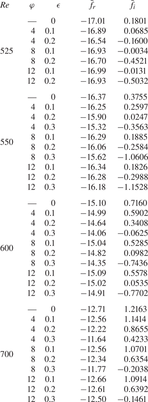
The temporal frequencies and growth rates computed for the two modulated flows, plotted in figures 13(c,d) and 13(e,f), again demonstrate that computations asymptote towards the same solution, irrespective of the radial position. However, as a consequence of the time-periodic modulation of the disk rotation rate, temporal frequencies  $f_r$ and growth rates $f_i$ are now characterised by oscillations. Over the span of each modulation cycle $T_m$, the temporal frequency $f_r$ displays periodic behaviour and oscillates about a value near that found for the steady disk. Moreover, the size of these oscillations increases with increasing modulation amplitude $\epsilon$. Similar fluctuations are observed in the temporal growth rates $f_i$, whereby during each modulation cycle, an interval of temporal decay ( $f_i<0$) is followed by a period of temporal growth ( $f_i>0$). The maximum and minimum values of the temporal growth rate $f_i$, during each modulation cycle, are respectively enhanced and reduced by increases in the modulation amplitude $\epsilon$. Averaging the temporal frequencies $f$ over one period of disk modulation establishes the mean frequencies $\bar {f}\approx -16.9+0.01\text {i}$ and $\bar {f}\approx -16.7-0.44\text {i}$ for the respective modulation amplitudes $\epsilon =0.1$ and $\epsilon =0.2$. (Mean calculations of $\bar {f}$ to greater accuracy are again tabulated in table 2.) Thus in the instance $\epsilon =0.1$, the mean temporal growth rate $\bar {f}_i$ is near critical conditions for absolute instability, while for $\epsilon =0.2$, strong temporal decay ensues.
The above analysis was extended to modulation frequencies  $\varphi =4$ and $12$. Linear disturbances were again excited impulsively for Reynolds number ${{Re}}=525$, with modulation amplitudes $\epsilon =0.1$ and $0.2$. Figure 14 displays the corresponding spatiotemporal disturbance development in the $(r,t/T)$-plane. Contour levels and the radial–temporal domain are equivalent to those presented for the modulation frequency $\varphi =8$ in figure 12, to help to draw comparisons. In both instances, time-periodic modulation again establishes a significant stabilising effect. Behaviour consistent with critical conditions for absolute instability is realised for amplitude $\epsilon =0.1$, while convectively unstable behaviour is achieved for $\epsilon =0.2$. On inspecting the disturbance maximum and behaviour of the respective trailing edges, it is clear that the modulation frequency $\varphi =12$ establishes a stabilising effect greater than that found for $\varphi =4$. Indeed, disturbance development obtained for $\varphi =12$ is commensurate with that brought about by modulating the disk at frequency $\varphi =8$. Additional temporal frequencies $\bar {f}$, obtained by averaging over one modulation cycle $T_m$, are included in table 2 for the above disturbances, alongside computations for several other Reynolds numbers ${{Re}}$.

Figure 14. Same as figure 12 for (a)  $\varphi =4$ and $\epsilon =0.1$, (b) $\varphi =12$ and $\epsilon =0.1$, (c) $\varphi =4$ and $\epsilon =0.2$, (d) $\varphi =12$ and $\epsilon =0.2$.
Further disturbances were simulated numerically for Reynolds number  ${{Re}}=550$, with modulation parameter settings $\epsilon =0.1,0.2$ and $\varphi =4,8,12$. Figure 15 displays the corresponding temporal frequencies $f_r$ and growth rates $f_i$ computed about the impulse centre $r_f={{Re}}$, with the modulation frequency $\varphi$ increasing monotonically down the figure. The illustration again demonstrates that time-periodic modulation establishes oscillations in both the temporal frequency and growth rate, with the periodicity governed by the modulation frequency $\varphi$ of the disk rotation rate. Additionally, larger modulation amplitudes $\epsilon$ enhance the size of these oscillations. However, the variation in the temporal frequency $f_r$ is found to decrease as the modulation frequency $\varphi$ increases, whereas fluctuations in the temporal growth rate $f_i$ appear to be less affected by the size of $\varphi$.

Figure 15. Temporal frequencies  $f_r$ and temporal growth rates $f_i$ for impulsively excited disturbances with $n=68$ and $r_f={{Re}}=550$. The temporal development is plotted about the radial position $r =r_f$, with the modulation amplitudes $\epsilon =0$ (solid lines), $\epsilon =0.1$ (dashed) and $\epsilon =0.2$ (dot-dashed), for (a,b) $\varphi =4$, (c,d) $\varphi =8$, and (e,f) $\varphi =12$.
The spatiotemporal development associated with the disturbances excited impulsively for Reynolds number  ${{Re}}=550$ and modulation frequency $\varphi =12$ are plotted in figures 16(a,c,e,g). In addition to modulation amplitudes $\epsilon =0,0.1,0.2$, the solution for $\epsilon =0.3$ is included in the illustration, while plots in figures 16(b,d,f,h) depict the equivalent behaviour for Reynolds number ${{Re}}=600$. The size of the modulation amplitude $\epsilon$ increases monotonically down the figure, while contour levels are now plotted on the logarithmic interval $\ln |\xi _{\theta,w}|\in [-1,14]$. The type of instability that develops in each instance is again identified by the direction of the leading and trailing edges of the disturbance wavepacket, i.e. upstream or downstream. Absolute instability is observed clearly for the modulation amplitude $\epsilon =0.1$ at both Reynolds numbers considered (figures 16c,d), as the leading and trailing edges propagate in opposite directions. Behaviour near critical conditions for absolute instability is found for $\epsilon =0.2$ and ${{Re}}=600$, as the trailing edge of the wavepacket is almost parallel to the time $t/T$-axis (figure 16f), while for the largest modulation amplitude, $\epsilon =0.3$, convectively unstable behaviour is demonstrated as both leading and trailing edges propagate radially outwards (figures 16g,h).

Figure 16. Spatiotemporal development of  $|\xi _{\theta,w}|$ for impulsively excited disturbances with $r_f={{Re}}$, $n=68$ and $\varphi =12$, for (a) ${{Re}}=550$ and $\epsilon =0$, (b) ${{Re}}=600$ and $\epsilon =0$, (c) ${{Re}}=550$ and $\epsilon =0.1$, (d) ${{Re}}=600$ and $\epsilon =0.1$, (e) ${{Re}}=550$ and $\epsilon =0.2$, (f) ${{Re}}=600$ and $\epsilon =0.2$, (g) ${{Re}}=550$ and $\epsilon =0.3$, (h) ${{Re}}=600$ and $\epsilon =0.3$. (Contour levels are plotted on the logarithmic interval $[-1,14]$.)
Tracing the changes in the contour shading in figure 16 demonstrates a significant reduction in the disturbance amplitude as the modulation amplitude  $\epsilon$ increases. The development of the maximum absolute value of the azimuthal perturbation field at the disk wall, $\max |\xi _{\theta,w}|$, is plotted in figures 17(a,c) for the disturbance wavepackets illustrated in figure 16, in addition to the results obtained for the modulation amplitude $\epsilon =0.4$. On normalising all disturbances to unity at time $t/T=0.1$, a huge reduction in the disturbance amplitude is realised by modulating the disk with amplitude $\epsilon =0.4$. For both Reynolds numbers modelled, $\max |\xi _{\theta,w}|$ is of the order $10^{1}$ at the end of one full rotation of the disk for $\epsilon =0.4$, while $\max |\xi _{\theta,w}|$ is of the order $10^{7}\unicode{x2013}10^{9}$ for the steady von Kármán flow. The corresponding radial trajectories $r_{max}$ of the amplitude maxima are plotted in figures 17(b,d), and indicate that the maximum of the disturbance convects further downstream as the modulation amplitude $\epsilon$ increases.

Figure 17. Development of the maximum value of  $|\xi _{\theta,w}|$ for disturbance wavepackets generated by impulsive excitation centred at $r_f={{Re}}$ for $n=68$ and variable modulation amplitudes $\epsilon$. (a,c) Magnitudes of the maxima; (b,d) radial trajectories of the amplitude maxima. The Reynolds number is ${{Re}}=550$ in (a,b), and ${{Re}}=600$ in (c,d). The modulation frequency is $\varphi =12$, and all disturbances are normalised so that they are equal to unity at $t/T=0.1$.
Figures 18(a,c,e) depict the variation in the mean temporal growth rate  $\bar {f}_i$ obtained for azimuthal mode number $n=68$, as a function of Reynolds number ${{Re}}$. Results are plotted for all three modulation frequencies modelled so far, i.e. $\varphi =4$, $8$ and $12$. Mean temporal growth rates were determined for Reynolds numbers ${{Re}}\in [500,700]$ at step intervals $\Delta {{Re}}=25$, with modulation amplitudes $\epsilon \in [0,0.3]$. Solutions further demonstrate the significant stabilising effect achieved via the application of time-periodic modulation to the disk rotation rate; mean temporal growth rates $\bar {f}_i$ decrease as $\epsilon$ increases and the onset of absolute instability is raised to larger Reynolds numbers. Moreover, modulation frequencies $\varphi =8$ and $12$ establish a reduction in the mean temporal growth rate greater than the results obtained for $\varphi =4$.

Figure 18. Mean temporal growth rates  $\bar {f}_i$ as functions of Reynolds number ${{Re}}$, with (a) $(n,\varphi )=(68,4)$, (b) $(n,\varphi )=(100,4)$, (c) $(n,\varphi )=(68,8)$, (d) $(n,\varphi )=(100,8)$, (e) $(n,\varphi )=(68,12)$, and (f) $(n,\varphi )=(100,12)$. The modulation amplitudes are $\epsilon =0$ (solid line), $\epsilon =0.1$ (dashed), $\epsilon =0.2$ (dot-dashed) and $\epsilon =0.3$ (dotted). Mean results are calculated by averaging $f_i$ over one full period of disk modulation at the radius $r=r_f={{Re}}$.
Comparable control of absolutely unstable behaviour was realised for other azimuthal mode numbers  $n$. For instance, figures 18(b,d,f) depict the equivalent set of computations for $n=100$, where absolute instability is again delayed to larger Reynolds number. Several mean temporal frequencies $\bar {f}=\bar {f}_r+\text {i}\bar {f}_i$ are given in tables 2 and 3, for the two azimuthal mode numbers $n=68$ and $n=100$, and modulation frequencies $\varphi =4,8,12$.
Table 3. Same as table 2 for  $n=100$.

The mean temporal growth rates  $\bar {f}_i$, shown in figure 18, are found to decrease proportionally with the square of the modulation amplitude $\epsilon$. This particular observation is illustrated for the modulation frequency $\varphi =8$ in figure 19(a) for $n=68$ and in figure 19(b) for $n=100$. Mean temporal growth rates are plotted as a function of the modulation amplitude $\epsilon$, for four fixed Reynolds numbers, ${{Re}} = 550$ to ${{Re}}=700$ at step intervals $\Delta {{Re}}=50$, with interpolation implemented to generate the curves of best fit. In each instance, solutions can be approximated by a parabolic function in $\epsilon$ of the form
 \begin{equation} \bar{f}_i=c_1\left(1-\left(\dfrac{\epsilon}{c_2}\right)^{2}\right), \end{equation}
where  $c_1$ is the temporal growth rate at $\epsilon =0$, and $c_2$ is the modulation amplitude associated with zero temporal growth. Thus a greater reduction in the temporal growth rate is realised as the modulation amplitude $\epsilon$ increases to larger values.

Figure 19. Mean temporal growth rates  $\bar {f}_i$ as functions of the modulation amplitude $\epsilon$ with frequency $\varphi =8$, and Reynolds numbers ${{Re}}=550$ (solid line), ${{Re}}=600$ (dashed), ${{Re}}=650$ (dot-dashed) and ${{Re}}=700$ (dotted), with azimuthal mode numbers (a) $n=68$, (b) $n=100$.
Critical Reynolds numbers  ${{Re}}_c$ for the onset of absolute instability can be estimated by applying linear interpolation to the mean temporal growth rates plotted in figure 18. Table 4 presents predictions for ${{Re}}_c$, for both azimuthal mode numbers $n=68$ and $n=100$. Calculations indicate that modulation frequencies $\varphi =8$ and $12$ raise the critical Reynolds number by approximately 70–85 units in the instance the modulation amplitude $\epsilon =0.2$, whereas a significantly smaller increase in ${{Re}}_c$ is realised for $\varphi =4$, at approximately 14–35 units when $\epsilon =0.2$.
Table 4. Predictions for the critical Reynolds number  ${{Re}}_c$ for azimuthal mode numbers $n=68$ and $n=100$. Calculations are based on applying linear interpolation to the solutions presented in figure 18.

Finally, modulation frequencies  $\varphi =4,8,12$ were chosen in this study to demonstrate the control benefits of disk modulation following the earlier observations of Morgan et al. (Reference Morgan, Davies and Thomas2021). In their Floquet analysis, Morgan and co-workers found that the control of stationary convective instabilities (both type I cross-flow and type II Coriolis) was optimised by modulation frequencies $8 \leq \varphi \leq 12$, with negligible control benefits realised for smaller and larger frequencies (see figure 7 of their paper). While extending the above study to other flow conditions and modulation settings would help to identify the optimal modulation configurations for controlling absolutely unstable behaviour, this was unfeasible due to the computational demands of the numerical scheme; a single numerical simulation, for fixed ${{Re}}$, $n$,
$n$,  $\epsilon$ and $\varphi$, required several computational processing hours. Undertaking a thorough investigation of all possible parameters was impractical, and instead the control benefits of modulating the disk rotation rate were presented for those azimuthal modes numbers that are considered to be the most significant on the steady rotating disk, namely $n=32$ for the cross-flow instability (Gregory et al. Reference Gregory, Stuart and Walker1955; Malik Reference Malik1986), and $n=68$ for absolute instability (Lingwood Reference Lingwood1995, Reference Lingwood1996). Nevertheless, further study was undertaken to ascertain whether the frequency range proposed by Morgan and co-workers was optimal for suppressing the temporal growth of absolutely unstable disturbances.
Figure 20 displays mean temporal growth rates  $\bar {f}_i$ as functions of the modulation frequency $\varphi$. Solutions are plotted for the two azimuthal mode numbers $n=68$ and $n=100$, in the instance the Reynolds number ${{Re}}=600$; these particular conditions correspond to strong absolutely unstable disturbances on the steady rotating disk. In addition, solutions are plotted for modulation amplitudes $\epsilon \in [0.1,0.3]$ and modulation frequencies $\varphi \in [2,30]$ at step intervals $\Delta \varphi =2$. Cross markers indicate the results obtained for these particular settings, with interpolation implemented to generate the curves of best fit. For the azimuthal mode number $n=68$, results indicate that the optimal frequency for suppressing the temporal growth rate, and the appearance of absolutely unstable behaviour, is found for $\varphi \approx 10$. For smaller and larger modulation frequencies, the effect on the temporal growth rate quickly diminishes, which is comparable with the behaviour found by Morgan and co-workers for the stationary cross-flow instability. Hence the preferred frequency is within the range of optimum frequencies suggested by Morgan et al. (Reference Morgan, Davies and Thomas2021). However, at the larger azimuthal mode number, solutions indicate that a frequency near $\varphi =14$ gives the optimal control benefits. Moreover, similar numerical simulations carried out for azimuthal mode numbers $n=75$, $85$ and $95$, suggest that control is optimised for frequencies $\varphi \approx 11$, $12$ and $13$, respectively. While results suggest that the preferred modulation frequency increases with the size of the azimuthal mode number, comparable reductions in the mean temporal growth rate $\bar {f}_i$ are still realised for $8\leq \varphi \leq 12$. Furthermore, the larger azimuthal mode numbers have not, to these authors’ knowledge, been observed to play a significant role in the laminar–turbulent transition process on a rotating disk. Hence the frequency range suggested by Morgan and co-workers, $8\leq \varphi \leq 12$, is the preferred modulation configuration for controlling both convective and absolute forms of linear instability.

Figure 20. Mean temporal growth rates  $\bar {f}_i$ as functions of the modulation frequency $\varphi$ with Reynolds number ${{Re}}=600$, and modulation amplitudes $\epsilon =0$ (solid line), $\epsilon =0.1$ (dashed), $\epsilon =0.2$ (dot-dashed) and $\epsilon =0.3$ (dotted), and azimuthal mode numbers (a) $n=68$, (b) $n=100$.
5. Conclusions
A numerical investigation has been undertaken on the development of linear disturbances in the time-periodic modulated rotating disk boundary layer. Modulation of the disk rotation rate was achieved in the manner outlined by Morgan et al. (Reference Morgan, Davies and Thomas2021), whereby sinusoidal motion was added to the otherwise constant disk rotation rate. In addition, the modulation amplitude  $\epsilon$ was limited to relatively small values to prevent the growth of stability mechanisms associated with the unsteady oscillations of the disk (Blennerhassett & Bassom Reference Blennerhassett and Bassom2002).
The study extends the recent Floquet stability analysis by Morgan et al. (Reference Morgan, Davies and Thomas2021) on the control of stationary convective instabilities, to encompass the effects of modulation on both convective and absolute forms of linear instability. Linear disturbance development was established using both a periodic and an impulsive wall forcing, for the unsteady base flow based on the radial homogeneous flow approximation; the radial dependence of the base flow was removed by replacing the radius  $r$ with the Reynolds number ${{Re}}$ in (2.9).
Periodic wall forcing was implemented to generate stationary disturbances associated with the convective cross-flow instability. Numerical simulations revealed behaviour consistent with the earlier Floquet analysis, with modulation establishing significant control benefits; the radial growth and amplitude of the stationary cross-flow instability were reduced.
Impulsive wall forcing was used to excite linear disturbance development for a range of flow and modulation settings, with a focus on the two azimuthal mode numbers  $n=32$ and $n=68$. These particular mode numbers respectively correspond to a strongly growing convective cross-flow instability and the critical value associated with the onset of absolute instability in the steady von Kármán flow. Time-periodic modulation of the disk rotation rate was found to establish a considerable stabilising effect for both the convective and absolute instabilities, which was illustrated via a reduction in both the disturbance amplitude and temporal growth rate (based on an averaging over one modulation period). Moreover, the onset of absolute instability was raised to larger Reynolds numbers ${{Re}}$ with the application of disk modulation. Thus it is expected that laminar–turbulent transition on the time-periodic modulated disk will be delayed to larger Reynolds numbers (or equivalently radial locations).
The strong stabilising effect brought about by modulating the disk rotation rate was enhanced by increasing the modulation amplitude  $\epsilon$, while modulation frequencies in the interval $8\leq \varphi \leq 12$ were found to bring about greater control benefits for the $n=68$ absolutely unstable mode. Negligible control benefits were realised for very small and large frequencies. This behaviour is consistent with the earlier Floquet analysis of Morgan et al. (Reference Morgan, Davies and Thomas2021), who found that frequencies in this parameter range optimised the control of the stationary cross-flow instability. For larger azimuthal mode numbers $n$, results suggest that the optimal modulation frequency increases with increasing $n$. However, as there is no evidence in the experimental literature that the larger $n$ modes play a role in laminar–turbulent transition on the steady rotating disk, we conclude that frequencies $8\leq \varphi \leq 12$ are the preferred modulation configuration for controlling both convective and absolute instabilities.
Finally, the current study has focused on the control of linear disturbances with the implementation of the radial homogeneous flow approximation. For the steady von Kármán flow, Davies & Carpenter (Reference Davies and Carpenter2003), Thomas & Davies (Reference Thomas and Davies2018) and Appelquist et al. (Reference Appelquist, Schlatter, Alfredsson and Lingwood2015) showed that the impulse response of linear disturbance development is affected by radial inhomogeneity, where the radial dependence of the base flow (2.9) is retained. For azimuthal mode numbers near critical conditions for absolute instability, convective characteristics dominate the global disturbance response (Davies & Carpenter Reference Davies and Carpenter2003), while at sufficiently large azimuthal mode numbers, a form of global instability emerges that is characterised by a faster than exponential growth (Thomas & Davies Reference Thomas and Davies2018). Thus we might expect radial inhomogeneity to have a similar effect on disturbance development in the modulated von Kármán flow. Additionally, nonlinearity and the subsequent stages of the transition process play an important role on the steady rotating disk (Pier Reference Pier2003, Reference Pier2007, Reference Pier2013; Appelquist et al. Reference Appelquist, Schlatter, Alfredsson and Lingwood2016, Reference Appelquist, Schlatter, Alfredsson and Lingwood2018) and can again be expected to become significant on the modulated rotating disk. Hence further investigation is required to understand the full effect of time-periodic modulation on laminar–turbulent transition in the rotating disk boundary layer.
Acknowledgements
We thank the referees for their helpful comments on this paper.
Funding
This work was supported by the UK Engineering and Physical Sciences Research Council.
Declaration of interests
The authors report no conflict of interest.
Appendix A. Checks on the numerical scheme
A.1. The radial and temporal step sizes
Figure 21 displays the temporal evolution of the disturbance at two successive radial locations  $r_f$ and $r_f+50$, where the disturbance was excited impulsively at $r_f=600$. The Reynolds number is ${{Re}}=600$, azimuthal mode number is $n=68$, and modulation parameter settings are $\epsilon =0.1$ and $\varphi =8$. Solutions are presented for three different numerical simulations, in which the radial and temporal step sizes, $\Delta r$ and $\Delta t$, have been varied. The aim here is to demonstrate that the choice for $\Delta r$ and $\Delta t$ used throughout this study is more than sufficient to compute accurately the development of linear disturbances in the rotating disk boundary layer with time-periodic modulation. The solid blue lines depict the results matched to $(\Delta r, \Delta t)=(1,0.5)$ that were used in the above investigation, while the dashed red and dotted yellow lines display the equivalent solutions obtained by scaling the respective temporal and radial step sizes by one-half. To graphical accuracy, the three numerical simulations are identical over the time interval shown. Moreover, the mean temporal growth rates $\bar {f}_i$ associated with the above numerical discretisations are found to be identical to at least two decimal places; see table 5.

Figure 21. Temporal evolution of the azimuthal vorticity perturbation field at the disk wall,  $\xi _{\theta,w}$, for impulsively excited disturbances with $n=68$ and $r_f={{Re}}=600$. The modulation amplitude is $\epsilon =0.1$, and frequency is $\varphi =8$. Solutions are plotted for radial and temporal step sizes $(\Delta r, \Delta t)=(1,0.5)$ (solid lines), $(\Delta r, \Delta t)=(1,0.25)$ (dashed) and $(\Delta r, \Delta t)=(0.5,0.5)$ (dotted), for (a) $r=r_f$, and (b) $r =r_f+50$. Here, $T =2{\rm \pi} {{Re}}$ is the non-dimensional time period for the disk rotation.
Table 5. Mean temporal frequencies  $\bar {f}_r$ and growth rates $\bar {f}_i$ for impulsively excited disturbances with $n=68$, ${{Re}}=600$, $\epsilon =0.1$ and $\varphi =8$. Mean results are calculated by averaging $f_r$ and $f_i$ over one full period of disk modulation about the radius $r=r_f={{Re}}$.

A.2. The influence of the domain size and outflow boundary condition
As discussed in § 3, condition (3.12) was imposed on all primary perturbation fields at the outer radial boundary to prevent the development of any spurious computational edge effects. In addition, the computational domain  $r_{{in}}\leq r \leq r_{{out}}$ was modelled sufficiently large, so that the outer radius $r_{{out}}$ was far removed from all disturbances that have evolved to an appreciable amplitude. Figure 22 displays the radial variation of the azimuthal vorticity perturbation field at the disk wall, $\xi _{\theta,w}$, for the flow conditions and modulation settings specified in § A.1. Solutions are plotted at times $t/T=1.15$ and $2.3$, for two numerical simulations with different outflow boundary locations. The solid blue lines depict the results obtained by setting $r_{{out}}=1300$, while the dashed red lines display the equivalent solution for $r_{{out}}=1500$. At the first time instant, shown in figure 22(a), the maximum of the disturbance wavepacket is located far away from the outer radial boundary, so the disturbance is negligible at the outflow in both cases. Unsurprisingly, the two solutions are identical. At the second time instant, plotted in figure 22(b), the disturbance amplitude at the outer radial boundary for the simulation undertaken on the shorter computational domain has achieved a size comparable to the wavepacket maximum, whereas for the numerical simulation conducted on the longer computational domain, the disturbance amplitude is again negligible at the outflow. Nevertheless, there is still excellent agreement between the two computations, and there is no indication that the shorter computational domain has generated any spurious numerical noise.

Figure 22. Instantaneous radial variation of the azimuthal vorticity perturbation field at the disk wall,  $\xi _{\theta,w}$, for impulsively excited disturbances with $n=68$ and $r_f={{Re}}=600$. The modulation amplitude is $\epsilon =0.1$, and frequency is $\varphi =8$. The outer radial boundary is fixed at $r_{out}=1300$ (solid lines) and $r_{out}=1500$ (dashed), for (a) $t/T=1.15$, and (b) $t/T=2.3$.
A.3. Duration of the initial impulse
In the above impulse response analysis, where disturbance development was established by an impulsive wall motion (4.1c), the duration of the initial impulse was fixed by the parameter  $\sigma$. Setting $\sigma =1/(20{\rm \pi} ^{2})$ was found to initially excite an extensive range of frequencies, after which the most unstable mode dominated the flow response. Other $\sigma$ values were considered in the early testing of the numerical formulation but did not affect the general response of the disturbances. For instance, figure 23 depicts the temporal evolution of $\xi _{\theta,w}$ for flow conditions $n=68$ and $r_f={{Re}}=600$, and modulation settings $\epsilon =0.1$ and $\varphi =8$. Solutions are plotted for three numerical simulations with different $\sigma$ values. The solid blue line displays the result generated for $\sigma =1/(20{\rm \pi} ^{2})$, while the dashed red and dotted yellow lines depict solutions matched to $\sigma =1/(40{\rm \pi} ^{2})$ and $\sigma =1/(2{\rm \pi} ^{2})$, respectively. These two latter simulations respectively establish longer and shorter initial impulses than the value of $\sigma$ used in the above investigation. However, on normalising all three solutions at time $t/T=0.1$, the resulting temporal evolution is identical in all three cases; each disturbance grows with the same periodicity and displays absolutely unstable behaviour, i.e. the disturbance grows with increasing time. Thus the impulse response is unaffected by the initial duration of the impulsive wall forcing.

Figure 23. Temporal evolution of the azimuthal vorticity perturbation field at the disk wall,  $\xi _{\theta,w}$, for impulsively excited disturbances with $n=68$ and $r_f={{Re}}=600$. The modulation amplitude is $\epsilon =0.1$, and frequency is $\varphi =8$. Solutions are plotted for an initial impulse $\sigma =1/(20{\rm \pi} )^{2}$ (solid lines), $\sigma =1/(40{\rm \pi} )^{2}$ (dashed) and $\sigma =1/(2{\rm \pi} )^{2}$ (dotted). Solutions are normalised to unity at $t/T=0.1$.
Appendix B. Variation in the phase of the unsteady flow
Time-periodic modulation of the rotating disk was achieved by imposing an unsteady disk rotation rate
 \begin{equation} \varOmega^{*}(t^{*}) = \varOmega_0^{*} + \lambda\phi^{*}\cos(\phi^{*}t^{*}-{\rm \pi}/2); \end{equation}
recall (2.2). The first term represents a constant disk rotation rate, while the second term establishes modulation of the rotating disk. In the above study, the  ${\rm \pi} /2$ phase shift was implemented to ensure that time zero corresponds to the von Kármán flow conditions. Consequently, the oscillations observed in the disturbance development, illustrated in figures 7–9 and 11–16, were dependent on this particular choice of phase shift. Nevertheless, equivalent stability characteristics were obtained for disturbances excited impulsively about other phases of the periodic motion.
Generalising the disk rotation rate  $\varOmega ^{*}$ as
 \begin{equation} \varOmega^{*}(t^{*}) = \varOmega_0^{*} + \lambda\phi^{*}\cos(\phi^{*}t^{*}+\gamma), \end{equation}
for a phase shift  $\gamma$ (where $\gamma =-{\rm \pi} /2$ recovers the flow modelled herein), several disturbances were simulated numerically to demonstrate the effect of varying the initial phase of the impulsive forcing. Figure 24(a) displays the temporal evolution of the envelopes $|\xi _{\theta,w}|$ at $r=r_f$, established for flow settings ${{Re}}=525$ and $n=68$, and modulation parameter settings $\varphi =8$ and $\epsilon =0.1$. Solutions are plotted for four phase shifts $\gamma$: the solid blue line corresponds to $\gamma =-{\rm \pi} /2$ modelled throughout this study, while the red dashed, yellow dot-dashed and purple dotted lines depict the respective solutions for $\gamma =0$, ${\rm \pi} /2$ and ${\rm \pi}$. As expected, all four solutions are characterised by oscillatory behaviour, with disturbances attaining local maxima and minima at different time instances. The perturbation matched to $\gamma =0$ achieves a local maximum (minimum) at the same point in time that the $\gamma ={\rm \pi}$ disturbance attains a local minimum (maximum). Similarly for the $\gamma =\pm {\rm \pi}/2$ time history envelopes. Moreover, behaviour consistent with critical absolute instability is emerging in each instance, as for large time $t$, disturbances neither grow nor decay from one period of disk modulation to the next. However, there is a noticeable difference in the respective amplitudes of each disturbance. Solutions established for phase shifts $\gamma =0$ and ${\rm \pi} /2$ attain amplitudes (both maximum and minimum) larger than those amplitudes realised for $\gamma =-{\rm \pi} /2$ and ${\rm \pi}$. This particular observation is a direct consequence of the phase in which disturbances are excited initially; the amplitude of the disturbance varies with the phase shift $\gamma$.

Figure 24. Variation in the initial phase  $\gamma$ of the unsteady base flow, for impulsively excited disturbances with $n=68$, $r_f={{Re}}=525$, $\epsilon =0.1$ and $\varphi =8$. (a) Temporal evolution of the envelopes $|\xi _{\theta,w}|$ at $r=r_f$. (b) Temporal evolution of the radial location $r_{{te}}$ of the trailing edge, associated with the spatiotemporal disturbance development, with solutions normalised to unity at $t/T=0.1$.
The spatiotemporal disturbance development associated with the above numerical simulations was constructed in the  $(r,t/T)$-plane, with all four solutions normalised at $t/T=0.1$. The respective leading and trailing edges of each disturbance were then determined by defining contour levels on the logarithmic interval $\ln |\xi _{\theta,w}|=[-1,12]$ (as implemented in figure 12). Figure 24(b) displays the temporal evolution of the radial location $r_{{te}}$ associated with the four trailing edges (based on the contour level $\ln |\xi _{\theta,w}|=-1$), with line types the same as those given in figure 24(a). For each phase shift $\gamma$, the trailing edge is found to oscillate about the radial position $r=532$ for large time $t/T$. Meanwhile, the corresponding leading edges are found to propagate radially outwards with a comparable non-zero velocity. Thus behaviour consistent with the onset of absolute instability develops in each instance. Hence despite the obvious differences in the disturbance amplitude, illustrated in figure 24(a), qualitatively similar stability characteristics (that is, critical absolute instability) are realised.


 Open access