2. Equations of motion

A flat plate of width $L$, immersed in a viscous fluid of viscosity $\mu$ and constant density $\rho$, settles onto a flat horizontal surface. We consider the two-dimensional case, where the gap $h$ between both surfaces depends only upon one Cartesian coordinate of the plane ($x$, say), and is independent of $y$. It is also assumed that the plate is sufficiently wide that fluid motion in the $y$-direction can be neglected.

Consider the horizontal component of the two solid surface velocities to be $v_1(t)$ (lower surface) and $v_2(t)$ (upper). We assume that the separation between both surfaces $h(x,t)$ is sufficiently small that lubrication theory applies. In particular, if the typical separation length is $\bar {h}$, we assume that $\bar {h}\ll L$. Defining a dimensionless parameter $\varepsilon = \bar {h}/L\ll 1$, we then have that the inclination angle $\theta \sim O(\varepsilon )\ll 1$. We also assume that the fluid velocities in the gap are sufficiently small that the Reynolds number, ${Re}$, is extremely small. Under these conditions, we have, locally, Poiseuille flow in a gap with a slowly varying width, which is the assumption underlying the formulation of lubrication theory. The assumption that the Reynolds number is small may be validated by computing the flow rate, finding that ${Re}$ approaches zero as the gap decreases.

In lubrication theory, both the lift and drag forces arise from regions where the gap $h$ is very small, and the forces are, therefore, expected to be proportional to $L$. There is a small region at the edge of the plate, where the Poiseuille flow approximation is not valid. In this region, with width of order $h$, the velocity gradients rapidly reduce from the large values in the lubrication layer to the much lower values which occur in other regions of the flow. These considerations indicate that the fractional error which arises when estimating forces using lubrication theory is $O(\varepsilon )$.

The assumption that there is a Poiseuille flow in the gap implies that the volume flux per unit depth is $J(x,t)$, and the flux and pressure $p$ are related by

(2.1)\begin{equation} J=\left(\frac{v_1+v_2}{2}\right)h-\frac{h^3}{12\mu}\frac{\partial p}{\partial x} , \end{equation}

and the continuity equation is

(2.2)\begin{equation} \frac{\partial h}{\partial t}+\frac{\partial J}{\partial x}=0 . \end{equation}

Poiseuille flow also implies that the tangential stress on the upper surface is

(2.3)\begin{equation} \sigma=-\mu\left(\frac{v_2-v_1}{h}\right)-\frac{h}{2}\frac{\partial p}{\partial x} . \end{equation}

We can use these equations in any convenient Cartesian frame. Rather than using the laboratory frame, let us use a frame that is attached to the plate. The displacement of the left-hand edge of the plate relative to some fixed position in the laboratory frame is $X(t)$. The velocity of the upper bounding surface in the plate frame is then $v_2=0$, and the velocity of the lower surface is $v_1=-\dot {X}$. The configuration of the plate is then described by specifying height at displacement $x$ from the left edge:

(2.4)\begin{equation} h(x,t)=Z(t)+\theta(t)x, \end{equation}

where $Z(t)$ is the gap between the left-hand edge of the plate and the surface, and $\theta (t)$ is the angle between the plate and the horizontal, see figure 1.

We wish to determine the force components in the vertical and horizontal direction, $F_z$ and $F_x$, respectively, and torque $G$ on the plate. These are

(2.5a)$$\begin{gather} F_z=\int_0^L {\rm d}\kern 0.7pt x\,p=p_0L-\int_0^L{\rm d}\kern 0.7pt x\,x\frac{\partial p}{\partial x}, \end{gather}$$

(2.5b)$$\begin{gather}F_x=\int_0^L{\rm d}\kern 0.7pt x\,\sigma -\theta F_z=-\mu\int_0^L{\rm d}\kern 0.7pt x\,\frac{\dot{X}}{h} -\int_0^L{\rm d}\kern 0.7pt x\,\frac{h}{2}\frac{\partial p}{\partial x} -\theta F_z, \end{gather}$$

(2.5c)$$\begin{gather}G=\int_0^L{\rm d}\kern 0.7pt x\,xp=-\int_0^L{\rm d}\kern 0.7pt x\,\frac{x^2}{2}\frac{\partial p}{\partial x}, \end{gather}$$

where $p_0 = p(0)$. The above expressions depend on the pressure gradient $\partial p/\partial x$, which we can determine from (2.1) as follows. Inserting (2.4) into the continuity equation (2.2) and integrating once we obtain

(2.6)\begin{equation} J=J_0-\dot{Z}x-\frac{\dot{\theta}}{2}x^2, \end{equation}

where $J_0$ is a constant. It will be useful to define

(2.7)\begin{equation} I^n_m=\int_0^L{\rm d}\kern 0.7pt x\,\frac{x^n}{h^m}. \end{equation}

We can now find the pressure gradient

(2.8)\begin{equation} \frac{\partial p}{\partial x}=12\mu\left[\dot{Z}\frac{x}{h^3}+ \frac{\dot{\theta}}{2}\frac{x^2}{h^3}-\frac{\dot{X}}{2}\frac{1}{h^2}-J_0\frac{1}{h^3}\right], \end{equation}

where $J_0$ is found by integrating the above expression and imposing that $p(L)=p(0)$:

(2.9)\begin{equation} J_0=\frac{1}{I^0_3}\left[\dot{Z}I^1_3+\frac{\dot{\theta}}{2}I^2_3-\frac{\dot{X}}{2}I^0_2\right]. \end{equation}

Provided the background pressure is high enough to prevent cavitation, its value must be irrelevant, so we set $p_0=0$. Therefore, the force components are

(2.10a)$$\begin{gather} F_z=\frac{12\mu}{I^0_3}\left[\dot{X}\frac{1}{2}\big(I^0_3I^1_2-I^0_2I^1_3\big)+\dot{Z} \big(I^1_3I^1_3-I^2_3I^0_3\big)+\dot{\theta}\frac{1}{2}\big(I^1_3I^2_3-I^3_3I^0_3\big)\right] , \end{gather}$$

(2.10b)$$\begin{gather}F_x=\frac{12\mu}{I^0_3}\left[\dot{X}\left(\frac{1}{6}I^0_1I^0_3-\frac{1}{4}I^0_2I^0_2\right) +\dot{Z}\frac{1}{2}\big(I^1_3I^0_2-I^1_2I^0_3\big)+\dot{\theta} \frac{1}{4}\big(I^0_2I^2_3-I^2_2I^0_3\big)\right]-\theta F_z, \end{gather}$$

(2.10c)$$\begin{gather}G=\frac{12\mu}{I^0_3}\left[\dot{X}\frac{1}{4}\big(I^2_2I^0_3-I^2_3I^0_2\big) +\dot{Z}\frac{1}{2}\big(I^1_3I^2_3-I^3_3I^0_3\big) +\dot{\theta}\frac{1}{4}\big(I^2_3I^2_3-I^4_3I^0_3\big)\right]. \end{gather}$$

We can write the relation between forces and velocities in terms of a matrix:

(2.11)\begin{equation} (F_x+\theta F_z,F_z,G)^{\rm T}=\frac{6\mu}{I^0_3}{\boldsymbol{\mathsf{A}}}(\dot{X},\dot{Z}, \dot{\theta})^{\rm T} \end{equation}

where the matrix ${\boldsymbol{\mathsf{A}}}$ is

(2.12) \begin{equation} {\boldsymbol{\mathsf{A}}}= \left(\begin{array}{@{}ccc@{}} \dfrac{1}{3}I^0_1I^0_3-\dfrac{1}{2}I^0_2I^0_2 & I^0_2I^1_3-I^1_2I^0_3 & \dfrac{1}{2}\left(I^0_2I^2_3-I^2_2I^0_3\right) \\ I^1_2I^0_3-I^1_3I^0_2 & 2\left(I^1_3I^1_3-I^2_3I^0_3\right) & I^1_3I^2_3-I^3_3I^0_3 \\ \dfrac{1}{2}\left(I^2_2I^0_3-I^0_2I^2_3\right) & I^1_3I^2_3-I^3_3I^0_3 & \dfrac{1}{2}\left(I^2_3I^2_3-I^4_3I^0_3\right) \end{array} \right). \end{equation}

(Note that our definitions do not imply that this matrix need be symmetric, but it may be possible to obtain a symmetric matrix using an alternative formulation of the problem.) Equations of motion in which a generalised velocity vector is obtained from a generalised force vector by matrix multiplication occur quite generally in treatments of viscosity dominated flow, and the matrix ${\boldsymbol{\mathsf{A}}}$ is termed the resistance matrix (Happel & Brenner Reference Happel and Brenner1983). The equations of motion derived in Cawthorn & Balmforth (Reference Cawthorn and Balmforth2010) were obtained in a slightly different form, compared with our (2.11) and (2.12), but they are consistent with our formulation.

3. Dimensionless equations

It will be efficient to define non-dimensional dynamical variables,

(3.1a–c)\begin{equation} \eta=\frac{L\theta}{Z} ,\quad\zeta=\frac{X}{L} ,\quad\xi=\frac{Z}{L} , \end{equation}

and a non-dimensional version of the integrals $I^n_m$,

(3.2)\begin{equation} I^n_m=\frac{L^{n+1}}{Z^m}K^n_m(\eta), \end{equation}

with

(3.3)\begin{equation} K^n_m(\eta)=\int_0^1 {\rm d}u\,\frac{u^n}{(1+\eta u)^m}. \end{equation}

With these definitions the generalised force components are expressed in terms of the dimensionless dynamical variables as follows:

(3.4a)\begin{align} F_z&=\frac{6\mu L}{K^0_3}\left[\frac{\dot{\zeta}}{\xi^2}\big(K^1_2K^0_3-K^1_3K^0_2\big) +\frac{\dot{\xi}}{\xi^3}\left[\big(2K^1_3K^1_3-2K^0_3K^2_3\big)+\eta\big(K^1_3K^2_3-K^3_3K^0_3\big)\right]\right. \nonumber\\ &\quad +\left.\frac{\dot \eta}{\xi^2}\big(K^1_3K^2_3-K^0_3K^3_3\big)\right] , \end{align}

(3.4b) \begin{align} F_x+\theta F_z&=\frac{6\mu L}{K^0_3} \left[\frac{\dot{\zeta}}{\xi}\left(\frac{1}{3}K^0_1K^0_3-\frac{1}{2}K^0_2K^0_2\right) +\frac{\dot{\xi}}{\xi^2}\left[\vphantom{\frac{1}{2}}\big(K^0_2K^1_3-K^1_2K^0_3\big)\right.\right.\nonumber\\ &\quad + \left.\left.\eta\left(\frac{1}{2}K^0_2K^2_3-\frac{1}{2}K^2_2K^0_3\right) \right] +\frac{\dot \eta}{\xi}\left(\frac{1}{2}K^0_2K^2_3-\frac{1}{2}K^2_2K^0_3\right)\right], \end{align}

(3.4c)\begin{align} G&=\frac{6\mu L^2}{K^0_3}\left[\frac{\dot{\zeta}}{\xi^2}\left(\frac{1}{2}K^2_2K^0_3-\frac{1}{2}K^2_3K^0_2\right)+ \frac{\dot{\xi}}{\xi^3}\left[\vphantom{\frac{1}{2}}\big(K^2_3K^1_3-K^3_3K^0_3\big)\right.\right. \notag\\ &\quad + \left.\left.\eta \left(\frac{1}{2}K^2_3K^2_3 -\frac{1}{2}K^4_3K^0_3\right)\right] +\frac{\dot \eta}{\xi^2}\left(\frac{1}{2}K^2_3K^2_3-\frac{1}{2}K^4_3K^0_3\right) \right] . \end{align}

It will also be helpful to introduce another dimensionless variable $\lambda$ that can be used in place of $\xi$, defined by

(3.5)\begin{equation} \lambda=\ln \xi. \end{equation}

Then the force equations are

(3.6a)$$\begin{gather} F_x=\frac{\mu L}{\xi}\left[B_{11}(\eta)\dot{\zeta}+B_{12}(\eta)\dot{\lambda}+B_{13}(\eta)\dot{\eta}\right], \end{gather}$$

(3.6b)$$\begin{gather}F_z=\frac{\mu L}{\xi^2}\left[B_{21}(\eta)\dot{\zeta}+B_{22}(\eta)\dot{\lambda}+B_{23}(\eta)\dot{\eta}\right], \end{gather}$$

(3.6c)$$\begin{gather}G=\frac{\mu L^2}{\xi^2}\left[B_{31}(\eta)\dot{\zeta}+B_{32}(\eta)\dot{\lambda}+B_{33}(\eta)\dot{\eta}\right], \end{gather}$$

where the coefficients $B_{ij}(\eta )$ are obtained by comparison with (3.4), e.g.

(3.7)\begin{equation} B_{11}(\eta)=\frac{2K^0_1K^0_3-3K^0_2K^0_2}{K^0_3}-6\eta \frac{K^1_2K^0_3-K^1_3K^0_2}{K^0_3}. \end{equation}

The equations of motion can then be expressed in the form

(3.8)\begin{equation} \frac{\xi^2}{\mu L} \left(\begin{array}{@{}c@{}} F_x/\xi \\ F_z\\ G/L \end{array}\right) ={\boldsymbol{\mathsf{B}}} \left(\begin{array}{@{}c@{}} \dot \zeta \\ \dot \lambda \\ \dot \eta \end{array}\right). \end{equation}

We are interested in settling of the body due to a gravity force $W$, that is, in the vertical direction, and acts through a point $x=sL$ from the left-hand edge, so the opposing forces on the body due to the fluid are $(F_x,F_z,G)=(0,W,sWL)$. Introduce a transformed time variable $\tau$, which satisfies

(3.9)\begin{equation} \frac{{\rm d}\tau}{{\rm d}t}=\frac{\xi^2W}{\mu L} \end{equation}

so that, if the inverse of ${\boldsymbol{\mathsf{B}}}(\eta )$ is ${\boldsymbol{\mathsf{C}}}(\eta )$, then (3.8) becomes

(3.10) \begin{equation} \left(\begin{array}{@{}c@{}} \dfrac{{\rm d}\zeta}{{\rm d}\tau} \\ \dfrac{{\rm d}\lambda }{{\rm d}\tau}\\ \dfrac{{\rm d}\eta}{{\rm d}\tau} \end{array}\right) ={\boldsymbol{\mathsf{C}}} \left(\begin{array}{@{}c@{}} F_x /W \xi \\ F_z/W \\ G/WL \end{array}\right) = {\boldsymbol{\mathsf{C}}}\left(\begin{array}{@{}c@{}} 0 \\ 1 \\ s \end{array}\right) . \end{equation}

For our settling plate we then have the following equations of motion:

(3.11a)$$\begin{gather} \frac{{\rm d}\zeta}{{\rm d}\tau}=C_{12}(\eta)+sC_{13}(\eta)\equiv F_\zeta(\eta,s), \end{gather}$$

(3.11b)$$\begin{gather}\frac{{\rm d}\lambda}{{\rm d}\tau}=C_{22}(\eta)+sC_{23}(\eta)\equiv F_\lambda(\eta,s), \end{gather}$$

(3.11c)$$\begin{gather}\frac{{\rm d}\eta}{{\rm d}\tau}=C_{32}(\eta)+sC_{33}(\eta)\equiv F_\eta(\eta,s). \end{gather}$$

The matrix elements of ${\boldsymbol{\mathsf{B}}}(\eta )$ and ${\boldsymbol{\mathsf{C}}}(\eta )$ can be determined analytically: the expressions are given in Appendix A.

It is possible to find solutions in which $Z(t)$ is increasing, but the height of the centre of gravity must always decrease monotonically. It is not obvious that (3.11a)–(3.11c) have this property. Appendix B demonstrates that this property holds.

4. Solution of dimensionless equations

In § 4.2 it will be shown that the equations of motion (3.11) can be solved, expressing $t$, $\xi$ and $\zeta$ as functions of $\eta$, defined as integrals of elementary functions. These exact solutions are, however, quite difficult to interpret. It is the qualitative behaviour of the solutions that is usually of more interest than precise expressions. In particular, it is desirable to understand whether the edge of the plate makes contact in finite time, or whether the angle of the plate decreases so that it settles without ever making contact. This is addressed in the next § 4.1, before we consider the exact solution.

4.1. Fixed points

The qualitative form of the solution is addressed by looking at the dynamics of the dimensionless variable $\eta$. If the left-hand edge makes contact, this corresponds to $\eta \to \infty$ (and a contact of the right-hand edge is $\eta \to -1$).

Consider (3.11c). This is a differential equation for $\eta (\tau )$ that is independent of the other variables. Any fixed points (nullclines) of the $\eta (\tau )$ dynamics are determined by the condition

(4.1)\begin{equation} F_\eta(\eta^\ast,s)=0 . \end{equation}

This determines a fixed point $\eta ^\ast (s)$ as a function of the position of the centre of gravity, $s$. The fixed point is stable if

(4.2)\begin{equation} \kappa(s)\equiv-\frac{\partial F_\eta}{\partial \eta}(\eta^\ast(s),s)>0, \end{equation}

(and, conversely, unstable if $\kappa <0$). The matrix elements quoted in (A2) of Appendix B enable us to express $F_\eta (\eta,s)$ in terms of elementary functions: we find that the values of $s$ and $\eta$ at a fixed point are related by

(4.3)\begin{equation} s=\frac {2\left(\ln \left( \eta+1 \right) \right)^2(\eta+1)+\ln \left( \eta+1\right)\eta(\eta+1)-3\eta^2} {\ln \left(\eta+1\right) \eta^2} . \end{equation}

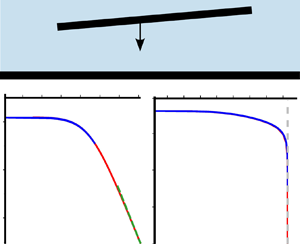
Figure 2 shows plots of $F_\eta (\eta,s)$ as a function of $\eta$ for different values of $s$. Because fixed points were found with widely differing values of $\eta$, the plots of figure 2 correspond to four different ranges of $\eta$. Figure 2(a) illustrates the limit:

(4.4)\begin{equation} \lim_{\eta\to -1}F_\eta(\eta,s)=0, \end{equation}

i.e. $\eta =-1$ (right-hand edge approaches contact) is a fixed point for all $s$. By symmetry, the limit $\eta \to \infty$ (i.e. left-hand edge approaches contact) can also be regarded as a fixed point. However, the function $F_\eta (\eta,s)$ has a singular form as $\eta \to -1$, and the dynamics in the vicinity of these edge-contact fixed points is highly unusual. In § 6 we consider in some detail the case where the edge is close to contact. There we argue that the plate makes contact in finite time.

Figure 2. Plot of $F_\eta (\eta,s)$ as a function of $\eta$ for different choices of the centre of mass position, $s$, and for four different ranges of $\eta$. Attractive fixed points of $\eta$ occur where $F_\eta =0$ and $F'_\eta <0$.

Figures 2(b)–2(d) show the behaviour of $F_\eta$ for three different ranges of $\eta$ as we increase its value above $\eta =-1$. We can see how fixed points are found at increasingly large values of $\eta$. It would be instructive to plot a phase diagram that shows the locations of the stable and unstable fixed points as lines in the $(\eta,s)$ plane, but the fact that $\eta$ may approach infinity is inconvenient. There is a left–right symmetry of the system, such that a fixed point at $(\eta,s)$ should be reflected as a fixed point with the same stability at $(-\eta /(1+\eta ),1-s)$. If we were to use an alternative dimensionless parameter,

(4.5)\begin{equation} \phi=\frac{\eta}{2+\eta} \end{equation}

to describe the configuration of the plate, then the configuration space extends from $\phi =-1$ (right-hand edge in contact) to $\phi =+1$ (left-hand edge in contact), and a fixed point at $(\phi,s)$ is mirrored by one at $(-\phi,1-s)$. In terms of the symmetrised configuration variable $\phi$, the equation for the fixed points is

(4.6)\begin{equation} s={\mathcal{S}}(\phi)\equiv \left(\frac{1-\phi^2}{2\phi^2}\right)\ln \left(\frac{1+\phi}{1-\phi}\right) +\left(\frac{1+\phi}{2\phi}\right) -\frac{3}{\ln \left(\dfrac{1+\phi}{1-\phi}\right)} . \end{equation}

The function ${\mathcal {S}}(\phi )$ satisfies the symmetry relation

(4.7)\begin{equation} {\mathcal{S}}(\phi)+{\mathcal{S}}(-\phi)=1 . \end{equation}

Figure 3 shows the phase diagram of the system using the $(\phi,s)$ coordinates. If we include the stable fixed points at $\phi =\pm 1$, there are either three or five fixed points, depending upon the value of $s$ (the centre of mass position).

1. (i) For $0< s<0.3764208755\ldots$ there is an unstable fixed point at a value of $\phi ^\ast$ that is very close to the point at which the right-hand side touches (note the dashed red line and solid horizontal blue lines are indistinguishable in figure 3). In this range of $s$, $\phi ^\ast$ lies in $(-1,-0.999206\ldots\,]$. If the right-hand edge is exquisitely close to making contact, it does so. Otherwise, we expect that the left-hand edge will make contact. In § 6 we argue that, in both cases, contact happens in finite time.

2. (ii) For $1>s>0.623579125\ldots\,$, the situation is the mirror image of the case $0< s<0.3764208755\ldots\,$. There is an unstable fixed point at a value of $\phi ^\ast$ that lies in the interval $[0.999206\ldots,1)$. If $\phi$ is initially greater than $\phi ^\ast$, the left-hand edge contacts in finite time. If $\phi$ is less than $\phi ^\ast$ (which is the only case that is of practical relevance), the right-hand edge contacts in finite time.

3. (iii) There is a region in the interval $0.3764208755\ldots \leq s\leq 0.6235791253\ldots$ that has two stable fixed points at $\phi =\pm 1$, two unstable fixed points, and one other stable fixed point between the unstable fixed points. There is a basin of attraction for which the value of $\phi$ approaches the non-trivial stable fixed point $\phi ^\ast (s)$. This stable fixed point starts at $\phi ^\ast (0.3764208755\ldots )=0.83774254\ldots\,$, passes through $\phi ^\ast (1/2)=0$, and disappears at $\phi ^\ast (0.6235791253\ldots )=-0.83774254\ldots\,$. The basin of attraction in the $\phi$ variable is at its largest when $s=1/2$. At this point, the unstable fixed points are at $\phi =\pm 0.9956216$, and all initial conditions in between these values converge to the plate settling in the flat, $\phi =0$, configuration.

Figure 3. Plot showing fixed points in phase space of model, using $\phi$, defined by (4.5) and (3.1a–c), to describe the configuration of the plate, and $s$ to parametrise the position of its centre of gravity. The blue line indicates stable fixed points, the red line indicates unstable fixed points.

There does not appear to be any reason to anticipate that the phase diagram of the system should be this complicated. In § 5 we show that the approach to the stable fixed point has a power-law dependence upon time $t$. The unstable fixed points drive $\phi$ towards $\pm 1$, that is, towards one of the edges contacting the fixed baseplate. In § 6.1 we show, when an edge is sufficiently close, contact occurs in finite time, and § 6.2 considers the subsequent motion.

4.2. Exact solution

We define a dimensionless time variable

(4.8)\begin{equation} \tilde{t}=\frac{Wt}{\mu L}\xi_0^2, \end{equation}

where $\xi _0$ is the initial value of $Z/L$. Equations (3.9) and (3.11) then lead to the following differential equations for $\tilde {t}(\eta )$, $\lambda (\eta )$ and $\zeta (\eta )$:

(4.9a)$$\begin{gather} \frac{{\rm d}\tilde{t}}{{\rm d}\eta} =\xi_0^2\frac{\exp[-2\lambda(\eta,s)]}{F_\eta(\eta,s)}, \end{gather}$$

(4.9b)$$\begin{gather}\frac{{\rm d}\lambda}{{\rm d}\eta}=\frac{F_\lambda(\eta,s)}{F_\eta(\eta,s)}, \end{gather}$$

(4.9c)$$\begin{gather}\frac{{\rm d}\zeta}{{\rm d}\eta}=\frac{F_\zeta(\eta,s)}{F_\eta(\eta,s)}. \end{gather}$$

These three differential equations can be integrated to express $t$, $\lambda =\ln \xi$ and $\zeta$ as functions of $\eta$, for example (4.9a) gives

(4.10)\begin{equation} t=\frac{\mu L}{W}\int_{\eta_0}^\eta {\rm d}\eta'\,\frac{\exp[-2\lambda(\eta')]}{C_{32}(\eta')+sC_{33}(\eta')} \end{equation}

where $\lambda (\eta )$ is found by integrating (4.9b):

(4.11)\begin{equation} \lambda(\eta)-\lambda(\eta_0)=\int_{\eta_0}^\eta {\rm d}\eta'\,\frac{C_{22}(\eta')+sC_{23}(\eta')}{C_{32}(\eta')+sC_{33}(\eta')} . \end{equation}

These expressions give an exact expression for $t$ in terms of integrals of elementary functions of $\eta$, but they are too complicated to be instructive. Furthermore, in order to express $Z$, $\theta$ and $X$ as functions of $t$, it is necessary to invert the function $t(\eta )$ defined by (4.10) and (4.11).

5. Asymptotic solution near stable fixed point

If the initial conditions are in the basin of attraction of a stable fixed point $\eta ^\ast (s)$, then the long-time behaviour of the solution is determined by the solution in the vicinity of this fixed point.

If $\eta$ is close to $\eta ^\ast$, then

(5.1)\begin{equation} \frac{{\rm d} \eta}{{\rm d} \tau} = F_\eta(\eta,s) \approx F_\eta(\eta^\ast,s) + (\eta - \eta^\ast) F'_\eta(\eta^\ast,s) =- (\eta - \eta^\ast) \kappa(s) , \end{equation}

so, with $\eta _0 = \eta (0)$, the solution of (3.11c) is approximated by

(5.2)\begin{equation} \eta(\tau)\sim \eta^\ast+[\eta_0-\eta^\ast]\exp[-\kappa(s)\tau], \end{equation}

where $\kappa (s)$ was defined in (4.2). When $\eta (\tau )$ converges to this stable fixed point at $\eta ^\ast$, the functions $F_\zeta$ and $F_\lambda$ in (3.11a), (3.11b) approach constant values. Equation (3.11b) then implies that

(5.3)\begin{equation} \xi(\tau)\sim \xi_0 \exp[F_\lambda(\eta^\ast,s)\tau], \end{equation}

and hence (3.9) can be integrated to give $t$ as a function of $\tau$ and $\xi _0$:

(5.4)\begin{align} t&= \frac{\mu L}{W}\int_0^\tau {\rm d}\tau'\,\xi^{-2}(\tau') \nonumber\\ &\sim\frac{\mu L}{W\xi_0^2}\int_0^\tau {\rm d}\tau'\,\exp[-2F_\lambda(\eta^\ast,s)\tau'] \nonumber\\ &\sim\frac{-\mu L}{2F_\lambda(\eta^\ast,s)W\xi_0^2}(\exp[-2F_\lambda(\eta^\ast,s)\tau]-1), \end{align}

so that (noting that (5.3) implies that we must have $F_\lambda <0$) the leading term in the dependence of $\tau$ upon time is proportional to $\ln t$. Using (5.3) in (5.4) we obtain

(5.5)\begin{equation} t\sim\frac{-\mu L}{2F_\lambda(\eta^\ast,s)W} \left(\frac{1}{\xi^2(t)}-\frac{1}{\xi_0^2}\right). \end{equation}

We can now determine dependences upon the true time, valid for $t\to \infty$. In the limit as $t\to \infty$, (5.5) then implies

(5.6)\begin{equation} \xi(t)\sim \sqrt{\frac{-\mu L}{2F_\lambda(\eta^\ast,s)W}}\,t^{-1/2}, \end{equation}

and (5.2) can be written as

(5.7a,b)\begin{equation} \eta(t)\sim \eta^\ast + (\eta(0)-\eta^\ast)t^{-\gamma(s)},\quad \gamma(s)=\frac{\kappa(s)}{2|F_\lambda(\eta^\ast,s)|}. \end{equation}

The long-time evolution of $\zeta (t)$ is (assuming $X(0)=0$):

(5.8)\begin{align} \zeta(t)&\sim F_\zeta(\eta^\ast,s) \tau \nonumber\\ &\sim\frac{F_\zeta(\eta^\ast,s)}{F_\lambda(\eta^\ast,s)}\ln\left(\frac{\xi(t)}{\xi_0}\right) \nonumber\\ &\sim K-\frac{F_\zeta(\eta^\ast,s)}{2F_\lambda(\eta^\ast,s)}\ln(t) \nonumber\\ &\equiv K-\tilde{\zeta}(s)\ln(t), \end{align}

(where $K$ and $\tilde {\zeta }$ are independent of $t$). Figure 4 shows plots of $\gamma (s)$ and $\tilde{\zeta} (s)$.

Figure 4. (a) Plot of the exponent $\gamma$, which characterises the relaxation of $\eta (t)$ towards its fixed point (5.7a,b). (b) Coefficient of the logarithm, $\tilde {\zeta }$, describing the slippage of the plate (5.8), as function of the centre of mass position parameter, $s$.

We conclude that, rather than exhibiting the usual exponential approach to a stable fixed point, both $\xi$ and $\eta$ exhibit power-law relaxation: $\xi \sim t^{-1/2}$ and $\eta \sim t^{-\gamma (s)}$. Equation (5.8) implies that the plate slides by an unbounded distance (unless $F_\zeta (\eta ^\ast,s)=0$). In practice, the slow (logarithmic) growth of this unbounded displacement suggests that it would be difficult to make an impressive experimental demonstration.

In the special case where the centre of mass is placed symmetrically, so that $s=0$, it is expected that the stable fixed point of (3.11c) will be $\eta ^\ast (1/2)=0$. Thus, let us expand the matrix ${\boldsymbol{\mathsf{C}}}$ about $\eta =0$. The leading order of $K^n_m(\eta )$ when $|\eta |\ll 1$ is

(5.9)\begin{equation} K^n_m(\eta)=\int_{0}^1{\rm d}\kern 0.7pt x\,\frac{x^n}{(1+\eta x)^m} \sim \int_{0}^1{\rm d}\kern0.7pt x\, x^n(1-m\eta x)= \int_{0}^1{\rm d}\kern 0.7pt x\,x^n-m\eta \int_{0}^1{\rm d}\kern 0.7pt x\,x^{n+1}, \end{equation}

so that

(5.10)\begin{equation} K^n_m(\eta)\sim \dfrac{1}{n+1}-\dfrac{m}{n+2}\eta. \end{equation}

Using the Maple computer algebra system, we obtain up to second order:

(5.11) \begin{equation} {\boldsymbol{\mathsf{C}}}= \left(\begin{array}{@{}ccc@{}} -1-\dfrac{1}{2}\eta+\dfrac{1}{12}\eta^2 & -\dfrac{1}{2}\eta-\dfrac{1}{4}\eta^2 & 0 \\ -\dfrac{1}{2}\eta-\dfrac{1}{4}\eta^2 & -16-18\eta-\dfrac{137}{35}\eta^2 & 30+39\eta+\dfrac{153}{14}\eta^2 \\ \dfrac{1}{2}\eta^2 & 30+55\eta+\dfrac{405}{14}\eta^2 & -60-120\eta-\dfrac{510}{7}\eta^2 \end{array} \right), \end{equation}

so that

(5.12a)$$\begin{gather} F_\zeta(\eta,1/2)=-\tfrac{1}{2}\eta-\tfrac{1}{4}\eta^2+O(\eta^3), \end{gather}$$

(5.12b)$$\begin{gather}F_\lambda(\eta,1/2)=-1+\tfrac{3}{2}\eta+\tfrac{31}{20}\eta^2+O(\eta^3), \end{gather}$$

(5.12c)$$\begin{gather}F_\eta(\eta,1/2)=-5\eta-\tfrac{15}{2}\eta^2+O(\eta^3). \end{gather}$$

Hence, $\kappa (1/2)=5$ and the exponent of $\eta$ for $s=1/2$ is

(5.13)\begin{equation} \gamma(1/2)=\tfrac{5}{2}. \end{equation}

Since $\xi (t)\sim t^{-1/2}$ from (5.6), the above result shows that the inclination angle $\theta (t)\sim t^{-3}$, which is in accordance to the results reported in Argentina et al. (Reference Argentina, Skotheim and Mahadevan2007), where they considered the symmetric settling plate.

The motion of $X$ in the symmetric case is different from (5.8) because $F_\zeta (0,1/2)=0$. In this case, using (5.2) with $\tau \gg 1$, and $\eta _0 \ll 1$, (3.11a) becomes

(5.14)\begin{equation} \frac{{\rm d}\zeta}{{\rm d}\tau}\sim-\frac{1}{2}\eta - \frac{1}{4}\eta^2 \sim-\frac{\eta_0}{2}\exp(-5\tau) . \end{equation}

Integrating this expression, we find that when $\eta \ll 1$ and $s=1/2$, $\zeta (\tau,\eta _0)\approx {\eta _0}[\exp (-5\tau )-1]/{10}$. In the limit as $\tau \to \infty$ and $\eta _0 \to 0$, the horizontal displacement therefore remains finite:

(5.15)\begin{equation} \zeta\sim \zeta_0-\frac{\eta_0}{10}. \end{equation}

6. Asymptotic solution near and following edge contact

In this section we first consider (§ 6.1) the form of the solution of the lubrication equations when $\eta \gg 1$, so that the left-hand edge is very close to contact, showing that contact occurs after a finite time. We then consider (§ 6.2) what happens after the left-hand edge has contacted the plate. Because this latter calculation has to start from first principles, all of the calculations in this section will use the full, dimensional, equations of motion. The results of § 6.1 can be reproduced using the $\eta \to \infty$ limit of the coefficients in (3.11).

6.1. Solution in the vicinity of left-hand edge contact

The equation of motion for $\eta$ developed in § 3 always has a stable fixed point at $\eta =-1$ (right-hand edge contacts), and by symmetry there must be a corresponding motion in which $\eta \to \infty$. Usually, a stable fixed point implies an exponential approach, but without the fixed point being reached for any finite time. However, the form of the equations on the vicinity of $\eta =-1$ and $\eta \to \infty$ is so unusual that it is possible that $\eta \equiv L\theta /Z\to \infty$ in a finite time. In the following, we consider that possibility.

When $Z$ is very small, the integrals $I^n_m$ have simple asymptotic approximations:

(6.1)\begin{equation} I^n_m\sim \frac{1}{\theta^m}\int_{Z/\theta}^L{\rm d}v\,v^{n-m}, \end{equation}

that is,

(6.2)\begin{equation} I^n_m\sim \left\{\begin{array}{@{}ll} \dfrac{1}{(k-1)Z^{k-1}\theta^{n+1}} & m=n+k,\ k=2,3,\ldots \\ \dfrac{\ln(L\theta/Z)}{\theta^m} & m=n+1\\ \dfrac{L^{k+1}}{(k+1)\theta^m} & n=m+k,\ k=0,1,\ldots \end{array} \right. . \end{equation}

Then, (3.4) become

(6.3)\begin{equation} \left.\begin{aligned} \frac{F_z}{24\mu\theta Z^2} & = \frac{\dot{X}}{2}\left(\frac{\ln(L\theta/Z)}{2Z^2\theta^3}-\frac{1}{Z^2\theta^3}\right) +\dot{Z}\left(\frac{1}{Z^2\theta^4}-\frac{\ln(L\theta/Z)}{2Z^2\theta^4}\right)\\ & \quad+\frac{\dot{\theta}}{2}\left(\frac{\ln(L\theta/Z)}{Z\theta^5}-\frac{L}{2Z^2\theta^4}\right) , \\ \frac{G}{24\mu\theta Z^2} & = \frac{\dot{X}}{4}\left(\frac{L}{2Z^2\theta^3}-\frac{\ln(L\theta/Z)}{Z\theta^4}\right) +\frac{\dot{Z}}{2}\left(\frac{\ln(L\theta/Z)}{Z\theta^5}-\frac{L}{2Z^2\theta^4}\right)\\ & \quad+\frac{\dot{\theta}}{4}\left(\frac{[\ln(L\theta/Z)]^2}{\theta^6}-\frac{L^2}{4Z^2\theta^4}\right), \\ \frac{F_x+\theta F_z}{24\mu\theta Z^2} & = \dot{X}\left(\frac{\ln(L\theta/Z)}{12Z^2\theta^2}-\frac{1}{4Z^2\theta^2}\right) +\frac{\dot{Z}}{2}\left(\frac{1}{Z^2\theta^3}-\frac{\ln(L\theta/Z)}{2Z^2\theta^3}\right)\\ & \quad +\frac{\dot{\theta}}{4}\left(\frac{\ln(L\theta/Z)}{Z\theta^4}-\frac{L}{2Z^2\theta^3}\right) . \end{aligned}\right\} \end{equation}

We now set $F_x=0$, $F_z=W$, $G=WsL$ and retain leading-order terms in the variable $L\theta /Z\equiv \eta$:

(6.4a)$$\begin{gather} \frac{W}{6\mu}= \frac{\ln(L\theta/Z)}{\theta^2}\dot{X}-\frac{2\ln(L\theta/Z)}{\theta^3}\dot{Z} -\frac{L}{\theta^3}\dot{\theta}, \end{gather}$$

(6.4b)$$\begin{gather}\frac{WsL}{6\mu}= \frac{L}{2\theta^2}\dot{X}-\frac{L}{\theta^3}\dot{Z}-\frac{L^2}{4\theta^3}\dot{\theta}, \end{gather}$$

(6.4c)$$\begin{gather}\frac{W\theta}{6\mu}= \frac{\ln(L\theta/Z)}{3\theta}\dot{X}-\dfrac{\ln(L\theta/Z)}{\theta^2}\dot{Z} -\frac{L}{2\theta^2}\dot{\theta} . \end{gather}$$

From (6.4a) and (6.4c) we find

(6.5)\begin{equation} \dot{X}=-\frac{W\theta^2}{2\mu\ln(L\theta/Z)}. \end{equation}

Using the above equation with (6.4b) and (6.4a), and keeping only the leading-order terms in $\eta =L\theta /Z$, we obtain

(6.6)\begin{equation} \dot{Z}=-\frac{1-s}{3}\frac{W}{\mu}\frac{\theta^3}{\ln(\eta)}. \end{equation}

Next substitute (6.5) and (6.6) into (6.4b) to obtain

(6.7)\begin{equation} \frac{\dot{\theta}}{\theta^3}=-\frac{2s}{3}\frac{W}{\mu L} , \end{equation}

which has the solution

(6.8a,b)\begin{equation} \theta(t)=\frac{\theta_0}{\sqrt{1+\dfrac{4s}{3}\theta_0^2Kt}},\quad K=\frac{W}{\mu L}, \end{equation}

where $\theta _0=\theta (0)$. Equations (6.5), (6.6) and (6.7) are equations of motion for $X$, $Z$ and $\theta$, derived assuming that $\eta =L\theta /Z$ is large. We must consider whether (6.6) and (6.7) imply that $\eta \to \infty$ in finite time. Define a variable $K$ as in (6.8a,b), and a dimensionless (scaled) time $\tau$ (note that this is distinct from the pseudo-time defined by (3.9)) as follows:

(6.9)\begin{equation} \tau=Kt. \end{equation}

Noting that $\theta =\eta Z/L$, the equation of motion for $\theta$ is then

(6.10)\begin{equation} \frac{{\rm d}\theta}{{\rm d}\tau}= \frac{1}{L}\left[Z\frac{{\rm d}\eta}{{\rm d}\tau}+\eta\frac{{\rm d}Z}{{\rm d}\tau}\right] . \end{equation}

Using (6.6) and (6.7), we obtain a differential equation for $\eta (\tau )$:

(6.11)\begin{equation} \frac{{\rm d}\eta}{{\rm d}\tau}=\frac{1-s}{3}\frac{\eta^2\theta^2}{\ln(\eta)} -\frac{2s}{3}\eta \theta^2 . \end{equation}

We now write $X=1+4s\theta _0^2 \tau /3$, and consider the limit as $\eta \to \infty$, where this equation of motion is approximated by

(6.12)\begin{equation} \frac{1}{X}\frac{{\rm d}X}{{\rm d}\eta}=-\frac{4s}{1-s}\frac{\ln \eta}{\eta^2}, \end{equation}

which has solution (with $\eta =\eta _0$ at $\tau =0$)

(6.13)\begin{equation} \ln\left[1+\frac{4}{3}s\theta_0^2\tau\right]=\frac{4s}{1-s}\left[\frac{\ln(\eta_0)+1}{\eta_0}-\frac{\ln(\eta)+1}{\eta}\right] . \end{equation}

When $\eta _0$ is very large and $\eta \to \infty$ we have

(6.14)\begin{equation} \frac{4}{3}s\theta_0^2\tau\sim \frac{4s}{1-s}\frac{\ln(\eta_0)+1}{\eta_0}\ll 1. \end{equation}

Hence, we find that $\eta \to \infty$ in a finite time $\hat t$, which is approximated by

(6.15)\begin{equation} \hat{t}\sim \frac{3}{1-s}\frac{\ln (\eta_0)+1}{\eta_0\theta_0^2}\frac{\mu L}{W}, \end{equation}

where we have changed back to the dimensional time $t$.

6.2. Motion after contact

We have seen that, if the initial value of $\eta \equiv L\theta /Z$ is sufficiently large, the left-hand edge contacts the surface in finite time. In order to complete our analysis of the problem, we need to consider what happens after contact is made. We might expect that, when the edge makes contact, roughness of the surface will prevent it from sliding horizontally, while it is able to pivot about the point of contact. Let us first consider what happens if left-hand edge makes contact with no gap, and is able to pivot ($\dot {\theta }<0$), but not to slide (that is, $\dot {X}=0$). Applying (2.1), (2.3) with $h=\theta (t)x$ gives an expression for the pressure which diverges at the corner, $x=0$:

(6.16)\begin{equation} p(x,t)=p_0+6\mu \frac{\dot{\theta}}{\theta^3}\ln\left(\frac{x}{L}\right), \end{equation}

where $p_0$ is the pressure at the right-hand edge. Upon performing the integrations in (2.5), this yields finite expressions for the lift force $F_z$ and torque $G$. If the vertical component of the reaction force at the point of contact is $R$, we have

(6.17a,b)\begin{equation} -F_z=W-R=6\mu L\frac{\dot \theta}{\theta^3},\quad -G=WsL=6\mu L\frac{\dot \theta}{\theta^3}\frac{L}{4}. \end{equation}

These equations imply that

(6.18)\begin{equation} R=W(1-4s). \end{equation}

A physical solution has a positive reaction force, $R>0$, so that this solution is only viable if $s\leq 1/4$. When $s>1/4$, this approach is inconsistent, because it implies that the torque will cause the left-hand edge to lift again, which would be followed by an immediate restoration of contact.

It should be inferred that the model needs to be refined to give physically meaningful predictions in all cases, including $s>1/4$. In particular, if the torque tends to lift the edge away from the surface, we might seek a solution in which the reaction force $R$ is equal to zero, and the left-hand edge is able to slide along the surface. The motion after making contact depends upon the precise nature of the surfaces , and in the following we consider the consequences of a particular model. We assume that there are asperities on the contacting surfaces, such that the gap $Z$ never falls below a microscopically small value, $\epsilon$. We assume that the typical separation between the asperities, $\Delta L$, satisfies $L\gg \Delta L\gg \epsilon$. We also assume that $\theta$ satisfies $\theta \Delta L\ll \epsilon$, so that the size of the gap is nowhere reduced significantly due to tilt of the contacting surfaces. If these asperities are widely spaced, as illustrated in figure 5, the equations of motion for the generalised forces that are mediated by the pressure in the gap, namely $F_z$ and $G$, may be assumed to be obtained by a simple modification of (6.4a) and (6.4b): after contact occurs, $Z=\epsilon$, $\dot {Z}=0$, and there is an upward component of the reaction force per unit depth $R$ at the left-hand edge.

Figure 5. Schematic illustration of asperities on the surfaces. This simplified model assures that the pressure field is essentially unchanged across most of the surface, while the gap $h$ cannot be less than the prominence of the asperities, $\epsilon$.

Because this additional force acts through the axis that defines the torque $G$, it makes no contribution to the torque equation. The modified forms of (6.4a) and (6.4b) are, therefore,

(6.19)$$\begin{gather} \frac{W-R}{6\mu}= \frac{\ln(L\theta/\epsilon)}{\theta^2}\dot{X} -\frac{L}{\theta^3}\dot{\theta}, \end{gather}$$

(6.20)$$\begin{gather}\frac{WsL}{6\mu}= \frac{L}{2\theta^2}\dot{X} -\frac{L^2}{4\theta^3}\dot{\theta}. \end{gather}$$

The equation for the horizontal force, $F_x$, will be changed more fundamentally because this component is sensitive to the precise form of the asperities. However, we do not need the modified version of (6.4c).

Equation (6.19) implies that

(6.21)\begin{equation} \dot{X}=\frac{L\theta^2}{\ln\left(\dfrac{L\theta}{\epsilon}\right)}\left[\frac{W-R}{6\mu L} +\frac{\dot{\theta}}{\theta^3}\right], \end{equation}

so that the term proportional to $\dot X$ in (6.20) is negligible as $\epsilon \to 0$. After contact, the equation of motion for $\theta$ is very well approximated by

(6.22)\begin{equation} \frac{\dot{\theta}}{\theta^3}=-4s\frac{W}{6\mu L}, \end{equation}

and (6.21) implies that the sliding velocity, $\dot {X}$, while being indeterminate because we have not determined the reaction force $R$, is very small. Combining (6.21) and (6.22), we find a relation between $\dot {X}$ and $R$:

(6.23)\begin{equation} \dot X=\frac{\theta^2}{6\mu \ln\left(\dfrac{L\theta}{\epsilon}\right)}\left[W(1-4s)-R\right] . \end{equation}

Note that the equation of motion for $\theta$, (6.22) is the same as that which is applicable before contact (6.7), whereas (6.21) implies that the value of $\dot {X}$ changes upon contact. The values of $\dot {X}$ and $R$ remain ambiguous because we have not specified how the equation for the horizontal force is modified when surfaces are in contact. We now assume that, whenever there is a non-zero reaction force between the plate and the surface, the plate is prevented from moving horizontally, so that $\dot {X}=0$ when $R>0$. Then (6.23) implies that the reaction force is given by (6.18). The condition that the reaction force $R$ must be non-negative cannot, therefore, be satisfied, if $s>1/4$ and $\dot {X}=0$, because the torque exerted by the downward force causes the left-hand edge of the plate to lift. If $s>1/4$, the reaction force $R$ is reduced to zero, and the plate is then able to slide. The sliding motion produces additional contributions to the force $F_z$ and the torque $G$, such that the left-hand edge remains in contact as it slides with reaction force $R=0$. By symmetry, there must be sliding motion if $1/4< s<3/4$. In this range of $s$, the slow sliding motion creates a downward force on the plate that counters the effect of the torque. After contact the plate can slide over the surface so that the reaction force is $R=0$. The slip velocity when the left-hand edge is in contact is

(6.24)\begin{equation} \dot{X}=(1-4s)\frac{W\theta^2}{6\mu \ln\left(\dfrac{L\theta}{\epsilon}\right)} . \end{equation}

We have argued that, after edge contact has occurred, the equations of motion must be supplemented by additional information, representing knowledge of the physical properties of the surfaces. It is plausible that, whenever there is a positive vertical component of the reaction force $R$, the falling object will be prevented from sliding, while it can still sink by pivoting about its line of contact. We have shown that such a non-sliding solution is only possible when $s\leq 1/4$. When $s>1/4$, the torque from the lift forces cannot balance the torque due to the weight of the plate, unless it is allowed to slide, remaining in contact with the surface, but with zero reaction force. We introduced a specific physical model in which prominences on the surface prevent the gap from decreasing below $\epsilon$. This model yields a prediction for the sliding speed which vanishes as $\epsilon \to 0$: see (6.24).

7. Numerical studies

We have compared our analytical predictions with numerical solutions of the equations of motion. In each case we compared the numerical solution with the exact solution, and with the appropriate asymptotic approximation. We used dimensionless variables in all of the simulations, equivalent to setting $L=\mu =\rho =W=1$. We used Maple to solve the ordinary differential equations, applying appropriate built-in functions.

The exact solution given in § 4.2 was evaluated as follows. First, we convert the initial values of the coordinates $(X,Z,\theta )$ to the dimensionless coordinates $(\zeta,\lambda,\eta )$. We then integrated (4.9a), (4.9b) and (4.9c) to obtain $\tilde {t}$, $\lambda$ and $\zeta$ as functions of $\eta$. In the case where we expect convergence to a stable fixed point of $\eta$, these integrations can only be continued to a point close to the fixed-point value. The values of $\tilde {t}$ were stored in a table along with the values of $\zeta$, $\lambda$ and $\eta$. The plots of the exact solution are generated by interpolating this table to plot $\eta$, $\zeta$ or $\xi =\exp (\lambda )$ as a function of $\tilde {t}$.

Figures 6 and 7 illustrate motion in which $\eta$ converges to a stable fixed point. Figure 6, shows the case where the centre of gravity is placed symmetrically, $s=1/2$, so that the fixed point is at $\eta ^\ast =0$ (equivalently $\phi ^\ast =0$), and there are unstable fixed points at $\eta =-0.99562$ and $\eta =227.39933$. We consider two different sets of initial conditions, which are: $(X,Z,\theta )=(0,0.001,0.01)$ and $(X,Z,\theta )=(0,0.01,0.001)$, corresponding to initial values $\eta =10$ ($\phi =0.83333$) and $\eta =0.1$ ($\phi =0.047619$), respectively. We plot $\eta (\tilde {t})$ and $\xi (\tilde {t})$ on double-logarithmic scales, showing the asymptotic power-law behaviour of these functions, with exponents $-\gamma (1/2)=-5/2$ and $-1/2$ respectively, in agreement with (5.13) and (5.6). The second set of initial conditions also show the finite horizontal plate movement, close to $-\eta _0/10$ ($=-0.01$ here), as expected from (5.15). For the first set of initial conditions, $Z(t)$ initially increases, but in both cases the height of the centre of mass always decreases monotonically.

Figure 6. Comparison of numerical solutions of the equations of motion with analytical predictions for the case where the centre of gravity is symmetrically placed, $s=1/2$, and when the parameter $\eta (t)=L\theta (t)/Z(t)$ approaches a stable fixed point. Panels (a,c,e) and (b,d,f) correspond to two different sets of initial conditions, where CoM stands for centre of mass. Both $\eta (\tilde {t})$ (a,b) and the dimensionless plate height $\xi (\tilde {t})=Z(\tilde {t})/L$ (c,d) show a power-law relaxation at large $t$, and the horizontal displacement $\zeta (\tilde {t})=X(\tilde {t})/L$ (e,f) approaches a constant.

Figure 7. Comparison of numerical solutions of the equations of motion with analytical predictions for the case where the centre of gravity is displaced from the centre, $s=0.4$, and when the parameter $\eta (t)=L\theta (t)/Z(t)$ approaches a stable fixed point. Panels (a,c,e) and (b,d,f) correspond to two different sets of initial conditions, where CoM stands for centre of mass. The exponent for the relaxation of $\eta$, given by (5.7a,b), is different than in the symmetric case [compare panels (a,b) with figure 6(a,b)], but $\xi (\tilde {t})=Z(\tilde {t})/L\sim \tilde {t}^{-1/2}$ continues to hold in this asymmetric case (c,d). The horizontal displacement $\zeta (\tilde {t})=X(\tilde {t})/L$ (e,f) grows logarithmically, as given by (5.8).

Figure 7 considers an asymmetric case, where $s=0.4$, which has a stable fixed point at $\eta ^\ast =3.13266$ (or $\phi ^\ast =0.61033$), and there are unstable fixed points at $\eta =-0.99933$ and $\eta =33.20746$. We consider two different sets of initial conditions, which are $(X,Z,\theta )=(0,0.001,0.01)$ and $(X,Z,\theta )=(0,0.005,0.005)$, corresponding to initial values $\eta =10$ ($\phi =0.83333$) and $\eta =1$ ($\phi =0.33333$), respectively. Both initial conditions are within the basin of attraction of the stable fixed point. The double-logarithmic scale plot of $\xi (\tilde {t})$ shows the asymptotic power-law behaviour with exponent $-1/2$ also holds in the asymmetric case, but the exponent $\gamma (s)$ for the decrease of $\eta (t)$ takes a different value, plotted in figure 4(a). In figure 7, the horizontal displacement is plotted as a function of $\ln \tilde {t}$, in accord with the prediction that $X(t)$ increases logarithmically, with coefficient plotted in figure 4(b).

Figure 8 illustrates cases in which the left-hand edge of the plate makes contact with the surface, corresponding to $\eta \to \infty$. We show trajectories for the following cases ($L=1$ throughout):

1. (i) (panels a,c,e) $s=0.4$, $(X,Z,\theta )=(0,0.001,0.035)$, for which $\eta =35$ ($\phi =0.94595$), beyond the unstable fixed point at $\eta =33.20746$;

2. (ii) (panels b,d,f) $s=0.3$, $(X,Z,\theta )=(0,0.0001,0.01)$, for which $\eta =100$ ($\phi =0.98039$) and there is an unstable fixed point at $\eta =-0.99995$ and the only stable fixed points are at $\eta =-1$ and $\eta \to \infty$.

In both cases we plot $\eta (\tilde {t})$, $\xi (\tilde {t})$ and $\zeta (\tilde {t})$ up to the point of contact. The contact time, $\hat {t}$, is shown in each case. For the first set of initial conditions, $\eta _0$ is close to a fixed point, so that $\hat {t}$ is much larger than the prediction of (6.15). Our second case has a relatively large initial $\eta$ value of $100$ and here the contact time is $\hat {t}=2847$, approaching the theoretical contact time of $2402$ predicted by (6.15) for very large initial $\eta$ values.

Figure 8. Plot of trajectory that makes contact in finite time, showing $\eta (\tilde {t})$, $\xi (\tilde {t})$ and $\zeta (\tilde {t})$ up to the point of contact: (a,c,e) $s=0.4$, $(X,Z,\theta )=(0,0.001,0.035)$, for which $\eta =35$ (which is beyond the unstable fixed point at $\eta =33.20746$, so outside the basin of attraction of the non-trivial stable fixed point at $\eta =3.13266$); (b,d,f) $s=0.3$, $(X,Z,\theta )=(0,0.0001,0.01)$. CoM stands for centre of mass.

8. Concluding remarks

Our motivation for examining the lubrication theory for a settling plate came from the observation that there are two plausible types of solution: the plate might ‘side-slip’ onto the surface, making contact in finite time, or the motion might ‘round out’, so that the plate settles in a progressively flatter attitude, without ever making contact.

We find that both of these types of solution may be realised, depending upon the initial position of the plate and the position of the centre of force. We find that there is only one dimensionless coordinate that controls the nature of the trajectory: throughout most of the calculations we used $\eta =L\theta /Z$, but if we wish to represent the phase diagram of the system (figure 3) in a manner that reflects its symmetry, the alternative choice $\phi =\eta /(2+\eta )$ can be used.

The elements of both the resistance matrix (detailed in Appendix A) and its inverse can be expressed exactly as elementary functions of $\eta$. This observation was used to write an exact solution of the equations of motion, in parametric form, in terms of integrals of elementary functions. The exact solution (presented in § 4.2) is, however, difficult to interpret. This led us to investigating asymptotic approximations to the solution. We investigated two types of asymptotic solution.

1. (i) There are solutions where $\eta$ approaches a constant $\eta ^\ast$, with both $Z$ and $\theta$ decreasing as $t^{-1/2}$. Numerical experiments show that these solutions only exist for $s\in [s^\ast,1-s^\ast ]$, with $s^\ast \approx 0.376\ldots\,$. The value of $X(t)$ shows a logarithmic evolution, except for the case $s=1/2$, and the relaxation of $\eta (t)$ towards $\eta ^\ast$ is a power-law, $\eta -\eta ^\ast \sim t^{-\gamma (s)}$. The exponent $\gamma (s)$ has a maximum $\gamma (1/2)=5/2$, and approaches zero as $s\to s^\ast$ or $s\to 1-s^\ast$.

2. (ii) For all values of $s$ there are also solutions where either of the edges will contact the baseplate in finite time, although the basin of attraction of one or both of these solutions may be extremely small. For $s\in [0,1/4]$ or $s\in [3/4,1]$, there is a solution where the plate contacts without sliding ($Z=0$, $\dot {X}=0$). For $s\in [1/4,3/4]$, however, the plate must slip slowly in order to maintain contact. In both cases (whether or not the point of contact slips), the angle decreases as $\theta \sim t^{-1/2}$.

Our results show that the dynamics of a settling plate has an unexpected richness, even in the two-dimensional context considered here. It should also be experimentally accessible because the system can be realised as a pivoted slider bearing. The fully three-dimensional problem is not treated here, and may yield further surprises.