


1. Introduction
Gravity currents are predominantly horizontal flows of one fluid within another, driven by the density difference between these two fluids (Simpson Reference Simpson1982; Härtel, Meiburg & Necker Reference Härtel, Meiburg and Necker2000; He et al. Reference He, Zhao, Lin, Hu, Lv, Ho and Lin2017; Zhao et al. Reference Zhao, He, Lv, Lin, Hu and Pähtz2018). They play an important role in numerous natural and industrial processes, and they frequently give rise to strong internal stratification that can take the form of a two-layer structure, with a dilute, less-dense upper layer riding above a dense bottom layer (Cantero et al. Reference Cantero, Balachandar, Cantelli, Pirmez and Parker2009; Meiburg & Kneller Reference Meiburg and Kneller2010; Sequeiros et al. Reference Sequeiros, Spinewine, Beaubouef, Sun, García and Parker2010; Kneller et al. Reference Kneller, Nasr-Azadani, Radhakrishnan and Meiburg2016). An example in this regard concerns subaqueous debris flows with an upper, low-density turbidity cloud (Hampton Reference Hampton1972), as shown in figure 1(a). Depending on the overall flow conditions, the two layers can mix to form a homogeneous current (figure 1b) or they can separate from each other and propagate more or less independently (figure 1c). At present, the mixing and entrainment dynamics giving rise to such flow transformations, along with their energetics, are not well understood.

Figure 1. Illustration of the various flow transformations for a subaqueous debris flow. (a) A two-layer subaqueous debris flow. (b) The two layers mix to form a homogeneous current. (c) The upper layer separates from the lower layer.
Several previous studies have analysed various aspects of gravity currents released from two-layer stratified locks that propagate into homogeneous ambients (Gladstone et al. Reference Gladstone, Ritchie, Sparks and Woods2004; Dai Reference Dai2017; Wu & Dai Reference Wu and Dai2020; Zemach & Ungarish Reference Zemach and Ungarish2020; He et al. Reference He, Zhu, Zhao, Chen, Lin and Yuan2021). Gladstone et al. (Reference Gladstone, Ritchie, Sparks and Woods2004) found that the propagation of such two-layer lock–release currents is governed by the density and height ratios of the layers. Although weakly stratified layers tend to mix with each other and form homogeneous currents, for strong stratification the lower layer runs ahead of, or is overtaken by, the upper layer and strong stratification persists. Dai (Reference Dai2017) and Wu & Dai (Reference Wu and Dai2020) tracked the temporal evolution of the Froude number during the self-similar and slumping phases, respectively. Zemach & Ungarish (Reference Zemach and Ungarish2020) presented a self-contained shallow-water model to predict the propagation of inertial gravity currents released from two-layer stratified locks, including channels with non-rectangular cross-sections (Zemach & Ungarish Reference Zemach and Ungarish2021). He et al. (Reference He, Zhu, Zhao, Chen, Lin and Yuan2021) proposed a quantitative model for predicting the time required for complete mixing during the propagation of weakly stratified two-layer gravity currents, which has been validated by corresponding experimental data. Although the mixing, entrainment and energy budgets in single-layer gravity currents have been investigated in quite some detail, their counterparts for two-layer currents have received comparatively scant attention.
Numerous previous studies indicate that the entrainment between a single-layer gravity current and the ambient fluid greatly influences the dynamics of the gravity current. Based on experiments employing a colour pH indicator, Hallworth et al. (Reference Hallworth, Huppert, Phillips and Sparks1996) suggested that entrainment occurs mostly during the self-similar phase. On the other hand, Hacker, Linden & Dalziel (Reference Hacker, Linden and Dalziel1996) applied a light attenuation technique to provide evidence that entrainment occurs during all flow stages. Fragoso, Patterson & Wettlaufer (Reference Fragoso, Patterson and Wettlaufer2013) forwarded energy arguments in support of entrainment throughout the slumping regime. Samasiri & Woods (Reference Samasiri and Woods2015) and Sher & Woods (Reference Sher and Woods2015) used light attenuation techniques to visualise the entrainment process between the current and the ambient fluid. Using experiments and large eddy simulations, Nogueira et al. (Reference Nogueira, Adduce, Alves and Franca2014), Samasiri & Woods (Reference Samasiri and Woods2015), Sher & Woods (Reference Sher and Woods2015), Ottolenghi et al. (Reference Ottolenghi, Adduce, Inghilesi, Armenio and Roman2016) as well as Balasubramanian & Zhong (Reference Balasubramanian and Zhong2018) introduced a variety of entrainment parameters and analysed their dependence on the initial excess density, bed roughness, and aspect ratio. Nogueira et al. (Reference Nogueira, Adduce, Alves and Franca2014) and Ottolenghi et al. (Reference Ottolenghi, Adduce, Inghilesi, Armenio and Roman2016) established the influence on the bulk entrainment parameter by the Reynolds, Froude and Richardson numbers. Ross, Dalziel & Linden (Reference Ross, Dalziel and Linden2006) and Adduce, Sciortino & Proietti (Reference Adduce, Sciortino and Proietti2012) proposed a parametrisation for entrainment in shallow-water simulations of lock–release gravity currents. Bhaganagar (Reference Bhaganagar2017) focused on turbulence generation to demonstrate that substantial entrainment occurs in the head region, and during the early flow stages. The present investigation aims to provide corresponding entrainment information for two-layer gravity currents.
Quantifying the temporal evolution of the energy budget can provide substantial insight into the dynamics of gravity currents. Although this information is frequently difficult to obtain experimentally (Ooi, Constantinescu & Weber Reference Ooi, Constantinescu and Weber2009), it can usually be acquired in a relatively straightforward fashion from numerical simulations. Winters et al. (Reference Winters, Lombard, Riley and D'Asaro1995) established a conceptual framework for analysing the energetics of density-stratified Boussinesq flows, which analyses changes in the available potential energy to investigate irreversible diapycnal mixing. Necker et al. (Reference Necker, Härtel, Kleiser and Meiburg2002, Reference Necker, Härtel, Kleiser and Meiburg2005) analysed dissipative energy losses in particle-driven gravity currents, with a focus on separating effects at the macroscopic scale from those related to the Stokes flow around individual particles. Ooi et al. (Reference Ooi, Constantinescu and Weber2009) focused on the energy budget of lock–exchange compositional gravity currents, whereas Espath et al. (Reference Espath, Pinto, Laizet and Silvestrini2014) compared the energy budgets of two- and three-dimensional simulations. They observed that the dissipation associated with the macroscopic convective fluid motion is smaller in two- than in three-dimensional flows. In the present investigation, we focus on the evolution of the energy budget for two-layer gravity currents, with the quantification of the energy transfer between the upper and lower layers as a key goal.
The present paper is organised as follows. The computational model PARTIES (Biegert, Vowinckel & Meiburg Reference Biegert, Vowinckel and Meiburg2017a; Biegert et al. Reference Biegert, Vowinckel, Ouillon and Meiburg2017b) for performing three-dimensional direct numerical simulations of two-layer gravity currents is presented in § 2, including the governing equations, dimensionless parameters, numerical method and validation results. In § 3, qualitative and quantitative results for the dynamics of two-layer gravity currents are presented and discussed. The key findings of the investigation are summarised in § 4.
2. Problem set-up and computational approach
We generate the desired gravity currents by means of a lock–release process, as sketched in figure 2. The entire flow domain has length  $\hat {L}$, height $\hat {H}$ and width $\hat {W}$, where $\hat {~}$ indicates a dimensional quantity. The lock of length $\hat {L}_s$ contains two fluid layers of height $\hat {h}_U$ and $\hat {h}_L$, respectively, with densities $\hat {\rho }_U$ and $\hat {\rho }_L$. The ambient fluid has density $\hat {\rho }_0$. Upon removal of the gate, the two lock fluids form initially distinct gravity currents whose interaction with each other and with the ambient fluid are the subject of the present investigation. Here we consider only full-depth lock–release flows, and we choose $\hat {L}_s$ sufficiently large so that its precise value does not affect the dynamics of the evolving gravity currents.

Figure 2. Initial set-up: the lock contains two layers of different densities, whereas the ambient consists of lighter fluid. Upon removal of the gate, the two layers form gravity currents.
2.1. Governing equations
The computational approach follows the earlier work by Necker et al. (Reference Necker, Härtel, Kleiser and Meiburg2002) and Nasr-Azadani & Meiburg (Reference Nasr-Azadani and Meiburg2011). It employs the incompressible Navier–Stokes equations in the Boussinesq approximation, and evolves the concentration fields associated with the upper and lower lock fluids via a pair of advection–diffusion equations:
 \begin{gather} \frac{\partial\hat{u}_j}{\partial\hat{x}_j}=0, \end{gather}
 \begin{gather}\frac{\partial\hat{u}_i}{\partial\hat{t}}+\hat{u}_j \frac{\partial\hat{u}_i}{\partial\hat{x}_j}={-}\frac{1}{\hat{\rho}_0} \frac{\partial\hat{p}}{\partial\hat{x}_i}+\hat{\nu} \frac{\partial^2\hat{u}_i}{\partial\hat{x}_j\partial\hat{x}_j}+ \frac{\hat{\rho}-\hat{\rho}_0}{\hat{\rho}_0}\hat{g}\,e^{g}_i, \end{gather}
 \begin{gather}\frac{\partial\hat{c}_U}{\partial\hat{t}}+\hat{u}_j \frac{\partial\hat{c}_U}{\partial\hat{x}_j}=\hat{\kappa} \frac{\partial^2\hat{c}_U}{\partial\hat{x}_j\partial\hat{x}_j}, \end{gather}
 \begin{gather}\frac{\partial\hat{c}_L}{\partial\hat{t}}+\hat{u}_j\frac{\partial\hat{c}_L}{\partial\hat{x}_j}=\hat{\kappa} \frac{\partial^2\hat{c}_L}{\partial\hat{x}_j\partial\hat{x}_j}. \end{gather}
Here  $\hat {u}$ denotes the fluid velocity, with the subscripts ${i}$ and ${j}$ indicating the ${x}$, ${y}$ or ${z}$ direction, respectively, $\hat {\rho }$ represents the local density, $\hat {t}$ is time, $\hat {\nu }$ denotes the kinematic viscosity, $\hat {g}$ indicates the gravitational acceleration, with $\boldsymbol{e}^{g}=(0,-1,0)$ being the unit vector in the direction of gravity. Even though the concentration fields $\hat {c}_U$ and $\hat {c}_L$ of the upper and lower layer have identical diffusivity $\hat {\kappa }$, we choose to track them separately in order to obtain detailed information about the mixing and energy exchange between the two evolving gravity currents. We assume a linear density–concentration relationship of the form
 \begin{equation} \hat{\rho}=\hat{\rho}_0+\alpha(\hat{c}_U+\hat{c}_L), \end{equation}
where  $\alpha$ denotes the proportionality factor between concentration and fluid density. The initial upper and lower fluid densities are
 \begin{gather} \hat{\rho}_U=\hat{\rho}_0+\alpha\hat{c}_{U,init}, \end{gather}
 \begin{gather}\hat{\rho}_L=\hat{\rho}_0+\alpha\hat{c}_{L,init}, \end{gather}
where  $\hat {c}_{U,init}$ and $\hat {c}_{L,init}$ indicate the respective initial concentrations.
We non-dimensionalise the governing equations by introducing characteristic scales of the form
 \begin{equation} x=\frac{2\hat{x}}{\hat{h}_U},\quad u=\frac{\hat{u}}{\hat{u}_b},\quad t=\frac{2\hat{t}\hat{u}_b}{\hat{h}_U},\quad p=\frac{\hat{p}}{\hat{\rho}_0\hat{u}^{2}_{b}},\quad c_U=\frac{\hat{c}_U}{\hat{c}_{U,init}},\quad c_L=\frac{\hat{c}_L}{\hat{c}_{L,init}}, \end{equation}
where  $\hat {u}_b = \sqrt {\hat {g}\hat {h}_U(\hat {\rho }_U-\hat {\rho }_0) / 2\hat {\rho }_0}$ indicates the buoyancy velocity. The non-dimensional equations thus take the form
 \begin{gather} \frac{\partial u_j}{\partial x_j}=0, \end{gather}
 \begin{gather}\frac{\partial u_i}{\partial t}+u_j\frac{\partial u_i}{\partial x_j}={-}\frac{\partial p}{\partial x_i}+\frac{1}{Re} \frac{\partial^2 u_i}{\partial x_j\partial x_j}+(c_U+R_{\rho}c_L)\,{\rm e}^{g}_i, \end{gather}
 \begin{gather}\frac{\partial c_U}{\partial t}+u_j\frac{\partial c_U}{\partial x_j}= \frac{1}{Pe}\frac{\partial^2 c_U}{\partial x_j\partial x_j}, \end{gather}
 \begin{gather}\frac{\partial c_L}{\partial t}+u_j\frac{\partial c_L}{\partial x_j}=\frac{1}{Pe}\frac{\partial^2 c_L}{\partial x_j\partial x_j}. \end{gather}
As governing dimensionless parameters, we obtain the Reynolds number  $\mbox {{Re}}$,
 \begin{equation} {Re}=\frac{\hat{u}_b\hat{h}_U}{2\hat{\nu}}, \end{equation}
and the Péclet number  ${Pe}$,
 \begin{equation} {Pe}=\frac{\hat{u}_b\hat{h}_U}{2\hat{\kappa}}. \end{equation}
Here  ${Re}$ and ${Pe}$ are related by the Schmidt number $Sc$ as
 \begin{equation} Sc = \frac{Pe}{Re} = \frac{\hat{\nu}}{\hat{\kappa}}. \end{equation}
 Compared with single-layer gravity currents, two new dimensionless parameters characterise the initial stratification of the two-layer case. They are the ratio  $R_{\rho }$ of the density differences between the lock fluids and the ambient,
 \begin{equation} R_{\rho}=\frac{\hat{\rho}_L-\hat{\rho}_0}{\hat{\rho}_U-\hat{\rho}_0}, \end{equation}
as well as the ratio  $R_h$ of the layer thicknesses,
 \begin{equation} R_{h}=\frac{\hat{h}_L}{\hat{h}_U}. \end{equation}
We remark that, although previously we have defined the Reynolds number with the density of the upper dense layer, we could alternatively have employed the density of the lower layer, which would provide a corresponding Reynolds number  ${Re}_L$:
 \begin{equation} {Re}_L=\sqrt{R_\rho}{Re}. \end{equation}
For clarity, in the following we provide both Reynolds numbers for the simulations to be discussed.
Hereafter, we set  $Sc=1$ for simplicity, as its effect on the flow is not a main focus on the present investigation (Necker et al. Reference Necker, Härtel, Kleiser and Meiburg2005). The evolving gravity current flow is thus fully characterised by ${Re}$, $R_{\rho }$ and $R_{h}$. In the following, we generally take ${Re}$ sufficiently large so that the influence of its exact value on the global flow properties is small. Thus, our primary goal is to investigate the influence of $R_{\rho }$ and $R_{h}$ on the interaction among the lock and ambient fluids.
2.2. Initial and boundary conditions
In all cases, the domain is a rectangular tank with  $L=50$ and $W=1$. The length of the lock is $L_s=10$. The initial non-dimensional concentrations within the upper and lower layer fluids are $c_{U,init}=1$ and $c_{L,init}=1$, respectively, and the concentration within the ambient fluid is zero. The parameters of the simulations are presented in table 1.
Table 1. Simulation cases and parameters.

We impose no-slip boundary conditions along the bottom and side boundaries ( $y=0$ and $x=0, L$), whereas a free-slip condition holds along the top boundary ( $y=H$). For the concentration fields, no-flux conditions are implemented along all boundaries in the $x$ and $y$ directions. Periodic boundaries are assumed in the $z$ direction for both velocity and concentration.
2.3. Numerical method
We employ our in-house incompressible Navier–Stokes solver PARTIES (Biegert et al. Reference Biegert, Vowinckel and Meiburg2017a,Reference Biegert, Vowinckel, Ouillon and Meiburgb) to conduct all simulations. It uses second-order central finite differences to discretise the viscous and diffusive terms in the momentum and transport equations, along with a second-order upwind scheme for the advection terms. The viscous and diffusive terms are solved implicitly to ensure that these terms do not result in any restrictions on the time step (Nasr-Azadani & Meiburg Reference Nasr-Azadani and Meiburg2011). Time integration is performed by means of a third-order low-storage Runge–Kutta method. The pressure-projection method is implemented, based on a direct fast Fourier transform (FFT) solver for the resulting Poisson equation at each Runge–Kutta substep. We employ a uniform mesh size  $l=0.01$ in all three directions, which satisfies the requirement for adequate resolution (Härtel et al. Reference Härtel, Kleiser, Michaud and Stein1997, Reference Härtel, Meiburg and Necker2000; Birman, Martin & Meiburg Reference Birman, Martin and Meiburg2005) as
 \begin{equation} l \approx \frac{1}{\sqrt{ReSc}}. \end{equation}
 To demonstrate the convergence of the numerical results, we simulated run 6 for a finer grid with  $l=0.005$. Figure 3 compares the normalised mixed volume $V_m$ and energy terms for the case of $l=0.01$ with the simulation of $l=0.005$. These quantities are essentially identical for different grid sizes, which indicates that the results are converged. Details regarding the energy terms and the mixed volume are given in §§ 3.3 and 3.4, respectively.

Figure 3. Time history of (a) the normalised mixed volume  $V_m$ and (b) the kinetic energy of the upper layer $E_{pU}$ and lower layer $E_{pL}$ for the simulations with $l=0.01$ and $l=0.005$ with $R_{\rho }=2$ and $R_h=0.25$.
2.4. Validation of the numerical model
A variety of validation results for PARTIES are presented in earlier work by Nasr-Azadani & Meiburg (Reference Nasr-Azadani and Meiburg2011) and Nasr-Azadani, Hall & Meiburg (Reference Nasr-Azadani, Hall and Meiburg2013). In order to demonstrate its suitability for the propagation of two-layer gravity currents, we compare simulation results with corresponding experimental data for a representative two-layer gravity current flow. The experimental set-up, described in He et al. (Reference He, Zhu, Zhao, Chen, Lin and Yuan2021), involves a tank of  $2\,{\rm m} \times 0.2\,{\rm m}\times 0.2\,{\rm m}$, with a watertight gate 0.1 m from one end. The ambient fluid consists of fresh water, whereas the dense fluid layers in the lock are saline solutions with different densities, cf. table 2. Figure 4(a) compares the experimental ( $X_{f,exp}$) and numerical ( $X_{f,sim}$) front locations as functions of time. Here, we define the front position as the rightmost location in the flow field with $c_U$ or $c_L$ equal to 0.5. The mean error $E_{er}(t)=\mathrm {mean}(|(X_{f,exp}(t)-X_{f,sim}(t))/X_{f,exp}(t)|)$ generally is $O(10\,\%)$, which indicates that the numerical results are in good agreement with the experimental values. The simulation values are slightly larger than the experimental values, which is likely due to the fact that the simulation employs periodic boundaries in the spanwise direction, whereas the experiments have solid walls, which will retard the front propagation. The quantity $E_{er}$ is also evaluated by Ottolenghi et al. (Reference Ottolenghi, Adduce, Inghilesi, Armenio and Roman2016) in order to assess simulation accuracy. Figure 4(b) compares the horizontal velocity profiles for the experiment and numerical simulation. These profiles are averaged in spanwise and streamwise directions over three lock lengths behind the front of the currents at $t=23$. The values are normalised by $u_{max}$ and $y_{{0.5}}$ (Buckee, Kneller & Peakall Reference Buckee, Kneller and Peakall2001; Gerber, Diedericks & Basson Reference Gerber, Diedericks and Basson2011). Here $u_{max}$ is the maximum velocity of the profile and $y_{0.5}$ is the height at which the velocity is half the maximum value. The experimental and simulation results show acceptable agreement.
Table 2. Experimental parameters for the validation case.


Figure 4. Comparison of experimental and computational (a) front locations and (b) velocity profiles for the validation case in table 2.
3. Results
3.1. Flow regimes
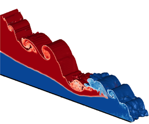
As a representative example, figure 5 shows the evolution of the two-layer gravity current for run 10, with  $R_{\rho }=2$ and $R_h=1$. Upon removal of the gate, the lower layer (in blue) develops a distinct head, whereas the upper layer (in red) forms a wedge-like intrusion behind the lower-layer head, cf. figure 5(a). The shear along the interface between the ambient and dense fluids results in the formation of strong Kelvin–Helmholtz vortices. As the current propagates further, we can distinguish a dense head of lower-layer fluid and a more dilute wake containing both upper and lower-layer fluid (figure 5b). These findings are similar to previous experimental observations (Gladstone et al. Reference Gladstone, Ritchie, Sparks and Woods2004; Dai Reference Dai2017; Wu & Dai Reference Wu and Dai2020; He et al. Reference He, Zhu, Zhao, Chen, Lin and Yuan2021). The wake region immediately behind the head is characterised by strong turbulent mixing of the lock fluid layers, whereas further back, the two dense layers remain more distinct, as seen in figure 5(c). The mixed region gradually expands, as dense fluid from the head is transported into the turbulent wake (figure 5d).

Figure 5. Instantaneous concentration isosurfaces  $c_U=0.1$ and $c_L=0.1$, along with the concentration field for both upper and lower layers for run 10 ( $R_{\rho }=2$ and $R_h=1$), (a) $t=5$, (b) $t=10$, (c) $t=15$ and (d) $t=20$.
Figure 6 compares three cases with identical thickness ratio  $R_h=1$, but different density ratios $R_{\rho }$, i.e. runs 2–4. For a moderate density ratio $R_{\rho }=1.25$, the fronts emerging from the upper and lower lock layers initially have comparable velocities, and significant mixing occurs near the head of the current (figure 6a). For larger density ratios ( $R_{\rho }=2$ and 4), on the other hand, the lower layer front propagates much faster than the upper layer front, so that the current head consists nearly entirely of lower-layer fluid, which was also observed by Wu & Dai (Reference Wu and Dai2020). The upper, red layer advances much more slowly, giving rise to much weaker Kelvin–Helmholtz vortices along its interface with the ambient fluid, along with much less-vigorous mixing (figure 6b,c).

Figure 6. Instantaneous concentration isosurfaces  $c_U=0.1$ and $c_L=0.1$, along with the concentration field for both upper and lower layers at $t=20$ for $R_h=1$: (a) run 2 for $R_{\rho }=1.25$, (b) run 3 for $R_{\rho }=2$ and (c) run 4 for $R_{\rho }=4$.
Figure 7 focuses on flows with constant density ratio  $R_{\rho }=4$ and different thickness ratios $R_h$, i.e. runs 1, 4, 7 and 14. For $R_h=0$, the lower layer is absent and the upper layer propagates as a single-layer gravity current (figure 7a). For the small but finite value $R_h=0.1$, the thin lower layer lubricates the much thicker upper layer, so that the upper layer advances faster than for $R_h=0$. Note that the head of the upper layer outruns the lower layer front (figure 7b). A similar trend was also observed by Gladstone et al. (Reference Gladstone, Ritchie, Sparks and Woods2004), Dai (Reference Dai2017), Wu & Dai (Reference Wu and Dai2020) and He et al. (Reference He, Zhu, Zhao, Chen, Lin and Yuan2021). The conditions under which this can occur are discussed in more detail in the following section. For $R_h=0.25$ the two front velocities are similar, and significant mixing occurs in the head region (figure 7c). For $R_h=1.5$, on the other hand, the lower layer front propagates faster than the upper layer, so that the current head consists mostly of lower-layer fluid (figure 7d). We now proceed to a more quantitative analysis of the dependence of the front velocity, energy budget, mixing and entrainment on $R_{\rho }$ and $R_h$.

Figure 7. Instantaneous concentration isosurfaces  $c_U=0.1$ and $c_L=0.1$, along with the concentration field for both upper and lower layers for $R_{\rho }=4$: (a) run 1 for $R_h=0$ at $t=30$, (b) run 4 for $R_h=0.1$ at $t=30$, (c) run 7 for $R_h=0.25$ at $t=30$ and (d) run 14 for $R_h=1.5$ at $t=18$.
3.2. Front velocity
We define the front positions  $X_{f,U}$ and $X_{f,L}$ of the upper and lower layers as the rightmost locations in the flow field with $c_U=0.5$ and $c_L=0.5$, respectively. This large threshold value is selected so that small amounts of fluid from one layer that have become entrained into the other layer do not result in a spurious front location value. The respective front velocities are then obtained as $U_{f,U} = {\rm {d}} X_{f,U} / {\rm {d}} t$ and $U_{f,L}={\rm {d}} X_{f,L}/{\rm {d}} t$.
Figure 8 displays the front velocities as functions of time for runs 4 and 10. For single-layer currents, it is well known that they proceed through a short acceleration phase into a constant-velocity slumping phase that can last for an extended period of time and typically extends over approximately four lock lengths (Rottman & Simpson Reference Rottman and Simpson1983). Figure 8 indicates that the two-layer gravity currents of the present study stay within the slumping phase throughout the entire simulation, as their front velocity, which is determined by the rate at which the more advanced layer propagates, remains approximately constant. The slower layer, on the other hand, displays a highly unsteady front velocity, as it is strongly affected by the turbulent wake of the current head.

Figure 8. Upper and lower layer front velocities  $U_f$ as a function of time for different density ratios $R_{\rho }$ and height ratios $R_h$. (a) The lower layer moves ahead of the upper layer for run 10 ( $R_{\rho }=2$, $R_h=1$). (b) The upper layer overtakes the lower layer for run 4 ( $R_{\rho }=4$, $R_h=0.1$).
Figure 8(a) shows that for run 10 the velocity of the lower, faster layer remains approximately constant, whereas that of the upper, slower layer fluctuates with time. Figure 8(b), on the other hand, indicates that for run 4 the upper, faster layer propagates at an approximately constant velocity, whereas the lower, slower layer decelerates and does not develop a quasi-steady front velocity.
We now proceed to employ the conservation of mass and vorticity to develop a circulation model for the case of a faster lower layer, by building on the earlier work by Borden & Meiburg (Reference Borden and Meiburg2013). Figure 9 presents the schematic flow field. After removal of the gate, the lower-layer lock fluid forms a right-propagating gravity current front of height  $h_{gc,L}$ with velocity $U_{f,L}$. Far behind the front, a discontinuity propagates with velocity $U_{r,L}$ to the left. Simultaneously, a counter current of velocity $U_0$ emerges in the ambient fluid above the gravity current. Subsequently, the upper-layer lock fluid also forms a gravity current of height $h_{gc,U}$ and velocity $U_{f,U}$ that propagates on top of the lower layer fluid. The flow is fully described by eight dimensionless unknowns: $U_{f,L}$, $U_0$, $U_{r,L}$, $U_{f,U}$, $U_U$, $U_{r,U}$, $h_{gc,L}$ and $h_{gc,U}$.

Figure 9. Model flow for predicting the upper and lower layer front velocities  $U_{f,U}$ and $U_{f,L}$.
Within control volume EFGI, and in the reference frame moving with the lower layer fluid, mass conservation for the ambient fluid gives
 \begin{equation} U_{f,L}h_{gc,L}=U_0(H-h_{gc,L}). \end{equation}
Because no vorticity enters the control volume, and vorticity flows out of the control volume confined to a thin vortex sheet between the lower layer and the ambient fluid, the vorticity flux is equal to the vortex sheet strength  $U_0+U_{f,L}$, multiplied by the sheet's principal velocity $(U_0+U_{f,L})/2$. The vorticity conservation at the interface gives
 \begin{equation} R_{\rho}h_{gc,L}=\tfrac{1}{2}(U_0+U_{f,L})^2. \end{equation}
In control volume DEIJ, in the reference frame moving with the upper layer, the mass conservation for the ambient fluid, along with vorticity conservation at the upper surface of the upper layer can be written as
 \begin{gather} U_0(H-h_{gc,L})+U_{f,U}h_{gc,U}=U_{r,U}(H-h_{gc,L}-h_{gc,U}), \end{gather}
 \begin{gather}h_{gc,U}=\tfrac{1}{2}(U_{r,U}+U_{f,U})^2. \end{gather}
For control volume CDJK, in the frame moving with the disturbance of the upper layer, mass and vorticity conservation yields
 \begin{gather} U_{r,U}(H-h_{gc,L}-h_{gc,U})=U_U(H-h_{gc,L})+U_{f,U}h_{gc,U}, \end{gather}
 \begin{gather}H-h_{gc,L}-h_{gc,U}=\tfrac{1}{2}(U_{f,U}+U_{r,U})^2. \end{gather}
Similarly in control volume BCKM, in the frame moving with the disturbance of the lower layer, mass and vorticity conservation leads to
 \begin{gather} U_U(H-h_{gc,L})=U_{r,L}(H-h_{gc,L}-h_U), \end{gather}
 \begin{gather}(R_{\rho}-1)(h_L-h^L_{gc})=(U_{f,L}+U_U)\left(\frac{U_{f,L}-U_U}{2}+U_{r,L}\right). \end{gather}
By combining these equations, we obtain for the dimensionless front velocity and height of the upper and lower layer gravity currents
 \begin{gather} U_{f,L}= \frac{(2+2R_h-h_{gc,L})\sqrt{2R_{\rho}h_{gc,L}}}{2(1+R_h)},\quad U_{f,U} = \frac{\sqrt{2h_{gc,U}}}{2}-\frac{h_{gc,L}\sqrt{2R_{\rho}h_{gc,L}}}{2(1+R_h)}. \end{gather}
 \begin{gather}h_{gc,L}=\frac{R_h(1+R_h)(3R_{\rho}-2)-R_h\sqrt{R_{\rho}(1+R_h)[R_{\rho}(9+R_h)-8]}}{R_h(2R_{\rho}-1)-1}, \end{gather}
 \begin{gather}h_{gc,U}=\frac{(1+R_h)(R_{\rho}R_h-2)+R_h\sqrt{R_{\rho}(1+R_h)[R_{\rho}(9+R_h)-8]}}{2R_h(2R_{\rho}-1)-2}. \end{gather}
 Figure 10 compares simulation results for the upper and lower layer front velocities with corresponding experimental data of He et al. (Reference He, Zhu, Zhao, Chen, Lin and Yuan2021), and with predictions by (3.9a,b). We observe generally good agreement, as reflected by the coefficient of determination  $R^2=0.814$. We note that for $R_h=0$, i.e. in the absence of a lower layer, (3.9a,b) yields the correct solution $U_{f,U}=\sqrt {2}/2$ for single-layer currents (Borden & Meiburg Reference Borden and Meiburg2013). In the limit of $R_\rho =1$, the two layers have identical density and form a single-layer current with $U_{f,U}=\sqrt {2(R_h+1)}/2$, which is again consistent with Borden & Meiburg (Reference Borden and Meiburg2013). If we mix the two lock layers initially so as to form a homogeneous lock fluid, a single-layer current forms with front velocity $\sqrt {2(1+R_hR_{\rho })}/2$, based on the circulation model and the half-depth assumption. Corresponding data, indicated in figure 10, suggest that the front velocity of a two-layer current is quantitatively similar to that of an equivalent, initially well-mixed single-layer current.

Figure 10. The black and blue symbols compare simulation results for the upper and lower layer front velocities, along with experimental data by He et al. (Reference He, Zhu, Zhao, Chen, Lin and Yuan2021), to corresponding predictions by (3.9a,b). The experimental data are for cases with  $R_{\rho }=5$ for $R_h=0.34$ and 0.13. For all cases the lower layer moves faster than the upper layer. Also shown by red symbols are the corresponding simulation results for single-layer currents and predictions by $\sqrt {2(1+R_hR_{\rho })}/2$.
Figure 11 shows predictions for the front velocities by (3.9a,b) as functions of  $R_h$, for different values of $R_{\rho }$. Here $U_{f,L}$ increases with $R_h$ and $R_{\rho }$. When $R_{\rho }$ is small, $U_{f,U}$ increases slightly for all $R_h$. For larger $R_{\rho }$, on the other hand, $U_{f,U}$ decreases for all $R_h$ values. This illustrates the competing effects of increased potential energy conversion and larger ambient counter-current velocity. We furthermore note that as $R_{\rho }$ increases, a smaller value of $R_h$ will suffice to ensure that the lower layer propagates faster than the upper layer.

Figure 11. Predictions by (3.9a,b) for the upper and lower layer front velocities,  $U_{f,U}$ and $U_{f,L}$, as functions of $R_h$, for different values of $R_{\rho }$.
3.3. Energy budget
The initial potential energy stored in the upper and lower dense fluid layers acts as the source that drives the flow. Once the gate opens, this potential energy is partially converted into kinetic energy, which is subsequently dissipated by the action of viscosity. In the following, we analyse these energy conversion processes quantitatively, along with the energy transfer between the different fluid layers. Towards this end, we define the potential energy  $E_p$, kinetic energy $E_k$ and dissipated energy $E_d$, respectively, as
 \begin{gather} E_p(t)=\int^W_0\int^{H}_0\int^L_0 (c_U+R_{\rho}c_L)(y-h_L)\,\mathrm{d}x\,\mathrm{d}y\,\mathrm{d}z, \end{gather}
 \begin{gather}E_k(t)=\int^W_0\int^{H}_0\int^L_0 \tfrac{1}{2}(u^2+v^2+w^2)\,\mathrm{d}x\,\mathrm{d}y\,\mathrm{d}z, \end{gather}
 \begin{gather}E_d(t)=\int^t_0\varepsilon(\tau)\,\mathrm{d}\tau, \end{gather}
where  $u$,
$u$,  $v$ and $w$ indicate the fluid velocity components in the $x$,
$x$,  $y$ and $z$ directions. Note that we focus on the potential energy relative to the situation with ambient fluid everywhere. We choose the initial top boundary of the lower dense layer $y=h_L$ as our reference level, so that the initial potential energy contained in the upper lock layer is constant for all cases. Here $\varepsilon$ indicates the instantaneous viscous dissipation rate
 \begin{equation} \varepsilon(t) = \int^W_0\int^{H}_0\int^L_0 \frac{2}{Re}s_{ij}s_{ij}\,\mathrm{d}x\,\mathrm{d}y\,\mathrm{d}z, \end{equation}
with  $s_{ij}$ denoting the rate-of-strain tensor
 \begin{equation} s_{ij} = \frac{1}{2}\left(\frac{\partial u_i}{\partial x_j}+\frac{\partial u_j}{\partial x_i}\right). \end{equation}
As the fluid is at rest initially, the overall energy budget of the flow takes the form
 \begin{equation} E_{total}=E_p+E_k+E_d=\mathrm{const.}=E_{p,init}, \end{equation}
where  $E_{p,init}$ represents the initial potential energy. To analyse the time-dependent conversion of potential, kinetic and dissipated energy, and the energy transfer among the different layers, we consider the respective contributions of the individual layers to the overall energy budget:
 \begin{gather} E_k=E_{kU}+E_{kL}+E_{k0}, \end{gather}
 \begin{gather}E_p=E_{pU}+E_{pL}, \end{gather}
 \begin{gather}E_d=E_{dU}+E_{dL}+E_{d0}, \end{gather}
 \begin{gather}\varepsilon=\varepsilon_U+\varepsilon_L+\varepsilon_0, \end{gather}
where the subscripts  $U$,
$U$,  $L$ and $0$ again refer to the upper layer, lower layer and ambient fluid, respectively. These contributions take the form
 \begin{gather} E_{kU}(t)=\int^W_0\int^{H}_0\int^L_0 c_U\tfrac{1}{2}(u^2+v^2+w^2)\,\mathrm{d}x\,\mathrm{d}y\,\mathrm{d}z, \end{gather}
 \begin{gather}E_{kL}(t)=\int^W_0\int^{H}_0\int^L_0 c_L\tfrac{1}{2}(u^2+v^2+w^2)\,\mathrm{d}x\,\mathrm{d}y\,\mathrm{d}z, \end{gather}
 \begin{gather}E_{k0}(t)=\int^W_0\int^{H}_0\int^L_0 (1-c_U-c_L)\tfrac{1}{2}(u^2+v^2+w^2)\,\mathrm{d}x\,\mathrm{d}y\,\mathrm{d}z, \end{gather}
 \begin{gather}E_{pU}(t)=\int^W_0\int^{H}_0\int^L_0c_U(y-h_L)\,\mathrm{d}x\,\mathrm{d}y\,\mathrm{d}z, \end{gather}
 \begin{gather}E_{pL}(t)=\int^W_0\int^{H}_0\int^L_0R_{\rho}c_L(y-h_L)\,\mathrm{d}x\,\mathrm{d}y\,\mathrm{d}z, \end{gather}
 \begin{gather}\varepsilon_U(t)=\int^W_0\int^{H}_0\int^L_0c_U\frac{2}{Re}s_{ij}s_{ij}\,\mathrm{d}x\,\mathrm{d}y\,\mathrm{d}z, \end{gather}
 \begin{gather}\varepsilon_L(t)=\int^W_0\int^{H}_0\int^L_0c_L\frac{2}{Re}s_{ij}s_{ij}\,\mathrm{d}x\,\mathrm{d}y\,\mathrm{d}z, \end{gather}
 \begin{gather}\varepsilon_0(t)=\int^W_0\int^{H}_0\int^L_0(1-c_U-c_L)\frac{2}{Re}s_{ij}s_{ij}\,\mathrm{d}x\,\mathrm{d}y\,\mathrm{d}z. \end{gather}
 Figure 12 shows the time evolution of all energy components for the representative example of run 9 with  $R_{\rho }=1.25$ and $R_h=1$. Note that all energy components are normalised by the initial potential energy of the upper dense layer $E_{pU,init}$. The total energy $E_{total}$ varies by around $1.5\,\%$ of $E_{pU,init}$ over the course of the simulation, which suggests that energy is conserved with good accuracy throughout the simulation.

Figure 12. Time history of the various energy budget components for run 9 with  $R_{\rho }=1.25$ and $R_h=1$.
For the first 10 time units the potential energy of the upper and lower dense layers rapidly decreases as the lock fluid collapses, whereas the kinetic energy of all three layers increases. Around  $t \approx 10$, the collapse of the lower layer is nearly complete and its potential energy levels off. For late times, its potential energy even increases slightly due to mixing processes that tend to lift up parcels of dense fluid. On the other hand, the upper dense fluid layer continues to lose potential energy. The kinetic energy of all three layers levels off after $t \approx 10$. For late times $E_{kU}$ and $E_{kL}$ gradually decrease due to the effects of dissipation. The dissipated energy grows slowly with time for all three layers.
Figure 13 shows the influence of the density ratio  $R_{\rho }$ and the height ratio $R_h$ on the evolution of the different energy components. Figure 13(a) indicates that the kinetic energy and dissipation of the upper layer do not vary significantly with the lower layer density, even though the upper layer loses potential energy faster in the presence of a denser lower layer that collapses more quickly. Figure 13(b) shows that the energetics of the lower layer are affected more strongly by an increase in $R_{\rho }$. As the density of the lower layer increases, it converts potential energy into kinetic energy more quickly, and it dissipates energy at a faster rate. As a larger height ratio $R_h$ also causes the lower layer to propagate faster, $R_h$ has a similar influence on the lower layer energy components as $R_{\rho }$, cf. figure 13(d). On the other hand, the dynamics of the upper layer are affected more strongly by $R_h$ than by $R_{\rho }$, cf. figure 13(c). Here $E_{kU}$ and $E_{dU}$ increase with $R_h$, because for larger $R_h$, the upper layer can descend to a lower vertical level, which enables it to convert more potential energy into kinetic energy.

Figure 13. The evolution of the various energy budget components for different  $R_{\rho }$ and $R_h$: (a) upper layer energy components for $R_h=1$ and different $R_{\rho }$ values, i.e. runs 9–11; (b) lower layer energy components for $R_h=1$ and different $R_{\rho }$ values; (c) upper layer energy components for $R_{\rho }=1.25$ and different $R_h$, i.e. runs 5, 9 and 12; and (d) lower layer energy components for $R_{\rho }=1.25$ and different $R_h$.
For a single-layer gravity current, the dense fluid always transfers energy to the ambient fluid, e.g. Necker et al. (Reference Necker, Härtel, Kleiser and Meiburg2002) and He et al. (Reference He, Zhao, Hu, Yu and Lin2018). For a two-layer gravity current the situation becomes more complex, as shown in figure 14. In this figure we analyse the change in total energy for each individual fluid layer,  ${\rm \Delta} E_U$, ${\rm \Delta} E_L$ and ${\rm \Delta} E_0$, in order to obtain insight into the energy transfer between the different layers. Although the ambient fluid gains energy for all values of $R_{\rho }$ and $R_h$, and the upper dense layer always loses energy, the lower dense layer can gain or lose energy, depending on the specific values of the governing dimensionless parameters. This net energy gain of the lower dense layer, as a result of energy transfer from the upper layer, is perhaps somewhat unexpected. To quantify this effect as function of $R_\rho$ and $R_h$, we focus on the normalised ${\rm \Delta} E_U$ and ${\rm \Delta} E_L$ at the representative time $t=20$. Figure 15(a) presents ${\rm \Delta} E_U$ as a function of $R_h$ for different values of $R_\rho$. We find that to a good approximation ${\rm \Delta} E_U$ varies linearly with $R_h$. Thus, we look for a scaling parameter of the form $R^{\lambda _1}_{\rho } R_h$. Figure 15(b) shows that the raw data are well fitted ( $R^2=0.997$) by a straight line of the form
 \begin{equation} \frac{{\rm \Delta} E_U}{E_{pU,init}}={-}0.2-1.1R^{0.2}_{\rho}R_h. \end{equation}
The intersect with the vertical axis at  $-$0.2 indicates that the upper layer loses about $20\,\%$ of its initial energy when $R_h=0$. This suggests that a single-layer gravity current with a small aspect ratio will transfer approximately $20\,\%$ of its initial energy to the ambient fluid, as the lock fluid collapses and forms the gravity current. A similar conclusion can also be found from Zhu, He & Meiburg (Reference Zhu, He and Meiburg2021). On the other hand, the energy variation of the upper layer mainly comes from the decrease of the potential energy $E_{pU}$, which is shown in figure 13. $E_{pU}$ changes approximately linearly with $R_h$. However, a larger $R_\rho$ results in a faster lower layer, which enhances the loss of $E_{pU}$ indirectly. Equation (3.30) captures the linear and nonlinear dependence of $E_{pU}$ on $R_h$ and $R_\rho$, respectively, and it reflects that the decrease of $E_U$ depends more strongly on $R_h$ than on $R_\rho$.

Figure 14. Time history of the variation of the total energy of the upper layer fluid  ${\rm \Delta} E_U$, the lower layer fluid ${\rm \Delta} E_L$ and the ambient fluid ${\rm \Delta} E_0$ for the cases with (a) $R_h=1$ and different $R_{\rho }$, i.e. runs 9–11, and (b) $R_{\rho }=1.25$ and different $R_h$, i.e. runs 5, 9 and 12.

Figure 15. Variation of the total energy of the upper layer fluid  ${\rm \Delta} E_U$, and of the lower layer fluid ${\rm \Delta} E_L$, for different values of $R_{\rho }$ and $R_h$.
Figure 15(c) shows the normalised  ${\rm \Delta} E_L$ as a function of the height ratio $R_h$ for different density ratios $R_\rho$. As $R_h$ increases, ${\rm \Delta} E_L$ initially increases as well, but it subsequently reaches a maximum and then decreases. This suggests that for small $R_h$ the lower layer gains more energy from the upper layer than it transfers to the ambient fluid, whereas for large $R_h$ this situation is reversed. We find that the raw data depend parabolically on $R^{0.8}_{\rho } R_h$, as seen in figure 15(d). A good fit ( $R^2=0.999$) is achieved by
 \begin{equation} \frac{{\rm \Delta} E_L}{E_{pU,init}}={-}0.1(R^{0.8}_{\rho} R_h-1)^2+0.1. \end{equation}
When  $R_h=0$, the lower layer does not exist and ${\rm \Delta} E_L$ is zero. Equation (3.31) also indicates that the lower layer gains a maximum of $10\,\%$ of the initial upper layer energy, when $R^{0.8}_{\rho } R_h=1$. Here $R^{0.8}_{\rho } R_h$ can be roughly interpreted as representing the mass of the lower layer. A lower layer of larger mass obtains more energy from the upper layer, up to a threshold beyond which the effect of the upper layer on the lower layer starts to wane, and the lower layer transfers more energy to the ambient fluid.
3.4. Mixing of the upper and lower layers
We now proceed to analyse and quantify the mixing dynamics between the upper and lower dense fluid layers, which strongly affects the overall propagation rate of the two-layer current. In order to obtain insight into the Lagrangian mixing behaviour, we mark individual fluid patches by passive tracers of different colours, so that we can easily track them throughout the evolution of the flow, cf. figure 16. Depending on whether the lower dense layer advances faster or more slowly than the upper layer, we observe different mixing patterns.

Figure 16. Temporal evolution of Lagrangian mixing between upper and lower layer fluids. (a) Run 9 ( $R_{\rho }=1.25$, $R_h=1$): the lower layer fluid propagates faster and forms the head of the current. Significant mixing occurs in the wake of the head. (b) Run 2 ( $R_{\rho }=1.25$, $R_h=0.1$): the upper layer fluid propagates faster and forms the current head. Relatively little mixing occurs between upper and lower layer fluids.
When the lower layer propagates faster, it rapidly forms a head after the gate is removed. The fluid in the head is carried upward by the ambient counterflow, so that it mixes with both the upper dense layer and the ambient fluid through the action of the interfacial Kelvin–Helmholtz vortices. The fluid within the head is constantly being replenished by the near-wall layer of the current, which moves faster than the head itself. It also entrains upper-layer fluid in a wedge-like shape behind the head, so that the entire head region becomes vigorously mixed, as shown in figure 16(a).
When the upper dense layer advances more rapidly than the lower layer, it surges ahead of the lower layer and forms the head of the current, cf. figure 16(b). Very little lower layer fluid enters the head under these conditions, and the two layers mix much less than in the flow of figure 16(a).
Previous studies have shown that the interfacial instabilities in stratified flow can help to predict the mixing properties between different layers (Balasubramanian & Zhong Reference Balasubramanian and Zhong2018; Martin, Negretti & Hopfinger Reference Martin, Negretti and Hopfinger2019). Holmboe (Reference Holmboe1962) predicted Kelvin–Helmholtz instability and Holmboe instability at small and large Richardson numbers, respectively. The bulk Richardson number  $J=g'\delta /({\rm \Delta} U)^2$ is defined, whereas Kelvin–Helmholtz instabilities can only occur when $J<0.07$. Here, $g'$ is the reduced gravity, $\delta ={\rm \Delta} U/(\partial U/\partial y)_{max}$ is the shear layer thickness and ${\rm \Delta} U$ is the velocity difference between the two layers or the current and the ambient fluid. Hazel (Reference Hazel1972) found that Holmboe instabilities exist when $\delta /\eta >2$, where $\eta ={\rm \Delta} \rho /(\partial \rho /\partial y)_{max}$ is the density layer thickness, and ${\rm \Delta} \rho$ is the density difference. We have measured $J$ and $\delta /\eta$ from several profiles in different cases, which are presented in table 3.
Table 3. Parameters  $J$ and $\delta /\eta$ for different cases.

Table 3 shows that the bulk Richardson numbers at the interface of the upper or lower layer and ambient fluid  $J_{U0}$ or $J_{L0}$ are less than 0.07 for all cases. Kelvin–Helmholtz instability is observed, as shown in figures 6 and 7. Note that for run 6, the upper and lower layers have similar front velocity, so a clear interface of the lower layer and ambient fluid does not exist. However, for the interface of the upper and lower layers, the bulk Richardson number $J_{UL}$ is always larger than 0.07. In most of the cases $\delta _{UL}/\eta _{UL}$ is higher than 2, so that Holmboe instability occurs. In run 11, the large density ratio decreases the shear layer thickness, resulting in a small value of $\delta _{UL}/\eta _{UL}$, which suppresses the Holmboe instability.
In order to quantify the mixing of upper and lower layer fluids as a function of  $R_{\rho }$ and $R_h$, we follow a computational approach similar to that of Tokyay, Constantinescu & Meiburg (Reference Tokyay, Constantinescu and Meiburg2011), and evaluate the normalised volume $V_m$ within which the concentrations of the upper and lower layer fluids both exceed a threshold value $c_t$:
 \begin{gather} V_m=\frac{1}{L_s\times h_U\times W}\int^H_0\int^L_0 \int^W_0\gamma_{UL}\,\mathrm{d}x\,\mathrm{d}y\,\mathrm{d}z, \end{gather}
 \begin{gather}\gamma_{UL}=\left\{\begin{array}{@{}ll} 1 & c_U>c_t\ {\rm and}\ c_L>c_t,\\ 0 & {\rm otherwise.} \end{array}\right. \end{gather}
Figure 17 shows the temporal evolution of  $V_m$ for different values of $R_{\rho }$, $R_h$ and $c_t=0.02$. It demonstrates that $R_{\rho }$ has a non-monotonic influence on the time history of $V_m$, so that at least during some flow stages mixing is most pronounced for intermediate values of $R_{\rho }$. These complex dynamics result from the competing effects of density stratification: on the one hand, strong stratification tends to suppress mixing; on the other hand, it increases the velocity difference between the layers, and thereby enhances the interfacial shear, which tends to promote mixing. At the same time, a larger velocity difference between the layers results in a head region that contains very little upper layer fluid, which in turn reduces mixing.

Figure 17. Time development of the mixed volume  $V_m$ for the height ratio $R_h=1$ with different density ratios $R_{\rho }$ (i.e. runs 9–11); and for the density ratio $R_{\rho }=1.25$ with different height ratios $R_h$ (i.e. runs 2, 5 and 9).
Figure 17 also indicates that a larger height ratio  $R_h$ uniformly tends to promote mixing, as it allows the dense fluid layers to release more potential energy, and to generate a more vigorous flow.
Similar to our approach in § 3.3, we evaluate the mixed volume  $V_m$ at $t=20$ for different cases to show the quantitative dependence on the density ratio $R_{\rho }$ and height ratio $R_h$. Figure 18(a) presents $V_m$ as a function of $R_h$ for different $R_{\rho }$. Here $V_m$ increases with $R_h$, but is significantly reduced for large values of $R_{\rho }$. Figure 18(b) shows that for $R^{-0.25}_{\rho } R^{0.5}_h$ as the scaling parameter, the raw data can be well fitted ( $R^2=0.962$) by a straight line of the form
 \begin{equation} V_m=1.3R^{{-}0.25}_{\rho} R^{0.5}_h. \end{equation}
This equation is consistent with the fact that for  $R_h=0$ no mixed fluid is being generated. Although a larger $R_h$ results in more mixing, an increase in $R_{\rho }$ reduces the mixed volume $V_m$.

Figure 18. The mixed volume  $V_m$ for different $R_{\rho }$ and $R_h$.
As the approach of Tokyay et al. (Reference Tokyay, Constantinescu and Meiburg2011) is affected by the concentration threshold, we also present and compare the results of two alternate approaches for quantifying the mixing of the upper and lower layers. The first is based on the framework of Winters et al. (Reference Winters, Lombard, Riley and D'Asaro1995). In the closed system of our configuration, the increase in the background potential energy  $E_b$ results only from mixing, so that the evolution of $E_b$ is a direct measure of the mixing. The background potential energy $E_b$ is defined as
 \begin{equation} E_b = \int^W_0\int^{H}_0\int^L_0 (c_U+R_Lc_L)(y_*-h_L)\,\mathrm{d}x\,\mathrm{d}y\,\mathrm{d}z, \end{equation}
where  $y_*$ is the vertical position in the state of the minimum potential energy. Note that here we also choose the initial top boundary of the lower dense layer $y = h_L$ as our reference level.
Figure 19 shows the time history of the normalised background potential energy  $(E_b-E_{b,init})/E_{pU,init}$ for different cases. Here $E_{b,init}$ is the initial background potential energy. The energy $E_b$ increases with time, which implies the presence of the irreversible mixing. However, different from the conclusion presented by figure 17, $E_b$ monotonically increases with the density ratio $R_{\rho }$. This may be due to the fact that the density of the lower layer directly affects the calculation of the background potential energy. On the other hand, the evolution of $E_b$ quantitatively presents the mixing not only between the upper and lower layers but also between the two layers and ambient fluid.

Figure 19. Time history of the normalised background potential energy  $(E_b-E_{b,init})/E_{pU,init}$ for the height ratio $R_h=1$ with different density ratios $R_{\rho }$ (i.e. runs 9–11); and for the density ratio $R_{\rho }=1.25$ with different height ratios $R_h$ (i.e. runs 2, 5 and 9).
As a second approach, we first calculate the volumes that the upper layer, lower layer and the two-layer current occupy (García Reference García1993). They are defined as  $V_U$, $V_L$ and $V_{UL}$:
 \begin{gather} V_U=\frac{\left(\displaystyle\int^W_0\int^{H}_0 \int^L_0 c_U\,\mathrm{d}x\,\mathrm{d}y\,\mathrm{d}z\right)^2}{\displaystyle\int^W_0\int^{H}_0 \int^L_0 c_U^2\,\mathrm{d}x\,\mathrm{d}y\,\mathrm{d}z}, \end{gather}
 \begin{gather}V_L=\frac{\left(\displaystyle\int^W_0\int^{H}_0\int^L_0 c_L\,\mathrm{d}x\,\mathrm{d}y\,\mathrm{d}z\right)^2}{\displaystyle\int^W_0\int^{H}_0 \int^L_0 c_L^2\,\mathrm{d}x\,\mathrm{d}y\,\mathrm{d}z}, \end{gather}
 \begin{gather}V_{UL}=\frac{\left(\displaystyle\int^W_0\int^{H}_0\int^L_0 c_U+c_L\,\mathrm{d}x\,\mathrm{d}\,y\mathrm{d}z\right)^2}{\displaystyle\int^W_0\int^{H}_0\int^L_0 (c_U+c_L)^2\,\mathrm{d}x\,\mathrm{d}y\,\mathrm{d}z}. \end{gather}
Then, the normalised mixed volume  $V_{m,G}$ can be obtained as
 \begin{equation} V_{m,G} = \frac{V_U+V_L-V_{UL}}{L_s\times h_U\times W} .\end{equation}
 Figure 20 shows the time history of the normalised mixed volume  $V_{m,G}$ for different cases. The values of $V_{m,G}$ are smaller than $V_m$ shown in figure 17, which indicates that this method has a larger concentration threshold to define the boundary of the currents. At the same time, $V_{m,G}$ exhibits a monotonic decrease with the increase of the density ratio $R_\rho$. However, the values of $V_m$ show the strongest mixing occurs for intermediate $R_\rho$, as larger values of $R_\rho$ cause more low-concentration mixing.

Figure 20. Time evolution of the normalised mixed volume  $V_{m,G}$ for the height ratio $R_h=1$ with different density ratios $R_{\rho }$ (i.e. runs 9–11); and for the density ratio $R_{\rho }=1.25$ with different height ratios $R_h$ (i.e. runs 2, 5 and 9).
3.5. Entrainment in two-layer gravity currents
As an essential feature, propagating gravity currents entrain ambient fluid, thus increasing their volume. The entrainment dynamics of two-layer currents are more complex than for single-layer currents, because they involve the interfaces of both layers with the ambient fluid. Following Ottolenghi et al. (Reference Ottolenghi, Adduce, Inghilesi, Armenio and Roman2016), we define the entrainment velocity as the volume flux per unit area of the ambient fluid across the interface with the gravity currents:
 \begin{equation} U_e(t)=\frac{Q(t)}{0.5[S(t)+S(t-{\rm \Delta} t)]}. \end{equation}
Here  $S(t)=W d_e(t)$ denotes the interfacial area at time $t$, where we define $d_e(t)$ as the rightmost location in the flow field with $c_U=0.02$ or $c_L=0.02$. Before the ambient counter-current reaches the left wall, $d_e(t)$ is the distance between this location and the front of the left-propagating ambient counter-current. Here $Q(t)$ is the instantaneous volume flux across the interface:
 \begin{equation} Q(t)=\frac{V(t)-V(t-{\rm \Delta} t)}{{\rm \Delta} t}, \end{equation}
where the volume of the two-layer gravity current is obtained as
 \begin{gather} V(t)=\int^W_0\int^H_0\int^L_0\gamma\,\mathrm{d}x\,\mathrm{d}y\,\mathrm{d}z, \end{gather}
 \begin{gather}\gamma=\left\{\begin{array}{@{}ll} 1 & {c_U>c_t\ \mathrm{or}\ c_L>c_t,}\\ 0 & \mathrm{otherwise.} \end{array}\right. \end{gather}
As a threshold value we take  $c_t=0.02$, consistent with Ottolenghi et al. (Reference Ottolenghi, Adduce, Inghilesi, Armenio and Roman2016). The instantaneous entrainment parameter $E(t)$ of the current is then obtained as the ratio of the entrainment velocity to the front velocity of the two-layer gravity current relative to the ambient fluid:
 \begin{equation} E(t)=\frac{U_e(t)}{2U_f(t)}. \end{equation}
Here, we assume that the ambient fluid flows to the left with approximately  $U_f(t)$, so that the velocity difference between the current and the ambient is $2U_f(t)$. The time-averaged entrainment behaviour of the flow is characterised by the bulk parameters:
 $$\begin{gather} \bar{Q}(t)=\frac{V(t)-V(0)}{t}, \end{gather}$$
 $$\begin{gather}\bar{U}_e(t)=\frac{\bar{Q}(t)}{0.5[S(t)+S(0)]}, \end{gather}$$
 $$\begin{gather}\bar{U}_f(t)=\frac{X_f(t)-X_f(0)}{t}, \end{gather}$$
 $$\begin{gather}\bar{E}(t)=\frac{\bar{U}_e(t)}{2\bar{U}_f(t)}. \end{gather}$$
 Figure 21 compares the entrainment dynamics of single- (run 8 for  $R_{\rho }=1$ and $R_h=1$) and two-layer (run 10 for $R_{\rho }=2$ and $R_h=1$) gravity currents. Figure 21(a,b) show the bulk and instantaneous entrainment fluxes, $\bar {Q}$ and $Q$. Early on the dense fluid collapses and forms a well-defined head. Kelvin–Helmholtz billows evolve along the upper boundary and entrain ambient fluid, so that the bulk entrainment flux $\bar {Q}$ increases with time. After the ambient counter-current reaches the left wall of the tank at $t \approx 12$, $\bar {Q}$ levels off, with a larger value for the two-layer case. As compared with the bulk entrainment flux, the instantaneous flux $Q$ exhibits more complex behaviour characterised by pronounced peaks. To establish the reasons for these peaks, we turn to the streamwise vorticity field averaged over the spanwise direction, cf. figure 22. Consistent with earlier work by Ottolenghi et al. (Reference Ottolenghi, Adduce, Inghilesi, Armenio and Roman2016), we find that the Kelvin–Helmholtz billows trap the most ambient fluid when they reach their maximum size and intensity, resulting in the formation of instantaneous peaks in $Q$, cf. figure 22(a–d). The billows increase their size before the peak occurs, and they break down after that. Although the instantaneous fluxes $Q$ evolve qualitatively similarly for the single- and two-layer cases, $Q$ reaches a higher peak value for the two-layer case, cf. figure 22(e,f).

Figure 21. The time evolution of bulk and instantaneous entrainment properties for single- (run 8 for  $R_{\rho }=1$ and $R_h=1$, blue lines, right column) and two-layer (run 10 for $R_{\rho }=2$ and $R_h=1$, black lines, left column) gravity currents: (a,b) bulk and instant entrainment fluxes $\bar {Q}$ and $Q$; (c,d) bulk and instantaneous entrainment velocities $\bar {U}_e$ and $U_e$; (e,f) bulk and instantaneous entrainment parameters $\bar {E}$ and $E$.
$E$.

Figure 22. The dimensionless vorticity fields  $\omega _{xy}$ of single- (run 8 for $R_{\rho }=1$ and $R_h=1$) and two-layer (run 10 for $R_{\rho }=2$ and $R_h=1$) gravity currents: (a,c,e) for the two-layer case; (b,d,f) for the single-layer case.
Figure 21(c,d) show the time evolution of the bulk and instantaneous entrainment velocities,  $\bar {U}_e$ and $U_e$. The high early values are related to the initial collapse and the formation of the head (He et al. Reference He, Zhao, Hu, Yu and Lin2018). After $t \approx 12$, $\bar {U}_e$ and $U_e$ decrease, because the tail region of the currents does not give rise to significant entrainment (Bhaganagar Reference Bhaganagar2017). This is also reflected in the time evolution of the bulk and instantaneous entrainment parameters, $\bar {E}$ and $E$, cf. figure 21(e,f). For both single- and two-layer flows we observe $\bar {E}$ and $E$ of $O(10^{-2})$, which is consistent with earlier investigations (Ottolenghi et al. Reference Ottolenghi, Adduce, Inghilesi, Armenio and Roman2016; He et al. Reference He, Zhao, Hu, Yu and Lin2018, Reference He, Zhao, Zhu and Hu2019).
Figure 23 shows the influence of the density ratio  $R_{\rho }$ and the height ratio $R_h$ on the evolution of the bulk entrainment parameter $\bar {E}$ for two-layer gravity currents. Figure 23(a) demonstrates that $\bar {E}$ decreases for larger $R_{\rho }$, since stronger stratification tends to dampen the Kelvin–Helmholtz instability while causing a larger front velocity. The effects of the layer height ratio $R_h$ are analysed in figure 23(b). Until the left-propagating counter-current encounters the left wall, $R_h$ has only a minor influence on $\bar {E}$, because the entrainment is dominated by the lower-layer current. After the reflection of the counter-current from the left wall, however, it is evident that larger $R_h$-values enhance entrainment, so that $\bar {E}$ increases.

Figure 23. The evolution of bulk entrainment parameter  $\bar {E}$ for two-layer gravity currents as a function of front location $X_f$ with different $R_{\rho }$ and $R_h$: (a) $R_h=1$ with different $R_{\rho }$, i.e. runs 9–11; (b) $R_{\rho }=1.25$ with different $R_h$, i.e. runs 5, 9 and 12.
3.6. Constant excess weight
As mentioned in § 2.1, so far we have employed the thickness and density of the upper layer to scale the simulations. Consequently, the total excess weight in the initial condition has not been held constant for the different cases. In this section, we keep the total excess weight constant and run several cases with different density and height ratios of the upper and lower layers.
We introduce characteristic length and velocity scales  $\hat {H}/2$ and $\hat {u}_{b,A}= \sqrt {\hat {g}\hat {H}(\hat {\rho }_A-\hat {\rho }_0)/2\hat {\rho }_0}$ to non-dimensionalise the governing equations. Here $\hat {\rho }_A=(\hat {\rho }_U \hat {h}_U+\hat {\rho }_L \hat {h}_L)/\hat {H}$ is the average density of the lock fluid. The non-dimensional (2.10)–(2.12) can be rewritten as
 \begin{gather} \frac{\partial u_i}{\partial t}+u_j\frac{\partial u_i}{\partial x_j}={-}\frac{\partial p}{\partial x_i}+\frac{1}{Re_A} \frac{\partial^2 u_i}{\partial x_j\partial x_j}+(R_Uc_U+R_Lc_L)\,{\rm e}^{g}_i, \end{gather}
 \begin{gather}\frac{\partial c_U}{\partial t}+u_j\frac{\partial c_U}{\partial x_j}= \frac{1}{Pe}_A\frac{\partial^2 c_U}{\partial x_j\partial x_j}, \end{gather}
 \begin{gather}\frac{\partial c_L}{\partial t}+u_j\frac{\partial c_L}{\partial x_j}=\frac{1}{Pe}_A\frac{\partial^2 c_L}{\partial x_j\partial x_j}. \end{gather}
The dimensionless parameters are the Reynolds number  ${Re}_A$,
 \begin{equation} {Re}_A=\frac{\hat{u}_{b,A}\hat{H}}{2\hat{\nu}}, \end{equation}
the Péclet number  ${Pe}_A$,
 \begin{equation} {Pe}_A=\frac{\hat{u}_{b,A}\hat{H}}{2\hat{\kappa}}, \end{equation}
and the density parameters for the upper layer  $R_U$ and lower layer $R_L$,
 \begin{gather} R_U=\frac{\hat{\rho}_U-\hat{\rho}_0}{\hat{\rho}_A-\hat{\rho}_0}, \end{gather}
 \begin{gather}R_L=\frac{\hat{\rho}_L-\hat{\rho}_0}{\hat{\rho}_A-\hat{\rho}_0}. \end{gather}
The initial and boundary conditions are as described in § 2.2. The parameters of the simulations are listed in table 4. All cases have the same averaged density of the two-layer lock fluids.
Table 4. Simulation cases and parameters.

Figure 24 shows the evolution of the two-layer gravity currents with different density ratio  $R_{\rho }$ and height ratio $R_h$. Although having different stratification, the two-layer currents propagate at comparable velocities, due to the identical initial averaged density $\rho _A$. Figure 24(a–c) compare three cases with constant height ratio $R_h=1$ but different density ratio $R_{\rho }$, i.e. runs 15–17. With increasing $R_{\rho }$, the upper layer slows down and the main body of the currents becomes thinner. Figure 24(d–f) present the flows with identical density ratio $R_{\rho }=1.5$ and different height ratio, i.e. runs 16, 18 and 19. When increasing $R_h$, the lower layer has a larger volume but smaller density. For a small height ratio $R_h=0.25$, the fronts of the upper and lower layers have similar velocities. For larger height ratios ( $R_h=1$ and 4), the lower layer propagates faster than the upper layer.

Figure 24. Instantaneous concentration field, along with the concentration isosurfaces  $c_U=0.5$ and $c_L=0.5$ for both upper and lower layers at $t=30$: (a–c) runs 15–17 for $R_h=1$ and $R_{\rho }=1$, 1.5 and 3; (d–f) runs 18, 16 and 19 for $R_{\rho }=1.5$ and $R_h=0.25$, 1 and 4.
4. Conclusions
We have employed three-dimensional direct numerical simulations to investigate the mixing and entrainment dynamics, as well as the energetics, of gravity currents emerging from a two-layer stratified lock. The dominant governing dimensionless parameters take the form of a layer thickness ratio  $R_h$ and a density ratio $R_{\rho }$. Depending on the values of these parameters, the simulations show that either the upper layer or lower layer fluid can propagate faster, so that it forms the head of the overall gravity current. Similarly, the simulations clarify the role of $R_h$ and $R_{\rho }$ in determining the long-term density structure of the gravity current, which can range from strongly stratified to near-complete mixing. These simulation results outline possible scenarios for the behaviour of certain classes of turbidity currents and powder snow avalanches, with a dense, concentrated layer near the base and a more dilute layer above. In particular, the simulations demonstrate that depending on the specific flow conditions, either the dense or the dilute layer can propagate more rapidly.
Building on the earlier circulation-based approach introduced by Borden & Meiburg (Reference Borden and Meiburg2013), we propose a theoretical model for predicting the overall gravity current height, along with the front velocity of the two layers, when the lower layer moves faster than the upper layer. This model clarifies the role of the height and thickness ratios in determining the velocity structure of the current, and it sheds light on the dynamics of the ambient counter-current as it slows down the propagation of the upper gravity current layer.
By conducting a detailed analysis of the energy budget, we have been able to quantify the conversion between potential and kinetic energy as a function of the parameters  $R_{\rho }$ and $R_h$. This analysis also clarifies the energy transfer rates between the different layers of the gravity current, and from the gravity current to the ambient fluid. In particular, it shows that the dense gravity current layer may gain or lose energy, depending on the specific flow conditions.
Further work is needed in order to clarify how the present results may change in the presence of a sloping bottom, or how they may be modified if the scalar field has a settling velocity associated with it, if it exchanges mass with the bed through erosion or deposition, or if it gives rise to non-Newtonian rheology.
Funding
Funding for this work was provided under NSF grant CBET-2138583, under the National Natural Science Foundation of China (52171276), as well as by the Key Research and Development Program of Zhejiang Province (2021C03180). Computational resources for this work used the Extreme Science and Engineering Discovery Environment (XSEDE), supported by the National Science Foundation, USA, grant no. TG-CTS150053. R.Z. thanks the China Scholarship Council for providing him with a scholarship to study at UCSB.
Declaration of interests
The authors report no conflict of interest.


 Open access