


1. Introduction
Gas flows in nature and engineering applications are quite often turbulent and, in certain cases, may carry a dispersed solid or liquid particulate phase. This configuration imposes additional complexities on the analysis of the field, as the kinematics of the particles are coupled to the magnitude and distribution of the carrier-phase turbulent energy. The response of the flow's turbulent properties to the presence of suspended particulates is known as turbulence modulation. The modulation problem has been thoroughly analysed utilizing both experimental and numerical approaches. Considering the number of parameters which characterize two-phase flows (Gore & Crowe Reference Gore and Crowe1991) and, as a result, impact modulation, it is not surprising that investigations continue unabated. Liquid droplets, however, have received far less scrutiny than their solid (usually spherical) counterparts. Setting aside the obvious discrepancy in deformation capabilities, liquid droplets often evaporate at a rate that is highly dependent on the level of gaseous turbulence, thus adding another layer of complication to the modulation problem. Furthermore, the issue of droplet vaporization lies at the heart of spray combustion systems which power the world's transportation needs.
Broadly speaking, modulation investigations either analyse the global properties of a heavily laden flow or focus on the near-interface fluid dynamics of a small number of particles. The former represents a more realistic test case and helped build a foundation of knowledge on the subject. The latter has become more feasible with advances in computing power and full-field experimental techniques such as particle image velocimetry (PIV). Gore & Crowe (Reference Gore and Crowe1989) summarized much of the early experimental work on particle-laden jet and pipe flows and suggested that the ratio of particle diameter to integral length scale,  $d/L$, provides a strong indication of whether the (centreline) turbulent energy is increased (augmentation) or decreased (attenuation). The kinetic energy of small particles ( $d/L \lesssim 0.1$) is increased through drag at the expense of the carrier phase turbulent kinetic energy (TKE), $k$, whereas large particles ( $d/L \gtrsim 0.1$) tend to promote wakes which, in turn, increase the level of turbulence in the flow. In another review published in the same year and incorporating the same data, Hetsroni (Reference Hetsroni1989) favoured a particle Reynolds number, $Re_p$, of ${\sim }400$ as the demarcation between attenuation and augmentation, where the wakes (specifically, vortex shedding) presumed to exist at elevated $Re_p$ are again given credit for increasing the turbulence level. Hetsroni (Reference Hetsroni1989) also addressed the lack of reliable experimental data. Around that time, the first direct numerical simulation (DNS) investigations appeared (Squires & Eaton Reference Squires and Eaton1990; Elghobashi & Truesdell Reference Elghobashi and Truesdell1993). These studies, and many that would follow, utilized a point-particle approach, where the fluid–particle interaction is modelled. Although the point-particle strategy is approximately restricted to sub-Kolmogorov particles, even today it remains the economical choice for simulating practical atomization processes at realistic Reynolds numbers. Both aforementioned DNS studies analysed the turbulent dissipation rate, $\varepsilon$, a quantity that traditionally defied reliable experimental calculation, and both concluded that the sub-Kolmogorov particles extract energy from the large scales and transfer it to the small scales, ultimately increasing the dissipation rate. To avoid digressing into a very complex topic, we now focus on the research with the most relevant attributes to the present work: experimental campaigns in homogeneous and isotropic turbulence (HIT), analyses of fixed particles and studies focused on near-particle kinetic energy and dissipation.
Poelma & Ooms (Reference Poelma and Ooms2006) surveyed the existing literature pertaining to the effect of a particulate phase on the turbulent characteristics of HIT. They cited only three experimental studies (Schreck & Kleis Reference Schreck and Kleis1993; Hussainov et al. Reference Hussainov, Kartushinsky, Rudi, Shcheglov, Kohnen and Sommerfeld2000; Geiss et al. Reference Geiss, Dreizler, Stojanovic, Chrigui, Sadiki and Janicka2004) that emphasized carrier-phase modification – each used grid-generated turbulence and single-point laser diagnostics. Schreck & Kleis (Reference Schreck and Kleis1993) reported a significant increase in the downstream decay rate of TKE with the addition of a modest concentration ( $\phi < 0.015$, where $\phi$ is the volume fraction) of buoyant plastic and heavy glass particles to a turbulent water flow. Plots of unladen spectra indicated anisotropy at the large and small scales, and the addition of particles helped improve the overlap of the longitudinal and lateral spectral curves at high wavenumbers (small-scale isotropy). Hussainov et al. (Reference Hussainov, Kartushinsky, Rudi, Shcheglov, Kohnen and Sommerfeld2000) used air as the carrier phase instead of water and presented clear attenuation of the turbulent energy by large glass particles. Interestingly, Geiss et al. (Reference Geiss, Dreizler, Stojanovic, Chrigui, Sadiki and Janicka2004) reported significant augmentation of the carrier-phase TKE when an airflow was laden with $480\,\mathrm {\mu }{\rm m}$ glass beads at ${\phi = 0.004}$. In contrast to Schreck & Kleis (Reference Schreck and Kleis1993), they reported particle-induced anisotropy. Downstream particle-induced anisotropy was confirmed by Poelma, Westerweel & Ooms (Reference Poelma, Westerweel and Ooms2007) in water tunnel grid turbulence. The anisotropy is caused by a transfer of turbulent energy from the cross-stream to the streamwise component, and the effect increases with mass loading. Unsatisfied with the existing strategies (or lack thereof) to correlate the modulation effect, Poelma et al. (Reference Poelma, Westerweel and Ooms2007) suggested that the particle-induced dissipation increases linearly with the product of the Stokes number, $S_k$, and a non-dimensional number density. They also showed a major slip-induced wake structure by ensemble averaging the near-particle PIV fields. The redistribution of energy from large to small scales is clearly depicted in spectral plots – a phenomenon termed ‘pivoting’. Finally, Poelma et al. (Reference Poelma, Westerweel and Ooms2007) demonstrated that the particle production of turbulence, by virtue of remaining relatively constant, can become non-negligible when compared with the total turbulent dissipation, which decays along the flow direction. Practical applications notwithstanding, the significant mean flow inherent in grid turbulence makes elucidating the effects of the pure turbulent fluctuations a challenge.
When experimentalists aim to analyse a problem in the absence of bulk convection, they typically turn to zero-mean-flow (ZMF) chambers. Many studies in this area (Fallon & Rogers Reference Fallon and Rogers2002; Yang & Shy Reference Yang and Shy2003; Good et al. Reference Good, Ireland, Bewley, Bodenschatz, Collins and Warhaft2014) focused on the particle dynamics, including clustering phenomena and the settling velocity, but as diagnostic techniques and experimental objectives evolved, it became possible to extract additional information from the fluid. Yang & Shy (Reference Yang and Shy2005) quite clearly illustrated a directional dependence on the attenuation vs augmentation regimes of falling spheres – an effect which becomes more dramatic with increasing  $S_k$. Augmentation of the spectra generally begins around the Taylor microscale. Hwang & Eaton (Reference Hwang and Eaton2006) dropped small, heavy spheres ( $S_k \sim 50$) through a chamber with eight synthetic jet actuators and, surprisingly, noted a global decrease in dissipation rate. This contradicts the spectral pivoting theory but, it should be noted, is not the only study that finds $\varepsilon$ attenuated (Boivin, Simonin & Squires Reference Boivin, Simonin and Squires1998). When comparing the results from various studies, it is not entirely clear if the near-surface dissipation is always treated in a consistent manner – for instance, after a plot showing a major decrease in $\varepsilon$ with increasing mass loading, Hwang & Eaton (Reference Hwang and Eaton2006) introduced a new and separate dissipation term, $\varepsilon _p$, which designates the extra dissipation due to particles. A recent study by Petersen, Baker & Coletti (Reference Petersen, Baker and Coletti2019) used a large jet-stirred tank to produce zero-mean turbulence and confirmed the pivoting effect described by Poelma et al. (Reference Poelma, Westerweel and Ooms2007). The high levels of anisotropy, however, were not recreated. Petersen et al. (Reference Petersen, Baker and Coletti2019) speculated that the large Reynolds number in their study contributed to the more evenly distributed energy.
The two ZMF experimental studies that are most relevant to the present campaign are Tanaka & Eaton (Reference Tanaka and Eaton2010) and Hoque et al. (Reference Hoque, Mitra, Sathe, Joshi and Evans2016). Tanaka & Eaton (Reference Tanaka and Eaton2010) took the familiar configuration of mono-disperse spheres falling through a jet-stirred chamber and added sub-Kolmogorov-resolution two-dimensional (2-D)-PIV ( $\Delta x/\eta = 0.55$, where $\Delta x$ is the vector spacing and $\eta$ is the Kolmogorov scale). This opened up the potential to resolve the dissipation using spatial gradients, and they presented the ensemble near-particle dissipation and kinetic energy fields for $500\,\mathrm {\mu }{\rm m}$ spheres of glass along with $250\,\mathrm {\mu }{\rm m}$ spheres of glass and polystyrene. Tanaka & Eaton (Reference Tanaka and Eaton2010) reported strong attenuation of $k$ out to $r/R \approx 2$, where $r/R$ is the radial coordinate normalized by the droplet radius, and surface dissipation rates up to three times larger than the unladen value, $\varepsilon _0$. The falling particles promote asymmetries in the $k$ and $\varepsilon$ fields in most cases, complicating the interpretation. Hoque et al. (Reference Hoque, Mitra, Sathe, Joshi and Evans2016) implemented yet another common test rig – water agitated between two oscillating grids – added a fixed glass sphere of variable diameter ( $10 \lesssim d/\eta \lesssim 77$), and analysed the field via 2-D-PIV. Unlike Tanaka & Eaton (Reference Tanaka and Eaton2010), Hoque et al. (Reference Hoque, Mitra, Sathe, Joshi and Evans2016) did not achieve sub-Kolmogorov resolution, yet the study is unique since it is perhaps the only experimental investigation in HIT that holds the object fixed in place. Despite the PIV resolution, spatial gradients were used to calculate $\varepsilon$, and the expected near-surface increase was verified. The TKE was generally augmented because of the large size of the spheres ( $d/L \geq 0.32$). Neither study developed data in the $d/\eta < 1$ regime.
To truly capture the near-interface dynamics, the configuration must be particle (or interface) resolved. Numerically, a particle-resolved strategy implies that the near-particle mesh is fine enough to properly resolve the flow gradients introduced by the no-slip boundary condition – the extent of the grid cells is typically many times smaller than the unladen Kolmogorov length scale,  $\eta _0$. No interface modelling/approximations are required if a spherical, body-fitted mesh is employed; the no-slip and kinematic constraints existing at the interface are introduced as boundary conditions on the relevant cell faces. To mitigate the computational expense of body-fitted spherical grids centred at each particle, alternative approaches including the immersed boundary and lattice Boltzmann methods are commonly applied to high-volume-fraction flows. The most relevant numerical studies are particle-resolved DNS (PR-DNS) with one or more fixed spheres. The authors of these studies generally acknowledge the limited scope of the fixed-in-place configuration but extol the benefits of first understanding the simplified physics surrounding spheres that cannot convert fluid turbulence into their own kinetic energy. The studied configurations include turbulent channel flow (Zeng et al. Reference Zeng, Balachandar, Fischer and Najjar2008; Mehrabadi et al. Reference Mehrabadi, Tenneti, Garg and Subramaniam2015; Peng, Ayala & Wang Reference Peng, Ayala and Wang2020), decaying HIT (Bagchi & Balachandar Reference Bagchi and Balachandar2004; Burton & Eaton Reference Burton and Eaton2005; Botto & Prosperetti Reference Botto and Prosperetti2012) and stationary HIT (Vreman Reference Vreman2016). The Vreman (Reference Vreman2016) simulation of 64 fixed spheres ( $d/\eta = 2$) arranged in a cubic lattice (separation of $8d$,
$8d$,  $\phi = 0.001$) and exposed to a stationary HIT field ( $Re_\lambda = 32$) with no mean flow is conditionally closest to the present experiments. The radially averaged $k$ field returns to 93 % of the unladen value, with 90 % recovery achieved at approximately $r/R = 5$. More importantly, the surface dissipation spikes to over $100\varepsilon _0$. We hope to recreate these types of informative radial profiles using experimental data.
The term ‘particle resolved’ is rarely associated with experiments; we suggest an experiment may be reasonably classified as particle resolved if it provides full-field velocity information, starting at the fluid–particle interface and extending outward to several normalized radii, with sub-Kolmogorov resolution. Such a definition does not feel overly restrictive (especially when broad comparisons with DNS studies are desired) and yet, to the best of our knowledge (the introductory statement in Vreman (Reference Vreman2016) concurs), there is but a single experiment that falls into this category – the aforementioned Tanaka & Eaton (Reference Tanaka and Eaton2010) study. While sub-Kolmogorov resolution is a prerequisite to determining  $\varepsilon$ via the spatial gradient method (Tanaka & Eaton Reference Tanaka and Eaton2007, Reference Tanaka and Eaton2010; Verwey & Birouk Reference Verwey and Birouk2022), experiments can still provide valuable insight into single-point statistics such as $k$. Even so, relaxing the sub-Kolmogorov resolution requirement does not introduce many additional experimental studies. Experiments and simulations with poor near-particle resolution may also be inadequate for global modulation predictions; Vreman (Reference Vreman2016) found that over 10 % of the total dissipation occurs in 0.5 % of the flow volume. The region of extreme dissipation is made up of the shells surrounding the particles where, as previously mentioned, surface dissipation values can exceed the corresponding unladen quantities by a factor of 100.
While the volume of literature pertaining to modulation in general is extensive, only a small fraction examined the effects of droplet evaporation. Early DNS studies (Mashayek Reference Mashayek1998; Miller & Bellan Reference Miller and Bellan1999; Wang & Rutland Reference Wang and Rutland2006) indicated that liquid drops help return kinetic energy to the flow as they evaporate. This effect may not be noticed depending on the initial conditions pertaining to liquid–vapour equilibrium (Russo et al. Reference Russo, Kuerten, van der Geld and Geurts2014). More recent DNS investigations have utilized a particle-resolved strategy, but evaporative feedback on the carrier turbulence was either not the focus (Dodd et al. Reference Dodd, Mohaddes, Ferrante and Ihme2021), too weak to have any effect (Lupo et al. Reference Lupo, Gruber, Brandt and Duwig2020) or negligible compared with the liquid-phase modulation (Shao, Jin & Luo Reference Shao, Jin and Luo2022). Experimental studies are seemingly non-existent (Elghobashi Reference Elghobashi2019).
1.1. Summary and objectives
The default fundamental turbulent flow is one that is homogeneous and isotropic with a negligible mean component. It is, therefore, interesting that very little benchmark experimental data have been collected in this regime for the complex problem of particle/droplet modulation. To provide straightforward validation cases and general insight, we analysed with 2-D-PIV the modulation induced by a single suspended water droplet in both sub- and super-Kolmogorov regimes, primarily in the  $Re_\lambda$ range of 50–140. The fixed droplet geometry reduced the (extensive) parameters at play and allowed us to focus on the relative size effect – this configuration is also relevant for heavy particles which do not react kinematically to the flow (Burton & Eaton Reference Burton and Eaton2005) and, at the other end of the spectrum, small drops which are travelling with the mean. The latter possibility is often mentioned in conjunction with dilute fuel sprays, hence rapidly evaporating ethanol droplets were also investigated. Results are intuitively presented in physical space in the form of spatial heat maps and radially averaged profiles. Furthermore, the experimental details and processing techniques are allocated additional space due to the infrequent publication of similar campaigns.
2. Experimental methods
2.1. Overview
Four parameters were independently manipulated in this study: the droplet diameter, the droplet composition (non-volatile vs volatile), the TKE of the carrier phase and the composition of the carrier phase. Variation of the droplet diameter was achieved by controlling the initial diameter,  $d_0$, and by continuously monitoring the flow field via PIV as the drop evaporated. The droplet was either water or ethanol – the former approximated a non-volatile case, while ethanol introduced the effects of rapid mass transfer and surface regression. Turbulence was generated via eight fans which agitated the gas in an enclosed chamber – the level of turbulent kinetic energy was altered by adjusting the rotational speed, $N$, at which the fans were driven, where $k^{1/2} \propto N$. The study primarily utilized helium as the background gas. Due to the high kinematic viscosity of helium, it was possible to resolve the Kolmogorov scales with standard PIV equipment (Verwey & Birouk Reference Verwey and Birouk2022). Furthermore, the relatively large size of $\eta$ in helium allowed the inclusion of the important $d/\eta < 1$ flow regime. Selected test points were repeated in nitrogen, and although the dissipation of nitrogen could not be calculated directly, comparisons of TKE modulation made it a valuable addition. Room temperature and atmospheric pressure were maintained throughout the study.
2.2. Fan-stirred spherical chamber
Experiments were performed in a  $0.029\,{\rm m}^3$ fan-stirred spherical chamber. Eight fans, each having six blades and a diameter of 100 mm, direct flow toward the centre of the chamber to create a stationary HIT field. Although 2-D-PIV and droplet suspension studies have been performed extensively in the chamber, this was the first attempt to merge the two techniques. The fans were operated up to 5465 RPM and were checked with a stroboscope before and after each set of tests, ensuring that no fan deviated from the nominal target speed by more than 0.5 %. The helium or nitrogen environment was created by first evacuating the sealed chamber with a vacuum pump and then adding the desired gas from a commercial cylinder. The most comprehensive summary of the chamber characteristics may be found in Verwey (Reference Verwey2022). Key details are presented in figure 1.

Figure 1. (a) Overhead and (b) cross-sectional view (camera perspective) of the spherical chamber. The light sheet blockage is depicted in (b) for a droplet of exaggerated diameter. The red square in (b) is the camera FOV, approximately to scale.
Droplets were suspended at the intersection of two  $14\,\mathrm {\mu }{\rm m}$ silicon carbide fibres with a retractable injector. The fibres were mounted in a spring-tensioned frame that placed their intersection at the geometric centre of the chamber. The fibre orientation – typically consisting of a vertical and horizontal fibre crossing at $90^{\circ }$ – was switched to an ‘X’ pattern such that the vertical laser sheet struck only the droplet hanging at the intersection. A small node of epoxy ( ${\sim }180\,\mathrm {\mu }{\rm m}$ in diameter) was placed at the fibre intersection to increase the maximum supported droplet diameter.
2.3. Particle image velocimetry
The PIV system consists of a Litron Nano L 135-15 Nd:YAG dual-head laser synchronized to a 12-bit,  $2048 \times 2048\,{\rm px}$ camera with a pixel pitch, $d_r$, of $7.4\,\mathrm {\mu }{\rm m}$ and a repetition rate of 10 Hz. A 60 mm lens was coupled with a 3 $\times$ teleconverter and provided a magnification, $M$, of 0.65 and a field of view (FOV) of $23 \times 23$ mm. The pulse separation, $\Delta t$, was set by first examining the particle displacement probability density functions of sample cases and determining the value of $\Delta t$ that ensured 99 % of particle displacements would be less than $\Delta X/4$ (the ‘one-quarter’ rule), where $\Delta X$ is the interrogation area (IA) width. The alignment and calibration were carefully achieved using symmetrical features of the chamber and a professionally machined calibration target. The true magnification of any imaged tracer particle was estimated to be within 1 % of the global value. Before acquiring images, the flow was densely seeded with olive oil tracers/drops that were primarily atomized in the sub-micron range. A tracer particle of $1\,\mathrm {\mu }{\rm m}$ diameter had a maximum Stokes number of ${\sim }0.01$, where $S_k < 0.1$ is the typical criterion for assuming negligible tracer slip (Tropea, Yarin & Foss Reference Tropea, Yarin and Foss2007). DynamicStudio software was used to cross-correlate the images using $32 \times 32\,{\rm px}$ IAs ( $\Delta X = 364\,\mathrm {\mu }{\rm m}$) with 50 % overlap ( $\Delta x = 182\,\mathrm {\mu }{\rm m}$). All other processing and analysis tasks were performed using in-house MATLAB scripts.
2.3.1. Preliminary considerations
The goal of this study was to determine how an isotropic turbulent flow reacts to the introduction of a small liquid droplet at a spatially fixed location. We were primarily concerned with the modification of turbulence statistics – in particular,  $k$ and $\varepsilon$ – close to the droplet surface. To retrieve this information via 2-D-PIV, the droplet must be located within the laser sheet. This configuration yielded two experimental problems: reflections that obscured tracer particle imaging in the interface region and the blockage of laser light on one side of the droplet. The greater context of this experiment – namely, the interaction between turbulence and droplet vaporization – meant that interface characterization was critical. Fortunately, liquid droplets can be dyed with a fluorophore to mitigate reflectivity issues. The fluorophoric powder rhodamine B is readily soluble in many common liquids, including water and ethanol. Data collected by Kristoffersen et al. (Reference Kristoffersen, Erga, Hamre and Frette2014) indicated absorption peaks at 554 and 550 nm in water and ethanol solvents, respectively. Approximately 80 % of incoming 532 nm radiation (typical for frequency-doubled Nd:YAG lasers, including the one used presently) will be absorbed and re-emitted in a relatively narrow band surrounding the peak emission wavelengths of 576 and 569 nm for water and ethanol, respectively. This fluorescence was filtered out by a 532 nm laser line filter – a standard optical component often used by default in a PIV experiment to reduce stray light impingement (e.g. ambient room lighting) on the camera sensor. Deionized water mixed with rhodamine B at a concentration of $1\,{\rm g}\,{\rm l}^{-1}$ was used for the non-volatile investigation. Ethanol mixed with trace amounts of rhodamine B was implemented for the volatile case.
The second issue – that of laser sheet blockage – resulted in a rectangular region on one side of the droplet being devoid of illuminated tracer particles. The spherical symmetry of both flow field and obstruction (the droplet itself) made the resultant data loss relatively unimpactful, as statistics are theoretically independent of azimuthal and polar angles. Furthermore, the sharp cutoff in image intensity imposed by the blockage was used to solve another problem – calculating the droplet diameter. Suspended droplets are typically imaged using high-magnification optics illuminated with a backlight. The sequence of silhouettes is readily analysed using standard image processing techniques such as thresholding and opening, and the diameter extracted by counting the remaining object pixels,  $N_p$, and assuming sphericity if reasonable, where
 \begin{equation} d = \frac{d_r}{M}\sqrt{\frac{4}{\rm \pi}N_p}. \end{equation}
However, diameter information cannot be obtained in this manner concurrently with PIV – a complimentary strategy was devised. If the ratio of droplet diameter to laser sheet thickness,  $d/\Delta z_0$, is large enough, the extent of the blockage region should conform almost perfectly to $d$. The utility of this strategy is verified in the following section.
2.3.2. Feasibility investigation
The general capability of correlating blockage region to object size was evaluated by inserting needles of known diameter (300, 462, 902 and  $1273\,\mathrm {\mu }{\rm m}$, each measured with a micrometer to within ${\pm }3\,\mathrm {\mu }{\rm m}$) perpendicular to the laser sheet. A steep transition from high to low average row intensity occurred near the edges of the blockage region. The needles were used to determine the weight, $w$, such that the number of rows falling below the cutoff intensity, $I_{{cut}}$, was equal to the true object size, where
 \begin{equation} I_{{cut}} = \min(\overline{I_{{row}}}) + w\left(\overline{I_{{rec}}} - \min(\overline{I_{{row}}})\right). \end{equation}
In (2.2),  $\overline {I_{row}}$ is the row-averaged image intensity and $\overline {I_{rec}}$ is the overall area-averaged intensity in the near-droplet region – both are limited in calculation to the right-hand side of the droplet where the blockage region exists. Consider the example calibration image in figure 2(a). A $300\,\mathrm {\mu }{\rm m}$ needle – its presence visible as a bright white dot at $(x, y) \approx (0, 0)$ mm – blocks the laser sheet. With a pixel pitch of $7.4\,\mathrm {\mu }{\rm m}$ and a magnification of 0.65, each pixel represents $11.38\,\mathrm {\mu }{\rm m}$ in the object plane. Hence, a height of 26 pixels most closely approximates the needle diameter. The value of $w$ in (2.2) is incremented – beginning at zero and in steps of 0.01 – until 26 rows have average intensity values less than $I_{{cut}}$. For the example provided in figure 2, the best weight was 0.26 and the resultant (normalized) cutoff intensity is depicted by the blue dashed line in figure 2(b). The results were averaged over 100 images which, in the case of the $300\,\mathrm {\mu }{\rm m}$ needle, yielded an average optimal weight, $w_o$, of 0.30. Fortunately, the average optimal weight was rather insensitive to seeding density – $w_o$ did not change by more than 0.01 when comparing minimally ( ${\sim }0.005$ particles per pixel) and maximally ( ${\sim } 0.02$ particles per pixel) seeded fields. When sizing droplets, (2.2) was used to establish $I_{{cut}}$ by letting $w = w_0 = 0.30$ for all images.

Figure 2. (a) A PIV calibration image with the  $300\,\mathrm {\mu }{\rm m}$ needle inserted perpendicular to the laser sheet. The average row intensities $\overline {I_{row}}$ are calculated within the green bordered area. These averages are normalized by the overall region intensity $\overline {I_{rec}}$ (the region demarcated with the light green overlay) and plotted in (b). The normalized cutoff intensity for this image is depicted by the blue dashed line; 26 rows have intensities less than this cutoff value, as discussed above.
2.3.3. Set-up and calibration for droplets
For a typical PIV experiment in the spherical chamber, where all three velocity components feature nearly equivalent distributions,  $\Delta z_0$ could be set equal to $\Delta X$ and, provided $\Delta t$ is chosen using the strategy outlined in § 2.3, the one-quarter rule would be simultaneously satisfied for in- and out-of-plane tracer displacement as desired (Adrian & Westerweel Reference Adrian and Westerweel2011). The uniqueness of the present experiment, where complete obstruction of the light is requisite for sizing assessment, dictated that the sheet should be as thin as possible to accommodate smaller drops. The achievable light sheet thickness varies inversely with stand-off distance, where the minimum stand-off distance of 270 mm corresponds to a theoretical sheet thickness of ${\sim }260\,\mathrm {\mu }{\rm m}$ as measured by the $\mathrm {e}^{-2}$ criterion. The beam waist was placed at the fibre intersection by adjusting the manual focusing module, recording 200 images with a relatively high $\Delta t$, and observing which column of vectors featured the most substitutions (excessive substitutions being the result of out-of-plane pair loss, an effect which should be most dramatic at the beam waist). The optimal $\Delta t$ value was re-assessed based on $\Delta z_0 = 260\,\mathrm {\mu }{\rm m}$, which was smaller than $\Delta X$ ( $364\,\mathrm {\mu }{\rm m}$) and, therefore, drove the selection of $\Delta t$.
A spherical droplet does not present an identical blockage profile as compared with the cylindrical needles used for calibration. Even droplets satisfying  $d > \Delta z_0$ will allow ‘leakage’ of the laser light around the upper and lower periphery, since droplets present a circular, rather than rectangular, frontal area. A $182\,\mathrm {\mu }{\rm m}$ droplet blocks only 55 % of the light intercepted by a $182\,\mathrm {\mu }{\rm m}$ cylinder (assuming $\Delta z_0 = 260\,\mathrm {\mu }{\rm m}$, discussed above). However, at $d = 364\,\mathrm {\mu }{\rm m}$, this ratio has increased to over 90 %. This analysis is purely geometric and does not consider that the majority of leaked light belongs to the weaker-intensity tail regions of the sheet profile. The example diameters of 182 and $364\,\mathrm {\mu }{\rm m}$ were not picked at random; rather, they represent the edges of the smallest diameter bin, to be discussed shortly. It is reasonable to expect greater diameter uncertainty for such small droplets. We note, however, that this uncertainty is only capable of underpredicting the diameter. While a droplet reported as $182\,\mathrm {\mu }{\rm m}$ is quite likely to be larger, its placement in the $182\unicode{x2013}346\,\mathrm {\mu }{\rm m}$ bin remains justified.
2.3.4. Data processing and analysis
Whereas most modulation studies utilize particles of specific size, droplets of water and ethanol evaporate and, therefore, produce a continuous range of diameters. The droplet diameter at the end of a PIV run may be much smaller than  $d_0$, depending on the liquid and turbulence level. To facilitate statistical convergence, droplet images were binned based on diameter. Seven bins of $182\,\mathrm {\mu }{\rm m}$ width covered the diameter range of $182\unicode{x2013}1456\,\mathrm {\mu }{\rm m}$. The selection of bin width was somewhat arbitrary; however, $182\,\mathrm {\mu }{\rm m}$ corresponds to the vector spacing of the PIV grid and in a sense represents the minimum resolvable resolution. In doing so, we suggest that a group of droplets with diameters differing by not more than $182\,\mathrm {\mu }{\rm m}$ may be reasonably allocated to the same ensemble. The convergence criteria discussed below confirmed this assumption. Each diameter range is denoted by its mean value, $\bar {d}$, for notational convenience (e.g. the $182\unicode{x2013}364\,\mathrm {\mu }{\rm m}$ bin is equivalent to $\bar {d} = 273\,\mathrm {\mu }{\rm m}$). When discussing results, a particular case is typically identified by the ratio of the mean diameter to the unladen Kolmogorov scale, ${\bar {d}/\eta _0}$.
The PIV system is limited to  ${\sim }3000$ image pairs per acquisition cycle. The need for statistical convergence across seven diameter bins, combined with the above limitation, resulted in the repetition of each condition (where the term ‘condition’ defines the unique combination of liquid, TKE, and background gas) at least seven times. In the case of volatile ethanol at elevated TKE, the condition was repeated up to 50 times due to the rapid evaporation of the droplet. Each PIV test contains a continuous range of diameters beginning at $d_0$ and ending at either $d \leq 182\,\mathrm {\mu }{\rm m}$ or some intermediate diameter value that is reached when 3000 pairs have been acquired. Once the images were saved, they were transferred to MATLAB for analysis. The in-house code extracted the droplet diameter through the intensity weighting strategy discussed in previous sections. The midpoint between the cut off rows defined the droplet centroid in the $y$ direction, $y_c$. The laser flash was used to locate the front of the droplet which, since the diameter is known, leads to the $x$ centroid value, $x_c$. In the case of very small droplets, the flash was large compared with the droplet itself, which biased the droplet placement towards the left. In these instances, the value of $x_c$ was set to zero, which was justified since the fibre intersection corresponds to $(x,y) \approx (0,0)$, and also because small droplets did not move significantly with the flow field. Pixels at radial locations satisfying $r \leq d/2$, where $r = 0$ corresponds to ( $x_c,y_c$), were considered part of the droplet while pixels to the right of the droplet were considered part of the blockage region. The MATLAB script applied masks to the droplet and blockage regions of both frames, removed any large reflections (the front of the drop or the fibre intersection) by comparing the size of connected regions with the average tracer particle size, and returned the masked images to DynamicStudio. A raw and masked image example is presented in figure 3. The processed images were then cross-correlated in the typical fashion using the standard $32 \times 32\,{\rm px}$ interrogation areas with 50 % overlap. A second MATLAB script compiled an index of the location and file names for the vector and mask data that fell into each size bin. The final main processing step involved reading the vector data files randomly – along with the diameter and centroid information – and building an independent ensemble for each bin size. The information was selected at random to avoid biasing the results toward any particular PIV test. This process was continued until both the TKE and dissipation rates converged.

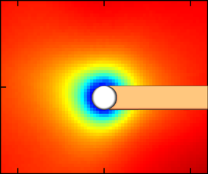
Figure 3. (a) Example of a (cropped) raw PIV image and (b) the masked sample ready for cross-correlation. The droplet diameter and centroid are extracted during the masking operation so that the resultant velocity vector field can be properly binned. In this example, the blockage region height is 123 px, or  $1400\,\mathrm {\mu }{\rm m}$. Hence, this droplet/vector field would be placed in the $1274\unicode{x2013}1456\,\mathrm {\mu }{\rm m}$ (or $\bar {d} = 1365\,\mathrm {\mu }{\rm m}$) bin associated with the given experimental condition.
To better accommodate the geometry of the experiment, the fluctuating Cartesian velocities,  $u$ and $v$, are transformed to a spherical basis, $u_r$ and $u_\phi$
 \begin{gather} u_r = \frac{u(x-\overline{x_c}) + v(y-\overline{y_c})}{((x - \overline{x_c})^2 + (y-\overline{y_c})^2)^{1/2}}, \end{gather}
 \begin{gather} u_\phi = \frac{-u(y-\overline{y_c}) + v(x-\overline{x_c})}{((x-\overline{x_c})^2 + (y-\overline{y_c})^2)^{1/2}}, \end{gather}
where  $(x,y)$ refers to the fixed PIV coordinate system and $(\overline {x_c}, \overline {y_c})$ is the mean centroid of the droplet ensemble (the construction of the droplet ensemble, including convergence considerations, is discussed shortly). To calculate the TKE, we assumed that the azimuthal and polar Reynolds shear stresses are equivalent
 \begin{equation} k = \frac{1}{2}\langle u_ru_r + u_\phi u_\phi + u_\theta u_\theta \rangle \approx \frac{1}{2}\langle u_r u_r \rangle + \langle u_\phi u_\phi \rangle, \end{equation}
where angled brackets signify a temporal average.
To calculate the dissipation rate from 2-D data, HIT approximations must be applied. Three formulations utilized by Hoque et al. (Reference Hoque, Mitra, Sathe, Joshi and Evans2016), Tanaka & Eaton (Reference Tanaka and Eaton2010) and Verwey & Birouk (Reference Verwey and Birouk2022) are provided in (2.6)–(2.8), respectively,
 \begin{gather} \varepsilon =3\nu\left\langle \frac{2}{3}\left(\frac{\partial u}{\partial x}\right)^2 + \left(\frac{\partial v}{\partial x}\right)^2 + \left(\frac{\partial u}{\partial y}\right)^2 + \frac{2}{3}\left(\frac{\partial v}{\partial y}\right)^2 + \frac{2}{3}\left(\frac{\partial u}{\partial y}\frac{\partial v}{\partial x}\right)\right\rangle, \end{gather}
 \begin{gather} \varepsilon =3\nu\left\langle \left(\frac{\partial u}{\partial x}\right)^2 + \left(\frac{\partial v}{\partial x}\right)^2 + \left(\frac{\partial u}{\partial y}\right)^2 + \left(\frac{\partial v}{\partial y}\right)^2 + 2\left(\frac{\partial u}{\partial y}\frac{\partial v}{\partial x}\right)\right\rangle, \end{gather}
 \begin{gather} \varepsilon =3\nu\left\langle \frac{5}{6}\left(\frac{\partial u}{\partial x}\right)^2 + \frac{7}{12}\left(\frac{\partial v}{\partial x}\right)^2 + \frac{7}{12}\left(\frac{\partial u}{\partial y}\right)^2 + \frac{5}{6}\left(\frac{\partial v}{\partial y}\right)^2 - \frac{\partial u}{\partial x}\frac{\partial v}{\partial y} - \frac{\partial v}{\partial x}\frac{\partial u}{\partial y}\right\rangle. \end{gather}
As they must, all three equations return identical results when the isotropic relations governing mean-square relationships hold perfectly, but their application to a real experimental dataset will inevitably lead to disagreements. In PIV measurements of single-phase HIT, with proper resolution and applying the correction suggested by Tanaka & Eaton (Reference Tanaka and Eaton2007), the deviation is small. For instance, in Verwey & Birouk (Reference Verwey and Birouk2022) the average per cent difference in  $\varepsilon$ values returned by (2.6) vs (2.8) across 42 independent tests was 0.6 %. However, the flow near the droplet interface is far from isotropic, even in the small-scale sense, which means the form of the dissipation equation will have a significant impact on the value of $\varepsilon$. Regardless of isotropy, the true dissipation field surrounding a fixed, spherical droplet in a zero-mean HIT field should be a function of only the radial coordinate. By this logic, the three methods may be contrasted based on the angular variation of dissipation by evaluating the normalized standard deviation of $\varepsilon$ in a thin region surrounding the droplet. Unfortunately (or perhaps fortunately), there was not enough discrepancy between methods to definitively select one over the other on that basis. That $\varepsilon$ varies only modestly with $\phi$ is confirmed by looking at the spatial heat maps of dissipation (§ 3.2.2) and suggests that the errors induced by assuming isotropy are mitigated to some extent. Nevertheless, the approximate nature of the near-interface dissipation values reported in this study must be acknowledged. Since the Tanaka & Eaton (Reference Tanaka and Eaton2010) study is the only modulation experiment that utilized PIV with sub-Kolmogorov resolution to resolve the near-particle $k$ and $\varepsilon$ fields, we elected to use their formula for $\varepsilon$, (2.7). Their study, while different from the present one in many ways, shares enough similarities to facilitate direct comparisons in the data – such comparisons will be most accurate if the dissipation formula is consistent. Of the three formulas, (2.7) returns the largest $\varepsilon$ values near the droplet. Finally, since all dissipation fields – including the unladen ones – were calculated using a consistent formula, it is hoped that dissipation data are insightful in a relative sense, even if their closeness to the true value is questionable.
To recover the dissipation rate in the interface vicinity, the spatial gradients in (2.7) were universally calculated using forward (in the radial sense) difference schemes instead of central differences. The flow field was divided into four quadrants with the origin at the droplet centroid. Gradients in the upper-right quadrant were forward in  $x$ and $y$, gradients in the upper-left quadrant were backward in $x$ and forward in $y$, etc. The forward differences were calculated for two different grid spacings, $2\Delta x$ and $3\Delta x$. These distinct spacings were necessary to implement the correction developed by Tanaka & Eaton (Reference Tanaka and Eaton2010),
 \begin{equation} \varepsilon^{(p,q)} \approx \frac{9\varepsilon_m^{(p,q)}|_{3\Delta x} - 4\varepsilon_m^{(p,q)}|_{2\Delta x}}{5}, \end{equation}
where  $(p,q)$ is the PIV grid index and $\varepsilon _m$ is the raw measured dissipation rate from (2.7). Equation (2.9) is a weighted average derived to suppress the extreme noise that prevails in sub-Kolmogorov-resolution PIV and propagates into the dissipation calculation. The individual mean-square gradients which comprise the dissipation rate can also be corrected in this manner.
The primary data analysis outputs are  $k$ and $\varepsilon$ averaged in thin radial shells, designated ${\overline {k_{\Delta r}}}$ and ${\overline {\varepsilon _{\Delta r}}}$, respectively. The shells begin at the ensemble droplet surface and extend out to the bounds of the field of view. Shell thickness, $\Delta r$, was set equal to $\Delta x$, or $182\,\mathrm {\mu }{\rm m}$. A shell-averaged statistic at radius $r$ incorporates all data between $(r-\Delta r/2)$ and $(r+\Delta r/2)$ – in other words, $r$ is the radial coordinate of the shell centreline. The convergence criteria were based on how these radial shell averages change as additional vector fields were added to the ensemble. In any given image, a pixel can belong to the droplet, the blockage region or the unobstructed background. Pixel associations are constantly changing due to evaporation (longer term effect) and drag-induced droplet motion, the latter of which can significantly affect the drop position even in sequential image pairs. The ensemble droplet representation was built by adding up the droplet masks from the individual image pairs and subsequently removing outliers. Pixel locations associated with the droplet at a rate of 20 % or less were rejected as outliers for the purpose of calculating the overall ensemble droplet radius, $R$, and centroid $(\overline {x_c},\overline {y_c})$. Ensemble statistics were updated after every 100 images. After each ensemble calculation, the newest values of ${\overline {k_{\Delta r}}}$ and ${\overline {\varepsilon _{\Delta r}}}$ were compared with the previous ones. Convergence was achieved once the deviation in both statistics – and in every shell – was less than 0.02 for five consecutive calculations. An example of the convergence of ${\overline {k_{\Delta r}}}$ and ${\overline {\varepsilon _{\Delta r}}}$ is illustrated in figure 4.

Figure 4. Illustration of convergence in radial shells for (a) the TKE and (b) the dissipation rate. Statistics are presented for shells at the minimum, an intermediate and the maximum radial values. The example case corresponds to a large water droplet ( $\bar {d} = 1365\,\mathrm {\mu }{\rm m}$) in mildly turbulent helium. In this instance, only 1400 pairs were necessary to converge ${\overline {k_{\Delta r}}}$ and ${\overline {\varepsilon _{\Delta r}}}$ in each shell.
2.3.5. Unladen flow base cases
Droplet modulation of the flow field is assessed by comparing the results with unladen base cases. Unladen PIV tests were performed under identical circumstances, with the single exception of the frame being installed without the  $14\,\mathrm {\mu }{\rm m}$ fibres. Three fan speeds were tested with helium (1085, 3195 and 5465 RPM) and three with nitrogen (1000, 3000 and 5000 RPM). The offset in RPM values between helium and nitrogen represents an effort to equalize the turbulent kinetic energy (e.g. $k$ in helium at 1085 RPM is approximately equal to $k$ in nitrogen at 1000 RPM, etc.), as the kinetic energy gain with respect to fan speed is slightly higher in nitrogen (Verwey & Birouk Reference Verwey and Birouk2022). The dissipation was not directly calculated in nitrogen due to the small Kolmogorov scales; however, comparisons involving $k$ are still valid and insightful. It was challenging to anchor droplets above ${\sim }500\,\mathrm {\mu }{\rm m}$ at the 5000 RPM nitrogen test point – modulation results are not presented for this condition.
3. Results
3.1. Base case results
Table 1 summarizes the key base case turbulent statistics, averaged across a central circular region of 5 mm radius. The spatial average of an arbitrary statistic,  $\alpha$, is denoted $\bar {\alpha }$. The dissipation (and related quantities) could not be calculated directly in nitrogen and were evaluated via the dimensional analysis approach
 \begin{gather} \varepsilon = {C_\varepsilon}{}\frac{k^{3/2}}{L}, \end{gather}
 \begin{gather} \lambda_f = \left(\frac{30\nu\langle u^2 \rangle}{\varepsilon} \right)^{1/2}, \end{gather}
where  $\nu$ is the kinematic viscosity of the gas, ${C_\varepsilon }{} = 0.5$, and $L = 27\,{\rm mm}$ (Verwey & Birouk Reference Verwey and Birouk2022). For the resolved helium fields, the longitudinal Taylor microscale, $\lambda _f$, was evaluated in a similar fashion but with $\varepsilon$ determined directly from the corrected spatial gradients, as discussed in § 2.3.4, instead of (3.1). The Taylor Reynolds number, $Re_\lambda$, always refers to the unladen field and is calculated as
 \begin{equation} Re_\lambda = \frac{\overline{k_0^{1/2}}\lambda_{f,0}}{\nu}, \end{equation}
where subscripts of 0 unambiguously specify an unladen quantity;  $Re_\lambda$ is used to identify the flow field for the remainder of the paper. Large-scale isotropy is quantified by the ratio of root-mean-square (r.m.s.) velocities, $I_r = {\langle u^2 \rangle ^{1/2}}{}/{\langle v^2 \rangle ^{1/2}}{}$ or $\langle u_r^2 \rangle ^{1/2}/\langle u_\phi ^2 \rangle ^{1/2}$, where $I_r$ is introduced as a notational convenience. Table 1 indicates that the average deviation from isotropy in the 5 mm radius region, $\overline {|1-I_r|}$, is no greater than 0.03 in any case. Similar studies often report an average of the r.m.s. ratio, $\overline {I_r}$, although the method applied here is more conservative since over- and under-unity values of the ratio cannot compensate for one another in the averaging process. As an extreme example, if half of the vector locations in a region of interest report $I_r = 0.5$ and the other half return $I_r = 1.5$, then $\overline {I_r} = 1.0$ – an obviously misleading result. The homogeneity of the flows is evident in figure 5, which plots ${\overline {k_{0,\Delta r}}}$ and ${\overline {\varepsilon _{0,\Delta r}}}$ vs $r$. There is little radial variation in either quantity, as desired.
Table 1. Key turbulent properties of the unladen flows. To report single representative values, a spatial average is calculated for  $r \leq 5\,{\rm mm}$, where $r = 0\,{\rm mm}$ is the centre of the FOV. The Kolmogorov scale is $\eta _0 = (\nu ^3/\overline {\varepsilon _0})^{1/4}$. The residual mean-flow influence is gauged by calculating the planar mean-flow magnitude over the square root of the TKE, where $|\langle \boldsymbol {U} \rangle | = (\langle U \rangle ^2 + \langle V^2 \rangle )^{1/2}$. Bracketed quantities indicate an estimate via the dimensional analysis approach.


Figure 5. Radial profiles of (a) TKE and (b) dissipation for unladen flows. In the absence of a droplet (whose ensemble centroid defines the origin of the spherical coordinate system),  $r = 0\,{\rm mm}$ is the centre of the FOV.
3.2. Non-volatile droplets
3.2.1. Anisotropy and the TKE
The presence of a droplet introduced a significant disruption to the unladen isotropic field. The resultant anisotropy for an example case is visualized in Cartesian and spherical coordinates in figure 6. The spherical presentation in figure 6(b) is logical given the geometry, but the Cartesian approach in figure 6(a) is included to facilitate a comparison with Hoque et al. (Reference Hoque, Mitra, Sathe, Joshi and Evans2016). Based on their planar PIV data, Hoque et al. (Reference Hoque, Mitra, Sathe, Joshi and Evans2016) suggested that the presence of a large fixed sphere in a quasi-HIT field improves the flow isotropy, and that the improvement continues as the sphere diameter increases  $(10 \lesssim d/\eta \lesssim 77)$. In Hoque et al. (Reference Hoque, Mitra, Sathe, Joshi and Evans2016), the unladen flow has an average isotropy ratio (defined therein as $\overline {I_r^{-1}}$) of ${\sim }0.82$ which eventually improves to ${\sim }0.96$ for the largest sphere ( $d = 8\,{\rm mm}$). The unladen flow, along with each sphere size, was tested at six levels of turbulence (quantified by the Reynolds number of the oscillating grids, $Re_g$) and in no instance did $Re_g$ have any noticeable effect on the isotropy. The conclusion that the sphere improved isotropy is clearly contrary to our results in figure 6, and two possibilities are now suggested. First, the PIV FOV in Hoque et al. (Reference Hoque, Mitra, Sathe, Joshi and Evans2016) does not include the region below the sphere, which removes a large swath of low $I_r^{-1}$ data points. Second, the sphere may reorient the r.m.s. components in an existing anisotropic field toward a more isotropic structure. Neither possibility is observable in the present dataset since the unladen flow has excellent isotropy (table 1) and the FOV does not discard any near-droplet information. Figure 7 plots the r.m.s. components featured in figure 6(b). While both components decrease near the droplet surface, the radial extent of the damping of $\langle u_r^2 \rangle ^{1/2}$ is far greater than $\langle u_\phi ^2 \rangle ^{1/2}$. This conclusion agrees with the PR-DNS findings of Vreman (Reference Vreman2016).

Figure 6. Isotropy field for an example case ( $Re_\lambda = 50$, ${\bar {d}/\eta _0} = 1.5$) in (a) Cartesian and (b) spherical coordinates. Note that (a) plots $I_r^{-1}$ for consistency with Hoque et al. (Reference Hoque, Mitra, Sathe, Joshi and Evans2016).

Figure 7. (a) Radial and (b) azimuthal r.m.s. velocities for the example case in figure 6 ( $Re_\lambda = 50$, ${\bar {d}/\eta _0} = 1.5$).
Figures 8–10 illustrate the kinetic energy fields – centrally cropped about the droplet to  ${\pm }5\,{\rm mm}$ – for the minimum, median and maximum droplet diameters at the three major $Re_\lambda$ levels (50, 100, and 140). For consistency, the maximum colour level is set to the 95th percentile value of the corresponding unladen TKE field. The attenuated region surrounding the droplet is highly symmetric, as expected in a zero-mean HIT environment. It is not surprising that $k$ is universally damped near the droplet, as $(d/L)_{{max}} \approx 0.05$ and $Re_{p,{max}} \approx 28$, both of which fall well shy of the classic demarcation points for kinetic energy enhancement suggested by Gore & Crowe (Reference Gore and Crowe1989) and Hetsroni (Reference Hetsroni1989) ( $d/L \gtrsim 0.1$ and $Re_p \gtrsim 400$, respectively). Even if these thresholds were exceeded, it is not clear if/when enhancement would be expected in the absence of a steady wake aligned with a mean flow. However, Hoque et al. (Reference Hoque, Mitra, Sathe, Joshi and Evans2016) reported an increase in the kinetic energy field when $d/L \gtrsim 0.41$, which suggests that the demarcation point between attenuation and augmentation – whatever the specific mechanism for a fixed sphere in zero-mean HIT – is similar in magnitude to the Gore & Crowe (Reference Gore and Crowe1989) limit. While the droplets in the present study could move slightly, they were essentially fixed in place, hence the attenuation of $k$ was assuredly due to the mere presence of a surface and not the exchange of kinetic energy from the turbulence to the droplet.

Figure 8. The TKE field surrounding the (a) minimum, (b) median and (c) maximum droplet diameters at  $Re_\lambda = 50$.

Figure 9. The TKE field surrounding the (a) minimum, (b) median and (c) maximum droplet diameters at  $Re_\lambda = 100$.

Figure 10. The TKE field surrounding the (a) minimum, (b) median and (c) maximum droplet diameters at  $Re_\lambda = 140$.
Preceding a detailed analysis of global attenuation and radial profiles of statistics, Vreman (Reference Vreman2016) presented snapshots of instantaneous flow field quantities surrounding one sphere in the simulated array – these graphical depictions were then repeatedly referenced to help link the findings back to fundamental flow physics. A key discussion point was the demarcation of a front and rear face of the sphere, as determined by the instantaneous flow direction in the sphere vicinity. We take this approach one step further by ensemble averaging the PIV velocity fields based on the approximate approach angle of the instantaneous velocity field. To illustrate, consider a set of vector fields associated with a given condition and diameter. The near-droplet region of each field is first analysed to yield the approach angle of the instantaneous flow,  $\phi _a$, and then the entire field is rotated about the droplet centroid through $\phi _a$ such that the approach velocity is horizontal and from the left. This is repeated for each vector field, and the resultant ensemble may be temporally averaged in the usual fashion. A statistic (e.g. mean or r.m.s. velocity) at a given point is no longer the temporal average at a fixed spatial location $(x,y)$ but rather the expected value at location $(r,\tilde {\phi })$, where $\tilde {\phi } = 0$ is the axis extending into the incoming flow. Statistics calculated with respect to the angle-adjusted coordinate system are designated with the subscript $\tilde {\phi }$ (e.g. $\langle U_r \rangle _{\tilde {\phi }}$, $\langle U_\phi \rangle _{\tilde {\phi }}$). The purpose of this manipulation is to analyse the modulation problem from the perspective of upstream/downstream/cross-stream regions which, by virtue of their constantly changing locations in a quasi-zero-mean flow, are difficult to elucidate without resorting to the adjustment described above. The instantaneous fields provide useful qualitative information (there is no obvious recirculation behind any droplet in this study, for instance), but building an ensemble sheds quantitative light on the expected/average behaviour.
The above procedure can be executed on unladen fields as well to provide points of comparison. Figure 11(a) depicts the  $Re_\lambda = 100$ unladen field, first subjected to the angle adjustment procedure and then ensemble averaged to yield $\langle U_r \rangle _{\tilde {\phi }}$. The spatial distribution of $\langle U_r \rangle _{\tilde {\phi }}$ is easily explained by recalling that the flow is, on average, approaching from the left – hence the negative, positive and negligible values of $\langle U_r \rangle _{\tilde {\phi }}$ along $\tilde {\phi } = 0$, ${\rm \pi}$ and ${\pm }{\rm \pi} /2$, respectively. The distribution of $\langle U_\phi \rangle _{\tilde {\phi }}$ is omitted for brevity since it is analogous to the $\langle U_r \rangle _{\tilde {\phi }}$ field rotated by $-{\rm \pi} /2$. The droplet in figure 11(b) enforces a wake region, characterized by low $\langle U_r \rangle _{\tilde {\phi }}$ along the downstream axis, with a smaller extent of attenuation observed in the upstream region as well. On the other hand, figure 11(c) suggests that the spatial extent of $\langle U_\phi \rangle _{\tilde {\phi }}$ attenuation is slight. In general, figure 11 helps explain the dramatic difference in the attenuation profiles of figure 7 – the wake structure ensures that a protracted region of low radial velocity always exists and, although the orientation and magnitude will vary with time, the wake attenuation effect penetrates further into the field than the reduction in azimuthal velocity, which is driven by shear in the cross-stream directions.

Figure 11. Angle-adjusted mean velocity fields,  $\langle U_i \rangle _{\tilde {\phi }}$. The median values of $Re_\lambda$ and $\bar {d}$ (100 and $819\,\mathrm {\mu }{\rm m}$, respectively) are selected for this representative example. (a) Mean radial velocity in the unladen field. The mean azimuthal velocity field is qualitatively similar if the field in (a) is rotated through an angle of $-{\rm \pi} /2$. The (b) radial mean velocity field and (c) azimuthal mean velocity field in the presence of a droplet. The FOV is cropped to the same extent as figures 8–10, but the tilde notation ( $\tilde {x},\tilde {y}$) emphasizes the adjustment aspect.
The analysis leading to figure 11 was repeated for all  $Re_\lambda$ and droplet sizes, and select mean velocity profiles along the angle-adjusted axes are plotted in figures 12–14. By definition, $\langle U_r \rangle _{\tilde {\phi }}$ is negligible along $\tilde {\phi } = {\rm \pi}/2$ and $3{\rm \pi} /2$, and $\langle U_\phi \rangle _{\tilde {\phi }}$ is negligible along $\tilde {\phi } = 0$ and ${\rm \pi}$ – hence, no profiles are provided for those combinations. These figures help validate the initial observations surrounding figure 11, the most important being the extended spatial region of recovery for $\langle U_r \rangle _{\tilde {\phi }}$ in the upstream and, to a much greater extent, downstream directions (figures 12–14(a,c), respectively). In contrast, the rapid convergence of the $\langle U_\phi \rangle _{\tilde {\phi }}$ laden profiles to the unladen base case (figures 12–14(b,d)) is also significant. In every case, the larger drop lags the smaller one in recovery distance, although the discrepancy may not be as large as expected, given the large droplet is five times larger than the small one. Furthermore, if the laden cases in figures 12–14 were plotted against radial distance from the droplet surface, $r-R$, instead of $r$, the profiles would be brought closer together by $\sim$0.5 mm (the difference between the maximum and minimum values of droplet radius).

Figure 12. Radial profiles of angle-adjusted mean velocity magnitudes for  $Re_\lambda = 50$. Profiles are provided for the unladen flow, the smallest droplet ( $\bar {d} = 273\,\mathrm {\mu }{\rm m}$) and the largest droplet ( $\bar {d} = 1365\,\mathrm {\mu }{\rm m}$). (a) Radial mean velocity in the upstream direction. (b) Azimuthal mean velocity in the ${\rm \pi} /2$ cross-stream direction. (c) Radial mean velocity in the downstream direction with the wake width (less than 90 % recovery) depicted by the light fill. (d) Azimuthal mean velocity in the $3{\rm \pi} /2$ cross-stream direction.

Figure 13. Radial profiles of angle-adjusted mean velocity magnitudes for  $Re_\lambda = 100$. See figure 12 caption for details.

Figure 14. Radial profiles of angle-adjusted mean velocity magnitudes for  $Re_\lambda = 140$. See figure 12 caption for details.
Perhaps the most striking feature in figures 12–14 is the overall size of the  $\langle U_r \rangle _{\tilde {\phi }}$ wake region, depicted in figures 12–14(c) with a light fill. At any radial location, the vertical extent of the fill (which is kept dimensionally consistent across all three figures to facilitate comparisons) depicts the penetration distance of the wake into the cross-stream direction, where the wake is said to exist until $\langle U_r \rangle _{\tilde {\phi }} > 0.9\langle U_r \rangle _{\tilde {\phi },0}$ (this 90 % recovery criterion is revisited shortly). Judging from these figures, one might assume that droplet diameter plays a major role in determining the overall attenuation shell thickness, since the radial wake increases significantly with $\bar {d}$, as expected. It is important to note that the azimuthal component, by virtue of its equivalence to the polar component, carries twice the weight into the TKE equation (2.5), and figures 12–14(b,d) indicate that not only does $\langle U_\phi \rangle _{\tilde {\phi }}$ recover quickly in the cross-stream direction (as previously noted), but there is also far less diameter dependence than what is witnessed in the upstream and downstream radial component. In figure 13, where the large droplet wake dramatically eclipses that of the small droplet in both width and depth, the actual thicknesses of the attenuation regions are nearly equivalent. Indeed, the thickness of an attenuation shell is relatively constant with diameter at a given background turbulence level. This is why smaller droplets affect larger normalized regions – the attenuation shell does not scale with diameter.
The radial extent of attenuation for all droplet diameters in helium flow fields is quantified in figure 15, which plots the shell-averaged normalized TKE,  $\overline {(k/k_0)_{\Delta r}}$, vs the normalized radius $r/R$. These plots make clear that faster recovery, in the normalized spatial sense, is expected for larger droplets in highly turbulent fields. As $Re_\lambda$ increases, the kinetic energy value in the surface shell, ${\overline {k_{\Delta r,s}}}$, also increases. This observation is attributable to both the averaging effect of the finite-sized IAs and the absence of a no-slip boundary condition at the liquid–gas interface. Since the TKE at the surface is not identically zero (as it would be for a rigid, solid surface), it is possible that it varies between conditions. We note, however, that the impermeability/kinematic constraint is still valid, and that the overall surface kinetic energy is likely to be very small.

Figure 15. Radial profiles of  $k$ in normalized units for all droplet sizes in (a) $Re_\lambda = 50$, (b) $Re_\lambda = 100$ and(c) $Re_\lambda = 140$. The DNS data of Vreman (Reference Vreman2016, figure 6(a)), $Re_\lambda \approx 55$, are included in (a), where $Re_\lambda$ was updated from the stated value of 32 to reflect the present calculation method, and $d/\eta = 2$. Profiles in nitrogen ( $Re_\lambda = 180$ and 310) are qualitatively similar.
To assess the spatial extent of kinetic energy recovery, the  $r/R$ values corresponding to the first occurrence of ${\overline {(k/k_0)_{\Delta r}}}{} \geq 0.9$ are extracted from figure 15 and plotted in figure 16. Notationally, we introduce $r^*_k$ to designate this radial location, where
 \begin{equation} r^*_k = \min{\left\{r/R\left(\overline{(k/k_0)_{\Delta r}} \geq 0.9 \right)\right\}}. \end{equation}
At  $r^*_k$, the kinetic energy field has recovered to within 10 % of the unladen value. The value of 10 % was selected arbitrarily, but it represents a reasonable combination of a nearly recovered field while avoiding some of the run-to-run variation that exists as ${\overline {(k/k_0)_{\Delta r}}}{} \to 1$. Although ${\overline {(k/k_0)_{\Delta r}}}$ should equal unity at high $r/R$, we note that the far-field value, taken as the average in the ten outermost radial shells, varies between 0.92 and 1.08 across the 21 helium test cases in figure 15, although the average far-field value of the 21 cases is indeed 1.00. The deviation from unity is more severe for nitrogen tests, with an average far-field TKE recovery value of 1.06 (or 6 % greater than the unladen base case). It is not expected that the far-field kinetic energy is physically increased by the presence of a droplet, which is what ${\overline {(k/k_0)_{\Delta r}}}> 1$ suggests. Both Tanaka & Eaton (Reference Tanaka and Eaton2010) and Vreman (Reference Vreman2016) depict ${\overline {(k/k_0)_{\Delta r}}}$ asymptotically approaching a sub-unity value, although the fields of view do not extend beyond $r/R \approx 7$. Hence, the present deviation is best explained by experimental variation, despite every effort to maintain equivalent forcing and ambient conditions between the laden and unladen cases.

Figure 16. Normalized radius required for  $k$ to return to within 10 % of the unladen value vs (a) $\bar {d}/\eta _0$ ( $C_1 = 6.6$, $C_2 = 0.46$, $R^2 = 0.76$) and (b) $\bar {d}/\lambda _{f,0}$ ( $C_1 = 1.0$, $C_2 = 0.62$, $R^2 = 0.87$). The dataset covers $Re_\lambda$ from 50 to 310 (table 1). The lines of best fit include all plotted data.
To help mitigate the effect of this variation, the curves in figure 15 were first normalized by their individual far-field values before extracting and plotting the 90 % recovery radius in figure 16. This approach artificially forces each profile to unity in the far field, but it is justified if the far-field value is assumed free from any droplet effect. If this condition is met (and figure 15 suggests that the profiles have recovered), then the adjustment procedure is equivalent to normalizing by the theoretical  $\overline {k_{0,\Delta r}}$ profile of the particular case at hand, rather than the reference unladen case. Some increased scatter in the nitrogen TKE data notwithstanding, the adjustment generally improved the collapse of data but does not affect the interpretation of overall trends.
3.2.2. Dissipation rate
Figures 17–19 illustrate the dissipation rate field – centrally cropped about the droplet to  ${\pm }5\,{\rm mm}$ – for the minimum, median and maximum droplet diameters at the three major $Re_\lambda$ levels (50, 100, and 140). For consistency, the minimum and maximum colour levels are set to the approximate unladen value and the maximum expected dissipation, respectively. Many of the observations detailed in the previous section are applicable here, including the overall radial symmetry of the field. There is a minor ‘cloverleaf’ effect visible in figure 17(c) which indicates some angular dependence in the dissipation calculation. This observation is not physical but rather results from the application of Cartesian finite differences and isotropic assumptions in the spatial gradient calculation (§ 2.3.4). The cloverleaf pattern is either reduced or non-existent for the other presented cases. The dissipation rate increases dramatically near the droplet surface – this finding could be inferred from the kinetic energy profiles in the previous section along with the dissipation results in the most relevant studies (Tanaka & Eaton Reference Tanaka and Eaton2010; Hoque et al. Reference Hoque, Mitra, Sathe, Joshi and Evans2016; Vreman Reference Vreman2016). The reader is reminded that the surface shell, despite being relatively thin, is still much coarser than what would be required to resolve the gradients at the droplet surface. Therefore, the surface-shell dissipation, $\overline {\varepsilon _{\Delta r,s}}$, is properly conceptualized as the very-near-field dissipation average (the surface shell is located at $1.1 \leq r/R \leq 1.5$, depending on $\bar {d}$) as opposed to the true surface dissipation, $\varepsilon _s$. Accurate experimental predictions of $\varepsilon _s$, in conditions similar to those presently developed, have not been achieved, due in part to the extremely fine resolution required.

Figure 17. Dissipation rate field surrounding the (a) minimum, (b) median and (c) maximum droplet diameters at  $Re_\lambda = 50$.

Figure 18. Dissipation rate field surrounding the (a) minimum, (b) median and (c) maximum droplet diameters at  $Re_\lambda = 100$.

Figure 19. Dissipation rate field surrounding the (a) minimum, (b) median and (c) maximum droplet diameters at  $Re_\lambda = 140$.
Figure 20 plots the variation of the shell-averaged normalized dissipation rate,  ${\overline {(\varepsilon /\varepsilon _0)_{\Delta r}}}$, against $r/R$. Each panel includes an inset to provide enhanced detail in the near-droplet region $(r/R \leq 10)$. In all three turbulent fields, there is a clear separation between ${\bar {d}/\eta _0}$ groups, where the larger droplets recover quicker. In the $Re_\lambda = 50$ field, $\overline {\varepsilon _{\Delta r,s}}$ is 20 to 22 times greater than the unladen value. As $Re_\lambda$ increases, the normalized surface-shell dissipation falls – first to ${\sim }10$ at $Re_\lambda$ = 100 and then to ${\sim }6$ at $Re_\lambda = 140$. These surface-shell dissipation spikes are not as extreme as the hundredfold increase reported by Vreman (Reference Vreman2016), but are still far larger than the values reported in any relevant experimental studies. The inability to resolve the boundary layer gradients is one possible reason for the discrepancy. Furthermore, Vreman (Reference Vreman2016) used rigid, solid spheres. Nevertheless, the degree of overlap in dissipation profiles between Vreman (Reference Vreman2016) and our conditionally closest case (figure 20a) is excellent (keeping in mind that $d/\eta _0 = 2$ for Vreman (Reference Vreman2016), hence justifying the leftward offset from our $\bar {d}/\eta _0 = 1.5$ case), which indicates that the dissipation profile leading up to the surface is being correctly captured. This agreement suggests that dissipation differences near solid vs liquid surfaces may only appear in the immediate vicinity of the surface itself. Furthermore, we should not automatically assume that the surface-shell dissipations are dramatically underpredicted, since the magnitudes are in general agreement with the decaying DNS simulations of Dodd & Ferrante (Reference Dodd and Ferrante2016), which clearly depicted near-droplet regions of normalized dissipation rates above 8 at $Re_\lambda \approx 80$. A follow-up article (Dodd & Jofre Reference Dodd and Jofre2019) presented average values of the dissipation rate conditioned upon distance from the droplet interface, and surface dissipation spikes between 5 and 40 are noted at early simulation times, depending on the Weber number, the density ratio and the viscosity ratio.

Figure 20. Radial profiles of  $\varepsilon$ in normalized units for all droplet sizes in (a) $Re_\lambda = 50$, (b) $Re_\lambda = 100$ and(c) $Re_\lambda = 140$. The DNS data of Vreman (Reference Vreman2016, figure 6(d)), $Re_\lambda \approx 55$, are included in (a), where $Re_\lambda$ was updated from the stated value of 32 to reflect the present calculation method, and $d/\eta = 2$. The near interface region $(r/R \leq 10)$ is expanded in an inset for each case to better illustrate the trend separation of the various droplet diameters. Plot legends denote only the minimum and maximum diameters – see the analogous figure 15 for a full listing.
The recovery of dissipation is quantified using the 10 % criterion once again, where figure 21(a,b) plot the first  $r/R$ coordinate that satisfies ${\overline {(\varepsilon /\varepsilon _0)_{\Delta r}}}{} \leq 1.1$ against ${\bar {d}/\eta _0}$ and ${\bar {d}/\lambda _{f,0}}$, respectively. The far-field correction discussed in § 3.2.1 is once again implemented. Adopting the same notation style as (3.4),
 \begin{equation} r^*_\varepsilon = \min{\left\{r/R\left(\overline{(\varepsilon/\varepsilon_0)_{\Delta r}} \leq 1.1 \right)\right\}}. \end{equation}
At  $r^*_\varepsilon$, the dissipation field has recovered to within 10 % of the unladen value. The recovery trends for dissipation are clearly similar to those for kinetic energy, although $r^*_\varepsilon \geq r^*_k$ in all 21 combinations of $Re_\lambda$ and $\bar {d}$ presented thus far (excluding the nitrogen cases, where $r^*_\varepsilon$ cannot be computed).

Figure 21. Normalized radius required for  $\varepsilon$ to return to within 10 % of the unladen value vs (a) $\bar {d}/\eta _0$ ( ${C_1 = 7.7}$, $C_2 = 0.53$, $R^2 = 0.93$) and (b) $\bar {d}/\lambda _{f,0}$ ( $C_1 = 1.2$, $C_2 = 0.65$, $R^2 = 0.99$). Dissipation is not calculated for nitrogen. (c) Normalized dissipation rate in the surface shell vs ${\bar {d}/\eta _0}$. There is no qualitative difference when plotting surface-shell dissipation against ${\bar {d}/\lambda _{f,0}}$ instead of ${\bar {d}/\eta _0}$.
Returning briefly to the surface-shell dissipation, figure 21(c) indicates that  $\overline {\varepsilon _{\Delta r,s}}$ is primarily a function of $Re_\lambda$ as opposed to ${\bar {d}/\eta _0}$. As $Re_\lambda$ increases, $\overline {(\varepsilon /\varepsilon _0)_{\Delta r, s}}$ appears to peak at larger values of ${\bar {d}/\eta _0}$, but the overall separation into distinct groups based on $Re_\lambda$ stands in stark contrast to the recovery plots in figure 21(a,b). According to Vreman (Reference Vreman2016), the dissipation should increase as the particle diameter decreases – this behaviour is not witnessed presently. The maximum dissipation in a surface shell is approximately $2200\,{\rm m}^2\,{\rm s}^{-3}$. The Kolmogorov scale in this shell is ${\sim }170\,\mathrm {\mu }{\rm m}$ which results in a PIV spatial resolution, $\Delta x/\eta$, of ${\sim } 1.1$. Data from a recent study (Verwey & Birouk Reference Verwey and Birouk2022) suggest a dissipation underprediction of up to 20 % at that resolution – this is not nearly sufficient to explain the surface dissipation discrepancy. The observation is, therefore, believed to be a physical phenomenon.
Figures 16 and 21 plotted recovery radii vs  ${\bar {d}/\eta _0}$ and ${\bar {d}/\lambda _{f,0}}$. In both figures, the data collapse is superior for ${\bar {d}/\lambda _{f,0}}$ based on the $R^2$ values. Manipulation of the $d/\eta$ and $d/\lambda$ ratios using (3.1) and (3.2) along with the definitions of $\eta$ and $Re_t$, where $\eta = (\nu ^3/\varepsilon )^{1/4}$ and $Re_t = dk^{1/2}/\nu$, leads to
 \begin{gather} \frac{d}{\eta} \sim \left(\frac{d}{L}\right)^{1/4}Re_t^{3/4}, \end{gather}
 \begin{gather} \frac{d}{\lambda} \sim \left(\frac{d}{L}\right)^{1/2}Re_t^{1/2}. \end{gather}
The superior scaling of  $r^*$ vs ${\bar {d}/\lambda _{f,0}}$ implies that the $d/L$ ratio and $Re_t$ play roughly equivalent roles in determining the extent of attenuation, as both are raised to the same power of 1/2. Interestingly, these are the two parameters suggested by Gore & Crowe (Reference Gore and Crowe1989) and Hetsroni (Reference Hetsroni1989) as being most influential in the question of augmentation vs attenuation in particle-laden pipe and jet flows (it should be noted that Hetsroni (Reference Hetsroni1989) used an unusual Reynolds number formulation based on the density difference between phases). Furthermore, as disclosed in the captions of figures 16 and 21, the scaling factor $C_1$ in both $r^*$ vs ${\bar {d}/\lambda _{f,0}}$ trend lines is close to unity, hence
 \begin{equation} r^*
\approx ({\bar{d}/\lambda_{f,0}})^{{-}C_2}.
\end{equation}
\begin{equation} r^*
\approx ({\bar{d}/\lambda_{f,0}})^{{-}C_2}.
\end{equation}
Equation (3.8) suggests that as  ${\bar {d}/\lambda _{f,0}}{} \to 1$ from smaller values, $r^* \to 1$. In other words, as the droplet diameter becomes comparable to the unladen Taylor length scale, the region of attenuation shrinks to a potentially negligible value. Additionally, the ${\bar {d}/\lambda _{f,0}} \sim 1$ regime may signify a transition between attenuation and augmentation behaviour. Consider the experimental results of Hoque et al. (Reference Hoque, Mitra, Sathe, Joshi and Evans2016), who used a ZMF/fixed sphere configuration – they found a negligible TKE modulation effect for a 1 mm sphere, which corresponded to $(0.4 < {\bar {d}/\lambda _{f,0}}{} < 1.0)$. The three larger spheres ( $d = 3, 5\ {\rm and}\ 8\ {\rm mm}, 1.3 < {\bar {d}/\lambda _{f,0}} < 7.8$) augmented the TKE. Adhering to the classic interpretation of the Taylor scale as the demarcation between viscous and inviscid regimes, the data suggest that the relative strength of viscous phenomena is responsible for attenuating the turbulent field surrounding a sub-Taylor-scale droplet. On the other hand, when $d > \lambda$, the viscosity effect is insufficient to prevent wake formation/shedding, which ultimately enhances the turbulent energy of the flow.
3.3. Volatile droplets
The helium tests were repeated using ethanol in place of water with all other parameters held constant. Tests in nitrogen were not repeated.
3.3.1. Evaporation rates
For context, the evaporation rates of ethanol droplets were collected and are presented in figure 22. The droplets were imaged using a standard backlight approach with a Fastec IL5Q camera and a Questar QM-100 long distance microscope. Once the desired turbulence level was set, a large droplet of ethanol was deposited on the cross-fibres and recorded at 24 fps until the evaporation process was completed. The same diameter-binning scheme was used to extract the evaporation rate constant,  $K$, where $K = -\mathrm {d}(d^2)/\mathrm {d}t$ and is determined via a linear least squares fit as depicted in figure 22(a). For instance, all images with diameters between 1274 and $1456\,\mathrm {\mu }{\rm m}$ were used to construct the linear fit that defines $K$ for the $\bar {d} = 1365\,\mathrm {\mu }{\rm m}$ bin. The evaporation test was repeated five times per turbulent field and the average $K$ value associated with each diameter bin, $\bar {K}$, is presented in figure 22(b). The evaporation progression was observed to slow down in a non-physical way when the droplet diameter had fallen into the smallest bin – this was likely due to nodal interference or a build up of rhodamine B powder, and data are not presented for $\bar {d} = 273\,\mathrm {\mu }{\rm m}$. Although exceeding the scope of the present investigation, it is interesting to note the apparent collapse of $\bar {K}$ in figure 22(b) in the ${\bar {d}/\eta _0}{} \approx 1$ region. This suggests that the energy of the unladen field becomes less impactful (or perhaps altogether irrelevant) as the droplet diameter approaches and falls below the Kolmogorov scale. The limited ${\bar {d}/\eta _0}$ range in figure 22(b) would need to be expanded in both directions to better analyse this possibility.

Figure 22. (a) Extracting the evaporation rate from an example case ( $Re_\lambda = 50$). One out of every 40 data points are shown for clarity. (b) Average $K$ values (5 runs).
3.3.2. Comparisons with non-volatile droplets
The 90 % recovery radii of the turbulent fields surrounding an ethanol drop are presented, along with all available previous data, in figure 23(a,b). As per the discussion at the end of § 3.2.2,  ${\bar {d}/\lambda _{f,0}}$ is the superior scaling parameter – this remains true for ethanol and, as a result, plots of $r^*$ vs ${\bar {d}/\eta _0}$ are omitted for brevity. The rapidly evaporating ethanol drop has no effect on the far-field recovery. This is not surprising for small length-scale ratios, but verifying the collapse of water and ethanol data for large ratios – where the ethanol vaporization rate, $\dot {m}_v$, is high $(\dot {m}_v \propto d$ in classic Maxwell/Stefan formulations, with increasing diameter dependence in turbulence) and the recovery radius low – is useful.

Figure 23. Normalized radius required for (a) the TKE ( $C_1 = 1.0$, $C_2 = 0.61$, $R^2 = 0.83$) and (b) the dissipation ( $C_1 = 1.4$, $C_2 = 0.55$, $R^2 = 0.89$) to return to within 10 % of their unladen values. Trend lines are fitted using all presented data. (c) Ratio of dissipation rate in the surface shell of water over ethanol.
On the other hand, figure 23(c) indicates that the dissipation in the ethanol surface shell is reduced by a factor of  ${\sim }$1.4–3 as compared with the slowly evaporating water droplets. Evidently, the disparity in $\overline {\varepsilon _{\Delta r,s}}$ is lessened as the length-scale ratio increases. While the vapour mass flux, $\dot {m}_v''$, is proportional to $d^{-1}$ in convection-free environments, there is a strong diameter effect in turbulent droplet vaporization. However, unless the turbulent evaporation rate increases in a nonlinear fashion with diameter (and experimental evidence indicates a linear relationship is indeed most reasonable Verwey & Birouk Reference Verwey and Birouk2017), the mass flux will still increase as the diameter decreases, which seemingly helps damp the near-surface dissipation spike. Indeed, the mass-average radial gas velocity at the surface, $V_r$, is a monotonically decreasing function of diameter, with $V_r$ estimates falling between 20 and $70\,{\rm mm}\,{\rm s}^{-1}$ across the ethanol tests. It will be shown that these velocities are two to four orders of magnitude larger than the velocities associated with drop motion and surface regression. It is generally understood that turbulence is more effective for low-volatility liquids – hence, as ${\bar {d}/\eta _0}$ increases, the relative increase in water vapour mass flux likely outpaces that of ethanol, leading to a surface dissipation ratio that decreases with ${\bar {d}/\eta _0}$ as witnessed in figure 23(c). The reduction of dissipation due to evaporation is consistent with the limited available literature (Mashayek Reference Mashayek1998; Wang & Rutland Reference Wang and Rutland2006), although the near-interface region, as opposed to global trends (which could be affected by phenomena such as droplet disappearance), has not been the focus of any studies to date. Shao et al. (Reference Shao, Jin and Luo2022) mentioned that the Stefan flow (bulk outward mass flux) at the surface of an evaporating droplet reduces the velocity gradients/dissipation which, although evident in the gas phase, was far more prevalent in the liquid phase. The present finding that evaporation significantly reduces the surface-shell dissipation in the gas phase is, therefore, expected to be useful for benchmarking future droplet-resolved simulations that focus on the interface region.
The differences in surface-shell dissipation between water and ethanol could also be attributable to the retracting surface, as  $\dot {m}_v'' \propto \mathrm {d}R/\mathrm {d}t$. It is not difficult to envision a set of experiments that discriminate between the effects of surface regression and mass addition/flux due to evaporation. Yet, as is often the case, the design and execution of such a campaign would most certainly be challenging. A non-volatile liquid slowly withdrawn into a capillary tube would simulate regression in the absence of evaporation, just as a porous sphere – once a very popular test configuration – would help gauge the effect of mass transfer without boundary movement. Aside from the tubing needed to retract or supply liquid, the primary difficulty would likely be thoroughly populating the important sub-Kolmogorov regime. For example, porous spheres typically had diameters of the order of 1–10 mm. Realistically, both effects are almost always guaranteed to occur in tandem, so the data presented here are expected to be useful, even if the specific mechanism cannot be elucidated without additional studies. We note that the surface regression associated with ethanol droplets is of order 0.01 mm s $^{-1}$, which is two orders of magnitude smaller than the characteristic velocities associated with droplet movement on the fibres (discussed below), and three to four orders of magnitude smaller than the characteristic radial velocity associated with evaporation (discussed above).
Discrepancies in various properties including liquid density,  $\rho _l$, and viscosity, $\mu _l$, the near-interface gas mixture density, $\rho _m$, and viscosity, $\mu _m$, and the liquid surface tension, $\sigma$, may also influence the interface results. All properties require a reasonable estimate of surface temperature, $T_s$. The surface temperatures of water and ethanol droplets are estimated to be ${\sim }285\,{\rm K}$ and ${\sim }280\,{\rm K}$, respectively, using the iterative technique outlined in Verwey & Birouk (Reference Verwey and Birouk2021). These $T_s$ values are only strictly applicable in convection-free environments, however, the present cursory analysis assumes that $T_s$ does not change dramatically in turbulence. Table 2 summarizes the aforementioned properties. The source of the properties are disclosed in the table caption.
Table 2. Estimated properties at the liquid–helium interface. All properties evaluated at  $T_s$. The turbulent gas-phase Weber number, $We = \rho k d/\sigma$, is calculated using the density of helium at $T_\infty = 300\,{\rm K}$( $\rho = 0.16\,{\rm kg}\,{\rm m}^{-3}$), the maximum unladen value of TKE ( $k = 6.45\,{\rm m}^2\,{\rm s}^{-2}$) and the maximum diameter of $1456\,\mathrm {\mu }{\rm m}$. Liquid density and viscosity for water are from Bergman et al. (Reference Bergman, Lavine, Incropera and Dewitt2011); water surface tension is from Vargaftik, Volkov & Voljak (Reference Vargaftik, Volkov and Voljak1983). The issue of air vs helium as the ambient gas seemingly has little effect on $\sigma$, at least for water (Claussen Reference Claussen1967). Liquid density, viscosity and surface tension for ethanol are from Gonçalves et al. (Reference Gonçalves, Trindade, Costa, Bernardo, Johnson, Fonseca and Ferreira2010). The gas mixture density was calculated assuming saturation and applying the Wagner formula for vapour pressure (Poling, Prausnitz & O'Connell Reference Poling, Prausnitz and O'Connell2001). The gas mixture viscosity was estimated using the Lucas method (Poling et al. Reference Poling, Prausnitz and O'Connell2001).

The liquid density affects the inertial response of the droplet to aerodynamic drag. To gauge how gas-phase velocities are translated to the droplet, the shift in droplet centroid between sequential images is divided by the inter-frame time (0.1 s), thus providing average planar velocities,  $U_c$ and $V_c$, between successive PIV images. The out-of-plane velocity, $W_c$, is assumed equal to the horizontal in-plane velocity $U_c$, and the overall velocity magnitude is calculated from the three components as $|\boldsymbol {U}_c| = \sqrt {U_c^2 + V_c^2 + W_c^2}$. $|\boldsymbol {U}_c|$ is then conditionally averaged based on fan speed and diameter, and these averages are found to be of the order of 1 mm s $^{-1}$ (approximately three orders of magnitude smaller than the characteristic turbulent velocity $k^{1/2}$). Average ethanol velocities are generally higher than water, but in no instance does this difference exceed 0.8 mm s $^{-1}$. The small velocities associated with the droplet indicate that liquid density (and, by extension, the modulation of TKE by kinetic energy exchange from the carrier phase to the bulk motion of the droplet) can likely be discarded as a factor.
Likewise, the liquid viscosity cannot be responsible for the decreased dissipation near the ethanol droplet surface, since  $\mu _l$ is actually higher for ethanol. In their numerical study of droplet-laden decaying HIT, Dodd & Ferrante (Reference Dodd and Ferrante2016) suggested that the carrier-phase surface velocity gradient increases with viscosity ratio, $\gamma$, where $\gamma = \mu _l/\mu _m$. From this perspective, ethanol maintains a 30 % advantage in $\gamma$ over water, which reiterates that the reduction in surface-shell dissipation is not due to viscosity effects. The maximum Weber number is less than 0.1 for both liquids, hence surface deformations and distortions (which are pathways of TKE exchange as per Dodd & Ferrante (Reference Dodd and Ferrante2016)) are minimal. This is further verified by checking the circularity values, $C$, of the high-magnification images used to produce figure 22, where $C = 1$ for a perfect circle. Circularity values rarely fall below 0.98, and if they do, it is generally due to the fibres being removed imperfectly from the image as the droplet becomes small (in other words, not due to flow-induced surface distortions). In both water and ethanol cases, the presence of the vapour increases the gas mixture density while decreasing the viscosity. Ultimately, the kinematic viscosity of the gas mixture near the surface, $\nu _m = \mu _m/\rho _m$, is 22 % smaller for the helium–ethanol system – this decrease is primary driven by $\rho _m$ as evident in table 2. Because a constant kinematic viscosity has been assumed thus far in all dissipation calculations (that of pure helium at $T_\infty = 300\,{\rm K}$), the smaller surface kinematic viscosity associated with the helium–ethanol system suggests that the surface-shell dissipation ratios presented in figure 23 are probably underpredicted. In summary, all evidence points to the mass ejection phenomenon as the primary driver in surface-shell dissipation reduction for an ethanol droplet.
Extensive spatial heat maps and individual radial profiles of  $k$ and $\varepsilon$ are not presented for the ethanol fields, as they qualitatively mirror those for water and the important similarities/differences are compactly quantified in figure 23. There is, however, one final perspective that deserves mention, as it further distinguishes the ethanol case from water. Figure 24(a) presents a spatial heat map of the isotropy ratio for an example ethanol test. A noticeable characteristic is the narrow band surrounding the drop where $I_r$ reaches a minimum before rising to the final surface-shell value. Although the scale is different and the present figure cropped to a greater extent, it is apparent that this behaviour does not exist for the water droplet in figure 6(b). In fact, no water droplet is associated with a protracted minimum region. The universality of this phenomenon for the ethanol drop is confirmed in figure 24(b–d), which plot the isotropy ratio in the familiar radial-shell format. The near-surface increase in $I_r$ indicates that the evaporation process mitigates the strong damping of $\langle u_r^2 \rangle ^{1/2}$ which was established in § 3.2.1. Radial profiles of $k$ are still monotonically decreasing functions as $r \to R$ from the far field, but the attenuation is certainly lessened when compared with water. Once again, the individual contributions of surface regression vs mass addition is unknown, but it is interesting to note that $U_r$ is no longer universally zero at the receding droplet surface in the fixed lab frame. The faster return to isotropy at elevated $Re_\lambda$ helps explain why high Reynolds number studies such as Petersen et al. (Reference Petersen, Baker and Coletti2019) ( $200 \leq Re_\lambda \leq 500$) report a more isotropic field than low Reynolds experiments (e.g. Poelma et al. (Reference Poelma, Westerweel and Ooms2007), $Re_\lambda \approx 27$).

Figure 24. (a) Large-scale isotropy ratio field for an example ethanol droplet ( $Re_\lambda = 100, {\bar {d}/\eta _0}{} = 2.0$). Panels (b–d) plot the radial profiles of the isotropy ratio for all ethanol tests. The dashed green line in (c) corresponds to the example image in (a). Legend entries in (b–d) identify the minimum and maximum ${\bar {d}/\eta _0}$ trends – see figure 15 for a full listing.
4. Conclusions
The modulation of turbulence by a dispersed particulate phase has been extensively studied for decades from almost every conceivable perspective. However, a review of the literature revealed that liquid droplets – particularly when phase change is present – are under-represented as the distributed phase when compared with solid particles. We seized the opportunity to help rectify this absence by performing basic yet fundamentally sound experiments on a variably sized droplet that was fixed in place and centred in a stationary homogeneous and isotropic flow with no mean component. The near-droplet turbulent field was captured via 2-D-PIV with sub-Kolmogorov (unladen) resolution, thus facilitating the direct calculation of the dissipation rate. The key findings are summarized below.
Both the large- and small-scale anisotropy, along with the attenuation of TKE, can penetrate far into the field surrounding a non-volatile droplet. The TKE attenuation is analysed from a standard ensemble-averaged viewpoint, along with fields that are conditionally averaged based on the instantaneous velocity approach angle. From either perspective, the damping of the radial r.m.s. component is extensive due to the instantaneous wake structure, whereas the azimuthal r.m.s. component, whose damping is driven by shear, recovers much quicker and with far less diameter dependence. The normalized radius required for 90 % recovery of  $k$ correlates well with $C_1({\bar {d}/\lambda _{f,0}}{})^{-C_2}$, where $C_1$ and $C_2$ are positive empirical fitting parameters. A return to the pre-existing isotropic state may require upwards of 14 droplet radii when the droplet is smaller than the unladen Kolmogorov scale. This finding may have interesting consequences in the development and validation of point-particle DNS approaches, which rely on droplet data in the sub-Kolmogorov regime. The TKE approaches a small value at the surface, although the instantaneous velocities $U_\phi$ and $U_\theta$ are not forced to zero at the gas–liquid interface.
Dissipation, like  $k$, is strongly altered near the droplet. However, $\varepsilon$ is increased in the surface shell by a factor of 3–22 over the unladen value. The near-surface dissipation appears to be primarily a function of the background turbulent field, as increasing $Re_\lambda$ results in smaller relative dissipation rate spikes in the surface shell. On the other hand, the 90 % dissipation recovery trend is very similar to the recovery of $k$ – that is, it scales with ${\bar {d}/\lambda _{f,0}}$. An increase in $\varepsilon$ near the droplet was expected, but the magnitude may come as a surprise, especially for a non-rigid surface. Trend line extrapolation of the recovery radii suggests that the modulation region may become insignificant in size as $d \to \lambda$.
The effect of mass transfer was assessed by replacing the water droplet with ethanol while holding all other test conditions constant. The attenuation is lessened in this case, as the near-surface  $k$ does not drop as far. The apparent cause is an uptick in the radial r.m.s. component, which is witnessed as an increase in the large-scale isotropy ratio, albeit slight, near the surface. The less-dramatic attenuation is accompanied by surface-shell dissipation values that are 1.4–3 times smaller than those corresponding to water. The mass transfer effect does not extend into the far field, as the 90 % recovery radius of both $k$ and $\varepsilon$ for fields surrounding ethanol collapse with high confidence to the established water droplet trends.
Funding
We acknowledge the support of the Natural Sciences and Engineering Research Council of Canada (NSERC).
Declaration of interests
The authors report no conflict of interest.


 Open access