


1. Introduction
Wind–wave interactions play an important role in determining the upper-ocean and lower-marine atmosphere environments, but are challenging to parameterise in weather and climate models because of the complex flow dynamics involved. The presence of water waves induces flow perturbations to the overlying turbulent wind field, or the wave-induced airflow, which can in turn affect the wave-field evolution by exerting a form drag on the wave surface and thereby wind–wave momentum and energy exchanges. A deep understanding of the wave-induced airflow is a key to the modelling of wind–wave interactions.
For wind and waves that are aligned in the same direction, based on the direction of wind–wave momentum flux at the water surface, the wind–wave interactions can be roughly divided into two regimes. When the wave age  $c/u_\tau$ is low, roughly satisfying $c/u_\tau \lesssim 15$ ( $c$ is the wave phase speed and $u_\tau$ is the friction velocity in the air), the momentum transfer is from the wind to the wave, which serves as the momentum and energy source for the development of the wave field. Extensive experiments have been performed to quantify the wind–wave momentum transfer and the associated wave growth rate in this regime (e.g. Hsu, Hsu & Street Reference Hsu, Hsu and Street1981; Snyder et al. Reference Snyder, Dobson, Elliott and Long1981; Hsu & Hsu Reference Hsu and Hsu1983; Hasselmann & Bösenberg Reference Hasselmann and Bösenberg1991; Donelan et al. Reference Donelan, Babanin, Young, Banner and McCormick2005, Reference Donelan, Babanin, Young and Banner2006; Grare et al. Reference Grare, Peirson, Branger, Walker, Giovanangeli and Makin2013b). Meanwhile, two mechanisms have been identified as the key factors determining the structure of wave-induced airflow and the resultant momentum exchange. The first mechanism is the effect of the critical layer, defined as the height where the wind speed equals the wave celerity. The theoretical study by Miles (Reference Miles1957) has shown that the inviscid equation governing the wave-induced airflow has a singularity at the critical height, causing a recirculating airflow perturbation in the wave-following frame, which leads to an asymmetric pressure distribution on the wave surface about the wave crest and a form drag on the wave. Later, the critical-layer effects on the wave-induced airflow were confirmed in field observations (Hristov, Miller & Friehe Reference Hristov, Miller and Friehe2003; Grare, Lenain & Melville Reference Grare, Lenain and Melville2013a). The second mechanism is the wave-induced turbulent stress, defined as the difference between the phase-averaged and the plane-and-time-averaged turbulent stresses in the wind, which was also theoretically found to play an important role in causing the asymmetry of wave-induced velocity and pressure for a form drag to occur (e.g. Knight Reference Knight1977; Jacobs Reference Jacobs1987; Van Duin & Janssen Reference Van Duin and Janssen1992; Belcher & Hunt Reference Belcher and Hunt1993; Miles Reference Miles1993, Reference Miles1996). As pointed out by Belcher & Hunt (Reference Belcher and Hunt1998), for slow waves the physical processes affecting the wave-induced airflow and the associated form drag are relatively well understood.
When  $c/u_\tau$ is high, about $c/u_\tau \gtrsim 15$, the wave speed is comparable to or faster than the mean wind speed, and the direction of wind–wave momentum flux is from the wave to the wind, which has also been observed in the previous simulations and experiments (e.g. Harris Reference Harris1966; Smedman, Tjernström & Högström Reference Smedman, Tjernström and Högström1994; Mastenbroek Reference Mastenbroek1996; Drennan, Kahma & Donelan Reference Drennan, Kahma and Donelan1999; Sullivan, McWilliams & Moeng Reference Sullivan, McWilliams and Moeng2000; Grachev & Fairall Reference Grachev and Fairall2001; Hanley & Belcher Reference Hanley and Belcher2008; Sullivan et al. Reference Sullivan, Edson, Hristov and McWilliams2008; Druzhinin, Troitskaya & Zilitinkevich Reference Druzhinin, Troitskaya and Zilitinkevich2012; Jiang et al. Reference Jiang, Sullivan, Wang, Doyle and Vincent2016; Åkervik & Vartdal Reference Åkervik and Vartdal2019). The scenario of wave propagating faster than wind can happen when long waves are generated by the nonlinear interaction of shorter waves in a broadband wave field and enter a region with relatively calm wind. These long waves propagate fast according to the dispersion relation for water waves. Over the past several decades, despite the extensive research on wind over fast-propagating water waves, there still remain important questions unanswered as summarised in the following.
First, with the limited amount of theoretical studies on this topic, the mechanisms responsible for the structure of fast wave-induced airflow are not well understood. For low  $c/u_\tau$, owing to the effects of the critical layer and wave-induced turbulent stress as reviewed above, the wave-induced airflow is asymmetric about the wave crest as visualised in simulations and experiments (e.g. Sullivan et al. Reference Sullivan, McWilliams and Moeng2000; Yang & Shen Reference Yang and Shen2010; Druzhinin et al. Reference Druzhinin, Troitskaya and Zilitinkevich2012; Buckley & Veron Reference Buckley and Veron2016). However, for high $c/u_\tau$, the above-cited studies have shown that the wave-induced velocity and pressure exhibit a nearly symmetric or antisymmetric spatial distribution. The different features of the wave-induced airflow between low and high $c/u_\tau$ indicate that the fast wave-induced airflow is controlled by a mechanism different from that of slow waves, which is illustrated in the present study.
Second, previous studies have shown that the dominant mechanism producing the form drag on the wave surface may change as the wave speed increases in the high  $c/u_\tau$ condition. Specifically, under the condition $c/u_\tau \lesssim 34$, Cohen (Reference Cohen1997) modelled the wave-induced turbulent stress using a damped mixing-length model and found that it can cause a form drag on the water surface. Later, based on the analysis of the large eddy simulation (LES) data of turbulent wind over fast waves, Åkervik & Vartdal (Reference Åkervik and Vartdal2019) found that as $c/u_\tau$ approaches $36$, the effects of wave-induced viscous stress on the form drag become increasingly more significant, whereas the effects of wave-induced turbulent stress decrease. These studies suggest that as $c/u_\tau$ increases, the dominant mechanism for form drag transits from wave-induced turbulent stress to wave-induced viscous stress, but the occurrence of this transition is still not fully understood. More importantly, the mechanism for wave-induced viscous stress to generate the form drag has not been investigated systematically.
Third, there is little high-fidelity simulation data to confirm the dominant role of wave-induced viscous stress in producing the form drag for  $c/u_\tau \gtrsim 36$. The condition $c/u_\tau \gtrsim 36$ is a common scenario in wind–wave interactions. For example, Hanley & Belcher (Reference Hanley and Belcher2010) pointed out that in a broadband wave field, the peak wave speed can be as large as $2.8$ times that of the 10 m wind speed, roughly corresponding to $c \simeq 72 u_\tau$. Although there have been wall-modelled LES studies in which the wave age lies in the range of $c/u_\tau \gtrsim 36$ (e.g. Sullivan et al. Reference Sullivan, Edson, Hristov and McWilliams2008; Jiang et al. Reference Jiang, Sullivan, Wang, Doyle and Vincent2016), the viscous sublayer is parameterised instead of being resolved in those studies and thus the effects of wave-induced viscous stress could not be examined. Therefore, direct numerical simulation (DNS) and wall-resolved LES of wind over waves for high wave age are in critical need.
Based on the preceding review, the present study aims to first expand the high-fidelity dataset of turbulent wind over fast waves to wave ages higher than those in the literature, and secondly to elucidate the mechanisms for the fast wave-induced airflow and the associated form drag (with its associated sign changed for high  $c/u_\tau$) on the wave surface. We perform wall-resolved LES of turbulent wind over fast-moving water waves. We also theoretically investigate the mechanisms for fast wave effects on the wind based on the curvilinear models of wave boundary layer, including the non-orthogonal viscous model developed in our previous study for wind-opposing waves (Cao, Deng & Shen Reference Cao, Deng and Shen2020) and a new orthogonal viscous model developed in the present study. The wall-resolved LES can achieve Reynolds numbers higher than DNS, but it still resolves the viscous sublayer of airflow without resorting to parametrisations of surface roughness and stress. The fast wave-induced airflow is extracted from the LES data and compared with the solutions of the linearised models to illustrate the underlying dynamics. We remark that while the present study and Cao et al. (Reference Cao, Deng and Shen2020) use the same LES code, the physical problems studied are markedly different. In Cao et al. (Reference Cao, Deng and Shen2020), we investigated the scenario in which the directions of wind and wave are opposite to each other, whereas in the present study they are in the same direction with large wave-age values. More importantly, the behaviours of wave-induced airflow and the underlying mechanisms revealed are significantly different between these two studies, as summarised in § 7.
The remainder of this paper is organised as follows. The numerical method is introduced in § 2. Based on the LES data, we present the mean airflow velocity and turbulence statistics in § 3 and the spatial structure and magnitude of the wave impact on the airflow are examined § 4. Then in § 5, we develop a linearised-analysis framework for the wave effects, based on which, the mechanisms of the wave-induced airflow and the wind–wave momentum flux are elucidated in § 6. Finally, the conclusions and discussion are given in § 7.
2. Numerical method
2.1. Simulation set-up
To obtain the three-dimensional wind field, we perform wall-resolved LES of wind turbulence over prescribed water waves. The LES solves the filtered incompressible Navier–Stokes equations for air motions, and is written
 \begin{gather} \frac{\partial u_j}{\partial x_j}=0, \end{gather}
 \begin{gather}\frac{\partial u_j}{\partial t}+\frac{\partial (u_j u_m)}{\partial x_m} ={-}\frac{1}{\rho_a}\frac{\partial p}{\partial x_j} -\frac{\partial\tau_{jm}^d}{\partial x_m}+\nu\frac{\partial^2u_j} {\partial x_m\partial x_m}, \end{gather}
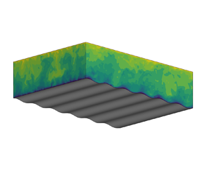
where  $x_j (j=1,2,3)=(x,y,z)$ denote the Cartesian coordinates in the streamwise, spanwise and vertical directions, respectively, as illustrated in figure 1, $u_j (j=1,2,3)=(u,v,w)$ are the components of the filtered velocity in the LES at the grid scale, $p$ is the filtered modified pressure, $\tau _{jm}^d$ is the trace-free part of the subgrid-scale (SGS) stress tensor, $\rho _a$ is the density of air and $\nu$ is the air kinematic viscosity. At the water surface, a progressive water wave is imposed as the Dirichlet boundary condition for the airflow, $u_i(z=\eta )= (u_s, v_s, w_s)$, where $\eta$ is the surface-wave elevation and $(u_s, v_s, w_s)$ is the orbital velocity of the wave at the water surface, given as
 \begin{gather} \eta(x,y,t) = a\sin k(x-ct), \end{gather}
 \begin{gather}u_s(x,y,t) = akc\sin k(x-ct), \end{gather}
 \begin{gather}v_s(x,y,t) = 0, \end{gather}
 \begin{gather}w_s(x,y,t) ={-} akc\cos k(x-ct), \end{gather}
where  $a$ is the amplitude of the surface wave, $k=2{\rm \pi} /\lambda$ is its wavenumber, $\lambda$ is its wavelength and $c$ is its phase speed. In (2.3)–(2.6), an Airy wave solution for deep water waves is adopted. In the case of nonlinear waves, such as a Stokes wave, the effect of nonlinearity by the higher harmonics is of $O((ak)^2)$. In the linear analysis of the wave-induced airflow performed in later sections, the $O((ak)^2)$ terms in the governing equations are omitted. As explained in Cao et al. (Reference Cao, Deng and Shen2020), to be consistent, we only consider the dominant Fourier component in the water-wave solution.

Figure 1. Sketch of LES configuration of turbulent wind following fast-propagating water waves. A three-dimensional wind field is driven by a constant velocity  $U_0$ applied at the top boundary and flows over a plane propagating surface-wave train. The surface wave propagates in the $x$-direction, with a wavelength $\lambda$ and a phase speed $c$. The Dirichlet boundary condition is employed at the wave surface and periodic boundary conditions are applied in the horizontal directions.
In the simulation, the governing equations (2.1) and (2.2) in the physical space are transformed to the rectangular computational space such that
 \begin{equation} \tau=t,\quad \xi=x,\quad \psi=y,\quad \zeta=z+g(\zeta)\eta, \quad \mbox{where}\ g(\zeta) = \frac{\zeta}{L_z}-1, \end{equation}
where  $(\xi , \psi , \zeta , \tau )$ are the spatial and time coordinates in the computational space, $L_z$ is the mean physical domain height and $g(\zeta )$ denotes the transformation function. The Jacobian matrix corresponding to the spatial derivative transformation in (2.7a–d) is
 \begin{equation} \boldsymbol{J}=\left[ \begin{array}{ccc} \displaystyle \dfrac{\partial{\xi}}{\partial x} & \displaystyle \dfrac{\partial{\xi}}{\partial y} & \displaystyle \dfrac{\partial{\xi}}{\partial z} \\ \displaystyle \dfrac{\partial{\psi}}{\partial x} & \displaystyle \dfrac{\partial{\psi}}{\partial y} & \displaystyle \dfrac{\partial{\psi}}{\partial z} \\ \displaystyle \dfrac{\partial{\zeta}}{\partial x} & \displaystyle \dfrac{\partial{\zeta}}{\partial y} & \displaystyle \dfrac{\partial{\zeta}}{\partial z} \end{array} \right] =\left[ \begin{array}{cccc} 1 & 0 & 0 \\ 0 & 1 & 0 \\ \displaystyle \dfrac{g\eta_\xi} {1-g_\zeta \eta} & \displaystyle \dfrac{g\eta_\psi} {1-g_\zeta \eta} & \displaystyle \dfrac{1} {1-g_\zeta \eta} \end{array} \right], \end{equation}
where  $g_\zeta = \mathrm {d} g / \mathrm {d} \zeta$. The transformation of time derivative between the computational space and the physical space in (2.7a–d) caused by the surface-wave motion is defined as
 \begin{equation} \frac{\partial}{\partial t} = \frac{\partial}{\partial \tau} + \frac{\partial{\xi_j}}{\partial t} \frac{\partial}{\partial \xi_j} = \frac{\partial}{\partial \tau} + \frac{\partial{\zeta}}{\partial t} \frac{\partial}{\partial \zeta}, \quad \mbox{where}\ \frac{\partial{\zeta}}{\partial t} = \frac{g\eta_\tau} {1-g_\zeta \eta}. \end{equation}
Then the LES equations (2.1) and (2.2) in the computational space become
 \begin{gather} J_{pj} \frac{\partial u_j}{\partial \xi_p} = 0, \end{gather}
 \begin{gather}\frac{\partial u_j}{\partial \tau} + \delta_{p3} \frac{\partial{\zeta}}{\partial t} \frac{\partial u_j}{\partial \xi_p} + J_{lp} \frac{\partial (u_j u_p)}{\partial \xi_l} ={-} \frac{J_{lj} }{\rho_a} \frac{\partial p}{\partial \xi_l} + J_{lp} \frac{\partial \tau_{jp}^d}{\partial \xi_l} + \nu J_{np} \frac{\partial}{\partial{\xi_n}} \left( J_{lp} \frac{\partial u_j}{\partial{\xi_l}} \right), \end{gather}
where  $J_{lp}$ is the $(l,p)$ entry of the mapping matrix $\boldsymbol {J}$ and $\delta _{lm}$ is the Kronecker delta. The transformed LES equations (2.10) and (2.11) are discretised and solved in computational space. Specifically, in the $(\xi -\psi )$ plane, a Fourier-series-based pseudo-spectral method is used for discretisation with evenly spaced grid points. In the $\zeta$-direction, a second-order finite-difference method is employed with grid points clustered towards the upper and lower boundaries. To calculate the SGS stress tensor, the dynamic Smagorinsky model is used (Smagorinsky Reference Smagorinsky1963; Germano et al. Reference Germano, Piomelli, Moin and Cabot1991; Lilly Reference Lilly1992). The detailed numerical procedure and extensive validations can be found in our previous studies of turbulent wind–wave interactions (Yang & Shen Reference Yang and Shen2010, Reference Yang and Shen2011; Yang, Meneveau & Shen Reference Yang, Meneveau and Shen2013; Hao & Shen Reference Hao and Shen2019; Cao et al. Reference Cao, Deng and Shen2020).
As sketched in figure 1, the turbulent wind is driven by an external velocity at the top of the simulation domain,  $(u, v, w) = (U_0, 0, 0)$; a canonical set-up in the simulations of turbulent airflows over surface waves (e.g. Sullivan et al. Reference Sullivan, McWilliams and Moeng2000; Druzhinin et al. Reference Druzhinin, Troitskaya and Zilitinkevich2012; Cao et al. Reference Cao, Deng and Shen2020). In the present study, the wave age $c/U_0$ varies between $0.1$ and $1.4$, and two wave-steepness values are considered, $ak=0.10$ and $0.15$ (table 1). The wave steepness in the present study is within the range of values adopted in the previous studies of wind over fast waves, e.g. $ak = 0.10$ in Sullivan et al. (Reference Sullivan, McWilliams and Moeng2000), $ak=0.2$ in Hanley & Belcher (Reference Hanley and Belcher2008), $ak=0.10$ and $0.25$ in Yang & Shen (Reference Yang and Shen2010), $ak=0.05\text {--}0.4$ in Jiang et al. (Reference Jiang, Sullivan, Wang, Doyle and Vincent2016) and $ak = 0.10$ in Åkervik & Vartdal (Reference Åkervik and Vartdal2019). The Reynolds number based on the wavelength of the surface wave and the top-driven velocity, $U_0\lambda /\nu$, is 30 000, which is higher than the values 8800–15 000 in the previous DNS of wind over water waves (e.g. Sullivan et al. Reference Sullivan, McWilliams and Moeng2000; Yang & Shen Reference Yang and Shen2010; Druzhinin et al. Reference Druzhinin, Troitskaya and Zilitinkevich2012). The Reynolds number based on the air friction velocity $u_\tau$, i.e. $u_\tau \lambda /\nu$, is obtained a posterior and is summarised in table 1, and is comparable with values in the wall-resolved LES study by Åkervik & Vartdal (Reference Åkervik and Vartdal2019). In the present study, $u_\tau$ is defined using the mean viscous shear stress at the top boundary $\tau _s$, which equals the mean total stress in the streamwise direction at any given height in the wave boundary layer, as $u_\tau =\sqrt {\tau _s/\rho _a}$. Following the previous studies (e.g. Sullivan et al. Reference Sullivan, McWilliams and Moeng2000; Druzhinin et al. Reference Druzhinin, Troitskaya and Zilitinkevich2012; Cao et al. Reference Cao, Deng and Shen2020), a simulation domain of the size $(L_x, L_y, L_z) = (6\lambda , 4\lambda , \lambda )$ is adopted for the wind turbulence. The wind field is discretised in the computational space with $384^2\times 193$ grid points, providing a resolution of $\Delta \xi /(\nu / u_\tau ) < 21$, $\Delta \psi /(\nu / u_\tau ) < 14$ and $\Delta \zeta _{{min}}/(\nu / u_\tau ) < 0.2$, where $\Delta \zeta _{{min}}$ is the minimum grid space in the $\zeta$-direction near the boundaries. The grid resolution in all cases satisfies the requirement of the wall-resolved LES specified by Choi & Moin (Reference Choi and Moin2012). The parameters and resolution of the LES cases in this study are summarised and listed in table 1.
Table 1. List of LES cases for turbulent wind over progressive water waves. The wind field is discretised with  $(N_x, N_y, N_z)=(384, 384, 193)$ grid points in the ( $\xi , \psi , \zeta$) directions, respectively. The bulk Reynolds number $U_0\lambda /\nu$ is prescribed as 30 000 for all of the wave cases, while $u_\tau$, $u_\tau \lambda /\nu$ and the grid resolution in wall units are obtained a posterior. Here, the superscript ‘ $+$’ denotes normalisation by the viscous length scale $\nu /u_\tau$.

3. Mean velocity and turbulence statistics of airflow
In this section, we first examine the mean velocity and turbulence statistics in the airflow for different wave ages using the LES data. To explain the variation of airflow velocity with wave age, we analyse the mean momentum equation for the wind, with a focus on the direction of momentum transfer between the wind and the wave at the water surface.
To analyse the airflow statistics, we adopt the triple decomposition (Hussain & Reynolds Reference Hussain and Reynolds1970) for an instantaneous physical quantity in the airflow,
 \begin{equation} f=\bar{f}(\xi, \zeta) + f'(\xi, \psi, \zeta, t) = \langle\, f \rangle(\zeta) + \tilde{f}(\xi, \zeta) + f'(\xi, \psi, \zeta, t), \end{equation}
where  $f$ denotes an arbitrary physical quantity, $\bar {f}$ is its phase-averaged part, $\langle\, f \rangle$ is its mean value, which is obtained through the average in time and over the $(\xi , \psi )$ plane, $\tilde {f}=\bar {f}-\langle\, f \rangle$ is its wave-induced fluctuation and $f'=f-\bar {f}$ is its turbulent fluctuation. We note that $\tilde {f}$ in (3.1) is defined based on the computational curvilinear coordinates as in previous studies (e.g. Hsu et al. Reference Hsu, Hsu and Street1981; Belcher & Hunt Reference Belcher and Hunt1993; Sullivan et al. Reference Sullivan, McWilliams and Moeng2000; Druzhinin et al. Reference Druzhinin, Troitskaya and Zilitinkevich2012; Buckley & Veron Reference Buckley and Veron2016; Åkervik & Vartdal Reference Åkervik and Vartdal2019; Cao et al. Reference Cao, Deng and Shen2020). For periodic waves, $\tilde {f}$ can be represented using its Fourier coefficient $\hat {f}$, as
 \begin{equation} \tilde{f}=\hat{f}\mathrm{e}^{\mathrm{i}k\xi} + \hat{f}^*\mathrm{e}^{-\mathrm{i}k\xi}=2\,\textrm{Re} \left[\,\hat{f} \right]\cos(k\xi)-2\textrm{Im}\left[\,\hat{f} \right]\sin(k\xi) = 2|\, \hat{f}|\sin(k\xi-\phi_{\tilde{f}\tilde{\eta}}). \end{equation}
Here ‘ $|\cdot |$’ is the modulus operator for complex numbers and $\phi _{\tilde {f}\tilde {\eta }}=\arctan (\textrm {Re}[\,\hat{f}]/\textrm {Im}[\,\hat{f}])$ is the phase difference from the surface-wave profile $\tilde {\eta } =a\sin (k\xi )$ and $\hat {f}^*$ is the complex conjugate of $\hat {f}$.
Figure 2 shows the mean wind velocity  $\langle u \rangle$ and turbulent air velocity variance for different wave age $c/U_0$. Here, we note that in this study, when illustrating the characteristics of airflow statistics, we only present the results of $ak=0.15$ as representative cases for paper length considerations. But both the $ak=0.1$ and the $ak=0.15$ results will be utilised when the mechanisms underlying the wave-induced airflow are elucidated. Figure 2(a) shows that as the wave propagates faster, the mean wind velocity increases, suggesting the diminishing of the blocking effect on the airflow by the wave. In contrast, figure 2(b–d) show that all of the three components of the turbulent air velocity variance decreases appreciably as $c/U_0$ increases. The weakening of turbulence intensity is also reflected in the decreasing of $u_\tau$, with increasing wave speed (table 1). When normalised by $u_\tau$, the difference in the turbulence variance is small. Interestingly, it is observed that the turbulence-intensity profiles become more symmetric with increasing wave age. For instance, in the cases $(c/U_0, c/u_\tau )=(0.4, 15.38)$ and $(c/U_0, c/u_\tau )=(1.2, 54.30)$, the profiles at the top and bottom are similar. This trend of turbulence-intensity profiles is worthy of further investigation in the future. For a specific wave age for fast waves, the higher the wave steepness, the larger the mean wind velocity and the weaker the turbulence variance (which can be seen by comparing $c/U_{\lambda /2}$ and $u_\tau$ for the same $c/U_0$ between different wave steepness in table 1), indicating that the fast wave effects increase with the wave steepness.

Figure 2. Mean wind velocity and turbulent air velocity variance: (a)  $\langle u \rangle$; (b) $\langle u'^2 \rangle ^{{1}/{2}}$; (c) $\langle v'^2 \rangle ^{{1}/{2}}$; and (d) $\langle w'^2 \rangle ^{{1}/{2}}$. The wave conditions shown are: black solid line, $(c/U_0, c/u_\tau )=(0.1, 3.46)$; cyan solid line, $(c/U_0, c/u_\tau )=(0.4, 15.38)$; blue solid line, $(c/U_0, c/u_\tau )=(1.2, 54.30)$. Results for $ak=0.15$. The results are normalised by $U_0$.
The increase of mean airflow velocity, as the wave age increases, is caused by the changed direction of wind–wave momentum flux. To examine the momentum transfer, we analyse the mean airflow momentum equation (Hara & Sullivan Reference Hara and Sullivan2015; Cao et al. Reference Cao, Deng and Shen2020)
 \begin{equation} \langle \tau_{13}^w \rangle+\langle \tau_{13}^p \rangle + \langle \tau_{13} \rangle+ \langle \tau_{13}^v \rangle = \langle \tau_{tot} \rangle= u_\tau^2. \end{equation}
Here,  $\tau ^w_{jm}=-\tilde {u}_j\tilde {U}_m$ is the wave-induced stress with $U_m=J^{-1} \cdot u_j \cdot {\partial \xi _m}/{\partial x_j}$ being the velocity in the curvilinear coordinates, $J$ being the determinant of the transformation matrix $\boldsymbol {J}$ (2.8) and $\widetilde {(\cdot )}$ defined in (3.1), $\tau _{jm}^p=-J^{-1} \cdot p/\rho _a \cdot \partial \xi _m / \partial x_j$ is the pressure stress, $\tau _{jm}=-u_j'U_m' + J^{-1} \cdot \tau _{jl}^d \cdot \partial \xi _m / \partial x_l$ is the total turbulent stress with $\tau _{jm}^d$ being the SGS stress tensor in (2.2), $\tau _{jm}^v=-J^{-1} \cdot \sigma _{jl} \cdot \partial \xi _m / \partial x_l$ is the viscous stress with $\sigma _{jm}=-2\nu S_{jm}$ and $S_{jm}=(\partial u_j / \partial x_m+\partial u_m / \partial x_j)/2$ and $\tau _{tot}$ is summation of all of the stresses.
Figure 3 presents the mean stress terms in (3.3) for different wave age  $c/U_0$. For all three of the wave conditions, the mean total stress is constant and equals $u_\tau ^2$ at any given height. At the wave surface, the wave-induced stress $\langle \tau _{13}^w \rangle$ and the turbulent stress $\langle \tau _{13} \rangle$ vanish, and the wave-induced pressure $\langle \tau _{13}^p \rangle$ equals the form drag on the wave, which is the dominant mechanism for the momentum exchange between the wind and the wave (see Belcher & Hunt Reference Belcher and Hunt1998). The $\langle \tau _{13}^p \rangle$ at the water surface reverses its sign as $c/U_0$ increases. Specifically, for the slow wave $(c/U_0, c/u_\tau )=(0.1, 3.46)$ (figure 3a), both the viscous stress $\langle \tau _{13}^v \rangle$ and the wave-induced pressure $\langle \tau _{13}^p \rangle$ are positive at the wave surface, indicating that the momentum flux is from the wind field to the waves. As $c/U_0$ increases, $\langle \tau _{13}^p \rangle$ decreases and then becomes negative. For the intermediate wave $(c/U_0, c/u_\tau )=(0.4, 15.38)$ (figure 3b), $\langle \tau _{13}^p \rangle$ is negligible and the momentum exchange between the wind and the wave is also small. Under the fast wave condition $(c/U_0, c/u_\tau )=(1.2, 54.30)$ (figure 3c), $\langle \tau _{13}^p \rangle$ is negative, suggesting that the wave loses momentum to the wind field. Meanwhile, $\langle \tau _{13}^v \rangle$ is greater than $u_\tau ^2$ near the wave surface owing to the negative $\langle \tau _{13}^p \rangle$. Therefore, the change of the sign of form drag on the wave surface results in the larger mean airflow velocity as the wave speed increases. Figure 3 also shows that the mean viscous stress $\langle \tau _{13}^v \rangle$ is mainly generated by the vertical gradient of mean airflow velocity and can be approximated by $\nu \,\mathrm {d}\langle u \rangle /\mathrm {d} \zeta$. In other words, the mean wind velocity profile $\langle u \rangle$ is shaped by the mean stresses in the wave boundary layer.

Figure 3. Stress terms in the mean momentum equation (3.3): green dash dotted line, wave-induced stress  $\langle \tau _{13}^w \rangle$; blue dashed line, wave-induced pressure $\langle \tau _{13}^p \rangle$; red solid line, turbulent stress $\langle \tau _{13} \rangle$; orange dashed line, viscous stress $\langle \tau _{13}^v \rangle$; solid black line, approximation of $\langle \tau _{13}^v \rangle$ by $\nu \,\mathrm {d}\langle u \rangle /\mathrm {d} \zeta$; black thin dashed line, total stress $\langle \tau _{tot} \rangle$. The wave conditions shown are: (a) $(c/U_0, c/u_\tau )=(0.1, 3.46)$; (b) $(c/U_0, c/u_\tau )=(0.4, 15.38)$; and (c) $(c/U_0, c/u_\tau )=(1.2, 54.30)$. Results for $ak=0.15$. The results are normalised by $u_\tau ^2$.
To summarise this section, the LES results have shown that as the wave age increases, the mean wind velocity increases and the airflow turbulence intensity is weakened. The analyses of mean airflow equation illustrate that the form drag on the wave surface transits from positive, for slow waves, to negative for fast waves, which causes the larger mean airflow velocity in the latter case.
4. Features and magnitude of wave effects on airflow
In this section, we investigate the features and perform magnitude-scaling analyses of the wave-induced perturbations to the airflow using the LES data. We first examine in § 4.1 the wave effects on the airflow velocity and pressure. Then in § 4.2, the wave-induced perturbations to the airflow turbulence variance and turbulent shear stress are analysed.
4.1. Wave-induced velocity and pressure
In this subsection, we focus on the wave-induced velocity and pressure in the wind field. Figure 4 presents the wave-induced vertical velocity  $\tilde {w}$ for different wave ages. It is shown that the structure of $\tilde {w}$ varies substantially with $c/U_0$, indicating that the physical process producing $\tilde {w}$ depends significantly on $c/U_0$. For the slow wave with $(c/U_0, c/u_\tau )=(0.1, 3.46)$ (figure 4a), away from the surface, $\tilde {w}$ is mostly positive above the windward face and negative above the leeward face, without displaying antisymmetry across the wave crest. The $\tilde {w}$ for slow waves ( $c \simeq u_\tau$) is produced by the airflow blocked by the windward face of the wave owing to the low wave speed. The airflow goes upward along the wave windward surface and therefore has a positive $\tilde {w}$ there. However, when $c \gg u_\tau$, the wave surface no longer blocks the overlying airflow. As shown, for the intermediate wave with $(c/U_0, c/u_\tau )=(0.4, 15.38)$ (figure 4b), the structure of $\tilde {w}$ is remarkably different from that of the slow wave. Specifically, in the near surface region, $\tilde {w}$ exhibits a nearly antisymmetric spatial structure about the wave crest, namely, positive over the leeward side and negative over the windward side with a comparable magnitude. The antisymmetric distribution of $\tilde {w}$ is also present in the fast wave case with $(c/U_0, c/u_\tau )=(1.2, 54.30)$ (figure 4c), but with a much larger amplitude and extends to a much higher altitude in the airflow.

Figure 4. Wave-induced vertical air velocity  $\tilde {w}/(akU_0)$ for the wave conditions: (a) $(c/U_0, c/u_\tau )=(0.1, 3.46)$; (b) $(c/U_0, c/u_\tau )=(0.4, 15.38)$; (c) $(c/U_0, c/u_\tau )= (1.2, 54.30)$. Results for ${ak=0.15}$.
The nearly antisymmetric  $\tilde {w}$ in the intermediate (figure 4b) and fast (figure 4c) wave cases indicates that it is associated with the airflow perturbation induced by the vertical wave movement, i.e. $w_s$ (2.6). At the surface, the vertical air velocity satisfies the Dirichlet boundary condition (2.6) and therefore $\tilde {w}(\zeta =0)=\tilde {w}_s=-akc \cos (k\xi )$, with $\tilde {\eta }=a\sin (k\xi )$. Therefore, one can expect that at the wave surface, a strong vertical motion of water wave would initiate a strong upward airflow at the leeward face and downward airflow at the windward face, which is confirmed by the LES result of $\tilde {w}$ shown in figures 4(b) and 4(c). Away from the surface, the airflow perturbation induced by the vertical wave motion weakens gradually and thus the magnitude of $\tilde {w}$ decays with height. The previously described mechanism for the occurrence of $\tilde {w}$ indicates that $\tilde {w}$ has an order of magnitude of $akc$ for intermediate and fast waves. In particular, when the wave speed $c \gtrsim U_0$, the magnitude of $\tilde {w}$ near the wave surface has a magnitude comparable to $akU_0$. Therefore, in figure 4(c) with $(c/U_0, c/u_\tau )=(1.2, 54.30)$, $\tilde {w}/(akU_0)$ has a magnitude of approximately $1$, which is significantly larger than that shown in figures 4(a) and 4(b).
Figure 5 shows the wave-induced streamwise air velocity  $\tilde {u}$ for different $c/U_0$. At the low wave age with $(c/U_0, c/u_\tau )=(0.1, 3.46)$ (figure 5a), $\tilde {u}$ has a strong positive value at the windward side near the wave crest, caused by the streamwise velocity acceleration associated with the narrowing of cross-section of the air passage on the windward side of the slow wave. For the intermediate wave with $(c/U_0, c/u_\tau )=(0.4, 15.38)$ (figure 5b), $\tilde {u}$ has a large magnitude only in a very thin region above the surface. For the fast wave with $(c/U_0, c/u_\tau )=(1.2, 54.30)$ (figure 5c), away from the surface, $\tilde {u}$ is nearly in antiphase with the wave elevation, namely, a positive $\tilde {u}$ above the wave trough and a negative $\tilde {u}$ above the wave crest, which appears contrary to the airflow perturbation induced by the streamwise component of the wave kinematics. Specifically, at the wave surface, $\tilde {u}(\zeta =0)=\tilde {u}_s= akc \sin (k\xi )$, with $\tilde {\eta }=a\sin (k\xi )$, according to the Dirichlet boundary condition (2.4). Therefore, the streamwise motion of water wave induces a $\tilde {u}$ in phase with the wave elevation at the water surface (because $akc>0$), which is not exhibited by the structure of $\tilde {u}$ away from the surface in figure 5(c). In fact, for fast waves, the effect of the boundary condition (2.4) on $\tilde {u}$ is limited within a very thin region in the airflow and, thus, is not obvious in figure 5(c) (see more detailed discussions in § 6). Away from the surface, $\tilde {u}$ is mainly produced by the airflow perturbation induced by the vertical wave motion (figure 4c) through mass conservation as
 \begin{equation} \frac{\partial \tilde{u}}{\partial \xi} ={-} \frac{\partial \tilde{w}}{\partial \zeta} - \frac{\mathrm{d} \langle u \rangle}{\mathrm{d} \zeta} g\tilde{\eta}_{\xi}, \end{equation}
which is derived using (5.4) in § 5 and illustrates how  $\tilde {u}$ can be generated by $\tilde {w}$. Under the fast wave condition $c \gtrsim U_0$, at a vertical length scale $l=O(k^{-1})$, $\partial \tilde {w} / \partial \zeta =O(ak^2c)$ and $\mathrm {d} \langle u \rangle / \mathrm {d} \zeta g \tilde {\eta }_{\xi } = O(ak^2u_\tau )$. Equation (4.1) suggests that away from the surface, $\tilde {u}$ is dominated by $\partial \tilde {w} / \partial \zeta$ and therefore $\tilde {u} = O(akc)$. For $c \gtrsim U_0$, the magnitude of $\tilde {u}$ is expected to be comparable to $akU_0$, which is reflected in the result in figure 5(c). In addition, because $\tilde {w}$ has the form of $-\cos (k\xi )$ and decays with $\zeta$ (figure 4c), the dominance of $\partial \tilde {w} / \partial \zeta$ in (4.1) indicates that above the wave, $\tilde {u}$ is in antiphase with wave surface, which is consistent with figure 5(c).

Figure 5. Wave-induced streamwise air velocity  $\tilde {u}/(ak U_0)$ for the wave conditions: (a) $(c/U_0, c/u_\tau ) =(0.1, 3.46)$; (b) $(c/U_0, c/u_\tau )=(0.4, 15.38)$; (c) $(c/U_0, c/u_\tau )=(1.2, 54.30)$. Results for $ak=0.15$.
Figure 6 shows the wave-induced air pressure  $\tilde {p}$ for different $c/U_0$. At low wave age with $(c/U_0, c/u_\tau )=(0.1, 3.46)$ (figure 6a), $\tilde {p}$ is highly asymmetric about the wave crest, positive at the windward face and negative at the leeward face, which generates a strong form drag on the wave surface to transfer the momentum from the wind to wave. For the intermediate wave with $(c/U_0, c/u_\tau )=(0.4, 15.38)$ (figure 6b), similar to $\tilde {w}$ and $\tilde {u}$, $\tilde {p}$ is significant only within a thin region near the surface. For the fast wave with $(c/U_0, c/u_\tau )=(1.2, 54.30)$ (figure 6c), similar to $\tilde {u}$, $\tilde {p}$ is strong and is nearly in antiphase with the wave surface, owing to the vertical wave motion-induced airflow. To illustrate this point, we obtain the dominant mechanism for producing $\tilde {p}$ using the vertical momentum equation of the wave-induced airflow, which is (detailed derivation is given in § 5.1)
 \begin{equation} (\langle u \rangle -c )\frac{\partial \tilde{w}}{\partial \xi} \approx{-} \frac{\partial \tilde{p}}{\partial \zeta}, \end{equation}
and the solution follows,
 \begin{equation} \tilde{p} \vert_\zeta \approx \int_{\zeta}^{\infty} (\langle u \rangle -c )\frac{\partial \tilde{w}}{\partial \xi} \,\mathrm{d} \zeta. \end{equation}
Since for the fast wave,  $\tilde {w}$ is nearly in antiphase with the wave slope $\tilde {\eta }_{\xi }$ as shown in figure 4(c) and $\langle u \rangle -c < 0$, (4.3) illustrates that $\tilde {p}$ is nearly in antiphase with the wave elevation. Meanwhile, for $c \gtrsim U_0$, by considering $\tilde {w} = O(akc)$ and $U_0/2 \lesssim |\langle u \rangle -c|$ when $\zeta /\lambda < 0.5$, we obtain that $\tilde {p}=O(ak \rho _a c U_0)$ based on (4.3). This result explains why $\tilde {p}/ak \rho _a U_0^2$ has a magnitude of approximately 1 for $(c/U_0, c/u_\tau )=(1.2, 54.30)$ in figure 6(c).

Figure 6. Wave-induced air pressure  $\tilde {p}/(ak\rho _a U_0^2)$ for the wave conditions: (a) $(c/U_0, c/u_\tau )=(0.1, 3.46)$; (b) $(c/U_0, c/u_\tau )=(0.4, 15.38)$; (c) $(c/U_0, c/u_\tau )=(1.2, 54.30)$. Results for $ak=0.15$.
To summarise this subsection, the LES results have shown that the wave-induced airflow is governed by different physical processes between slow waves and fast waves. Specifically, for slow waves, the wave-induced airflow occurs as a result of the blocking effect of the wave surface, while for fast waves it results from the airflow perturbation induced by the vertical motion of the wave. Therefore, when the wave speed  $c$ is comparable with, or larger than the outer velocity $U_0$, i.e. $c \gtrsim U_0$, the wave-induced velocity and pressure scale as $\tilde {u}=O(akc)$, $\tilde {w}=O(akc)$ and $\tilde {p}=O(ak \rho _a c U_0)$, respectively, which are significantly stronger than those of slow waves.
4.2. Wave-induced turbulence variance and turbulent shear stress
In this subsection, we examine the spatial structure and magnitude of the wave-induced turbulence variance and turbulent shear stress. Figure 7 presents the distribution of wave-induced turbulence variance  $\widetilde {u'u'}+\widetilde {v'v'}+\widetilde {w'w'}=\overline {u'u'} -\langle u'u'\rangle + \overline {v'v'} - \langle v'v' \rangle + \overline {w'w'} - \langle w'w' \rangle$ for different $c/U_0$. In general, $\widetilde {u'u'}+\widetilde {v'v'}+\widetilde {w'w'}$ reflects the wave effects on the turbulence variance in the air, which can, in turn, affect the behaviour of wave-induced airflow as illustrated in the previous studies on wind over slow waves (e.g. Belcher & Hunt Reference Belcher and Hunt1993; Miles Reference Miles1993, Reference Miles1996). As shown in the figure, the slow wave with $(c/U_0, c/u_\tau )=(0.1, 3.46)$ induces a strong positive $\widetilde {u'u'}+\widetilde {v'v'}+\widetilde {w'w'}$ above the leeward face of the wave (figure 7a). Buckley & Veron (Reference Buckley and Veron2016) attribute this enhanced turbulence intensity to sporadic airflow separation past the wave crest. By contrast, the intermediate wave with $(c/U_0, c/u_\tau )=(0.4, 15.38)$ intensifies the turbulence variance at the windward face of the wave, and suppresses the turbulence variance at the leeward face (figure 7b). As the wave propagates faster with $(c/U_0, c/u_\tau )=(1.2, 54.30)$, the regions corresponding to the intensified and suppressed turbulence variance shift farther upstream, such that $\widetilde {u'u'}+\widetilde {v'v'}+\widetilde {w'w'}$ displays a positive value over the wave trough and a negative value over the wave crest, as shown in figure 7(c). Importantly, it is observed that, unlike $\tilde {w}$, $\tilde {u}$ and $\tilde {p}$, the magnitudes of wave-induced turbulence variance normalised by $u_\tau ^2$ are comparable for different $c/U_0$ with a magnitude of $O(1)$, or $\widetilde {u'u'}+\widetilde {v'v'}+\widetilde {w'w'}=O(u_\tau ^2)$. This observation is utilised in § 5.2 to show that for fast waves, the effects of nonlinear forcing on the wave-induced airflow are negligible.

Figure 7. Wave-induced turbulence variance  $(\widetilde {u'u'}+\widetilde {v'v'}+\widetilde {w'w'})/u_\tau ^2$ for the wave conditions: (a) $(c/U_0, c/u_\tau )=(0.1, 3.46)$; (b) $(c/U_0, c/u_\tau )=(0.4, 15.38)$; and (c) $(c/U_0, c/u_\tau )=(1.2, 54.30)$. Results for $ak=0.15$.
Figure 8 compares the wave-induced turbulent shear stress  $-\widetilde {u'w'} = -\overline {u'w'}-\langle -u'w'\rangle$ for the three wave ages. At the small wave age with $(c/U_0, c/u_\tau )=(0.1, 3.46)$, similar to the turbulence variance (figure 7a), the turbulent shear stress is enhanced above the leeward face of the wave (figure 8a), owing to the effect of intermittent airflow separation downstream of the wave crest (Buckley & Veron Reference Buckley and Veron2016). For the intermediate wave age with $(c/U_0, c/u_\tau )=(0.4, 15.38)$, $-\widetilde {u'w'}$ has a negative value above the windward face and a positive value above the leeward face, with an almost antisymmetric spatial structure across the wave crest (figure 8b). Compared with case $(c/U_0, c/u_\tau )=(0.4, 15.38)$, at the high wave age with $(c/U_0, c/u_\tau )=(1.2, 54.30)$, $-\widetilde {u'w'}$ exhibits a similar spatial distribution, but is limited to a slightly thinner region in the airflow (figure 8c). Similar to $\widetilde {u'u'}+\widetilde {v'v'}+\widetilde {w'w'}$, the LES results suggest that for different wave ages, $-\widetilde {u'w'}=O(u_\tau ^2)$. The previous results demonstrate that, contrary to the wave-induced velocity and pressure, which are significantly stronger in the fast wave case than in the slow wave case, $\widetilde {u'u'}+\widetilde {v'v'}+\widetilde {w'w'}$ and $-\widetilde {u'w'}$ have magnitudes comparable for different wave speeds.

Figure 8. Wave-induced turbulent shear stress  $-\widetilde {u'w'}/u_\tau ^2$ for the wave conditions: (a) $(c/U_0, c/u_\tau )= (0.1, 3.46)$; (b) $(c/U_0, c/u_\tau )=(0.4, 15.38)$; and (c) $(c/U_0, c/u_\tau )=(1.2, 54.30)$. Results for ${ak=0.15}$.
To conclude § 4, the LES results indicate that for wind over fast waves, the wave-coherent airflow is dominated by the vertical wave motion-induced air motion, which is much stronger than for wind over slow waves. By contrast, compared with the slow wave, the modulation of turbulence variance and turbulent stress by the fast waves are not strengthened. These results together suggest that the effects of wave-induced turbulent stress on the wave-induced airflow become relatively weaker as the wave propagates faster. In § 5, we develop a linear-analysis framework for the wave effects on the wind, based on which the fast wave-induced airflow is explained theoretically in § 6.
5. Development of linear-analysis framework for wave effects
In this section, we develop a linear-analysis framework for the wave-induced airflow in the turbulent-wave boundary layer by neglecting nonlinear forcing. In § 5.1, a curvilinear model is presented based on non-orthogonal curvilinear coordinates. In § 5.2, we perform a scaling analysis on the effects of nonlinear forcing. In § 5.3, we show that the curvilinear model can be split into two equations to investigate the effects of wave kinematics and body forcing induced by the wave elevation, respectively.
5.1. Non-orthogonal curvilinear model
To capture the wave-induced quantities in the entire region of airflow including the height above the wave trough and below the wave crest, the Cartesian coordinates  $(x,y,z)$ can be transformed to the non-orthogonal curvilinear coordinates $(\xi ,\psi ,\zeta )$, as
 \begin{equation} \xi = x, \quad \psi = y, \quad \zeta = z+g(\zeta)\eta, \end{equation}
where  $g(\zeta )$ can be any function that increases monotonically from the wave surface to the top of the simulation domain (Hsu et al. Reference Hsu, Hsu and Street1981). In the present LES, the computational coordinates (2.7a–d) follow the form of (5.1a–c) with a linear mapping function $g = \zeta /L_z-1$. With the general transformation (5.1a–c) and the properties of phase average, the momentum and continuity equations for the wave-induced airflow can be expressed as (Cao et al. Reference Cao, Deng and Shen2020)
 \begin{align} & (\langle u \rangle -c )\frac{\partial \tilde{u}}{\partial \xi} + (\tilde{w} + (\langle u \rangle -c ) g\tilde{\eta}_{\xi}) \frac{\mathrm{d} \langle u \rangle}{\mathrm{d} \zeta} + \frac{1}{\rho_a} \frac{\partial \tilde{p}}{\partial \xi}\nonumber\\ &\quad = \nu \left(\frac{\partial^2 \tilde{u}}{\partial \zeta^2} - \frac{\partial^2 \tilde{w}}{\partial \xi \partial \zeta}\right) + \nu \frac{\mathrm{d}}{\mathrm{d} \zeta} \left(\frac{\mathrm{d} \langle u \rangle}{\mathrm{d} \zeta} g_\zeta \right) \tilde{\eta} + O((ak)^2) + n.l.f., \end{align}
 $$\begin{gather} (\langle u \rangle -c )\frac{\partial \tilde{w}}{\partial \xi} + \frac{1}{\rho_a} \frac{\partial \tilde{p}}{\partial \zeta} = \nu \left(\frac{\partial^2 \tilde{w}}{\partial \xi^2} + \frac{\partial^2 \tilde{w}}{\partial \zeta^2}\right) + O((ak)^2) + n.l.f., \end{gather}$$
 $$\begin{gather}\frac{\partial \tilde{u}}{\partial \xi} + \frac{\partial \tilde{w}}{\partial \zeta} + \frac{\mathrm{d} \langle u \rangle}{\mathrm{d} \zeta} g\tilde{\eta}_{\xi}= 0 + O((ak)^2), \end{gather}$$
where  $O((ak)^2)$ denotes the neglected second- and higher-order terms (we neglect the correlations between a wave-induced quantity $\tilde {f}$ and $O(ak)^2$ terms, such as $\tilde {\eta }_\xi ^2\tilde {f}$ compared with $\tilde {f}$ (to capture the dominant flow physics only). Here, $g$ is treated as an $O(1)$ quantity), ‘ $n.l.f.$’ represents the neglected nonlinear forcing, namely, the wave-induced fluctuations of the turbulent stress, i.e. $\tilde {\tau }_{jm}$ and the wave-induced fluctuations of the wave-induced stress, i.e. $\tilde {\tau }^w_{jm}$. The effects of $\tilde {\tau }^w_{jm}$ are always small for moderate wave slopes, and the effects of $\tilde {\tau }_{jm}$ are analysed in § 5.2. Note that although (5.2)–(5.4) are on the curvilinear coordinate system, primitive variables in the physical space are used in the equations for more direct illustration of the flow physics.
Next, by eliminating  $\tilde {u}$ and $\tilde {p}$, we can reduce the equation system (5.2)–(5.4) to a single equation for $\tilde {w}$ as (Cao et al. Reference Cao, Deng and Shen2020)
 \begin{align} & -\frac{\nu}{\mathrm{i}k}\left[\frac{\mathrm{d}^4}{\mathrm{d} \zeta^4}-2k^2\frac{\mathrm{d}^2}{\mathrm{d} \zeta^2}+k^4\right]\hat{w}+\left[(\langle u \rangle -c) \left(\frac{\mathrm{d}^2}{\mathrm{d} \zeta^2}-k^2 \right)-\frac{\mathrm{d}^2 \langle u \rangle}{\mathrm{d} \zeta^2} \right]\hat{w}\nonumber\\ &\quad = \nu\hat{\eta}\frac{\mathrm{d}^2}{\mathrm{d} \zeta^2} \left[g \frac{\mathrm{d}^2 \langle u \rangle}{\mathrm{d} \zeta^2} \right] + O((ak)^2) + n.l.f., \end{align}
where  $\hat {w}$ is the Fourier coefficient of $\tilde {w}$ (3.2). The curvilinear equation (5.5) is different from the original Orr–Sommerfeld equation (e.g. Lin Reference Lin1955) in that the presence of the wave elevation $\hat {\eta }$ leads to a forcing term on its right-hand side. To evaluate the relative importance of the right-hand side in (5.5) requires information on the dependence of the mean wind velocity profile on the Reynolds number. However, how to model the mean wind velocity profile as a function of Reynolds number and mean stresses in the turbulent-wave boundary layer is still an open question in the research community and should be investigated in the future.
Equation (5.5) can be solved using the boundary conditions imposed by the wave kinematics, including the Dirichlet boundary conditions for  $\hat {w}$,
 \begin{equation} \left. \hat{w} \right\vert_{\zeta=0} = \hat{w}_s, \quad \left. \hat{w}\right\vert_{\zeta=\infty} = 0, \end{equation}
and the Neumann boundary conditions for  $\mathrm {d} \hat {w} / \mathrm {d} \zeta$, which can be derived from (5.4) and read
 \begin{equation} \left.\frac{\mathrm{d} \hat{w}}{\mathrm{d} \zeta}\right\vert_{\zeta=0}={-}\mathrm{i}k\hat{u}_s-\mathrm{i}k\hat{\eta}\left.\frac{\mathrm{d} \langle u \rangle}{\mathrm{d} \zeta} \right\vert_{\zeta=0}, \quad \left.\frac{\mathrm{d} \hat{w}}{\mathrm{d} \zeta}\right\vert_{\zeta=\infty} = 0, \end{equation}
where  $\hat {u}_s$ and $\hat {w}_s$ are the Fourier coefficients of the streamwise (2.4) and vertical (2.6) components of wave orbital velocity, respectively. In § 6, (5.5) with $g = \zeta /L_z-1$ is numerically solved using the mean wind velocity $\langle u \rangle$ from the LES, and its results are compared with LES data to illustrate the mechanisms for the fast wave-induced airflow.
To evaluate the effects of coordinate systems, in appendix A we further develop a curvilinear model based on the orthogonal curvilinear coordinates (e.g. Sullivan et al. Reference Sullivan, McWilliams and Moeng2000; Buckley & Veron Reference Buckley and Veron2016; Yousefi & Veron Reference Yousefi and Veron2020; Yousefi, Veron & Buckley Reference Yousefi, Veron and Buckley2020),
 \begin{equation} \xi = x-\mathrm{i}a\mathrm{e}^{{-}kz}\mathrm{e}^{\mathrm{i}kx}, \quad \psi = y, \quad \zeta = z- a\mathrm{e}^{{-}kz}\mathrm{e}^{\mathrm{i}kx}. \end{equation}
In appendix B, we compare the solutions of the curvilinear equations with different curvilinear coordinates, and show that the mechanisms of fast wave effects on the airflow revealed by the curvilinear models hold the same.
5.2. Scaling analysis of fast wave-induced turbulent stress effects
In this subsection we perform scaling analysis of the effects of fast wave-induced turbulent stress  $\tilde {\tau }_{jm}$ on the wave-induced momentum equations (5.2) and (5.3). In § 4, the LES results show that for fast waves, $\tilde {w}=O(akc)$, $\tilde {p}=O(ak \rho _a c U_0)$, $\widetilde {u'u'}+\widetilde {v'v'}+\widetilde {w'w'}=O(u_\tau ^2)$ and $-\widetilde {u'w'} = O(u_\tau ^2)$. Based on these results, it can be further shown that in the curvilinear coordinates, the wave-induced turbulent stress satisfies $\tilde {\tau }_{jm} = O(u_\tau ^2)$, which has been neglected in deriving (5.2) and (5.3). By comparing the magnitude of $\tilde {\tau }_{jm}$ with the stress terms in (5.2) and (5.3), we can evaluate the effects of $\tilde {\tau }_{jm}$ on the fast wave-induced airflow.
To investigate the effects of  $\tilde {\tau }_{jm}$, we focus on a vertical length scale $l$ satisfying $kl<1$, because $\widetilde {u'u'}+\widetilde {v'v'}+\widetilde {w'w'}$ (figure 7) and $-\widetilde {u'w'}$ (figure 8) are significant only within this region. To analyse the streamwise momentum equation (5.2), we can reduce it to the following form by using (5.4) to eliminate $\tilde {u}$ as
 \begin{equation} -(\langle u \rangle -c )\frac{\partial \tilde{w}}{\partial \zeta} + \tilde{w} \frac{\mathrm{d} \langle u \rangle}{\mathrm{d} \zeta} + \frac{1}{\rho_a} \frac{\partial \tilde{p}}{\partial \xi} = \nu \left(\frac{\partial^2 \tilde{u}}{\partial \zeta^2} - \frac{\partial^2 \tilde{w}}{\partial \xi \partial \zeta}\right) + \nu \frac{\mathrm{d}}{\mathrm{d} \zeta} \left(\frac{\mathrm{d} \langle u \rangle}{\mathrm{d} \zeta} g_\zeta \right) \tilde{\eta}. \end{equation}
With the results in § 4, we can obtain the following scaling in (5.9),
 \begin{gather} \frac{1/\rho_a \partial \tilde{p}/\partial \xi}{-(\langle u \rangle-c) \partial\tilde{w}/\partial\zeta } \sim \frac{ak c U_0 \cdot k}{ak c U_0/l} = kl, \end{gather}
 \begin{gather}\frac{\tilde{w} \langle u \rangle_\zeta}{-(\langle u \rangle-c) \partial\tilde{w}/\partial\zeta} \sim \frac{akc \langle u \rangle(l) /l}{akcU_0/l} = \frac{\langle u \rangle(l) }{U_0}, \end{gather}
 \begin{gather}\frac{\partial \tilde{\tau}_{11}/\partial \xi}{-(\langle u \rangle-c) \partial\tilde{w}/\partial\zeta} \sim \frac{u_\tau^2 \cdot k }{akcU_0/l} < \frac{u_\tau^2/l}{akcU_0/l} \sim \frac{\partial \tilde{\tau}_{13}/\partial \zeta}{-(\langle u \rangle-c) \partial\tilde{w}/\partial\zeta} \sim \frac{1}{ak} \frac{u_\tau}{U_0} \frac{u_\tau}{c}, \end{gather}
where  $\langle u \rangle (l)$ is the value of $\langle u \rangle$ at $\zeta =l$. Similarly, for the vertical momentum equation (5.3), we have
 \begin{gather} \frac{(\langle u \rangle -c ) \partial \tilde{w}/\partial \xi}{1/\rho_a \partial \tilde{p}/\partial \zeta} \sim \frac{akcU_0 \cdot k }{akcU_0/l} = kl, \end{gather}
 \begin{gather}\frac{\partial \tilde{\tau}_{31}/\partial \xi}{1/\rho_a \partial \tilde{p}/\partial \zeta} \sim \frac{u_\tau^2 \cdot k}{akcU_0/l} < \frac{u_\tau^2/l}{akcU_0/l} \sim \frac{\partial \tilde{\tau}_{33}/\partial \zeta}{1/\rho_a \partial \tilde{p}/\partial \zeta} \sim \frac{1}{ak} \frac{u_\tau}{U_0} \frac{u_\tau}{c}. \end{gather}
In the wave surface layer,  $ak \simeq 0.1$ and $U_0/u_\tau$ is large. Equations (5.10)–(5.12) illustrate that for high wave age $c/u_\tau$, $\partial \tilde {\tau }_{11}/\partial \xi$ and $\partial \tilde {\tau }_{13}/\partial \zeta$ are significantly smaller than $-(\langle u \rangle -c) \partial \tilde {w}/\partial \zeta$ in the streamwise momentum equation (5.9). Likewise, (5.13) and (5.14) demonstrate that for large $c/u_\tau$, $\partial \tilde {\tau }_{31}/\partial \xi$ and $\tilde {\tau }_{33}/\partial \zeta$ have negligible effects compared with $1/\rho _a \cdot \partial \tilde {p}/\partial \zeta$ in the vertical momentum equation (5.3). If $ak \ll 0.1$, the magnitude of $\tilde {\tau }_{jm}$ should be much smaller than $O(u_\tau ^2)$, and we still expect that its effects are much smaller than the wave-induced advection or pressure. These results suggest that for fast waves, the effects of wave-induced turbulent stress $\tilde {\tau }_{jm}$ on the wave-induced airflow are always much smaller than the dominant forcing in the wave-induced momentum equations, which constitutes the physical grounds for neglecting $\tilde {\tau }_{jm}$, i.e.the nonlinear forcing, in the curvilinear equations. The present scaling analyses support the results of Åkervik & Vartdal (Reference Åkervik and Vartdal2019), who found that for high wave age, the forcing induced by the wave-induced velocity and pressure is mainly balanced by the viscous stress, instead of the turbulent stress, indicating a quasi-laminar flow regime. To further verify this finding, they reproduced the LES results using a linear split system.
Finally, we comment on the effect of Reynolds number on the scaling analyses in this section. The foregoing analyses have shown that the ratio of the magnitude of turbulent stress to the magnitude of inertial forcing induced by the wave-induced velocity or the wave-induced pressure scales with  $(u_\tau /U_0)\cdot (u_\tau /c)$ instead of viscosity, as shown by (5.12) and (5.14). Therefore, for high $c/u_\tau$, the trend that the turbulent stress effects become negligible and the inertial forcing will be balanced by either the viscous stress or the wave elevation-induced forcing should hold irrespective of Reynolds number. However, as the Reynolds number increases, $u_\tau /U_0$ decreases and thus the transition to the quasilinear regime might happen at a lower $c/u_\tau$, which is consistent with the conclusions of Åkervik & Vartdal (Reference Åkervik and Vartdal2019).
5.3. Split equations of curvilinear model
In this subsection, we develop split equations for the curvilinear model of the wave effects on airflow. The expressions of the curvilinear model (5.5) and its boundary conditions (5.6a,b) and (5.7a,b), reveal two mechanisms of the impacts of fast waves on the overlying turbulent wind field, namely, the forcing induced by the wave elevation, which is the source term on the right-hand side of (5.5), and the wave orbital velocity, which is shown by the boundary conditions (5.6a,b)–(5.7a,b). To investigate these two mechanisms separately, we can split a curvilinear equation into two separate equations corresponding to the two components of  $\hat {w}$, $\hat {w}^k$ and $\hat {w}^f$, respectively,
 \begin{equation} \hat{w}= \hat{w}^k + \hat{w}^f. \end{equation}
In this equation,  $\hat {w}^k$ and $\hat {w}^f$ are the vertical velocity perturbations associated with the wave kinematics and by the forcing caused by the wave elevation, respectively.
Extracted from (5.5), the equation for  $\hat {w}^k$ has a zero source term on the right-hand side, but is driven by the wave orbital velocity at the wave surface, which is
 \begin{equation} -\frac{\nu}{\mathrm{i}k}\left[\frac{\mathrm{d}^4}{\mathrm{d} \zeta^4}-2k^2\frac{\mathrm{d}^2}{\mathrm{d} \zeta^2}+k^4\right]\hat{w}^k+\left[ (\langle u \rangle -c) \left(\frac{\mathrm{d}^2}{\mathrm{d} \zeta^2}-k^2 \right)-\frac{\mathrm{d}^2 \langle u \rangle}{\mathrm{d} \zeta^2} \right]\hat{w}^k=0, \end{equation}
with the boundary conditions
 \begin{gather} \left. \hat{w}^k \right\vert_{\zeta=0} = \hat{w}_s, \quad \left. \hat{w}^k\right\vert_{\zeta=\infty} = 0, \end{gather}
 \begin{gather}\left.\frac{\mathrm{d} \hat{w}^k}{\mathrm{d} \zeta}\right\vert_{\zeta=0}={-}\mathrm{i} k\hat{u}_s-\mathrm{i}k\hat{\eta}\left.\left(g\frac{\mathrm{d} \langle u \rangle}{\mathrm{d} \zeta}\right) \right\vert_{\zeta=0}, \quad \left.\frac{\mathrm{d} \hat{w}^k}{\mathrm{d} \zeta}\right\vert_{\zeta=\infty} = 0. \end{gather}
The boundary conditions (5.17a,b) and (5.18a,b) are enforced at  $\zeta =0$, because the effects of wave orbital velocity on the airflow are applied on the curved water-wave surface. Therefore, (5.18a,b) implicitly includes some geometrical effects. The extraction of the wave-kinematics effects by (5.16)–(5.18a,b) follows the idea of Åkervik & Vartdal (Reference Åkervik and Vartdal2019), where the particular solution to the kinematics is split from the rest of the response, but with a difference between these two studies. In Åkervik & Vartdal (Reference Åkervik and Vartdal2019), the particular solution to the kinematics does not involve the background shear effect, whereas (5.16)–(5.18a,b) include the background shear effect. If we set the mean wind velocity to be zero, (5.16) reduces to the formulation obtained by Åkervik & Vartdal (Reference Åkervik and Vartdal2019).
The equation for  $\hat {w}^f$ has a non-zero source term on the right-hand side, but is not affected by the wave kinematics at the surface, we write
 \begin{align} & -\frac{\nu}{\mathrm{i}k}\left[\frac{\mathrm{d}^4}{\mathrm{d} \zeta^4}-2k^2\frac{\mathrm{d}^2}{\mathrm{d} \zeta^2}+k^4\right]\hat{w}^f+\left[ (\langle u \rangle -c) \left(\frac{\mathrm{d}^2}{\mathrm{d} \zeta^2}-k^2 \right)-\frac{\mathrm{d}^2 \langle u \rangle}{\mathrm{d} \zeta^2} \right]\hat{w}^f\nonumber\\ &\quad = \nu\hat{\eta}\frac{\mathrm{d}^2}{\mathrm{d} \zeta^2} \left[g \frac{\mathrm{d}^2 \langle u \rangle}{\mathrm{d} \zeta^2} \right], \end{align}
with the homogeneous boundary conditions
 \begin{gather} \left. \hat{w}^f \right\vert_{\zeta=0} = 0, \quad \left. \hat{w}^f\right\vert_{\zeta=\infty} = 0, \end{gather}
 \begin{gather}\left.\frac{\mathrm{d} \hat{w}^f}{\mathrm{d} \zeta}\right\vert_{\zeta=0}= 0, \quad \left.\frac{\mathrm{d} \hat{w}^f}{\mathrm{d} \zeta}\right\vert_{\zeta=\infty} = 0. \end{gather}
Here, it is noted that following the previous studies (e.g. Miles Reference Miles1957; Belcher & Hunt Reference Belcher and Hunt1993; Miles Reference Miles1996; Hara & Sullivan Reference Hara and Sullivan2015), to discuss the mechanisms for wave-induced velocity, it is assumed that the mean wind velocity profile can be modelled through the mean flow momentum equation or it can be obtained experimentally. Therefore, we treat the right-hand side of (5.19) as a forcing to drive the wave-induced velocity, rather than a geometric correction to the mean wind velocity derivative given a specific wave-induced velocity forcing. In §§ 6.1 and 6.2, the equations (5.16)–(5.18a,b) and (5.19)–(5.21a,b) are solved separately, and their solutions are compared with the LES data to elucidate the effects of wave kinematics and forcing by the wave elevation on fast wave-induced airflow.
To conclude § 5, we have developed a linear-analysis framework for the fast wave effects on the overlying turbulent wind field. The scaling analysis shows that for high  $c/u_\tau$, the nonlinear forcing has secondary effects on the wave-induced airflow compared with the advection induced by $\tilde {w}$ and the gradient of $\tilde {p}$. The curvilinear model of the wave boundary layer reveals two mechanisms for the wave effects on the airflow, namely, the wave kinematics and the forcing induced by the wave elevation, which can be investigated separately by the split curvilinear equations.
6. Explanation of fast wave-induced airflow using linear theory
In this section, we analyse the characteristics and the underlying mechanisms of fast wave-induced airflow through the comparisons between the solutions of the curvilinear equations in § 5 and the LES results. The dominant and weak components of the wave-induce airflow are investigated in §§ 6.1 and 6.2, respectively. In § 6.3, we examine the generation of wave-coherent stress in the wind and the form drag on the wave surface. Finally, the effect of wave age on the behaviours of wave-induced airflow is discussed in § 6.4.
To explain the fast wave-induced airflow, we express the wave-induced vertical velocity  $\tilde {w}$, wave-induced streamwise velocity $\tilde {u}$ and wave-induced pressure $\tilde {p}$ using their Fourier coefficients (3.2) as
 \begin{gather} \tilde{w}= 2|\hat{w}| \sin(k\xi-\phi_{\tilde{w}\tilde{\eta}}), \end{gather}
 \begin{gather}\tilde{u}= 2|\hat{u}| \sin(k\xi-\phi_{\tilde{u}\tilde{\eta}}), \end{gather}
 \begin{gather}\tilde{p}= 2|\hat{p}| \sin(k\xi-\phi_{\tilde{p}\tilde{\eta}}), \end{gather}
where  $2|\hat {w}|$, $2|\hat {u}|$ and $2|\hat {p}|$ are the amplitude of $\tilde {w}$, $\tilde {u}$ and $\tilde {p}$, respectively, and $\phi _{\tilde {w}\tilde {\eta }}$, $\phi _{\tilde {u}\tilde {\eta }}$ and $\phi _{\tilde {p}\tilde {\eta }}$ are the phase difference of $\tilde {w}$, $\tilde {u}$ and $\tilde {p}$ with respect to the wave surface $\tilde {\eta }=\sin (k\xi )$, respectively.
Figure 9 compares the phase difference  $\phi _{\tilde {u}\tilde {\eta }}$ (6.2) between the LES results and the solutions of the curvilinear equation (5.5) for the fast waves. In all of the four wave cases shown, the linear solutions agree well with the LES results. It is observed that $\phi _{\tilde {u}\tilde {\eta }} \approx -{\rm \pi}$ only away from the surface, $\zeta / \lambda \geqslant 0.01$, which is consistent with the results in figure 5(c) and suggests that $|\textrm {Im}[\hat {u}]| \gg |\textrm {Re}[\hat {u}]|$ there. At the surface, owing to the no-slip boundary condition $\tilde {u}=ak \sin (k\xi )$ (2.4), it is shown that $\phi _{\tilde {u}\tilde {\eta }}=0$. The results indicate that the direct effect of the boundary condition (2.4) on $\tilde {u}$ is only limited to a very thin region in the airflow, $\zeta / \lambda \leqslant 0.01$. The further analysis of $\phi _{\tilde {w}\tilde {\eta }}$ (6.1) and $\phi _{\tilde {p}\tilde {\eta }}$ (6.3) shows that $\phi _{\tilde {w}\tilde {\eta }} \approx {\rm \pi}/2$ and $\phi _{\tilde {p}\tilde {\eta }} \approx -{\rm \pi}$ throughout the wave boundary layer (results not plotted here for space considerations), consistent with the observation in figures 4(c) and 6(c), respectively. From the definitions of $\phi _{\tilde {w}\tilde {\eta }}$ and $\phi _{\tilde {p}\tilde {\eta }}$ (3.2), it can be deduced that $|\textrm {Re}[\hat {w}]| \gg |\textrm {Im}[\hat {w}]|$ and $|\textrm {Im}[\hat {p}]| \gg |\textrm {Re}[\hat {p}]|$ throughout the wave boundary layer. In the following subsections, the mechanisms for the strong ( $\textrm {Re}[\hat {w}]$, $\textrm {Im}[\hat {u}]$ and $\textrm {Im}[\hat {p}]$), and weak ( $\textrm {Im}[\hat {w}]$, $\textrm {Re}[\hat {u}]$ and $\textrm {Re}[\hat {p}]$) components of fast wave-induced airflow are investigated.

Figure 9. Comparison of the phase difference  $\phi _{\tilde {u}\tilde {\eta }}$ (6.2) between the LES results and the solutions of the curvilinear equation (5.5) for the fast waves. Lines are the LES results: black solid line, $(c/U_0, c/u_\tau )=(0.8, 33.61)$; cyan solid line, $(c/U_0, c/u_\tau )=(1.0, 44.64)$; blue solid line, $(c/U_0, c/u_\tau )=(1.2, 54.30)$; green solid line, $(c/U_0, c/u_\tau )=(1.4, 66.67)$. Symbols are the linear solutions: open black box, $(c/U_0, c/u_\tau )=(0.8, 33.61)$; open cyan box, $(c/U_0, c/u_\tau )=(1.0, 44.64)$; open blue box, $(c/U_0, c/u_\tau )=(1.2, 54.30)$; open green box, $(c/U_0, c/u_\tau )=(1.4, 66.67)$. In all four cases, $ak=0.15$.
6.1. Mechanisms for dominant components of wave-induced airflow
So far, we have demonstrated that for fast waves,  $\textrm {Re}[\hat {w}]$, $\textrm {Im}[\hat {u}]$ and $\textrm {Im}[\hat {p}]$ are the dominant components of $|\hat {w}|$, $|\hat {u}|$ and $|\hat {p}|$, respectively. In this subsection, we explain how they are produced. First, we identify the flow dynamics governing the dominant wave-induced airflow. Figure 10 compares the magnitudes and the dominant components of the wave-induced velocity and pressure between the LES results and the solutions of the curvilinear equation (5.5) for four fast waves. The agreement between the LES results and the linear solutions demonstrates that the dominant components of wave-induced airflow are controlled by linear dynamics. As shown, $|\hat {w}|$ and $|\hat {p}|$ have almost the same magnitudes as $\textrm {Re}[\hat {w}]$ and $\textrm {Im}[\hat {p}]$, respectively, throughout the boundary layer, indicating that the overall structures of $\tilde {w}$ and $\tilde {p}$ are determined by $\textrm {Re}[\hat {w}]$ and $\textrm {Im}[\hat {p}]$, respectively. Because $\textrm {Re}[\hat {w}]$ maintains a negative value and $\textrm {Im}[\hat {p}]$ has a positive sign, using (3.2) we can obtain that $\phi _{\tilde {w}\tilde {\eta }} \approx {\rm \pi}/2$ and $\phi _{\tilde {p}\tilde {\eta }} \approx -{\rm \pi}$, which explains the results shown in figures 4(c) and 6(c), respectively. By contrast, $|\hat {u}|$ has a similar magnitude to $\textrm {Im}[\hat {u}]$ only at $\zeta /\lambda \geqslant 0.01$, indicating that $\textrm {Im}[\hat {u}]$ determines the structure of $\tilde {u}$ there. The positive value of $\textrm {Im}[\hat {u}]$ for $\zeta /\lambda \geqslant 0.01$ suggests that $\phi _{\tilde {u}\tilde {\eta }} \approx -{\rm \pi}$. For $\zeta /\lambda < 0.01$, $\phi _{\tilde {u}\tilde {\eta }}$ transits from zero at the surface to $-{\rm \pi}$ farther away, which is caused by the change of the sign of $\textrm {Im}[\hat {u}]$ across this thin region. These results explain figure 9.

Figure 10. Comparison of the magnitudes (a,c,e) and the dominant components (b,d,f) of wave-induced airflow between the LES results and the solutions of the curvilinear equation (5.5) for the fast waves: (a)  $|\hat {w}|$; (b) $\textrm {Re}[\hat {w}]$; (c) $|\hat {u}|$; (d) $\textrm {Im}[\hat {u}]$; (e) $|\hat {p}|$; and (f) $\textrm {Im}[\hat {p}]$. Lines are the LES results: solid black line, $(c/U_0, c/u_\tau )=(0.8, 33.61)$; solid cyan line, $(c/U_0, c/u_\tau )=(1.0, 44.64)$; solid blue line, $(c/U_0, c/u_\tau )=(1.2, 54.30)$; solid green line, $(c/U_0, c/u_\tau )=(1.4, 66.67)$. Symbols are the linear solutions: open black box, $(c/U_0, c/u_\tau )=(0.8, 33.61)$; open cyan box, $(c/U_0, c/u_\tau )=(1.0, 44.64)$; open blue box, $(c/U_0, c/u_\tau )=(1.2, 54.30)$; open green box, $(c/U_0, c/u_\tau )=(1.4, 66.67)$. Results for $ak=0.15$.
The quasilinear behaviour of the dominant wave-induced airflow suggests that the underlying mechanisms can be explained using the curvilinear models. The key is to identify the physical processes that generate  $\textrm {Re}[\hat {w}]$, which can be elucidated using the split curvilinear equations obtained in § 5.3. As mentioned previously, (5.16) for $\hat {w}^k$ and (5.19) for $\hat {w}^f$ represent the effects of the wave kinematics and the forcing by wave elevation, respectively. Figure 11 compares $\textrm {Re}[\hat {w}^k]$ solved from (5.16), $\textrm {Re}[\hat {w}^f]$ solved from (5.19), and $\textrm {Re}[\hat {w}^k]+\textrm {Re}[\hat {w}^f]$ with the $\textrm {Re}[\hat {w}]$ result from LES for $ak=0.1$ and $0.15$. As shown, for both wave steepnesses, $\textrm {Re}[\hat {w}]$ is contributed to almost entirely by $\textrm {Re}[\hat {w}^k]$ with near zero contribution from $\textrm {Re}[\hat {w}^f]$, indicating that the wave kinematics plays a primary role in perturbing the vertical airflow velocity. To further investigate how the wave kinematics produces $\textrm {Re}[\hat {w}^k]$, we examine the boundary conditions for $\textrm {Re}[\hat {w}^k]$, which can be derived from (5.17a,b) and (5.18a,b), and read
 \begin{equation} \left.\textrm{Re}[\hat{w}^k]\right\vert_{\zeta=0}={-}\frac{1}{2}akc, \quad \left.\frac{\mathrm{d} \,\textrm{Re}[\hat{w}^k] }{\mathrm{d} \zeta}\right\vert_{\zeta=0} ={-}\frac{1}{2}ak^2c - \frac{1}{2}ak\left.\left(g\frac{\mathrm{d} \langle u \rangle}{\mathrm{d} \zeta}\right) \right\vert_{\zeta=0}.\end{equation}
We find that the vertical component of wave orbital velocity  $w_s$ (2.6) initiates a perturbation to the vertical air velocity $\textrm {Re}[\hat {w}^k]$ at the wave surface through the Dirichlet boundary condition (6.4a), and the streamwise component of wave orbital velocity $u_s$ (2.4) only affects the vertical derivative of $\textrm {Re}[\hat {w}^k]$, i.e. $\mathrm {d}\, \textrm {Re}[\hat {w}^k]/\mathrm {d} \zeta$, at the wave surface (6.4b). Away from the wave surface, $\textrm {Re}[\hat {w}^k]$ decays monotonically to zero without changing its sign as shown in figure 11.

Figure 11. Comparison of  $\textrm {Re}[\hat {w}^k]$ solved from (5.16), $\textrm {Re}[\hat {w}^f]$ solved from (5.19), $\textrm {Re}[\hat {w}^k]+\textrm {Re}[\hat {w}^f]$ and the $\textrm {Re}[\hat {w}]$ result from the LES for (a) case $(c/U_0, c/u_\tau , ak)=(1.2, 50.42, 0.10)$ and (b) case $(c/U_0, c/u_\tau , ak)=(1.2, 54.30, 0.15)$. Symbols are blue circle, $\textrm {Re}[\hat {w}^k]$; cyan diamond, $\textrm {Re}[\hat {w}^f]$; open green box, $\textrm {Re}[\hat {w}^k]+\textrm {Re}[\hat {w}^f]$; and solid black line, LES result of $\textrm {Re}[\hat {w}]$. Note that $\textrm {Re}[\hat {w}^k]$ and $\textrm {Re}[\hat {w}^k]+\textrm {Re}[\hat {w}^f]$ collapse together.
Based on the results of  $\textrm {Re}[\hat {w}]$, the mechanisms for the dominant components of wave-induced streamwise air velocity $\textrm {Im}[\hat {u}]$ and air pressure $\textrm {Im}[\hat {p}]$ can also be explained. Specifically, $\textrm {Im}[\hat {u}]$ occurs as a result of mass conservation in response to the $\textrm {Re}[\hat {w}]$-associated airflow perturbation, which can be obtained from the continuity equation (5.4) as
 \begin{equation} \textrm{Im}[\hat{u}] = \frac{1}{k} \frac{\mathrm{d}\,\textrm{Re}[\hat{w}]}{\mathrm{d}\zeta}+\frac{1}{2}ag\frac{\mathrm{d} \langle u \rangle}{\mathrm{d}\zeta}. \end{equation}
Equation (6.5) explains that the changing sign of  $\textrm {Im}[\hat {u}]$ (figure 10d) and the associated variation of $\phi _{\tilde {u}\tilde {\eta }}$ (figure 9) in the wave boundary layer are because the effects of $u_s$ on $\textrm {Im}[\hat {u}]$, through the Dirichlet boundary condition (2.4), are limited to the proximity of the wave surface and the behaviour of $\textrm {Im}[\hat {u}]$ at higher altitude is determined primarily by the $\textrm {Re}[\hat {w}]$-associated airflow. Meanwhile, $\textrm {Im}[\hat {p}]$ is generated through the momentum conservation of the $\textrm {Re}[\hat {w}]$-associated airflow, which can be seen from the contribution to $\textrm {Im}[\hat {p}]$ derived from (5.3)
 \begin{equation} \textrm{Im}[\hat{p}] = \int_\zeta^\infty \left[(\langle u \rangle-c)k\,\textrm{Re}[\hat{w}] - \nu \left(k^2 \,\textrm{Im}[\hat{w}]-\frac{\mathrm{d}^2 \,\textrm{Im}[\hat{w}]}{\mathrm{d}\zeta^2}\right)\right]\mathrm{d}\zeta, \end{equation}
where the second term on the right-hand side denotes the viscous stress effect and is much smaller than the first term. Equation (6.6) shows that a strong  $\textrm {Re}[\hat {w}]$ leads to a large-magnitude $\textrm {Im}[\hat {p}]$ (figure 10f).
As a summary of this subsection, we have discovered that the dominant components of fast wave-induced velocity and pressure are directly driven by the wave kinematics at the water surface and can be described by the curvilinear models. Based on the split curvilinear equations, we have illustrated that the vertical wave motion ( $w_s$) initiates a strong vertical air velocity at the wave surface, which gradually decays away from the wave surface and causes a strong $\textrm {Re}[\hat {w}]$ in the airflow. The $\textrm {Re}[\hat {w}]$ further results in $\textrm {Im}[\hat {u}]$ and $\textrm {Im}[\hat {p}]$ in the air through the conservation of mass and momentum, respectively.
6.2. Mechanisms for weak components of wave-induced airflow
In § 6.1, we have explained the occurrence of  $\textrm {Re}[\hat {w}]$, $\textrm {Im}[\hat {u}]$ and $\textrm {Im}[\hat {p}]$, i.e. the dominant components of the fast wave-induced airflow, using the curvilinear equations of the wave boundary layer. In this subsection, we further investigate the physical processes producing the weak components $\textrm {Im}[\hat {w}]$, $\textrm {Re}[\hat {u}]$ and $\textrm {Re}[\hat {p}]$. To show the flow dynamics governing these weak components of wave-induced airflow, figure 12 compares the profiles of $\textrm {Im}[\hat {w}]$, $\textrm {Re}[\hat {u}]$ and $\textrm {Re}[\hat {p}]$ between the LES results and the solutions of the curvilinear equation (5.5) for the fast waves. In all four of the cases shown, the linear solutions agree well with the LES results, suggesting that similar to their strong counterparts, $\textrm {Im}[\hat {w}]$, $\textrm {Re}[\hat {u}]$ and $\textrm {Re}[\hat {p}]$ are also controlled by linear dynamics. For $\tilde {w}$ and $\tilde {p}$, compared with $\textrm {Re}[\hat {w}]$ and $\textrm {Im}[\hat {p}]$ (figure 10b,f), it is found that $|\textrm {Im}[\hat {w}]|<0.04|\textrm {Re}[\hat {w}]|$ and $|\textrm {Re}[\hat {p}]|<0.04|\textrm {Im}[\hat {p}]|$ throughout the boundary layer (figure 12a,c). Therefore, the contributions from $\textrm {Im}[\hat {w}]$ and $\textrm {Re}[\hat {p}]$ to the magnitude, $|\hat {w}|$ and $|\hat {p}|$ (figure 10a,e) and the phase difference, $\phi _{\tilde {w}\tilde {\eta }}$ and $\phi _{\tilde {p}\tilde {\eta }}$, are negligible. However, for $\tilde {u}$, $\textrm {Re}[\hat {u}]$ (figure 12b) is comparable to $\textrm {Im}[\hat {u}]$ (figure 10d) near the surface, $\zeta /\lambda \leqslant 0.01$ and, therefore, $\phi _{\tilde {u}\tilde {\eta }}$ (figure 9) varies significantly across this thin region. Away from the wave surface, $\zeta /\lambda \geqslant 0.01$, $\textrm {Re}[\hat {u}]$ becomes negligible compared with $\textrm {Im}[\hat {u}]$ and correspondingly, $\phi _{\tilde {u}\tilde {\eta }} \approx -{\rm \pi}$ there (figure 9).

Figure 12. Comparison of the profiles of (a)  $\textrm {Im}[\hat {w}]$, (b) $\textrm {Re}[\hat {u}]$ and (c) $\textrm {Re}[\hat {p}]$ between the LES results and the solutions of the curvilinear equation (5.5) for the fast waves. Lines are the LES results: solid black line, $(c/U_0, c/u_\tau )=(0.8, 33.61)$; solid cyan line, $(c/U_0, c/u_\tau )=(1.0, 44.64)$; solid blue line, $(c/U_0, c/u_\tau )=(1.2, 54.30)$; solid green line, $(c/U_0, c/u_\tau )=(1.4, 66.67)$. Symbols are the linear solutions: open black box, $(c/U_0, c/u_\tau )=(0.8, 33.61)$; open cyan box, $(c/U_0, c/u_\tau )=(1.0, 44.64)$; open blue box, $(c/U_0, c/u_\tau )=(1.2, 54.30)$; open green box, $(c/U_0, c/u_\tau )=(1.4, 66.67)$. Results for $ak=0.15$.
The quasilinear behaviour of the weak components of fast wave-induced airflow already shown suggests that we can use the split curvilinear equations (5.16) and (5.19) developed in § 5.3 to explain the underlying mechanism. As discussed previously, in (5.16), a strong  $\textrm {Re}[\hat {w}^k]$ directly results from the airflow perturbation induced by the vertical wave motion and it almost fully determines $\textrm {Re}[\hat {w}]$, with near-zero contribution from $\textrm {Re}[\hat {w}^f]$ in (5.19). However, this is not the case for $\textrm {Im}[\hat {w}^k]$. To illustrate this point, we first examine the boundary conditions for $\textrm {Im}[\hat {w}^k]$, which can be derived from (5.17a,b) and (5.18a,b), and read
 \begin{equation} \left.\textrm{Im}[\hat{w}^k]\right\vert_{\zeta=0}=0, \quad \left.\frac{\mathrm{d} \,\textrm{Im}[\hat{w}^k] }{\mathrm{d} \zeta}\right\vert_{\zeta=0} = 0. \end{equation}
Equations (6.7a,b) show that in contrast to  $\textrm {Re}[\hat {w}^k]$, $\textrm {Im}[\hat {w}^k]$ has homogeneous boundary conditions, indicating that $\textrm {Im}[\hat {w}^k]$ is not directly driven by the wave kinematics. Meanwhile, an examination of the expression of (5.16) shows that $\textrm {Im}[\hat {w}^k]$ can be forced by $\textrm {Re}[\hat {w}^k]$ and thereby occurs in the boundary layer. This can be seen by taking the imaginary part of (5.16) with respect to its advection term as
 \begin{equation} \frac{\nu}{k}\left[\frac{\mathrm{d}^4}{\mathrm{d} \zeta^4}-2k^2\frac{\mathrm{d}^2}{\mathrm{d} \zeta^2}+k^4 \right]\textrm{Re}[\hat{w}^k] + \left[(\langle u \rangle -c) \left(\frac{\mathrm{d}^2}{\mathrm{d} \zeta^2}-k^2\right)-\frac{\mathrm{d}^2 \langle u \rangle}{\mathrm{d} \zeta^2}\right]\textrm{Im}[\hat{w}^k] = 0. \end{equation}
Equation (6.8) shows that it is  $\textrm {Re}[\hat {w}^k]$ that appears in the viscous term and $\textrm {Im}[\hat {w}^k]$ in the advection term for the two components of $\hat {w}^k$ to be coupled. In other words, because of the wave-induced viscous stress, a strong $\textrm {Re}[\hat {w}^k]$ can lead to the occurrence of $\textrm {Im}[\hat {w}^k]$. In (5.19) for $\hat {w}^f$, it is shown that similar to $\textrm {Re}[\hat {w}^f]$, $\textrm {Im}[\hat {w}^f]$ is also driven by the right-hand-side forcing induced by the wave elevation.
Figure 13 shows the comparison for  $\textrm {Im}[\hat {w}^k]$ solved from (5.16), $\textrm {Im}[\hat {w}^f]$ solved from (5.19), $\textrm {Im}[\hat {w}^k]+\textrm {Im}[\hat {w}^f]$ and the $\textrm {Im}[\hat {w}]$ result from the LES for $ak=0.1$ and $0.15$. As shown, for both wave steepnesses, $\textrm {Im}[\hat {w}^k]$ has a magnitude larger than $\textrm {Im}[\hat {w}^f]$. However, the contribution from $\textrm {Im}[\hat {w}^f]$ to $\textrm {Im}[\hat {w}]$ is still appreciable, especially for the higher wave steepness (figure 13b). These results suggest that the small-magnitude $\textrm {Im}[\hat {w}]$ (figure 13a) is mainly generated through the forcing by $\textrm {Re}[\hat {w}]$, but also with an appreciable contribution from the forcing by the wave elevation.

Figure 13. Comparison of  $\textrm {Im}[\hat {w}^k]$ solved from (5.16), $\textrm {Im}[\hat {w}^f]$ solved from (5.19), $\textrm {Im}[\hat {w}^k]+\textrm {Im}[\hat {w}^f]$ and the $\textrm {Im}[\hat {w}]$ result from LES for (a) case $(c/U_0, c/u_\tau , ak)=(1.2, 50.42, 0.10)$ and (b) case $(c/U_0, c/u_\tau , ak)=(1.2, 54.30, 0.15)$. Symbols are blue circle, $\textrm {Im}[\hat {w}^k]$; cyan diamond, $\textrm {Im}[\hat {w}^f]$; open green box, $\textrm {Im}[\hat {w}^k]+\textrm {Im}[\hat {w}^f]$; and solid black line, LES result of $\textrm {Im}[\hat {w}]$.
Similar to the dominant components discussed in § 6.1, a weak  $\textrm {Im}[\hat {w}]$ can generate $\textrm {Re}[\hat {u}]$ and $\textrm {Re}[\hat {p}]$ through the conservation of mass and momentum of the wave-induced airflow, respectively, as
 \begin{gather} \textrm{Re}[\hat{u}] ={-}\frac{1}{k} \frac{\mathrm{d}\,\textrm{Im}[\hat{w}]}{\mathrm{d}\zeta}, \end{gather}
 \begin{gather}\textrm{Re}[\hat{p}]={-}\int_\zeta^\infty \left[ (\langle u \rangle-c)k\,\textrm{Im}[\hat{w}] + \nu \left(k^2 \,\textrm{Re}[\hat{w}]-\frac{\mathrm{d}^2 \,\textrm{Re}[\hat{w}]}{\mathrm{d}\zeta^2} \right) \right] \,\mathrm{d}\zeta, \end{gather}
which can be derived from the continuity equation (5.4) and the vertical momentum equation (5.3), respectively. Equations (6.9) and (6.10) explain the results of figures 12(b) and 12(c), respectively.
As a summary of this subsection, we have shown that the weak components of fast wave-induced airflow can also be described by the curvilinear models. Unlike their strong counterparts, the weak components have homogeneous boundary conditions and are not directly affected by the wave kinematics at the water surface. With the split curvilinear equations, it is discovered that the weak components of wave-induced airflow are forced by their strong counterparts through wave-induced viscous stress and the forcing induced by the wave elevation.
6.3. Mechanisms for wave-coherent stress and form drag
The proceeding subsections explain the occurrence of  $\tilde {w}$, $\tilde {u}$ and $\tilde {p}$ in the airflow using the linear-analysis framework. In this subsection, we analyse the contributions from the strong and weak components of the fast wave-induced airflow to the wave-coherent stress $-\tilde {u} \tilde {w}$ in the wind and the form drag on the wave surface. The $-\tilde {u} \tilde {w}$ can be decomposed into a mean component and a fluctuation component as
 \begin{equation} -\tilde{u} \tilde{w} ={-}\langle \tilde{u}\tilde{w} \rangle -\widetilde{\tilde{u} \tilde{w}} ={-}\langle \tilde{u}\tilde{w} \rangle -\widehat{\tilde{u}\tilde{w}}\mathrm{e}^{\mathrm{i}2k\xi}-\widehat{\tilde{u} \tilde{w}}^*\mathrm{e}^{-\mathrm{i}2k\xi}. \end{equation}
Figure 14 compares the profiles of  $-\langle \tilde {u}\tilde {w} \rangle$ and $|\widehat {\tilde {u} \tilde {w}}|$ between the solutions of the viscous curvilinear equation (5.5) and the LES results, with good agreement obtained. Figure 14(a) shows that $-\langle \tilde {u}\tilde {w} \rangle$ is significant only near the surface in the region where $\textrm {Re}[\hat {u}]$ (figure 12b) is appreciable, namely, $\zeta /\lambda \leqslant 0.01$, because $-\langle \tilde {u}\tilde {w} \rangle =-2(\textrm {Re}[\hat {u}]\,\textrm {Re}[\hat {w}]+\textrm {Im}[\hat {u}]\,\textrm {Im}[\hat {w}])$, in which $-2\,\textrm {Re}[\hat {u}]\,\textrm {Re}[\hat {w}]$ plays a dominant role because $|\textrm {Re}[\hat {w}]| \gg |\textrm {Im}[\hat {w}]|$. This result suggests that the weak component of $\tilde {u}$, i.e. $\textrm {Re}[\hat {u}]$, is crucial for generating a mean $-\tilde {u} \tilde {w}$ in the wind, i.e. $-\langle \tilde {u}\tilde {w} \rangle$. Figure 14(b) shows that compared with $-\langle \tilde {u}\tilde {w} \rangle$, $|\widehat {\tilde {u} \tilde {w}}|$ is significant up to a much higher altitude, $\zeta /\lambda \simeq 0.2$, because $|\widehat {\tilde {u} \tilde {w}}|$ is dominated by $-\textrm {Im}[\hat {u}]\,\textrm {Re}[\hat {w}]$ (because $|\textrm {Re}[\hat {w}]| \gg |\textrm {Im}[\hat {w}]|$) and both $\textrm {Im}[\hat {u}]$ and $\textrm {Re}[\hat {w}]$ are significant there. Based on this result, we see that the air velocity perturbations directly induced by the vertical wave motion, namely, $\textrm {Im}[\hat {u}]$ and $\textrm {Re}[\hat {w}]$, cause a strong wave-induced fluctuation of $-\tilde {u} \tilde {w}$, i.e. $-\widetilde {\tilde {u} \tilde {w}}$.

Figure 14. Comparison of (a)  $-\langle \tilde {u}\tilde {w} \rangle$ and (b) $|\widehat {\tilde {u}\tilde {w}}|$ between the LES results and the solutions of the curvilinear equation (5.5) for the fast waves. Lines are the LES results: solid black line, $(c/U_0, c/u_\tau )=(0.8, 33.61)$; solid cyan line, $(c/U_0, c/u_\tau )=(1.0, 44.64)$; solid blue line, $(c/U_0, c/u_\tau )=(1.2, 54.30)$; solid green line, $(c/U_0, c/u_\tau )=(1.4, 66.67)$. Symbols are the linear solutions: open black box, $(c/U_0, c/u_\tau )=(0.8, 33.61)$; open cyan box, $(c/U_0, c/u_\tau )=(1.0, 44.64)$; open blue box, $(c/U_0, c/u_\tau )=(1.2, 54.30)$; open green box, $(c/U_0, c/u_\tau )=(1.4, 66.67)$. Results for $ak=0.15$.
The wave-induced velocity results in  $-\tilde {u} \tilde {w}$ affecting the momentum transfer within the airflow, and the wave-induced pressure can lead to a form drag on the wave surface, which is the dominant mechanism for the momentum exchange between wind and waves (Belcher & Hunt Reference Belcher and Hunt1998). The form drag $F_p$ is defined as
 \begin{equation} F_p = \frac{1}{\rho_a u_\tau^2} \int_{0}^{\lambda} \tilde{p}\vert_{\zeta=0} \tilde{\eta}_x \,\mathrm{d} x = \left.\frac{ak \,\textrm{Re}[\hat{p}]}{\rho_a u_\tau^2}\right\vert_{\zeta=0}. \end{equation}
Equation (6.12) shows that  $F_p$ can only be induced by the weak component of wave-induced pressure, i.e. $\textrm {Re}[\hat {p}]$. With $F_p$ on the surface, the resultant wave growth-rate parameter $\beta$ is (e.g. Donelan Reference Donelan1999; Li, Xu & Taylor Reference Li, Xu and Taylor2000; Yang et al. Reference Yang, Meneveau and Shen2013)
 \begin{equation} \beta = \frac{2F_p}{(ak)^2}, \end{equation}
where a positive  $\beta$ corresponds to the wave growth, whereas a negative $\beta$ causes the wave to decay.
Figure 15 shows the variation of the wave growth rate parameter  $\beta$ as a function of wave age $c/u_\tau$ for all of the fast wave cases in table 1. As shown, the theoretical study of wind over fast wave by Cohen (Reference Cohen1997) and the numerical study using Reynolds-averaged Navier–Stokes (RANS) equations by Mastenbroek (Reference Mastenbroek1996) investigated the range of $c/u_\tau$ up to about $35$. The present study has significantly extended the upper limit of wave age investigated in the literature to $c/u_\tau \approx 67$. The comparison between the LES results and the solutions of the curvilinear equation (5.5) shows good agreement with each other, suggesting that the physical process causing a wind–wave momentum flux at high wave age, $c/u_\tau \gtrsim 33$, is governed by linear dynamics and can be described by the curvilinear equations of wave boundary layer. This result is consistent with the recent finding of Åkervik & Vartdal (Reference Åkervik and Vartdal2019) that as $c/u_\tau$ approaches $36$, the effects of wave-induced viscous stress on the form drag become increasingly more significant, whereas the effects of wave-induced turbulent stress decrease. Åkervik & Vartdal (Reference Åkervik and Vartdal2019) also pointed out that the critical $c/u_\tau$, where the effects of nonlinear forcing on form drag vanish, depend on the Reynolds number. Below the critical $c/u_\tau$, the form drag is mainly induced by the wave-induced turbulent stress, which has been examined by Cohen (Reference Cohen1997) and Mastenbroek (Reference Mastenbroek1996). As a reference, the values of wave growth rate at low wave age collated by Plant (Reference Plant1982) are also included in figure 15. It is shown that the magnitude of wave attenuation rate for $c/u_\tau \gtrsim 45$ is comparable to that of the wave growth rate for $c/u_\tau < 20$, indicating that the strength of wind–wave momentum flux for fast waves can be as large as that for slow waves. This result is reasonable, because for fast waves, although $\textrm {Re}[\hat {p}]$ has a magnitude much smaller than $\textrm {Im}[\hat {p}]$, it is not small compared with $\rho _a u_\tau ^2$ (figure 12c), which is the mean total stress in the wind field. Therefore, the form drag and wave attenuation rate induced by $Re[\hat {p}]$ are not small for fast waves.

Figure 15. Variation of wave growth rate parameter  $\beta$ (6.13) as a function of wave age $c/u_\tau$. Data shown are the solutions of (5.5) for $ak=0.10$ (line blue circle) and $ak=0.15$ (line green diamond); the LES results for $ak=0.10$ (line black box) and $ak=0.15$ (line black triangle); the results of simulations using Reynolds-averaged Navier–Stokes (RANS) equations by Mastenbroek (Reference Mastenbroek1996) (dashed line black box); and the results of Cohen (Reference Cohen1997) (dashed line black circle). As a reference, the values of wave growth rate at low wave age collated by Plant (Reference Plant1982) are also included (open black box).
Here, we note that the wave growth rate  $\beta$ is more challenging to predict than the wave-induced velocity. Equations (6.12) and (6.13) show that $\beta$ depends on the weak wave-induced pressure at the wave surface, $\textrm {Re}[\hat {p}](\zeta =0)$, which is computed through (6.10). Equation (6.10) reveals two processes generating $\textrm {Re}[\hat {p}](\zeta =0)$, namely, the integration of the advection by $\textrm {Im}[\hat {w}]$ in the boundary layer and the integration of the viscous forcing by $\textrm {Re}[\hat {w}]$. In (6.10), $\textrm {Re}[\hat {w}]$ affects $\textrm {Re}[\hat {p}](\zeta =0)$ mainly through its second-order vertical derivative, i.e. $\mathrm {d}^2\,\textrm {Re}[\hat {w}]/\mathrm {d} \zeta ^2$, near the wave surface. Although the curvilinear model can predict $\textrm {Re}[\hat {w}]$ very well, $\mathrm {d}^2\,\textrm {Re}[\hat {w}]/\mathrm {d} \zeta ^2$ is much more challenging to determine. For higher wave ages, $\textrm {Re}[\hat {w}]$ becomes increasingly stronger than $\textrm {Im}[\hat {w}]$ (figures 10 and 12) and, thus, can affect $\textrm {Re}[\hat {p}](\zeta =0)$ more significantly. Therefore, a slight deviation in $\mathrm {d}^2\,\textrm {Re}[\hat {w}]/\mathrm {d} \zeta ^2$ can cause more obvious discrepancy in $\textrm {Re}[\hat {p}](\zeta =0)$ and thereby $\beta$, for higher wave ages (figure 15). Nevertheless, in the present study, the error of $\beta$ in the curvilinear model for the highest wave age is still below $10\,\%$.
6.4. Effects of wave age on the behaviour of wave-induced airflow
In this subsection, we examine the effects of wave age on the behaviour of the wave-induced air velocity. Figure 16 compares the dominant ( $\textrm {Re}[\hat {w}]$) and the weak ( $\textrm {Im}[\hat {w}]$) components of the wave-induced vertical velocity for the intermediate wave case $(c/U_0, c/u_\tau , ak)=(0.4, 15.38, 0.15)$ for the solution of (5.16), the solution of (5.19), the summation of the solutions of (5.16) and (5.19) and the LES result. As shown, for $\textrm {Re}[\hat {w}]$ (figure 16a), the summation of the solutions of (5.16) and (5.19) agrees well with the LES result, indicating that the dominant component of the intermediate wave-induced airflow exhibits a quasilinear behaviour and can be described by the curvilinear model. Meanwhile, similar to the fast wave (figure 11), $\textrm {Re}[\hat {w}]$ for the intermediate wave also mainly results from the effects of wave kinematics. By contrast, for $\textrm {Im}[\hat {w}]$ (figure 16b), the summation of the solutions of (5.16) and (5.19) deviates significantly from the LES result, indicating that the weak component of the intermediate wave-induced airflow is not entirely governed by the linear dynamics. For the slow wave case $(c/U_0, c/u_\tau , ak)=(0.1, 3.46, 0.15)$, both $\textrm {Re}[\hat {w}]$ and $\textrm {Im}[\hat {w}]$ cannot be described by the curvilinear model (results are omitted here for space considerations), indicating that the occurrence of the slow wave-induced airflow is a nonlinear process.

Figure 16. Comparison of the dominant ( $\textrm {Re}[\hat {w}]$) and the weak ( $\textrm {Im}[\hat {w}]$) components of the wave-induced vertical velocity between the split curvilinear equations and the LES result for the intermediate wave case $(c/U_0, c/u_\tau , ak)=(0.4, 15.38, 0.15)$. Symbols are: blue circle, the solution of (5.16); cyan diamond, the solution of (5.19); open green box, the summation of the solutions of (5.16) and (5.19); and solid black line, the LES result.
To conclude § 6, we have demonstrated that the fast wave-induced airflow is governed by quasilinear dynamics and can be described by the curvilinear model. Based on the split curvilinear equations, we have discovered that the dominant components of the wave-induced airflow, namely,  $\textrm {Re}[\hat {w}]$, $\textrm {Im}[\hat {u}]$ and $\textrm {Im}[\hat {p}]$, are produced by the airflow perturbations directly induced by the vertical component of wave orbital velocity. On the other hand, the weak components, namely, $\textrm {Im}[\hat {w}]$, $\textrm {Re}[\hat {u}]$ and $\textrm {Re}[\hat {p}]$, are forced by their strong counterparts and by the forcing induced by the wave elevation, and they cause a wave-induced momentum flux in the airflow and a wind–wave momentum exchange at the wave surface. In short, the linear-analysis framework developed in the present study works well in explaining the fast wave-induced airflow and the underlying mechanisms. As wave age decreases, our results show that the wave-induced airflow deviates from the quasilinear behaviour gradually, to become controlled by linear dynamics only for the strong components at intermediate wave age, and totally governed by nonlinear dynamics at slow wave age.
7. Conclusions and discussion
In this study, we have performed a numerical and theoretical study on the turbulent wind over fast-propagating water waves with wave age higher than currently exists in the literature. We have demonstrated that when the wave celerity is comparable with, or larger than the wind speed, the effects of wave-induced turbulent stress on the wave-induced airflow become negligibly small. Therefore, the interaction between the wind and the fast waves can be described by the curvilinear equations of wave boundary layer. Here, we summarise our main findings of the mechanisms underlying the fast wave-induced airflow.
By performing LES of turbulent wind over fast waves, we have observed that the wave-induced streamwise velocity ( $\tilde {u}$), vertical velocity ( $\tilde {w}$) and pressure ( $\tilde {p}$) in the wind are related to the air motion induced by the vertical wave movement. It is further deduced that for fast waves, $\tilde {w} = O(ak c)$ and $\tilde {p} = O(ak \rho _a cU_0)$ in the wave surface layer. On the other hand, the LES results have shown that the wave-induced turbulent stress has a magnitude of $O(u_\tau ^2)$. Based on these results, we have performed a scaling analysis on the wave-induced momentum, which suggests that for fast waves, the wave-induced airflow is primarily controlled by linear forcing.
To confirm the negligible effects of the wave-induced turbulent stress, we have compared the wave-induced airflow in the LES with the solution of the curvilinear equation of wave boundary layer based on non-orthogonal curvilinear coordinates developed in our previous study of wind-opposing waves (Cao et al. Reference Cao, Deng and Shen2020), and good agreement between them has been obtained. This result demonstrates the quasilinear nature of the interaction between turbulent wind and fast waves. Moreover, we have derived a new curvilinear model based on orthogonal curvilinear coordinates, and its solution agrees with that of the non-orthogonal curvilinear equation. The consistency of the solutions of the curvilinear models with different coordinate systems and their agreement with the LES result confirm that the interaction between wind and fast waves can be adequately described by the curvilinear models.
To explain the fundamental dynamics of the fast wave-induced airflow, we split the curvilinear model into two equations corresponding to the effect of wave kinematics and that forced by wave elevation, respectively. Based on the split equations, first we have analysed the occurrence of the dominant components of the wave-induced airflow, namely,  $\textrm {Re}[\hat {w}]$, $\textrm {Im}[\hat {u}]$ and $\textrm {Im}[\hat {p}]$, which determine the overall magnitude and structure of $\tilde {w}$, $\tilde {u}$ and $\tilde {p}$, respectively. It is discovered that $\textrm {Re}[\hat {w}]$, $\textrm {Im}[\hat {u}]$ and $\textrm {Im}[\hat {p}]$ are produced by the airflow perturbations directly induced by the vertical component of wave orbital velocity, and they cause the nearly antisymmetric spatial distribution of $\tilde {w}$ and the nearly symmetric structure of $\tilde {u}$ and $\tilde {p}$ observed in the LES. We have also elucidated the mechanisms for the weak components of the wave-induced airflow, namely, $\textrm {Im}[\hat {w}]$, $\textrm {Re}[\hat {u}]$ and $\textrm {Re}[\hat {p}]$. Compared with their strong counterparts, $\textrm {Im}[\hat {w}]$, $\textrm {Re}[\hat {u}]$ and $\textrm {Re}[\hat {p}]$ do not affect the magnitude and structure of $\tilde {w}$, $\tilde {u}$ and $\tilde {p}$ noticeably, but they play a central role in generating the momentum flux in the airflow and the wind–wave momentum exchange through the form drag at the wave surface. We have discovered that $\textrm {Im}[\hat {w}]$, $\textrm {Re}[\hat {u}]$ and $\textrm {Re}[\hat {p}]$ are forced by their strong counterparts through the wave-induced viscous stress and by the forcing induced by the wave elevation, and therefore they can occur in the wave boundary layer. We have further illustrated that $\textrm {Re}[\hat {u}]$ and $\textrm {Re}[\hat {p}]$ result in a mean momentum flux $\langle -\tilde {u}\tilde {w} \rangle$ in the airflow and the form drag on the wave surface, respectively.
Finally, we compare the fast wave-induced airflow investigated in this paper with the opposing wave-induced airflow studied in Cao et al. (Reference Cao, Deng and Shen2020). First, for fast waves, we have discovered that both the strong and weak components of the wave-induced airflow can be accurately described by the curvilinear models. However, for opposing waves, only the strong components exhibit a quasilinear behaviour but the weak components are significantly affected by the wave-induced turbulent stress, suggesting that the nonlinear forcing markedly affects the momentum exchange between wind and opposing waves. Second, although for both fast and opposing waves, the strong components of the wave-induced airflow are related to the wave kinematics, they exhibit significantly different behaviours. Specifically, away from the wave surface, for fast waves, the wave kinematics-induced airflow decays monotonically, while for opposing waves, it is first amplified by the positive mean velocity shear and then decays.
Funding
This work is supported by the Office of Naval Research, Department of Energy and New York State Energy Research and Development Authority. The authors would like to thank the anonymous reviewers for their valuable comments, which greatly helped the improvement of the manuscript.
Declaration of interests
The authors report no interests of conflict.
Appendix A. Curvilinear model using orthogonal coordinates
In this appendix, we derive the viscous curvilinear model for the fast wave-induced airflow based on the conformal mapping for the coordinates, we write
 \begin{equation} \xi = x-\mathrm{i}a\mathrm{e}^{{-}kz}\mathrm{e}^{\mathrm{i}kx}, \quad \psi = y, \quad \zeta = z- a\mathrm{e}^{{-}kz}\mathrm{e}^{\mathrm{i}kx}. \end{equation}
The phase-averaged LES equations in the wave-following frame are (e.g. Sullivan et al. Reference Sullivan, McWilliams and Moeng2000)
 \begin{gather} (\bar{U}_j-c) \frac{\partial \bar{u}_k}{\partial \xi_j} + \frac{1}{\rho_a} \frac{\partial}{\partial \xi_j} \left( \frac{\bar{p}}{J} \frac{\partial \xi_j}{x_k}\right) = \nu \left(\frac{\partial^2 \bar{u}_k}{\partial \xi^2}+ \frac{\partial^2 \bar{u}_k}{\partial \zeta^2} \right) + Turb., \end{gather}
 \begin{gather}\frac{\partial \bar{U}_k}{ \partial \xi_k} = 0, \end{gather}
where ‘ $Turb.$’ denotes the resolved and SGS turbulent stresses, ‘ $J$’ is the determinant of the transformation Jacobian matrix and $U_k=1/J \cdot u_j \cdot \partial \xi _k/\partial \xi _j$ is the contravariant flux velocity.
By linearising (A2) and (A3) about the mean wind profile, we can extract the equations for the wave-coherent air motion as
 \begin{gather} (\langle U \rangle-c) \frac{\partial \tilde{u}}{\partial \xi_j} +\tilde{W} \frac{\mathrm{d} \langle u \rangle}{\mathrm{d} \zeta} + \frac{1}{\rho_a} \frac{\partial \tilde{p}}{\partial \xi_j} \left\langle \frac{1}{J} \frac{\partial \xi_j}{\partial x}\right\rangle = \nu \left(\frac{\partial^2 \tilde{u}}{\partial \xi^2}+ \frac{\partial^2 \tilde{u}}{\partial \zeta^2} \right) + n.l.f., \end{gather}
 \begin{gather}(\langle U \rangle-c) \frac{\partial \tilde{w}}{\partial \xi_j} +\tilde{W} \frac{\mathrm{d} \langle w \rangle}{\mathrm{d} \zeta} + \frac{1}{\rho_a} \frac{\partial \tilde{p}}{\partial \xi_j} \left\langle \frac{1}{J} \frac{\partial \xi_j}{\partial z}\right\rangle = \nu \left(\frac{\partial^2 \tilde{w}}{\partial \xi^2}+ \frac{\partial^2 \tilde{w}}{\partial \zeta^2} \right) + n.l.f., \end{gather}
 \begin{gather}\frac{\partial \tilde{U}}{ \partial \xi} + \frac{\partial \tilde{W}}{ \partial \zeta} = 0, \end{gather}
where ‘ $n.l.f.$’ denotes the neglected nonlinear forcing, i.e. the wave-induced turbulent stress and the wave-induced fluctuations of the correlations between the components of the wave-induced velocity and $\partial (1/J \cdot \partial \xi _j/\partial x_k) /\partial \xi _j =0$ has been applied.
To simplify (A4)–(A6), we can first express the ( $\xi$, $\psi$) plane averaged contravariant flux velocity $\langle U \rangle$ and $\langle W \rangle$ using the Cartesian quantities as
 \begin{equation} \langle U \rangle = \langle u \rangle+ O((ak)^2), \quad \langle W \rangle = \langle w \rangle+ O((ak)^2), \end{equation}
where ‘ $O((ak)^2)$’ denotes the neglected second- and higher-order terms.
Then, we can express the wave-induced contravariant flux velocity  $\tilde {U}$ and $\tilde {W}$ using the Cartesian quantities as
 \begin{gather} \tilde{U}=\tilde{u} \left \langle \frac{1}{J} \frac{\partial \xi}{\partial x} \right \rangle + \langle u \rangle \widetilde{\frac{1}{J} \frac{\partial \xi}{\partial x}} + \tilde{w} \left \langle \frac{1}{J} \frac{\partial \xi}{\partial z} \right \rangle + \langle w \rangle \widetilde{\frac{1}{J} \frac{\partial \xi}{\partial z}}, \end{gather}
 \begin{gather}\tilde{W}=\tilde{u} \left\langle \frac{1}{J} \frac{\partial \zeta}{\partial x} \right \rangle + \langle u \rangle \widetilde{\frac{1}{J} \frac{\partial \zeta}{\partial x}}+\tilde{w} \left\langle \frac{1}{J} \frac{\partial \zeta}{\partial z} \right \rangle + \langle w \rangle \widetilde{\frac{1}{J} \frac{\partial \zeta}{\partial z}}. \end{gather}
With (A8) and (A9), the continuity equation (A6) can be linearised as
 \begin{equation} \frac{\partial \tilde{u}}{\partial \xi} + \frac{\partial \tilde{w}}{\partial \zeta} = \frac{\mathrm{d} \langle u \rangle}{\mathrm{d} \zeta} \mathrm{e}^{{-}k\zeta}\tilde{\eta}_\xi + O((ak)^2), \end{equation}
where  $\partial (1/J \cdot \partial \xi _j/\partial x_k) /\partial \xi _j =0$ and $\tilde {\eta }=a\mathrm {e}^{\mathrm {i} kx}$ have been applied.
The last step in simplifying (A4)–(A6) is to express the terms associated with the wave-induced pressure  $\tilde {p}$ as
 \begin{equation} \frac{\partial \tilde{p}}{\partial \xi_j} \left\langle \frac{1}{J} \frac{\partial \xi_j}{\partial x}\right\rangle = \frac{\partial \tilde{p}}{\partial \xi}+ O((ak)^2), \quad \frac{\partial \tilde{p}}{\partial \xi_j} \left\langle \frac{1}{J} \frac{\partial \xi_j}{\partial z}\right\rangle = \frac{\partial \tilde{p}}{\partial \zeta}+ O((ak)^2). \end{equation}
With (A7)–(A11), the equations for wave-coherent air motion (A4)–(A6) become
 \begin{align} & (\langle u \rangle-c) \frac{\partial \tilde{u}}{\partial \xi} +(\tilde{w} - (\langle u \rangle-c) \, \mathrm{e}^{{-}k\zeta}\tilde{\eta}_\xi)\frac{\mathrm{d} \langle u \rangle}{\mathrm{d} \zeta} + \frac{1}{\rho_a} \frac{\partial \tilde{p}}{\partial \xi} \nonumber\\ &\quad = \nu \left(\frac{\partial^2 \tilde{u}}{\partial \xi^2}+ \frac{\partial^2 \tilde{u}}{\partial \zeta^2} \right) + O((ak)^2)+ n.l.f., \end{align}
 \begin{gather} (\langle u \rangle-c) \frac{\partial \tilde{w}}{\partial \xi} + \frac{1}{\rho_a} \frac{\partial \tilde{p}}{\partial \zeta} = \nu \left(\frac{\partial^2 \tilde{w}}{\partial \xi^2}+ \frac{\partial^2 \tilde{w}}{\partial \zeta^2} \right) + O((ak)^2)+ n.l.f., \end{gather}
 \begin{gather}\frac{\partial \tilde{u}}{\partial \xi} + \frac{\partial \tilde{w}}{\partial \zeta} = \frac{\mathrm{d} \langle u \rangle}{\mathrm{d} \zeta} \mathrm{e^{{-}k\zeta}}\tilde{\eta}_\xi + O((ak)^2). \end{gather}
Using (A12)–(A14) and eliminating  $\tilde {u}$ and $\tilde {p}$, we can obtain the equation for $\hat {w}$ as
 \begin{align} &-\frac{\nu}{\mathrm{i}k}\left[\frac{\mathrm{d}^4}{\mathrm{d} \zeta^4}-2k^2\frac{\mathrm{d}^2}{\mathrm{d} \zeta^2}+k^4\right]\hat{w}+\left[(\langle u \rangle -c) \left(\frac{\mathrm{d}^2}{\mathrm{d} \zeta^2}-k^2 \right)-\frac{\mathrm{d}^2 \langle u \rangle}{\mathrm{d} \zeta^2} \right]\hat{w} \nonumber\\ &\quad ={-}\nu\hat{\eta}\left[\frac{\mathrm{d}^2}{\mathrm{d} \zeta^2} -k^2 \right]\left( \frac{\mathrm{d} }{\mathrm{d} \zeta} \left(\frac{\mathrm{d} \langle u \rangle}{\mathrm{d}\zeta} \mathrm{e}^{{-}k\zeta} \right)\right) + O((ak)^2) + n.l.f. \end{align}
Based on (2.4), (2.6) and (A14), it can be shown that (A15) can be solved with the same boundary conditions for (5.5), namely, the boundary conditions (5.6a,b) and (5.7a,b).
A comparison between (5.5) and (A15) provides valuable insights into the effects of the curvilinear coordinate systems on the wave-induced airflow modelling. First, (A15) has the same left-hand-side terms as (5.5) and both of them have a non-zero right-hand-side term. More importantly, the dominant terms on the right-hand side of (A15) and (5.5) are consistent with each other. Specifically, the right-hand side of (A15) is dominated by the term related to the fourth-order vertical derivative of  $\langle u \rangle$, namely, $-\nu \hat {\eta }\mathrm {e}^{-k\zeta }\,\mathrm {d}^4 \langle u \rangle /\mathrm {d}^4\zeta$, which is the same as the dominant term of the right-hand side of (5.5) with $g=-\exp (-k\zeta )$. This result suggests that the solution of (A15) using the orthogonal mapping should be consistent with the solution of (5.5) using the non-orthogonal transformation with a mapping function $g=-\exp (-k\zeta )$. Second, both (A15) and (5.5) are driven by the same boundary conditions, indicating that the wave kinematics impose the same effects on the wave-induced airflow between these two coordinate systems. More detailed analysis of the effects of coordinate systems is presented in § B.
Appendix B. Effects of curvilinear coordinate systems
In this appendix, we analyse the effects of curvilinear coordinate systems on the prediction of the fast wave-induced airflow. Specifically, we investigate the effects of the mapping function  $g$ of the non-orthogonal coordinates (5.1a–c) and the effects of curvilinear coordinates orthogonality. Figure 17 shows the difference in $\hat {w}$, $\hat {u}$ and $\hat {p}$ for case $(c/U_0, c/u_\tau , ak) = (1.2, 54.30, 0.15)$ between the solutions of curvilinear equations with various curvilinear coordinate systems. In the figure, the result of subtracting the solution of the non-orthogonal model (5.5) with $g=\zeta /L_z-1$ from the solution of (5.5) with $g=-\exp (-k\zeta )$ and the result of subtracting the solution of (5.5) with $g=\zeta /L_z-1$ from the solution of the orthogonal model (A15) are plotted. The other cases have results consistent with the case $(c/U_0, c/u_\tau , ak) = (1.2, 54.30, 0.15)$ and thus are omitted in the presentation for space considerations. A comparison between figures 17(a,f) and 10(b,f) shows that for the strong components of $\tilde {w}$ and $\tilde {p}$, i.e. $\textrm {Re}[\hat {w}]$ and $\textrm {Im}[\hat {p}]$, respectively, the difference in the linear solutions between different curvilinear coordinate systems is much less than 1 % of the magnitudes of $\textrm {Re}[\tilde {w}]$ and $\textrm {Im}[\tilde {p}]$. Through comparison with figure 12, figure 17(b,c,e) shows that the difference in the solutions of the weak components ( $\textrm {Im}[\hat {w}]$, $\textrm {Re}[\hat {u}]$ and $\textrm {Re}[\hat {p}]$) between the curvilinear equations using different coordinate systems is approximately 1 % of their magnitudes. However, for $\textrm {Im}[\hat {u}]$, the difference in the solutions of the three curvilinear equations can be as large as 10 % of the magnitude of $\textrm {Im}[\hat {u}]$ (see the comparison between figures 17d and 10d), which is because the mapping function $g$ affects $\textrm {Im}[\hat {u}]$ directly through the continuity equation as illustrated in (6.5). Overall, the difference is insignificant.

Figure 17. Difference in  $\hat {w}$, $\hat {u}$ and $\hat {p}$ for case $(c/U_0, c/u_\tau , ak) = (1.2, 54.30, 0.15)$ between the solutions of curvilinear equations with various curvilinear coordinate systems. The blue square (open blue box) is the result of subtracting the solution of the non-orthogonal model (5.5) with $g=\zeta /L_z-1$ from the solution of (5.5) with $g=-\exp (-k\zeta )$; and the green square (open green box) is the result of subtracting the solution of the non-orthogonal model (5.5) with $g=\zeta /L_z-1$ from the solution of the orthogonal model (A15).


 Open access