


1. Introduction
In almost all natural phenomena and technological applications, the contact of two approaching solid surfaces is mediated by the presence of a fluid whose displacement generates fluid dynamic loads. These, in turn, alter the trajectory of the bodies and, in some cases, yield a completely different interaction dynamics. When, as for gases, the fluid density is much smaller than that of the solids, its presence can usually be neglected and many contact models are available (Rao Reference Rao2006). On the other hand, when the interacting objects are immersed in a liquid of comparable density, inertia and viscous stresses produce significant hydrodynamic loads and their effect has to be accounted for (Brenner Reference Brenner1961; Joseph et al. Reference Joseph, Zenit, Hunt and Rosenwinkel2001; Pasol et al. Reference Pasol, Chaoui, Yahiaoui and Feuillebois2005).
Concerning the surfaces, in the interaction among solid bodies the deformations are small and limited to a well-defined region (or set of points) of contact, thus allowing for relatively simple force and flow descriptions (Johnson Reference Johnson1987; Glowinski et al. Reference Glowinski, Pan, Hesla, Joseph and Priaux2001; Becker & Briesen Reference Becker and Briesen2008; Kempe, Vowinckel & Fröhlich Reference Kempe, Vowinckel and Fröhlich2014; Costa et al. Reference Costa, Boersma, Westerweel and Breugem2015; Derksen Reference Derksen2015; Picano, Breugem & Brandt Reference Picano, Breugem and Brandt2015; Biegert, Vowinckel & Meiburg Reference Biegert, Vowinckel and Meiburg2017; Birwa et al. Reference Birwa, Rajalakshmi, Govindarajan and Menon2018; Yacoubi, Xu & Wang Reference Yacoubi, Xu and Wang2019). Conversely, when the bodies are deformable, the contact dynamics is more complex but the collision can still be described by simple models provided their shapes can be represented by a reduced set of parameters, as for small bubbles or droplets (Heitkams et al. Reference Heitkams, Sommer, Drenckhan and Fröhlich2017; Spandan et al. Reference Spandan, Meschini, Ostilla-Mónico, Lohse, Querzoli, de Tullio and Verzicco2017).
As discussed by Zenit & Hunt (Reference Zenit and Hunt1999), the impact of two bodies in a viscous fluid implies a paradox. In fact, Happel & Brenner (Reference Happel and Brenner1965), relying on the creeping flow approximation, computed the force exerted by the fluid on a sphere approaching a solid boundary and they found that the former diverges as the gap tends to zero, thus the body never touches the wall. Davis, Serayssol & Hinch (Reference Davis, Serayssol and Hinch1986) extended the model by allowing the wall deformation induced by the pressure build up, but also in that case the contact does not occur.
From the experimental side, it has been observed that, when the approach velocity is large, there is an ‘apparent contact’ although the gap between the sphere and the boundary reduces to such small dimensions that the continuum assumption could fail in a gas (Sundararajakumar & Koch Reference Sundararajakumar and Koch1996), while in a liquid, given the huge pressures, the fluid in the gap could solidify. Finally, Smart & Leighton (Reference Smart and Leighton1989) conjectured that surface roughness could be relevant during the collision and that contact might occur through microscopic sharp edges.
Despite the considerable progress and the abundance of collision models, describing the interaction among arbitrarily deformable objects in a viscous fluid is still a challenge and an effective contact model is missing; the present study aims at progressing in this direction.
In the field of biofluid dynamics there are plenty of examples of deformable soft tissues whose contact has a fluid in between and the cell/cell interaction described in Liu et al. (Reference Liu, Chu, Newby, Read, Lowengrub and Allard2019) is just an example among many. The original motivation for this study, however, comes from cardiovascular flows in which the leaflets of the heart valves open and close passively as a result of the hemodynamic forces. When a valve closes, its leaflets seal by coapting along a contact surface that is not known a priori. In some pathological cases, even after coaptation, the leaflets can still drift together and the contact surface deforms (figure 1b,c) inducing, for the mitral valve, the systolic anterior motion (Meschini et al. Reference Meschini, Mittal and Verzicco2020). In figure 1 we show a sequence of snapshots of a hypertrophic left ventricle of the human heart, in which the valve, initially open, closes and eventually drifts towards the left because of the low pressure in the outflow tract. In this problem, the motion of the leaflets must be computed as part of the solution and their contact cannot rely on kinematic conditions that would alter the overall dynamics. Unfortunately, this application, with the complex geometry, the multiple structures in relative motion and the pulsatile flow (Viola, Meschini & Verzicco Reference Viola, Meschini and Verzicco2020) results in an extreme computationally expensive problem that prevents it from being used for a parametric study.

Figure 1. Dynamics of the mitral valve leaflets during three instants of the heart cycle: the posterior leaflet is represented in red and the anterior leaflet in blue. The thick green line evidences the contact surface of the two leaflets. The ‘strings’ departing from the distal edges of the leaflets are the cordae tendineae that connect the leaflets with the papillary muscles of the ventricle. The light grey transparent surface is the endocardium of the left ventricle while the thin solid black line is the external surface of the ventricle; note the pathologic thickening below the aortic channel. The dark solid surface represents the modelled inflow and outflow tracts. The dashed arrow indicates the main flow direction, the curved solid arrow evidences the systolic anterior motion of the leaflets. The top images give a view from above of the mitral channel while the bottom images show a side view of the entire system. (a) Early wave of the diastole, the ventricle is expanding and filling; (b) mid-systole, the ventricle contracts and the blood is pumped through the aortic outflow tract; (c) late systole, the ventricle keeps contracting and the blood acceleration in the aortic outflow tract produces the low pressure that ‘sucks’ the mitral leaflets and produces their systolic anterior motion. (Adapted from Meschini, Mittal & Verzicco (Reference Meschini, Mittal and Verzicco2020).)
In order to understand the contact dynamics of a deformable body in a viscous fluid, here, we consider a simpler model problem, which is the impact of a rigid spherical pendulum on a rectangular deformable membrane clamped at its upper edge. Indeed, while the geometries are simple and well defined, the collision occurs at unknown positions because of the flapping and deformation of the membrane.
By varying independently the properties of pendulum, membrane and fluid, different impact regimes can be obtained and the contact features analysed.
The present problem has been investigated by direct numerical simulation of the Navier–Stokes equations coupled with a model for deformable membranes via fluid/structure interaction (FSI). The simulations have been complemented and validated by laboratory experiments performed under dynamically similar conditions: both the membrane dynamics (by high-speed contour tracking) and the flow velocity in a two-dimensional plane (by particle image velocimetry, PIV) have been measured and compared with the numerical counterpart.
The main features of the collision can be summarised as follows: as the sphere approaches the membrane, the fluid in between is squeezed out by the pressure build-up that, in turn, deforms locally the structure and pushes away the whole membrane. In contrast, when the pendulum retreats from the membrane, the fluid is sucked towards the gap inducing a low pressure region that pulls the membrane towards the swinging sphere. Depending on the membrane inertia and stiffness, on the pendulum energy and on the fluid properties, the contact between the bodies may or may not occur and the dynamics of the interaction can change radically.
It has been found that the main parameter of the collision is the impact Stokes number  $St$ (defined later) which in turn depends in the Reynolds number of the sphere and on the density ratio of sphere and fluid. For a given ratio of membrane thickness to sphere diameter, the rebound occurs only for $St$ beyond a threshold value bigger than the analogous quantity for the impact on a solid wall. In addition, the threshold $St$ increases as the membrane thickness decreases while it does not appreciably changes if the membrane surface decreases, at least up to $25\,\%$ of its value; the main effect of the surface reduction is a delay of the rebound. The paper has the following structure: in the next section we introduce the problem and its basic parameters while in § 3 we describe the experimental set-up and the numerical method. In § 4 the main findings of the investigation are presented and discussed and the conclusions and further perspectives are given in § 5. At the end of the paper we give the details of a novel contact model that has been derived to carry out the numerical simulations.
2. The problem
We consider a rigid spherical pendulum of radius  $R$, density $\rho _p$ and length $L$ displaced by an angle $\alpha _0$ with respect to the vertical equilibrium point, $O$, which is also the origin of the axes, as shown in figure 2. The pendulum is totally immersed in a fluid of density $\rho _f$ and dynamic viscosity $\mu _f$. Since the pendulum consists of a finite size (not pointwise) mass and considering buoyancy and added mass effects, for small angles $\alpha _0$, its oscillation period is
 \begin{equation} T= 2{\rm \pi} \sqrt{\frac{\rho_p+C_a \rho_f}{\rho_p-\rho_f}\frac{L^{2}+r_g^{2}}{gL}}, \end{equation}
with  $g$ the magnitude of the gravity vector, $r_g$ the radius of gyration and $C_a$ the added mass coefficient of the suspended object (respectively, $r_g^{2}=2R^{2}/5$ and $C_a=0.5$ for a sphere). The period of (2.1) is obtained from the equilibrium to rotation of the sphere with respect to point $O$. The moment is given by gravity and buoyancy forces while the moment of inertia accounts for the added mass.

Figure 2. Sketch of the problem with the main geometrical parameters.
Note that in the limit of  $\rho _p \gg \rho _f$ (negligible fluid effects) and $L \gg R$ (pointwise mass) the expression (2.1) reduces to that of the ideal pendulum ( $T= 2{\rm \pi} \sqrt {L/g}$) which is independent of the material properties, shape and size of the swinging mass.
A rectangular elastic, deformable membrane of width  $b$, height $d$ and thickness $e$ is hung vertically so that it is parallel to the $x$–
$x$– $y$-plane and tangent to the pendulum in its equilibrium position. The membrane thickness $e$ is much smaller than $b$ and $d$, its elastic properties are homogeneous and isotropic with a Young's modulus $E$ and a Poisson ratio $\nu _P$.
The geometry of the system is such that the pendulum/membrane impact (if any) occurs at the midpoint of the width  $b$ but at a distance $h=d/3$ from the lower edge of the membrane (figure 2).
3. Methods
3.1. Laboratory experiments
The experiments have been performed in a rectangular glass tank of dimensions  $L_x=20$ cm, $L_y=20$ cm and $L_z=30$ cm filled with water or with glycerol/water mixtures so that, at the working temperature of $20\, ^{\circ }\textrm {C}$, the kinematic viscosity of the fluid could be varied in the range $1.00\times 10^{-6} \leqslant \nu \leqslant 1.12\times 10^{-3}\ \textrm {m}^{2}\ \textrm {s}^{-1}$.
The pendulum was obtained by suspending a sphere by two identical thin, polypropylene suture threads of  $0.2$ mm of diameter and, to prevent the mass oscillation outside the $y$–
$y$– $z$-plane, the two wires were arranged at an angle of $30^{\circ }$ in the $x$–
$x$– $y$-plane.
The spheres had a diameter of  $1$ or $2$ cm and were made of steel ( $\rho _p = 7800\ \textrm {kg}\ \textrm {m}^{-3}$, aluminium ( $\rho _p = 2700\ \textrm {kg}\ \textrm {m}^{-3}$) or glass ( $\rho _p = 2400\ \textrm {kg}\ \textrm {m}^{-3}$). Regardless of the sphere size, the distance between the centre of rotation $C$ and the centre of mass was always $L=12$ cm.
The membranes were made by a transparent silicone rubber of density  $\rho _m = 1040\ \textrm {kg}\ \textrm {m}^{-3}$, Young's modulus $E=1.5$ MPa and Poisson ratio $\nu _P = 0.4$. They were all rectangular of edges $b=12$ cm and $d=9$ cm and with a variable thickness of $e= 1.0$, $1.5$, $2.0$, $2.4$ or $3.0$ mm.
In every run, the sphere was displaced by an angle of  $\alpha _0 = 30^{\circ }$ in the $y$–
$y$– $z$-plane and maintained at rest using a magnet; after a few minutes (2–3) any residual fluid motion in the tank was dissipated and the experiment could be started by suddenly removing the magnet.
The dynamics of the pendulum/membrane interaction was recorded by a high-speed camera at  $500$– $5000$ f.p.s. with a full resolution of $1024\times 1280$ pixels ( $0.03$ mm per pixel) and subsequently post-processed. When the flow field was illuminated by a diffused white led light it was possible to visualise the whole flow field (figure 3a) and extract the features of the membrane motion by applying the high-speed tracking technique, described in Falchi, Querzoli & Romano (Reference Falchi, Querzoli and Romano2006) to a regular array of markers (black bullets) drawn on the membrane; apparent motion due to perspective was preliminary corrected using a predetermined calibration. On the other hand, if the fluid was seeded with pine pollen particles (of $10\ \mathrm {\mu }\textrm {m}$ in diameter) and illuminated by a thin laser sheet (mostly in the $y$–
$y$– $z$-plane from below to minimise the interference of shadows) it was possible to measure the two-dimensional velocity field in the plane; in this case, the camera was focussed on reduced portions of the flow field in order to resolve the seeding particles (figure 3b). The PIV algorithm is a variant of that described in Falchi et al. (Reference Falchi, Querzoli and Romano2006) that allows us to compute the two-dimensional instantaneous velocity field using an interrogation windows of $17\times 17$ pixels, with a $50\,\%$ overlap; the uncertainty in the particle displacement measurement was ${\approx } 0.1$ pixel.

Figure 3. (a) Experimental visualisation of the pendulum approaching the membrane before the collision (instantaneous snapshot); (b) detail of the flow field around the impact region.
3.2. Numerical simulations
The computational model consists of a flow solver for incompressible viscous flows coupled to a structural solver for rigid as well as deformable bodies.
The fluid motion is described by the Navier–Stokes equations with the immersed boundary (IB) forcing  ${\boldsymbol {f}}$ (Spandan et al. Reference Spandan, Meschini, Ostilla-Mónico, Lohse, Querzoli, de Tullio and Verzicco2017), which, in non-dimensional form, read
 \begin{gather} \frac{\partial {\boldsymbol{u}}}{\partial t} + \boldsymbol{u} \boldsymbol{\cdot} \boldsymbol{\nabla}\boldsymbol{u}= - \boldsymbol{\nabla} p + \frac{1}{Re}\nabla^{2} \boldsymbol{u} +\boldsymbol{g}+\boldsymbol{f}, \end{gather}
 \begin{gather}\boldsymbol{\nabla} \boldsymbol{\cdot} \boldsymbol{u} = 0, \end{gather}
where  $\boldsymbol {u}$ is the velocity vector, $p$ the pressure and $\boldsymbol {g}$ the gravity vector anti-parallel to the $y$-direction.
The Reynolds number  $Re = \rho _f 2R U/\mu _f$ is computed using the sphere diameter and the maximum velocity of the pendulum that, following (2.1), is $U =\alpha _0 L 2{\rm \pi} /T$. Accordingly, all the quantities have been made non-dimensional using the fluid properties, the sphere diameter and the velocity scale $U$.
$U$.
The membrane deformation is solved using a method based on the interaction potential approach (Tanaka, Wada & Nakamura Reference Tanaka, Wada and Nakamura2012). Here, the structure is discretised using triangular elements with a uniform distribution of the mass on their vertices. The nodes are connected by elastic edges and two triangles sharing an edge have a linear bending stiffness. When the resulting network deforms owing to external forces, internal potential energy is stored into the system and an elastic potential field  $W$ can be computed (de Tullio & Pascazio Reference de Tullio and Pascazio2016). The internal forces of the structure are then expressed, for the $i$th node, through $\boldsymbol {F}_i^{int} = - \boldsymbol {\nabla } W$ while the external forces $\boldsymbol {F}_i^{ext}$ are obtained by the local surface integrals of pressure and viscous stresses and the volume integral of the body forces. The solution of the second Newton's law for each node $m_i\ddot {\boldsymbol {x}}_i = \boldsymbol {F}_i^{int} + \boldsymbol {F}_i^{ext}$, with $m_i$ the node-associated mass, yields its acceleration and, by successive integrations, velocity $\dot {\boldsymbol {x}}_i$ and position $\boldsymbol {x}_i$ from which the updated structure configuration is obtained.
The dynamics of a rigid sphere is affected solely by the resultant of the external forces obtained by integration over the wet surface (and not by their local values as for the deformable bodies). Just the  $x$-component of the moment about $C$ is used since the pendulum is allowed only to swing around that point in the $y$–
$y$– $z$-plane.
The numerical schemes for the flow and structure solvers and IB method are extensively described in van der Poel et al. (Reference van der Poel, Ostilla-Mónico, Donners and Verzicco2015), de Tullio & Pascazio (Reference de Tullio and Pascazio2016) and Spandan et al. (Reference Spandan, Meschini, Ostilla-Mónico, Lohse, Querzoli, de Tullio and Verzicco2017); here, we give some additional details on the FSI algorithm and on the contact model between sphere and membrane.
The coupling of the flow and structure solvers can be ‘loose’ or ‘strong’ depending whether they are solved sequentially or simultaneously, respectively. The former approach is computationally inexpensive but can become unstable when the inertia of the structure is low while the latter is robust but it results in either expensive large monolithic systems or iterative methods. Meschini et al. (Reference Meschini, de Tullio, Querzoli and Verzicco2018) used the compromise of a loose coupling approach with a substepping algorithm for the structure that remained stable even when dealing with the heart valve leaflets with vanishing inertia. Unfortunately, preliminary numerical tests have shown that for the present problem, during the impulsive collision phase, the above procedure often became unstable, especially for the thinnest membranes, and only the uncompromised strong coupling could be reliably used for all cases.
Algorithm 1 FSI algorithm.

The FSI procedure for the present simulations is summarised in algorithm 1. In every simulation the tolerance was fixed to  $\varepsilon = 10^{-7}$ and the number of iterations within each time step depended on the time discretisation and problem parameters. A typical simulation was run on a computational domain of $16R\times 8R\times 16R$, on a mesh of $193\times 129\times 193$ nodes and advanced with a time step $\Delta t = 10^{-4}R/U$; during the collision phase an average of 4–6 iterations were necessary to bring the error below the tolerance with larger values for thinner membranes and higher Reynolds numbers. If the error was not reduced below the tolerance after $20$ iterations the simulation was terminated and run again with a smaller time step.
As the Reynolds number increases so does the number of grid nodes and the FSI iterations while the time step size decreases thus for a given computational resource there is a threshold affordable Reynolds number. For example, a flow at  $Re=1000$ requires a minimum mesh of $513\times 385\times 513$ a time step $\Delta t \approx 10^{-5}R/U$ and more than $10$ iterations during the collision phase. Such a computation is at the edge of our capabilities since it saturates the $24$-processor shared-memory system employed for this study. The simulation of higher Reynolds number cases would require the porting of the code on large distributed-memory architectures using MPI directives.
As the sphere approaches the membrane the gap in between shrinks and eventually the underlying computational grid becomes inadequate to resolve the flow. Although this problem is common to all computational methods, in the present case it occurs already when the surfaces get closer than two grid spacings ( $2\varDelta$) because each structural Lagrangian element ‘interpolates’ information from a cloud of $3^{3}$ fluid nodes (de Tullio & Pascazio Reference de Tullio and Pascazio2016) and when the distance from another marker decreases below $2\varDelta$ the interpolations interfere with each other (Kempe et al. Reference Kempe, Vowinckel and Fröhlich2014).
Despite the abundance of available collision models, none turned out to be completely successful for the present problem owing to the large deformations and displacements of the membrane. For this reason we have tried to derive a new one taking inspiration from experimental visualisations and from low  $Re$ numerical simulations at spatial resolutions high enough to capture the interaction without any model (note that for some parameters range sphere and membrane never come in contact).
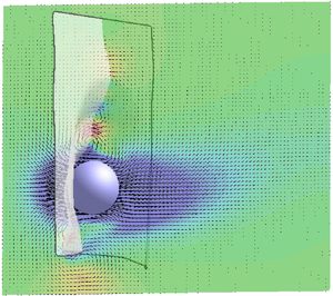
From figure 4 we can see that, when the sphere approaches the membrane, the squeezing of the fluid in the gap produces a pressure build-up that deforms the membrane with a curvature of the same sign as the sphere (figure 4a,c). In contrast, for a receding sphere, the gap widens and fluid is sucked towards the stagnation point by a low pressure that bends the membrane with opposite curvature (figure 4b,d).

Figure 4. (a,b) Instantaneous experimental visualisations of the pendulum (a) approaching the membrane and (b) retreating. Here,  $Re=4200$, $\rho _p/\rho _f=8$ and $e/(2R)=0.1$. (c,d) Numerical results of (false) colour contours of the vertical ( $y$) velocity component overlaid with velocity vectors in the symmetry $y$–
$y$– $z$-plane and in the reference frame of the membrane stagnation point (only every other grid point is shown for clarity). The colours range from blue to red for $-0.8 \leqslant u_y \leqslant +0.8$. Here, $Re=20$, $\rho _p/\rho _f=8$ and $e/(2R)=0.05$. The thin solid line is added to evidence the membrane profile in the $y$–
$y$– $z$-plane.
In the reference frame of the membrane stagnation point the flow field in the gap can be assumed axisymmetric and dominated by the meridional velocity component  $u_\phi$ (figure 5a). The gap thickness can be approximated by the relation $h(\phi ) \approx C(1-\epsilon \cos \phi )$ with $C=R'-R$, $\epsilon =s/C$ and $R'$ the local radius of curvature of the membrane. Note that the same expression can be used also to describe the gap for a receding sphere (figure 5b) provided $C=R'+R+h_0$ and $\epsilon = (R'+R)/C$. Following a similar approach as in Zenit & Hunt (Reference Zenit and Hunt1999) a depth integrated equation for the meridional velocity component is derived from which the pressure at any $\phi$ is computed once the pressure at the colatitude $\phi ^{*}$ is known. The complete derivation is given in appendix A, here we report only the result
 \begin{align} \bar{p}(\phi) &= \bar{p}(\phi^{*})\frac{1-\epsilon \cos\phi^{*}}{1-\epsilon \cos\phi}\nonumber\\ &\quad +\frac{R^{2}}{1-\epsilon \cos\phi} \left \{ \frac{\ddot{\epsilon}}{2}[\cos \phi-\cos \phi^{*}] + \frac{\dot \epsilon^{2}}{4} \left [ \frac{\sin^{2} \phi^{*}}{1-\epsilon \cos\phi^{*}}-\frac{\sin^{2} \phi}{1-\epsilon \cos\phi}\right ]\right \}\nonumber\\ &\quad +\frac{12 R^{2} \dot{\epsilon}}{Re C^{2}(1-\epsilon \cos\phi)}[F(\phi^{*})-F(\phi)],\nonumber\\ &\qquad \textrm{with} \quad F(\phi) = \frac{1}{(1+\epsilon)^{2}}\ln \left [\frac{1+\cos \phi}{1-\epsilon \cos\phi}\right ] - \frac{1}{\epsilon(1+\epsilon)}\frac{1}{1-\epsilon \cos\phi}, \end{align}
which is valid for  $h(\phi ) \ll R$ (with $R=0.5$ for the present scaling).

Figure 5. Idealised sketch of the fluid gap between the sphere or radius  $R$ and the deformed membrane of local radius of curvature $R'$; (a) sphere approaching the membrane, (b) receding sphere.
Equation (3.3) gives the distribution of the pressure  $\bar {p}$ mediated across the gap width $h$ as function of the colatitude $\phi$ whose value depends in a complex way on the gap width dynamics through $\epsilon$, $\dot {\epsilon }$ and $\ddot {\epsilon }$. This gives a result that is different from the ‘simple’ lubrication model as will be shown in appendix A in more detail.
In figure 6 we show the pressure distribution on the membrane for the same case as in figure 4(c,d) together with the profile in  $y$–
$y$– $z$-plane for the approaching (figure 6a,c) and receding (figure 6b,d) dynamics. In this case, thanks to the low Reynolds number ( $Re=20$) and the fine spatial resolution of the simulation, it was possible to check the prediction of (3.3) by choosing configurations where the sphere/membrane distance never decreased below $2\varDelta$ and comparing the pressures. It can be seen that the model yields a good representation of the local pressures although it performs better for the approaching phase than for the receding one: a possible reason is that in the latter case the flow is not completely symmetric and does not fulfil all the hypotheses of the model.

Figure 6. False colour contours of pressure distribution on the membrane (a,b) and pressure profiles along its symmetry  $y$–
$y$– $z$-plane (c,d) for the same case as figure 4(c,d) obtained by numerical simulation. The colours range from blue to red for $-20 \leqslant p \leqslant 10$. In panels (c,d), the symbols are the numerical pressure sampled on the membrane surface while the red solid line is the prediction of (3.3).
Once more we wish to stress that when the sphere approaches the membrane the fluid is squeezed out of the gap owing to the pressure build up and the interaction results in a repulsive force. In contrast, in the receding phase, the fluid is sucked into the gap and the pressure decreases locally thus producing an attractive force between the bodies; this clearly shows that, for the problem of collision in a fluid, all the models based on purely repulsive forces are not physically consistent since they miss the change of sign of the interaction.
The inversion of the fluid displacement in the gap, before and after the impact, has been verified also experimentally as shown in figure 7. In order to make the measurement easier, we have considered the interaction of the pendulum with a rigid (glass) surface and sampled the velocity at a fixed point with a small offset with respect to the symmetry axis (point  $A$ of figure 7a). It is interesting to note that, despite the relatively high frame rate ( $5000$ f.p.s.), the velocity inversion still occurs within one time step ( $200\ \mathrm {\mu } \textrm {s}$) across the instant of impact.

Figure 7. (a) Experimental PIV measurement of the pendulum interaction with a solid (glass) boundary for a case at  $Re=1000$ and $\rho _p/\rho _f=8$. The view is from the side. (b) Time evolution of the $y$ velocity component at point $A$ next to the boundary.
The results of figure 6 were used to show the good agreement of the model of (3.3) with the numerical simulation at  $Re=20$ when the spatial resolution was high enough to capture the dynamics of the first sphere/membrane interaction. A similar quality of agreement is found also for higher Reynolds numbers and figure 8(a) reports the result at $Re=100$ obtained in the same way as the profiles of figure 6.

Figure 8. Pressure profiles along its symmetry  $y$–
$y$– $z$-plane for a case at $Re=100$, $\rho _p/\rho _f=8$ and $e/(2R)=0.1$; (a) $t=4.4$, (b) $t=4.9$. The symbols are the numerical pressure sampled on the membrane surface while the red solid line is the prediction of (3.3).
The model, however, is really useful when the gap becomes smaller than  $2\varDelta$ and the numerical simulation cannot capture the correct pressure profile. An example is given in figure 8(b) in which it is evident that the computed values and the model deviate significantly in the region around $y=0$ where the gap width is the thinnest and decreases below $2\varDelta$.
Additional evidence is provided in figure 9 showing the pressure at the point  $\phi =0$ as a function of the (minimum) gap width. Clearly, until the gap is thicker than $2\varDelta$, the numerical simulation yields a pressure similar to that of (3.3). However, as $h(0)$ decreases below the threshold, the resolution becomes insufficient and pressure in the gap has to be modelled.

Figure 9. (a) Maximum gap averaged pressure  $\bar {p}(0)$ versus minimum gap width $h(0)$ for the case at $Re=100$, $\rho _p/\rho _f=8$ and $e/(2R)=0.1$. The circles are the results of the numerical simulation while the red solid line is the prediction of (3.3). (b) The same as panel (a) but in log–log scale; the red solid line is the prediction of (3.3), the black line is the relation $\bar {p}(0) \sim h(0)^{-2}$ added for comparison.
As an aside, we note that (3.3), despite the complex dependence on various parameters, still gives  $\bar {p}(0) \sim h(0)^{-2}$, thus the pressure scaling is not different from other available models. Nevertheless, as shown in appendix A, (3.3) is derived from the exact integration of the balance of momentum with a few symmetry hypotheses therefore it gives reliable pressure predictions without the use of any user-defined parameter.
On the other hand, the use of (3.3) is very delicate and its prediction is quite sensitive to numerical errors. More in details, during a simulation, for every time step, the distance of the sphere surface from the membrane along the vertical section in the symmetry  $y$–
$y$– $z$-plane, is evaluated and if a region has a distance smaller than $2\varDelta$ the model is activated by replacing the local pressure forces with those of the model. The point of minimum distance is tagged as $\phi =0$ and the local radius of curvature of the membrane is estimated. The first point where the gap is $2\varDelta$ yields $\phi ^{*}$ with pressure $\bar {p}(\phi ^{*})$. All the geometrical parameters are easily evaluated and $\dot {\epsilon }$, $\ddot {\epsilon }$ are computed from the relative velocity of the sphere with respect to the membrane stagnation point ( $\phi =0$).
The derivation of the equation (3.3), further details, technicalities and warnings on the application of this model are given in appendix A.
A final modelling component is the force generated by the physical contact of the objects in those cases in which the pressure build up during the approaching is not enough to prevent the impact. An important observation for the present problem is that the membrane, not only deforms but it also flaps about the upper horizontal edge, therefore the contact with the sphere is usually absorbed by large displacements rather than by deformations with intense internal stresses. Nevertheless, the contact forces between the two structures need to be computed to determine their dynamics and we use the discrete version of the impulse theorem. In fact, being that the sphere is rigid and the membrane deformable, if, after one time step  $\varDelta t$, the $i$th Lagrangian marker of the latter has penetrated the pendulum by a distance $ {\delta }$ with a velocity $\dot { \boldsymbol {x}}_i$, it is moved back by $- {\delta }$ and is assigned the velocity of the sphere $\boldsymbol {u}_s$ at that point. The velocity variation in a time $\Delta t$ for a marker of mass $m_i$ entails a force $\boldsymbol {F}^{c}_i = m_i (\boldsymbol {u}_s-\dot { \boldsymbol {x}}_i)/\Delta t$ which is added to the external forces $\boldsymbol {F}_i^{ext}$. Finally, according to Newton's third law of motion, $-\boldsymbol {F}^{c}_i$ is applied at the same point to the surface of the sphere and it contributes to the moment of the resultant about the centre of rotation.
We wish to stress that the real contact between sphere and membrane occurs only when one or more nodes of the latter fall within the volume of the former (i.e. when the distance of a node from the sphere centre is smaller than its radius) and the discrete impulse theorem is applied.
On the other hand, when the membrane/sphere gap decreases below  $2\varDelta$ we use (3.3) to compute the pressure forces even if the pendulum will never physically touch the membrane.
Perhaps (3.3) could be more correctly referred to as ‘proximity model’ and its activation depends also on the grid resolution; the real contact model is instead only the above discrete impulse theorem as it is used only when the physical contact occurs.
4. Results
Looking at the sketch of figure 2 it appears that this problem has a huge parameter space and investigating all the possibilities within a single research project is unfeasible. This is true even after fixing the geometry of the pendulum, the material properties of the membrane and its geometry and for this reason we have chosen to explore only some of the relevant parameters. In particular, we have relied on quick laboratory flow visualisations to get a clue on the main flow features and afterwards performed some series of numerical simulations changing only one parameter at a time.
4.1. Rigid versus deformable surfaces
In order to stress the differences between the collisions with rigid and deformable surfaces, we start by presenting two cases at low and high Reynolds numbers for the same pendulum impacting on a suspended thin rubber membrane ( $e/(2R)=0.1$) and on a solid block ( $e/(2R)=10$) of the same rubber that can elastically deform without net translation. In figure 10 we show the simulations at $Re=1000$ and $\rho _p/\rho _f=8$ yielding an impact Stokes number of $St=Re \rho _p/(9\rho _f) \simeq 890$ which is far beyond the threshold value ( $St_c \approx 10$) for the rebound from a wall (Zenit & Hunt Reference Zenit and Hunt1999; Joseph et al. Reference Joseph, Zenit, Hunt and Rosenwinkel2001). At this Reynolds number, the sphere dynamics is unaffected by the presence of the boundary until the vertical equilibrium position is reached ( $t=4$ in figure 10a,b); after this point, however, the impact with the solid boundary produces a rebound with an impulsive (within a few time steps ( ${\approx } \mathcal {O}(10\text {--}20$)) velocity inversion ( $t=4.2$ in figure 10c). In contrast, the membrane absorbs the pendulum momentum by deforming (figure 10d) and flapping thus delaying the contact up to $t\simeq 4.4$ and showing only a much weaker rebound.

Figure 10. Comparison of the numerical results for the pendulum interaction with a solid block  $e/(2R)=10$ (a,c,e,g) and a membrane $e/(2R)=0.1$ (b,d,f,h) for a case at $Re=1000$ and $\rho _p/\rho _f=8$; (a,b) $t=4.0$, (c,d) $t=4.2$, (e,f) $t=5.0$, (g,h) $t=6.0$. Snapshots in the $y$–
$y$– $z$-plane; the contours represent the $u_z$ velocity component with the colours blue to red for $-1 \leqslant u_z \leqslant 1$. Also the velocity vectors are overlaid and only one in every three grid points are reported for clarity. The insets of the panels (b,d,f,h) show the structures from below.
More quantitative information can be obtained from the time evolution of the sphere centre reported in figure 13(a,b). The impact with the solid block produces multiple rebounds that can be simply quantified by the restitution coefficient, i.e. the ratio of the velocity magnitudes after ( $U_a$) and before ( $U_b$) the impact; in this case we obtain from the numerical simulation $r=U_a/U_b=0.75$– $0.8$ which is slightly smaller than the values reported by Joseph et al. (Reference Joseph, Zenit, Hunt and Rosenwinkel2001) for glass or other rigid materials but consistent with the fact that the rubber block deforms locally and absorbs some energy.
The interaction with the membrane shows a completely different behaviour that involves the fluid on both sides. In fact, the impact of the pendulum induces a localised jet on the other side of the structure in the same direction as the sphere wake (figure 10f,h). The negative  $z$-velocity of the flow drags the membrane to the left and in turn the sphere thus preventing its translation in the positive $z$ direction.
The reliability of these numerical results has been verified by comparing some quantities with the analogous counterparts measured in a dynamically similar experiment. In figure 11 we report the deformed configuration of lower edge of the membrane at different phases of the collision showing satisfactory agreement.

Figure 11. (a) Experimental visualisation of the pendulum interaction with a membrane  $e/(2R)=0.1$ for a case at $Re=1000$ and $\rho _p/\rho _f=8$. The view is from below as for the insets of figure 10. The membrane lower edge is highlighted by a red solid line. (b) Comparison of numerical (symbols) and experimental (lines) lower edge deformation of the membrane at different times: black, $t=4$; red, $t=5$; blue, $t=6$; orange, $t=7$; green, $t=8$; magenta, $t=9$; yellow, $t=10$; cyan, $t=11$. The profiles are shifted in the $z$-direction by $0.5$ for every time unit for clarity.
Figure 12 shows the time evolution of the pendulum centroid determined by fitting a circumference to the contour of the sphere identified by digitally thresholding the image: it agrees reasonably well with the numerical simulation and this gives us confidence on the validity of the computer simulations. This is a very useful indication as  $Re\approx 1000$ is a sort of ‘overlapping region’ of numerics and experiments since the former cannot be run beyond that threshold because of computational cost while the latter do not access easily the low Reynolds number regime.

Figure 12. (a) Experimental visualisation of the pendulum interaction with a membrane  $e/(2R)=0.1$ for a case at $Re=1000$ and $\rho _p/\rho _f=8$. The view is from the side as for figure 10. The pendulum boundary is highlighted by a red solid line and its centre by a red circle. (b) Comparison of numerical (symbols) and experimental (line) time evolution of the $z$-coordinate of the pendulum centre.
Accordingly, the flow at  $Re=10$ has been investigated only numerically and the results, shown in figure 13(c,d), are very different from those at $Re=1000$. The impact with the solid block shows no rebound and, with $St\simeq 9$, this is consistent with the findings of Joseph et al. (Reference Joseph, Zenit, Hunt and Rosenwinkel2001) who obtained a similar result regardless of the materials of the sphere and the wall. Also the interaction with the membrane is different from that of figure 10 since the dynamics is dominated by viscosity and the momentum of the pendulum is too weak to produce a contact with the structure (see figure 14c). Nevertheless, the membrane deformation causes the sphere to overshoot its equilibrium position until the pressure build up induces a smooth velocity transition from negative to positive values without oscillations.

Figure 13. Time evolution of the pendulum centre  $z$-coordinate (a) and $z$-velocity (b) for the same cases as figure 10: numerical results. Solid line show the impact with a solid block, red dashed line show the interaction with the membrane. (c,d) The same as (a,b) except for $Re=10$.

Figure 14. Time evolution of the pendulum centre  $z$-coordinate (a) and $z$-velocity (b) for a membrane of thickness $e/(2R)=0.1$, a pendulum with $\rho _p/\rho _f=8$ and $Re=10$ (black solid line), $Re=20$ (red dashed) and $Re=100$ (blue dotted). (c) Detail of the configuration at $Re=10$ at the instant of minimum distance (black bullet of panel (b)). (d) The same as panel (c) but for $Re=20$ at the point of velocity inversion (red bullet of panel (b)), (e) the same as panel (c) but for $Re=20$ at the instant of minimum distance (filled red square of panel (b)). The colour map represents the numerical $u_z$ velocity component with the colours blue to red for $-0.1 \leqslant u_z \leqslant 0.1$. Also the velocity vectors are overlaid and only one in every two grid points are reported for clarity.
4.2. Reynolds number effect
Evidently, the interaction dynamics is strongly dependent on the flow Reynolds number and for this reason we have performed a series of numerical simulations and experiments in which this parameter has been varied in the range  $10 \leqslant Re \leqslant 4200$. We have already seen that at the lowest end of $Re$ the flow is viscosity dominated and that at the point of velocity inversion (figure 14b), which is also of minimum distance, there is no contact (figure 14c).
The transition occurs at  $Re=20$ ( $St\simeq 18$) when the pendulum velocity oscillates between positive and negative values because of the dynamic interaction with the membrane (figure 14b). Although at the first velocity inversion sphere and membrane do not touch (figure 14d) the successive flapping of the membrane and residual flow motion causes an incipient contact (figure 14e).
For this configuration we have performed seven numerical simulations in the range  $20 \leqslant Re \leqslant 1000$ and approximately twenty experimental runs for $100 \leqslant Re \leqslant 4200$. The main observations are that for Reynolds numbers bigger than $20$ the contact always occurs already at the first approach and, as shown in figure 14(a,b), already for $Re \geqslant 100$ the collision dynamics becomes similar to that at $Re=1000$ of figure 13 thus showing weak dependence on the Reynolds number. The latter finding has been confirmed up to $Re=4200$ by laboratory experiments.
In the previous analysis we have varied the momentum of the pendulum by changing the Reynolds number; a more effective way, however, is to act on the density of the swinging mass that proportionally changes the impact Stokes number  $St=Re \rho _p/(9\rho _f)$. In the laboratory experiments, using spheres of steel, aluminium and glass, we have qualitatively verified that, for a given membrane, if the Stokes number is the same, the collision dynamics looks similar. Our experimental apparatus, however, cannot access the lowest Reynolds (or Stokes) number regime, therefore we have used the numerical simulation to verify the previous condition for the occurrence of the contact.
In a first simulation we have decreased the Reynolds number to  $Re=10$ but used a ratio $\rho _p/\rho _f=16$ (tantalum/water) while in another the combination it was $Re=40$ and $\rho _p/\rho _f=4$ (titanium/water). Finally, a third simulation at $Re=50$ and $\rho _p/\rho _f=2.7$ (aluminium/water) has been performed and all the results compared with the reference case at $Re=20$ and $\rho _p/\rho _f=8$. The results of figure 15 confirm that, apart from minor differences, the overall dynamics is very similar and all the configurations (not shown here in the sake of brevity) show the incipient contact as for the reference case.

Figure 15. Numerical results for the time evolution of the pendulum centre  $z$-coordinate (a) and $z$-velocity (b) for a membrane with $e/(2R)=0.1$: $\rho _p/\rho _f=8$. Solid line for $Re=20$ and $\rho _p/\rho _f=8$; red dashed, $Re=10$ and $\rho _p/\rho _f=16$; blue dotted, $Re=40$ and $\rho _p/\rho _f=4$; and green chain-dotted, $Re=50$ and $\rho _p/\rho _f=2.7$.
4.3. Effect of membrane thickness
All the results of the previous sections have been obtained for a fixed membrane thickness  $e/(2R)=0.1$ although this parameter must be relevant for the dynamics since the bending stiffness (or flexural rigidity) of a thin structure is $B = Ee^{3}/[12(1-\nu _P^{2})]$ and the above thickness can give a high enough $B$ for the membrane to exhibit a plate behaviour.
For a Poisson ratio  $\nu _P = 0.4$ and a membrane thickness $e/(2R)=0.1$ it results $B/E= 0.0012$ while, when $e$ is halved, the ratio $B/E$ decreases by a factor eight.
Indeed, in figure 16, the experimental flow visualisation at  $Re=4200$, ${\rho _p/\rho _f=8}$ for a membrane of thickness $e/(2R)=0.05$ is reported at four instants of the interaction, showing a quite different dynamics from that of figure 4(a,b). As expected, the thinner membrane develops larger displacements and deformations that propagate through all the structure.

Figure 16. Experimental flow visualisations of the impact of a pendulum at  $Re=4200$, $\rho _p/\rho _f=8$ end $e/(2R)=0.05$: (a) $t=4.5$; (b) $t=6$; (c) $t=8$; and (d) $t=10.5$.
Even if numerical simulations cannot afford this high Reynolds number regime, some cases have been computed at  $Re=50$, showing a consistent dynamics. In particular, as shown in figures 17 and 18, the thinnest membrane ( $e/(2R)=0.03$) does not oppose enough reaction to the pendulum to reverse its swing and the simulation stopped at $t=8$ since the membrane reached the left boundary of the computational domain. Another noticeable effect of the reduced membrane thickness is that a physical contact with the sphere never occurs despite the value of the impact Stokes number of $St \simeq 45$. The contact instead is obtained for $e/(2R)=0.05$ although at later times with respect to the $e/(2R)=0.1$ case and with larger deformations of the membrane.

Figure 17. Numerical results for the configuration at the point of minimum sphere/membrane distance: (a)  $e/(2R)=0.03$, $t=7.8$; (b) $e/(2R)=0.05$, $t=7.4$; (c) $e/(2R)=0.1$, $t=4.5$; and (d) $e/(2R)=0.15$, $t=4.5$. Instantaneous snapshots in the $y$–
$y$– $z$-plane: the contours represent the $u_z$ velocity component with the colours blue to red for $-0.4 \leqslant u_z \leqslant 0.4$. Also the velocity vectors are overlaid and only one in every three grid points are reported for clarity.

Figure 18. Numerical results for the time evolution of the pendulum centre  $z$-coordinate (a) and $z$-velocity (b) at $Re=50$ and $\rho _p/\rho _f=8$. Solid line for $e/(2R)=0.1$, (red dashed $e/(2R)=0.15$, blue dotted $e/(2R)=0.05$), (green chain-dotted $e/(2R)=0.03$).
On the other hand, for a thicker membrane ( $e/(2R)=0.15$) the behaviour is not very different from the reference case except for a slightly stronger sphere rebound. This result is consistent with the cubic dependence of the bending stiffness on the membrane thickness; in fact, as $e/(2R)$ increases, the membrane tends to behave like a plate and, as shown by Sondergaard, Chaney & Brennen (Reference Sondergaard, Chaney and Brennen1990), the restitution coefficient of the impact increases as well thus yielding a stronger rebound.
It is worthwhile also to note that the smaller the bending stiffness of the membrane the more it tends to wrinkle during the deformation and this makes less accurate the contact model of these simulations that eventually becomes unusable. In fact, we have found that for decreasing  $e/(2R)$ also the time step of the simulations needed to be refined and we have not been able to complete any simulation for $e/(2R) < 0.03$.
4.4. Effect of membrane surface
Before concluding this paper we want to briefly show that the collision dynamics is affected also by the surface extension of the membrane whose dimensions, up to now, have been kept constant as in the experiment ( $b/(2R)=6$ and $d/(2R)=4.5$). For this test we have halved the length of the edges ( $b/(2R)=3$ and $d/(2R)=2.25$) while the thickness has been maintained to $e/(2R)=0.1$. In the sake of conciseness we do not report the flow field, however, from trajectory and velocity of the sphere (figure 19), it is evident that a smaller membrane opposes less resistance to the pendulum whose rebound is delayed in time. This can be explained considering that, when the membrane is pushed by the pendulum, the fluid on the other side exerts its inertia that adds to that of the membrane (added mass effect). A reduced surface displaces a smaller volume of fluid and the pendulum decreases its velocity more gradually. Despite the different timing of the interaction, the incipient contact still occurs at $Re=20$ and $St\simeq 18$, although more simulations would be necessary to confirm these results also for other parameter combinations yielding the same impact Stokes number.

Figure 19. Numerical results for the time evolution of the pendulum centre  $z$-coordinate (a) and $z$-velocity (b) at $Re=20$, $\rho _p/\rho _f=8$ and $e/(2R)=0.1$: solid line for the full-size membrane, red dashed line for the half-size membrane.
5. Closing remarks
Motivated by the contact dynamics of the heart valve leaflets, we have focussed on the collision of a rigid sphere with a deformable membrane in a viscous fluid. Although this problem is incomparably simpler than the original intended application still it has a very rich dynamics and a huge parameter space.
We have resorted to laboratory experiments and numerical simulations to perform a series of runs in which only one governing parameter was varied at a time and its effect investigated. Our findings suggest that, similarly to the sphere impact with a rigid boundary, also in this case the collision dynamics mainly depends on the impact Stokes number  $St=Re \rho _p/(9\rho _f)$ and, for a membrane thickness of $e/(2R)=0.1$ the sphere rebound occurs only for $St \geqslant 18$. This value, however, increases as the membrane becomes thinner and at $e/(2R)=0.05$ the threshold becomes $St\approx 45$.
Concerning the key question, as to whether or not the sphere really touches physically the membrane for interactions with the Stokes number beyond the threshold, we cannot give a definitive answer. In fact, in our experiments, even when reducing the visualisation area, the membrane/sphere distance always decreased below our resolution capability. Similar limitations affected the numerical simulation that has to deal with finite time and spatial resolution in addition to ‘proximity’ and collision models.
On the other hand, (3.3) depends in a complex way on several quantities and the only scaling behaviour that was observed is  $\bar {p}(0) \sim h(0)^{-2}$ (see figure 9b). In this respect the model scales as other collision relations and cannot help solving the collision paradox (Zenit & Hunt Reference Zenit and Hunt1999).
Additional analysis would be needed to explore in a more systematic way the dependence of this critical Stokes number on the membrane properties and this would involve also variables that have not been explored in this study. In fact, we have always used the material properties of the silicon rubber ( $\rho _m = 1040\ \textrm {kg}\ \textrm {m}^{-3}$, $E=1.5$ MPa and $\nu _P = 0.4$) although their values are certainly important for the problem since they determine the celerity and amplitude of the Lamb waves on the membrane.
A hint in this direction already comes from figure 17 in which, evidently, the thinner membranes have a smaller wave velocity and the impact perturbation takes more time to travel along the structure (note that the panels of the figure are sampled at different times) thus implying that the interaction remains more localised. Similar outcomes are expected from the Young's modulus  $E$ and density $\rho _m$ and more analysis would be needed to assess their effect.
Equally relevant is the size of the membrane considering the reflection of the Lamb waves at the boundaries; in this paper we have analysed only one size variation and more work would be needed also in this direction.
A ‘side product’ of this study is a novel collision model for the numerical simulation of deformable structures in a viscous fluid. Although computationally expensive and ‘delicate’ (in the sense of its stability) the model has shown to perform satisfactorily for a wide range of computational parameters. Also in this case, however, more work could be done to extend it to the sphere surface with a tangential velocity component which is the case when the approaching body is rotating about its centre.
Acknowledgements
The authors are grateful to V. Meschini for the simulation of cardiovascular flows of figure 1. M. Di Pirro is acknowledged for having produced the rubber membranes and some flow visualisations. Finally the authors thank F. Viola for several discussions on the computational aspects of the problem.
Funding
This investigation has been performed with support of the Grant 2017A889FP ‘Fluid dynamics of hearts at risk of failure: towards methods for the prediction of disease progressions’ funded by the Italian Ministry of Education and University.
Declaration of interests
The authors report no conflict of interest.
Appendix A. Derivation of the pressure in the gap
We consider in figure 5(a) the gap between the sphere and the membrane parametrised as  $h(\phi ) \approx C(1-\epsilon \cos \phi )$ with $C=R'-R$ and $\epsilon = s/C$. The time variation of the gap $\dot {h} = -C \dot {\epsilon }\cos \phi$ produces a meridional velocity that we assume axisymmetric about the polar axis $u_\phi (\phi ,r)$. This velocity is then averaged across the gap width to obtain
 \begin{equation} \bar{u}(\phi) = \frac{1}{h(\phi)}\int_R^{R+h(\phi)} u_\phi (\phi,r)\,\textrm{d}r. \end{equation}
Assuming that  $R'-R \ll 1$ and $h(\phi ) \ll R$, the fluid volume in the gap between the sphere and the membrane is
 \begin{equation} V(\phi) = 2{\rm \pi} R^{2}\int_0^{\phi} \sin(\varphi)h(\varphi)\,\textrm{d}\varphi= 2{\rm \pi} R^{2} C \left[(1-\cos \phi)+\frac{\epsilon}{4}(\cos 2\phi -1)\right], \end{equation}
and the corresponding area of the fluid boundary
 \begin{equation} A(\phi) = 2{\rm \pi} R h(\phi)\sin\phi. \end{equation}
From the mass (volume) conservation we have  $A(\phi )\bar {u}(\phi ) = - \dot {V}(\phi )$ that, with the above definitions, yields
 \begin{equation} \bar{u}(\phi) = \frac{R}{4}\frac{1-\cos 2\phi}{\sin \phi} \frac{ \dot{\epsilon}}{1-\epsilon \cos \phi} \equiv \frac{R}{2}\frac{\dot{\epsilon}\sin \phi}{1-\epsilon \cos \phi}. \end{equation}
The gap averaged momentum equation for the axisymmetric meridional component in spherical coordinates reads
 \begin{equation} R \frac{\partial h \bar{u}}{\partial t} + \frac{\partial h \bar{u}\ \bar{u}}{\partial \phi} = -\frac{\partial h\bar{p}}{\partial \phi} -R (\tau_R+\tau_{R'}), \end{equation}
with  $\tau _R$ and $\tau _{R'}$ the tangential viscous stresses at the sphere and membrane surfaces, respectively. In the above equation, we can substitute the expression (A4) for $\bar {u}$ and solve for the pressure gradient to obtain
 \begin{equation} \frac{\partial h\bar{p}}{\partial \phi} = - \frac{R^{2} C \ddot{\epsilon}}{2} \sin \phi -\frac{\partial}{\partial \phi} \left ( \frac{R^{2} C }{4} \frac{\dot{\epsilon}^{2} \sin^{2} \phi} {1-\epsilon \cos \phi} \right ) - R (\tau_R+\tau_{R'}). \end{equation}
 For the meridional viscous stresses we further assume that the radial profile of the meridional velocity is parabolic in the gap and that, with  $h\ll R$, this results in $\tau _R\simeq \tau _{R'}$. A parabolic velocity profile with mean $\bar {u}$ between two boundaries at distance $h$ yields
 \begin{equation} \tau_R+\tau_{R'} \simeq 2 \tau_R = \frac{12 R\dot{\epsilon}}{Re C}\frac{\cos \phi (1-\cos \phi)} {\sin \phi (1-\epsilon \cos \phi)^{2}}. \end{equation}
After having integrated the viscous terms we pose
 \begin{equation} F(\phi)=\frac{1}{(1+\epsilon)^{2}}\ln \frac{1+\cos \phi}{1-\epsilon \cos \phi}-\frac{1}{\epsilon (1+\epsilon)} \frac{1}{1-\epsilon \cos \phi}, \end{equation}
so that (A6) can be finally integrated between  $\phi ^{*}$ and the generic $\phi$ to obtain
 \begin{align} \bar{p}(\phi)& = \bar{p}(\phi^{*})\frac{1-\epsilon \cos\phi^{*}}{1-\epsilon \cos\phi} \nonumber\\ &\quad +\frac{R^{2}}{1-\epsilon \cos\phi} \left \{ \frac{\ddot{\epsilon}}{2}[\cos \phi-\cos \phi^{*}] + \frac{\dot{\epsilon}^{2}}{4} \left [ \frac{\sin^{2} \phi^{*}}{1-\epsilon \cos\phi^{*}}-\frac{\sin^{2} \phi}{1-\epsilon \cos\phi}\right ]\right \}\nonumber\\ &\quad +\frac{12 R^{2} \dot{\epsilon}}{Re C^{2}(1-\epsilon \cos\phi)}[F(\phi^{*})-F(\phi)]. \end{align}
We wish to point out that this result relies on several simplifying assumptions that are only approximately verified by the real problem: the most important is the flow symmetry in the gap that, therefore, yields a dependence only on  $\phi$. This is quite verified at low Reynolds numbers and during the approaching phase of the dynamics while deviations are observed during the receding phase (figure 6b,d) or for increasing $Re$. The problem is exacerbated for vanishing membrane thickness since it tends to wrinkle during the motion and further deviates from the symmetry condition.
Evaluating locally angles and distances is very sensitive to numerical errors which reflect in inaccurate pressure values. In the present simulations we have computed all the geometrical parameters of the model relying only on the vertical section of the  $y$–
$y$– $z$ symmetry plane and used the same quantities for each azimuthal section around the polar axis $\phi =0$. The model pressure therefore is axisymmetric even if the instantaneous geometry is not, thus adding to the approximations.
Another important point is that the model (A9) diverges for  $\epsilon \rightarrow 1$ yielding an infinite pressure at the axis $\phi =0$. To prevent the simulation from blowing up, the maximum epsilon is limited to $\epsilon \leqslant 0.99$ that, however, is only an arbitrary value; nevertheless, during a numerical calculation only few points ( ${\approx } 30$) and for a limited duration in time ( ${\approx } 50$ time steps) have to be corrected and, if it happens more frequently it is an indication that either the space or time resolutions are not adequate for the run parameters of that case.
It might be worthwhile to note that, in the derivation of (A9), we have disregarded the presence of the disjoining pressure  $\varPi$ which arises from the attractive interaction of two surfaces at a distance $h$. However, according to the classical theory this pressure can be estimated as $\varPi = H/(6{\rm \pi} h^{3})$, with $H$ the Hamaker constant (in the paper by Dai & Leal (Reference Dai and Leal2008) a more refined formula including the surface curvature is given). An estimate of the Hamaker constant for water/silica interfaces (Valmacco et al. Reference Valmacco, Elzbieciak-Wodka, Besnard, Maroni, Trefalt and Borkovec2016) yields a range $7\times 10^{-23} \leqslant H \leqslant 2.4\times 10^{-21}$ J which implies a gap width of the order of $h \approx 1.7\times 10^{-8}$ m (approximately $8\times 10^{-7}$ sphere diameters) to have $\varPi \approx 1$ Pa. Comparatively, the results of figure 6(c,d) show pressure peaks, from (A9), of thousands of Pascal (tens of non-dimensional units) already for the case of figure 4(c,d) for which the gap never becomes thinner than $2\varDelta$ ( ${\approx }1$ mm). This comparison clearly shows that the disjoining pressure can be safely neglected for this problem.
One of the referees has correctly noted that the wall viscous stresses of (A7) assume a parabolic velocity in the form  $u_\phi (\phi ,r) = [6\bar {u}(\phi )/h(\phi )^{2}] (r-R)[R-r+h(\phi )]$ and this profile does not account for the stretching the membrane. A more correct parametrisation should be $u_\phi (\phi ,r) = [W(\phi )/h(\phi )^{2}] (r-R)[R-r+h(\phi )] + [V(\phi )/h(\phi )](r-R)$ with $V(\phi ) =V_0 \tan (\phi /2)$ the wall velocity for a rimless spherical cap and $W(\phi )$ such that the gap averaged $u_\phi (\phi ,r)$ still gives $\bar {u}(\phi )$.
This new velocity distribution can be used in (A1, A6) to obtain a new solution in the form
 \begin{align} \bar{p}(\phi) &= \bar{p}(\phi^{*})\frac{1-\epsilon \cos\phi^{*}}{1-\epsilon \cos\phi} \nonumber\\ &\quad +\frac{R^{2}}{1-\epsilon \cos\phi} \left \{ \frac{\ddot{ \epsilon}}{2}[\cos \phi-\cos \phi^{*}] + \frac{\dot{\epsilon}^{2}}{4} \left [ \frac{\sin^{2} \phi^{*}}{1-\epsilon \cos\phi^{*}}-\frac{\sin^{2} \phi}{1-\epsilon \cos\phi}\right ]\right \}\nonumber\\ &\quad +\frac{3 R}{Re C^{2}(1-\epsilon \cos\phi)} \left \{ \vphantom{\left (\frac{1+\cos \phi^{*}}{1-\epsilon \cos\phi^{*}}\right )}4R\dot{\epsilon} [F(\phi^{*})-F(\phi)]\right.\nonumber\\ &\quad \left.+\frac{2V_0}{1+\epsilon} \left [ \ln \left (\frac{1+\cos \phi}{1-\epsilon \cos\phi}\right )- \ln \left (\frac{1+\cos \phi^{*}}{1-\epsilon \cos\phi^{*}}\right ) \right ] \right \}. \end{align}
Estimating  $V_0$ entails further hypotheses and here we have assumed that a membrane segment of initial length $\ell = R \sin \phi ^{*}$ is deformed into an arch of length $\ell ' = R\phi ^{*}$ by the sphere that decelerates from the initial impact velocity $\alpha U$ (with $\alpha \leqslant 1$, $U$ being the maximum pendulum velocity used to define the Reynolds number) up to rest in a time interval $\delta t$. This yields $V_0 \approx (\ell '-\ell )/\delta t = \alpha U (\phi ^{*}-\sin \phi ^{*})/[2(1-\cos \phi ^{*})]$ that, using the value $\alpha =1$, gives the result of figure 20. As shown in figure 20, it does not differ appreciably from the prediction of (A9) even if the value $\alpha =1$ is definitely too high since it implies the same impact velocity as if the pendulum were freely swinging without the presence of the membrane and the friction of the surrounding fluid. Finally we wish to point out that the above models are not just a lubrication approximation; in fact within the same assumptions the lubrication equation yields (Pinkus & Sternlicht Reference Pinkus and Sternlicht1961)
 \begin{equation} \bar{p}(\phi) = \bar{p}(\phi^{*}) +\frac{6 R^{2} \dot{\epsilon}}{Re C^{2}\epsilon}\left [ \frac{1}{(1-\epsilon \cos \phi)^{2}}- \frac{1}{(1-\epsilon \cos \phi^{*})^{2}}\right ], \end{equation}
which completely misses the contributions of unsteady and convective terms.

Figure 20. Pressure profiles along the symmetry  $y$–
$y$– $z$-plane of the membrane for a case at $Re=20$, $\rho _p/\rho _f=8$ and $e/(2R)=0.1$ (the same case as in figure 6c). The symbols are the numerical pressure sampled on the membrane surface, the red line the prediction of (A9), the blue line the prediction of (A10) while the green line is the result of the lubrication model of (A11).
The pressure distribution predicted by the lubrication model is also shown in figure 20 (green line) and it is interesting to note that, despite the simpler approximation, it captures in a reasonable way the shape of the pressure distribution and overestimates the peak pressure only by slightly more than  $25\,\%$. On the other hand, using (A11) is easier than (A9) or (A10) since the first has a simpler form and does not need $\ddot {\epsilon }$ that is difficult to evaluate and very sensitive to numerical errors.


 Open access