


1. Introduction
Tactical fighters developed since the 1960s predominately feature fuselage-embedded twin-jet engines. Additionally, multi-tube nozzles have been investigated as possible jet noise suppressors, and designs of future distributed-propulsion systems involve placing two or more parallel jet streams in close proximity. The closely spaced jets can interact both at the hydrodynamic and acoustic levels, giving rise to complex flow structures when compared with single round jets at equivalent operating conditions.
Following the seminal works of Mollo-Christensen (Reference Mollo-Christensen1967), the relation between the dominant components of the far-field noise radiated by high-speed jets and large-scale fluctuations in the turbulent mixing region, coherent over several nozzle diameters, has been the subject of growing research (Jordan & Colonius Reference Jordan and Colonius2013; Cavalieri, Jordan & Lesshafft Reference Cavalieri, Jordan and Lesshafft2019). Radiated sound is correlated with large-scale, low-frequency fluctuations in the mixing region and with very few azimuthal modes for single isolated jets (Juvé, Sunyach & Compte-Bellot Reference Juvé, Sunyach and Compte-Bellot1980; Hileman et al. Reference Hileman, Thurow, Caraballo and Samimy2005; Cavalieri et al. Reference Cavalieri, Daviller, Comte, Jordan, Tadmor and Gervais2011). The existence of coherent structures in turbulent jets was first identified by Crow & Champagne (Reference Crow and Champagne1971) and their resemblance to instability waves for harmonically forced supersonic jets suggested the use of linear instability analysis to model them (Crighton & Gaster Reference Crighton and Gaster1976; Michalke Reference Michalke1984). The presence of wavepackets in high-speed jets was finally demonstrated over the last two decades, as well as the ability of linear stability calculations to model them faithfully (Suzuki & Colonius Reference Suzuki and Colonius2006; Gudmundsson & Colonius Reference Gudmundsson and Colonius2011; Cavalieri et al. Reference Cavalieri, Rodríguez, Jordan, Colonius and Gervais2013; Sinha et al. Reference Sinha, Rodríguez, Brès and Colonius2014). The success of linear stability analysis in predicting the large-scale turbulent fluctuations is attributed to the observation that most nonlinearities are already introduced in the establishment of the mean flow, and that in the natural turbulent jet the different modes are, to some extent, allowed to coexist and develop independently (Schmidt et al. Reference Schmidt, Towne, Rigas, Colonius and Brès2018).
As opposed to single round jets, instability analyses for twin jets are scarce in the literature, due to the mathematical complexity of the latter. The mean turbulent flow corresponding to isolated round jets is axially symmetric, enabling the introduction of azimuthal Fourier modes (each one characterised by an integer wavenumber  $m$) and only requires spatial discretisation in the radial direction. Bipolar coordinates were used by Morris (Reference Morris1990) to study the inviscid instability of two axially homogeneous parallel jets. He identified the counterparts of the different azimuthal Fourier modes known for single jets and classified them according to the symmetries about the jet-centre plane and the plane normal to it. Green & Crighton (Reference Green and Crighton1997) used a similar approach to study coupled oscillation modes of the jet cores, considering varicose and sinuous flapping motions of the two jets. More recently, Rodríguez, Jotkar & Gennaro (Reference Rodríguez, Jotkar and Gennaro2018) and Nogueira & Edgington-Mitchell (Reference Nogueira and Edgington-Mitchell2021) analysed the local linear instability of twin-jet configurations by applying two-dimensional cross-stream discretisations that do not restrict the spatial structure of the wavepackets. Interestingly, the latter analyses recover the same families of eigenmodes corresponding to the Fourier modes of single jets, albeit modified on account of the jet–jet interaction; additional eigenmodes corresponding to mechanisms not present for single jets were not identified. The recent conference paper Rodríguez et al. (Reference Rodríguez, Stavropoulos, Nogueira, Edgington-Mitchell and Jordan2022) revisits the parallel-flow instability of twin jets. Four independent discrete eigenmodes appear for each $m$, regardless of whether the symmetry/anti-symmetry conditions are imposed in the computations or not. Each eigenmode satisfies naturally one of the possible combinations of symmetry/anti-symmetry conditions. It is observed that the eigenfunctions for $m > 0$ modes do not correspond to helical oscillations, but constitute combinations of the respective $+m$ and $-m$ helical modes with the precise phase relationship such that they describe flapping motions on the lateral or vertical planes.
This is consistent with experimental observations and simulations in supersonic twin round jets. Seiner, Manning & Ponton (Reference Seiner, Manning and Ponton1988) and Wlezien (Reference Wlezien1989) showed that the B-mode of oscillation associated with screech manifests as a coupled flapping motion of the plumes occurring in the plane containing the jets. Alkislar et al. (Reference Alkislar, Krothapalli, Choutapalli and Lourenco2005) reported that the coupling between the two jets, for their particular conditions of jet Mach number  $M_j$ and jet separation $s$, results in a symmetric flapping with respect to the mid-plane and dominant jet oscillations occurring in the plane containing the jets (referred to as lateral flapping). A similar observation was made by Gao, Xu & Li (Reference Gao, Xu and Li2016) based on large eddy simulations. The experiments by Kuo, Cluts & Samimy (Reference Kuo, Cluts and Samimy2017) considered a twin-jet configuration with separation $s/D = 2$ and convergent–divergent nozzles with a design Mach number of 1.23 and jet Mach numbers between $M_j = 1.15$ and 1.4. The jets exhibited coupled oscillations, with a varicose (symmetric) lateral flapping motion being observed at conditions in which a single jet would present the helical oscillations typical of the screech B-modes. Experiments undertaken by Knast et al. (Reference Knast, Bell, Wong, Leb, Soria, Honnery and Edgington-Mitchell2018) and Bell et al. (Reference Bell, Soria, Honnery and Edgington-Mitchell2018) reported both helical and flapping oscillations in twin jets, but due to experimental constraints, the presence or absence of helical modes could not be rigorously determined. Later, Bell et al. (Reference Bell, Cluts, Samimy, Soria and Edgington-Mitchell2021) demonstrated that, even at a fixed operation condition, twin-jet oscillations present intermittency. At some time lapses the motion of the two jets can be uncorrelated and present helical motions; at other lapses they are strongly correlated and present a coupled lateral flapping.
This paper revisits the locally parallel linear instability of twin-jet configurations. The first objective is to demonstrate that the coupling of the two jets favours flapping motions over helical ones. The analysis is focused on  $m=1$ modes, as experiments show their prevalence over other modes for most flow conditions in the supersonic regime, especially in the first diameters from the nozzle lip. The second objective is to map the preferred flapping mode for each Strouhal number and jet separation, and the impact of the jet Mach number and temperature ratio upon them. Two independent formulations of the linearised equations are used: (i) an approach that discretises the cross-stream plane using Cartesian coordinates, valid for of finite-thickness jets of arbitrary shape; and (ii) an inviscid vortex-sheet method analogous to that used by Morris (Reference Morris1990), Du (Reference Du1993) and Stavropoulos et al. (Reference Stavropoulos, Mancinelli, Jordan, Jaunet, Weightman, Edgington-Mitchell and Nogueira2023). Section 2 describes the two formulations. Section 3 presents the results of the analyses. The relevant eigenmode families are described briefly. The impact of the interaction of the pressure fields of the two jets on the eigenmodes and the appearance of preferred modes is then discussed. A parametric study is then presented that analyses the effect of the jet Mach number and temperature ratio on the preferred oscillation mode. The main conclusions are summarised in § 4.
2. Formulations of the linear stability problem for twin jets
The twin-jet geometry and geometrical parameters are shown in figure 1. The nozzle diameter is  $D$ and the separation between the jet axes is $s$. The streamwise coordinate $x$ is oriented perpendicular to the paper towards the reader. Radial and azimuthal coordinates measured from the origin are denoted by $(r,\theta )$, and those measured with respect to the axis of each jet are denoted by $(r_1,\theta _1)$ and $(r_2,\theta _2)$. Physical quantities are made dimensionless using $D$ and the free-stream sound speed $c_\infty$ and density $\rho _\infty$. Pressure is scaled with $\rho _\infty c^2 _\infty$ and temperature with $(\gamma -1)T_\infty$, where $\gamma$ is the ratio of specific heats. The jet acoustic Mach number is defined as $M_j = U_j / c_\infty$, with $U_j$ being the jet exit velocity. The jet temperature ratio is defined as $T_R = T_j / T_\infty$, where $T_j$ is the jet exit temperature and $T_\infty$ the free-stream temperature.

Figure 1. Twin-jet configuration and geometry, showing the different coordinate systems employed.
Let  $\boldsymbol {q}'$ be a vector containing all the fluid variables of interest, e.g. the velocity $\boldsymbol {v}=(u,v,w)$, density $\rho$, pressure $p$ and temperature $T$. Linear stability theory (LST) studies small-amplitude disturbances superimposed on a time-invariant flow, either steady laminar or stationary turbulent mean flow, denoted here by $\bar {\boldsymbol {q}}$. Invoking the locally parallel-flow assumption, modal disturbances of the form
 \begin{equation} \boldsymbol{q}'(\boldsymbol{x},t) = \boldsymbol{q}(\kern0.7pt y,z) \exp({\mathrm{i} \left(k x - \omega t\right)}) + \mathrm{c.c.}, \end{equation}
are introduced, where  $\omega$ is the circular frequency, $k$ the streamwise wavenumber, $t$ the dimensionless time and c.c. denotes the complex conjugate. The Strouhal number, defined as $St = f D/U_j$, is related to the dimensionless angular frequency by $\omega = 2 {\rm \pi}M_j St$. The derivation of the LST problem continues by substituting the modal decomposition (2.1) into the linearised governing equations and recasting the result as an eigenvalue problem. The spatial instability framework is used in this work, which consists of prescribing a real frequency $\omega$ and obtaining the corresponding eigensolutions as the eigenvalue/eigenfunction pairs $(k,\boldsymbol {q})$. Thus, LST provides the dispersion relation $\mathcal {D}(\omega,k) = 0$ that governs the evolution of linear instability waves.
The LST is applied here to twin-jet configurations. As opposed to single round jets, axial symmetry cannot be exploited here to simplify the LST problem; however, the twin-jet mean flow is symmetric with respect to the  $(x,y)$- and $(x,z)$-planes. Following Morris (Reference Morris1990), the LST solutions are separated into four families corresponding to the even or odd character of their pressure field with respect to the two planes. The two-letter notation used by Rodríguez et al. (Reference Rodríguez, Jotkar and Gennaro2018) and Nogueira & Edgington-Mitchell (Reference Nogueira and Edgington-Mitchell2021) is adopted to classify the mode families, which is outlined in table 1. Two different formulations of the LST problem are used in this work, as described next.
Table 1. Classification of mode families depending on the symmetries. The fourth column shows the relation of the notation used here to that by Morris (Reference Morris1990). The azimuthal dependence for each family is also shown. The last two columns show the values of  $\phi _y$ and $\phi _z$ appearing in the vortex-sheet model.

2.1. Formulation 1: complete compressible Navier–Stokes equations discretised in Cartesian coordinates
This formulation is valid for finite-thickness jets of arbitrary shape and has been applied previously to twin round jets (Rodríguez et al. Reference Rodríguez, Jotkar and Gennaro2018; Rodríguez Reference Rodríguez2021) and rectangular jets (Rodríguez, Prasad & Gaitonde Reference Rodríguez, Prasad and Gaitonde2021). In these works, the results of the locally parallel LST were used as initial conditions for the subsequent integration of the plane-marching parabolised stability equations. The viscous compressible continuity, momentum and energy equations in Cartesian coordinates are used as the departure point. Ideal gas is assumed and the impact of temperature on viscosity is neglected. In the linearisation, density and temperature are used for the mean flow and pressure and temperature for the disturbances. The modal form (2.1) is introduced and the resulting generalised eigenvalue problem is recast in the form
 \begin{equation} \boldsymbol{\mathsf{L}} \boldsymbol{q} = k \boldsymbol{\mathsf{R}} \boldsymbol{q}, \end{equation}
where matrix operators  $\boldsymbol{\mathsf{L}}$ and $\boldsymbol{\mathsf{R}}$ depend on the mean flow and its derivatives, $\omega$, the physical parameters $Re$,
$Re$,  $Ma$,
$Ma$,  $Pr$ and $\gamma$ (Reynolds, Mach and Prandtl numbers and ratio of specific heats, respectively) and parameters describing the twin-jet configuration (e.g. $s/D$, $M_j$, $T_R$).
The rectangular domain  $\varOmega = [0,y_{\infty }]\times [0,z_{\infty }]$ is used in the discretisation. An analytical coordinate transformation is applied independently to the $y$ and $z$ coordinates to concentrate points around the jet shear layer. The odd/even behaviours of each family are imposed as boundary conditions along the $y = 0$ and $z = 0$ axes. For modes that are respectively symmetric (S) and anti-symmetric (A) with respect to the $(x,y)$-plane, the conditions
 $$\begin{gather} \mbox{S}: \ \dfrac{\partial p}{\partial y} = \dfrac{\partial T}{\partial y} = \dfrac{\partial u}{\partial y} = \dfrac{\partial v}{\partial y} = 0, \quad w = 0, \end{gather}$$
 $$\begin{gather}\mbox{A}: \ p = T = u = v = 0, \quad \dfrac{\partial w}{\partial y} = 0, \end{gather}$$
are imposed at  $y=0$, and similarly for the behaviour with respect to the $(x,z)$-plane. Vanishing of the disturbance velocity and temperature is imposed as far-field boundary conditions. A Neumann condition is imposed for the pressure. The rectangular domain $\varOmega =[0,7.5]\times [0,5]$ was checked to be large enough for the convergence of the results for the case with the largest jet separation considered herein ( $s/D = 5$), and is used for all calculations.
The linear operators  $\boldsymbol{\mathsf{L}}$ and $\boldsymbol{\mathsf{R}}$ are discretised using a combination of variable-stencil high-order finite differences and sparse algebra that exploits the banded structure of the differentiation matrices. A 7-point stencil is used, which results in the optimal balance between accuracy and computational cost (Gennaro et al. Reference Gennaro, Rodríguez, Medeiros and Theofilis2013; Rodríguez & Gennaro Reference Rodríguez and Gennaro2017). After discretisation of the linear operators, the matrix eigenvalue problem (2.2) is solved using an in-house sparse implementation of the shift-and-invert Arnoldi algorithm (Arnoldi Reference Arnoldi1951). Arnoldi's algorithm requires the solution of a number of linear problems, which is accomplished using the package MUMPS (Amestoy et al. Reference Amestoy, Duff, L'Excellent and Koster2001).
This formulation can also be applied without exploiting/imposing the symmetries, as done in Rodríguez et al. (Reference Rodríguez, Jotkar and Gennaro2018). In this case, the computational domain used is  $\varOmega = [-y_{\infty },y_{\infty }]\times [-z_{\infty },z_{\infty }]$ and the same mode families are recovered. The results of the present formulation have been cross-validated with the formulation presented by Nogueira & Edgington-Mitchell (Reference Nogueira and Edgington-Mitchell2021), that employs a Floquet formalism on the azimuthal direction to reduce the computation to a sector of the azimuthal domain and discretises it using a two-dimensional mesh in polar coordinates.
2.2. Formulation 2: vortex-sheet formulation for twin jets
The vortex-sheet model treats the shear layer as a boundary of infinitesimal width with a uniform streamwise velocity inside the jet and zero streamwise velocity outside (Lessen, Fox & Zien Reference Lessen, Fox and Zien1965; Michalke Reference Michalke1970). The inviscid equations governing the linear instability waves, upon the introduction of the modal form (2.1) written in terms of the cylindrical coordinates, reduce to the Helmholtz equation for the disturbance pressure  $p$
$p$
 \begin{equation} \dfrac{\partial^2 p}{\partial r^2} + \dfrac{1}{r}\dfrac{\partial p}{\partial r} + \dfrac{1}{r^2}\dfrac{\partial^2 p}{\partial \theta^2} - \lambda^2 p = 0. \end{equation}
This equation describes the disturbance pressure in the inner ( $i$) and outer ( $o$) regions to the vortex sheet, depending on the definition of $\lambda$
 \begin{equation} \lambda_{i} = \sqrt{k^2 -\frac{1}{T_R}(\omega-M_{j} k)^2}, \quad \lambda_{o} = \sqrt{k^2 -\omega^2}. \end{equation}
In the twin-jet configuration (Morris Reference Morris1990; Du Reference Du1993; Stavropoulos et al. Reference Stavropoulos, Mancinelli, Jordan, Jaunet, Weightman, Edgington-Mitchell and Nogueira2023), the inner and outer solutions are written in forms consistent with the separation in even/odd families as
 \begin{align} p_{i,1} (r_1,\theta_1) &= \sum ^\infty _{m=0} \hat{A}_m {\rm I}_m(\lambda_i r_1) \cos(m\theta_1) + \hat{B}_m {\rm I}_m(\lambda_i r_1) \sin(m \theta_1), \end{align}
 \begin{align} p_o(r_1,\theta_1,r_2,\theta_2) & = \sum ^\infty _{m=0} A_m \left[ {\rm K}_m(\lambda_o r_1) \cos(m\theta_1) + ({-}1)^m {\rm K}_m(\lambda_o r_2) \cos(m\theta_2)\right] \nonumber\\ &\quad+ \sum ^\infty _{m=0} B_m \left[ {\rm K}_m(\lambda_o r_1) \cos(m\theta_1) - ({-}1)^m {\rm K}_m(\lambda_o r_2) \cos(m\theta_2)\right] \nonumber\\ &\quad + \sum ^\infty _{m=0} C_m \left[ {\rm K}_m(\lambda_o r_1) \sin(m\theta_1) + ({-}1)^m {\rm K}_m(\lambda_o r_2) \sin(m\theta_2)\right] \nonumber\\ &\quad + \sum ^\infty _{m=0} D_m \left[ {\rm K}_m(\lambda_o r_1) \sin(m\theta_1) - ({-}1)^m {\rm K}_m(\lambda_o r_2) \sin(m\theta_2)\right] , \end{align}
where  ${\rm I}_m$ and ${\rm K}_m$ are the modified Bessel functions of first and second kind. Each line of (2.8) corresponds to one of the four families.
The inner and outer solutions are matched at the ideally expanded diameter  $D_j$, that is imposed to be equal to $D$ in this work. Matching conditions impose the continuity of the pressure and displacement across the vortex sheet
 $$\begin{gather} p_i(\lambda_i D_j / 2) = p_o (\lambda_o D_j / 2), \end{gather}$$
 $$\begin{gather}\left. \dfrac{\partial p_i}{\partial r} \right|_{r=D_j/2} = \dfrac{1}{T_R}\dfrac{(\omega - kM_j)^2}{\omega^2}\left. \dfrac{\partial p_o}{\partial r} \right|_{r=D_j/2}. \end{gather}$$
In order to impose the matching conditions, the outer solution (2.8) is re-written in terms of the coordinates of a single jet using Graf's addition theorem (Abramowitz & Stegun Reference Abramowitz and Stegun1964)
 $$\begin{gather} {\rm K}_m (\lambda_o r_2) \cos(m\theta_2) = \sum ^{\infty}_{n ={-}\infty} ({-}1)^n {\rm K}_{m-n} (\lambda_o s){\rm I}_n(\lambda_o r_1) \cos(n \theta_1), \end{gather}$$
 $$\begin{gather}{\rm K}_m (\lambda_o r_2) \sin(m\theta_2) = \sum ^{\infty}_{n ={-}\infty} ({-}1)^n {\rm K}_{m-n} (\lambda_o s){\rm I}_n(\lambda_o r_1) \sin(n \theta_1). \end{gather}$$
Combining (2.7)–(2.12) and collecting terms corresponding to the same family yields the dispersion relation for a twin-jet system as
 \begin{equation} \mathcal{D}(\omega,k;M_j,s/D,D_j) = \sum_{m=0}^{\infty}\psi_{m}[a_{nn}\delta_{mn} + \phi_y ({-}1)^m c_{mn}] = 0, \end{equation}
where  $\psi _m$ correspond to the coefficients $A_m, B_m, C_m$ or $D_m$ depending on the solution family, $\delta _{mn}$ is the Kronecker delta and
 \begin{align} a_{nn} &= \frac{1}{\left(1-\dfrac{kM_{j}}{\omega}\right)^2}-\frac{1}{T_R}\frac{\lambda_o}{\lambda_i}\frac{{\rm K}_n^{\prime}\left(\dfrac{D_{j}\lambda_o}{2}\right) {\rm I}_n\left(\dfrac{D_{j}\lambda_i}{2}\right)}{{\rm I}_n^{\prime}\left(\dfrac{D_{j}\lambda_i}{2}\right){\rm K}_n\left(\dfrac{D_{j}\lambda_o}{2}\right)}, \end{align}
 \begin{align} c_{mn} & = ({-}1)^n\epsilon_n[{\rm K}_{m-n}(\lambda_o s) + \phi_z {\rm K}_{m+n}(\lambda_0s)] \nonumber\\ &\quad \times \left[\frac{{\rm I}_n\left(\dfrac{D_{j}\lambda_o}{2}\right)}{{\rm K}_n\left(\dfrac{D_{j}\lambda_0}{2}\right)}\frac{1}{\left(1-\dfrac{kM_{j}}{\omega}\right)^2}- \dfrac{1}{T_R}\dfrac{\lambda_o}{\lambda_i}\dfrac{{\rm I}_n\left(\dfrac{D_{j}\lambda_i}{2}\right){\rm I}_n^{\prime}\left(\dfrac{D_{j}\lambda_o}{2}\right)}{{\rm K}_n\left(\dfrac{D_{j}\lambda_o}{2}\right){\rm I}_n^{\prime}\left(\dfrac{D_{j}\lambda_i}{2}\right)}\right]. \end{align}
Here,  $\epsilon _{n}$ is equal to 0.5 if $n$ = 0 and 1 otherwise. The mode families are imposed through the factors $\phi _y$ and $\phi _z$ in (2.13) and (2.15) (see table 1). For large $s$, the first factor in brackets in (2.15) tends to zero, leaving only those from (2.14), which recovers the dispersion relation for a single jet (Lessen et al. Reference Lessen, Fox and Zien1965; Towne et al. Reference Towne, Cavalieri, Jordan, Colonius, Schmidt, Jaunet and Brès2017). As opposed to the case of a single jet, (2.13) couples all the azimuthal $m$ numbers. For the practical solution, the summatory is truncated at a finite $N$. The results presented in this work are computed using $N = 5$, but their convergence has been checked with a maximum $N$ of 10.
3. Results
3.1. Finite-thickness single- and twin-jet mean flows
The calculations of finite-thickness single and twin jets in this work employ analytic mean flows for the sake of reproducibility. The analytical velocity profile proposed by Michalke (Reference Michalke1970, Reference Michalke1984) is used
 \begin{equation} \frac{\bar{u}}{U_j} = \dfrac{1}{2} \left[ 1 + \tanh\left( \frac{1}{4}\frac{R}{\theta} \left(\frac{R}{r} - \frac{r}{R} \right) \right) \right], \end{equation}
where  $r$ is the radial coordinate measured from the jet centre for a single jet and $R$ is the nozzle radius, $R = D/2$. A tailored mean flow field is constructed for twin-jet configurations by combining the flow fields corresponding to two isolated round jets of the form (3.1) aligned with the $x$-direction and with the centres placed symmetrically at the coordinates $(\kern0.7pt y,z)=(\pm s/2,0)$, as shown in figure 1. This is a good approximation of the twin-jet mean flow in the region immediate downstream of the nozzles, known as the converging region (Okamoto et al. Reference Okamoto, Yagita, Watanabe and Kawamura1985; Moustafa Reference Moustafa1994), where the shear layers of the two jets are still well separated, and has been used in the past in the linear stability calculations by Morris (Reference Morris1990), Rodríguez et al. (Reference Rodríguez, Jotkar and Gennaro2018) and Rodríguez (Reference Rodríguez2021). Recently, Stavropoulos et al. (Reference Stavropoulos, Mancinelli, Jordan, Jaunet, Weightman, Edgington-Mitchell and Nogueira2023) and Padilla-Montero et al. (Reference Padilla-Montero, Rodríguez, Jaunet, Girard, Eysseric and Jordan2023) further assessed the validity of the tailored mean flow by comparison with experimental measurements and numerical simulations of the actual twin-jet geometry, showing it to be a valid approximation at least for the first $\sim$5 diameters of evolution for jets in close proximity.
A zero mean pressure gradient is assumed and the Crocco–Busemann relation particularised for the temperature ratio  $T_R$
$T_R$
 \begin{equation} \frac{\bar{T}}{T_\infty} = (U_j - \bar{u}) \frac{\bar{u}}{2} + \frac{1}{\gamma -1}\left(1 + (T_R-1)\dfrac{\bar{u}}{U_j} \right), \end{equation}
is used to determine the mean temperature  $\bar {T}$. All the quantities in this expression are dimensionless, as explained in § 2. The mean density field $\bar {\rho }$ is obtained from the state equation. Following the parallel-flow assumption, cross-stream mean velocity components are neglected. For the finite-thickness calculations herein, the jet Mach number is set at $M_j = 1.5$ and $T_R = 1$ and the parameter $R/\theta = 12.5$, unless stated otherwise. This value of $R/\theta$ is representative of the thin shear layer in the first diameter from the nozzle (Crighton & Gaster Reference Crighton and Gaster1976; Michalke Reference Michalke1984). The parameter $R/\theta$ is varied in § 3.4, that studies the impact of the shear-layer thickness on the stability results. The Reynolds number $Re = 5\times 10^4$ is used in the calculations but identical results are recovered for $Re = 10^5$, showing that the effect of viscosity is negligible.
3.2. The eigenspectra of single and twin jets
This section discusses the results of the LST analysis based on Cartesian coordinates, described in § 2.2, when applied to single and twin jets.
3.2.1. Single round jets
When the local stability analysis is applied to single round jets, the axial symmetry of the mean flow allows for the introduction of azimuthal Fourier modes of the form  $\exp (\mathrm {i} m\theta )$ (e.g. Gill Reference Gill1965; Michalke Reference Michalke1984). This is usually exploited to reduce the eigenvalue problem to a one-dimensional one, dependent on the radial coordinate alone. For each $m$, the stability analysis recovers different families of eigensolutions (Tam & Hu Reference Tam and Hu1989; Rodríguez et al. Reference Rodríguez, Sinha, Brès and Colonius2013), but only one discrete eigenmode is associated with the Kelvin–Helmholtz (K–H) instability.
The present approach is based on Cartesian coordinates, discretising only the first quadrant of the  $(\kern0.7pt y,z)$-plane and imposing symmetric/anti-symmetric conditions at the $y= 0$ and $z= 0$ planes. As a consequence, it does not isolate the individual azimuthal eigenmodes. Conversely, the imposed symmetries separate the eigenmodes into four families: SS, AS, SA and AA, as shown in table 1 and discussed elsewhere (Morris Reference Morris1990; Rodríguez Reference Rodríguez2021; Rodríguez et al. Reference Rodríguez, Prasad and Gaitonde2021). When this approach is applied to a single jet centred at the origin of coordinates, each eigenspectrum contains a number of discrete K–H eigenmodes, each one corresponding to one $m$. Figure 2(a) shows the eigenspectra for a single jet at $St=0.3$. The different symbols correspond to one of the solution families. Except for $m=0$, which is only recovered in family SS, all other eigenvalues appear repeated in two families. In particular, the eigenmodes corresponding to $m=1$ are recovered in families AS and SA; in the following these eigenmodes are referred to as AS1 and SA1, respectively. Their pressure eigenfunctions are shown in figure 3(a,b). The three-dimensional pressure fields are reconstructed following (2.1), with the eigenfunction $p(\kern0.7pt y,z)$ normalised. To aid in the visualisation, an arbitrary streamwise domain of length $10D$ is used and the pressure field amplitude is multiplied by $\exp (-k_i x)$ to cancel the spatial growth, so that the amplitude remains constant. The pressure vanishes simultaneously at one of the coordinate axes (different for SA and AS) for the real and imaginary components. This behaviour is enforced here by the symmetry/anti-symmetry conditions for each family, but a computation using the domain $\varOmega = [-y_{\infty },y_{\infty }]\times [-z_{\infty },z_{\infty }]$ and not imposing the symmetries delivers identical families of eigenfunctions (Rodríguez et al. Reference Rodríguez, Jotkar and Gennaro2018). Figure 3(d,e) shows the phase of the pressure field, $\phi = \arctan ({\rm Im}(p)/{\rm Re}(p))$, extracted at a cylinder of radius 0.75 $D$ aligned with the jet axis. The azimuthal angle $\theta _1$ is measured from the positive $y$ axis as shown in figure 1. Only the subdomain $\theta _1 \in [0,{\rm \pi} ]$ is shown, but the omitted region can be inferred from the symmetries. Mode SA1 presents a constant phase for $-{\rm \pi} /2 < \theta _1 < {\rm \pi}/2$ which is shifted by an angle ${\rm \pi}$ for other values of $\theta _1$. Mode AS1 shows a similar behaviour but with the phase shift at $\theta _1 = {\rm \pi}$. Each of these eigenfunctions describes a jet flapping motion. However, because the eigenvalues corresponding to the modes AS1 and SA1 are identical ( $k_{SA1} = k_{AS1}$), a linear combination of them is also a valid solution to the general problem. With appropriately chosen amplitude coefficients for each eigenmode, their linear combination recovers the features of a helical mode. This is illustrated in figure 3(c,f), in which the pressure fields of modes AS1 and SA1 are added as
 \begin{align} p(x,y,z,t) = \hat{p}_{\mathrm{SA1}} (\kern0.7pt y,z)\exp({\mathrm{i}(k_{\mathrm{SA1}} x - \omega t)}) + \mathrm{i}\,\hat{p}_{\mathrm{AS1}} (\kern0.7pt y,z)\exp({\mathrm{i}(k_{\mathrm{AS1}} x - \omega t) }) + \mathrm{c.c.} \end{align}
The helical nature of the resulting mode is manifest in the linear dependence of the phase  $\phi$ on the azimuthal angle $\theta _1$.

Figure 2. The LST eigenspectra corresponding to  $M_j=1.5, T_R = 1, R/\theta = 12.5$ and $St=0.3$ and the four solution families: SS ( $+$), AS ( $\circ$), SA ( $\times$), AA ( $\square$). (a) Single jet; (b) twin jet with separation $s/D = 2.2$.

Figure 3. Pressure eigenfunctions corresponding to a single jet at  $M_j=1.5, T_R = 1, R/\theta = 12.5$ and $St = 0.3$. The streamwise dependence is obtained from the corresponding eigenvalue, eliminating the spatial growth. (a–c) Iso-contours of the real pressure component. The grey circle shows the nozzle circumference. (d–f) Phase angle $\phi$ at a cylinder of radius 0.75 $D$. (a,d) SA1; (b,e) AS1; (c,f) linear combination of SA1 and AS1 to produce the $m=1$ helical mode.
3.2.2. Twin round jets
For the twin-jet configuration, the jet axes are not located at the origin of coordinates; while the nomenclature used for the single jet remains valid, the four solution families do not separate the odd and even  $m$ modes. Instead, each family contains one eigenmode for each of the $m > 0$ modes. The symmetry of the mean flow about the mid-plane leads to the recovery of the $m=0$ mode only in the SS and SA families. Representative eigenspectra for a twin-jet configuration with separation $s/D = 2.2$ at $St=0.3$ are shown in figure 2(b), to be compared with the single-jet eigenspectra in figure 2(a).
The interaction between the fluctuation fields of the two jets breaks the azimuthal symmetry of the eigenmodes and the same  $m$ mode presents different eigenvalues $k$, one for each symmetry family. This shift of the eigenvalues with respect to the single-jet ones is stronger for $m=0$ and gradually reduces for increasing $m$. This behaviour is explained by the asymptotic decay of the single-jet eigenfunctions as $r\to \infty$, $\boldsymbol {q} \sim r^{-1/2} \exp (-r \sqrt {k^2 - \omega ^2} )$ (Abramowitz & Stegun Reference Abramowitz and Stegun1964). For a fixed frequency $\omega$, the axial wavenumber $k$ increases with increasing $m$, and hence leads to a faster radial decay of the fluctuations. Consequently, the amplitude of the pressure field associated with one jet that reaches the other jet is reduced. For the same reason, the magnitude of the eigenvalue shift is also inversely proportional to the jet separation $s/D$, as shown next.
In what follows, attention is focused on the  $m=1$ modes, which present the largest growth rates for most of the conditions considered. These modes are denoted by SS1, SA1, AS1 and AA1, where the two letters correspond to the symmetry family and the number to the corresponding azimuthal number. Figure 4 shows the eigenvalues corresponding to each of the four families as a function of the jet separation. While the magnitude of the eigenvalue shift grows continuously with decreasing $s/D$, the dependence of the real and imaginary parts of the eigenvalues is non-monotonic and different for each family. The shift is stronger for modes SS1 and SA1, which correspond respectively to in-phase (varicose) and counter-phase (sinuous) lateral flapping oscillations in the plane containing the jet axes. For jet separation above $s/D \approx 2$, the real part of the wavenumber $k$ is reduced (equivalently, the phase velocity is increased) for SA1, while it is increased for SS1. This behaviour is reversed for very small jet separations. The flapping modes in the vertical (perpendicular) plane follow a similar trend: the in-phase mode AS1 reduces its phase velocity resulting from the presence of the other jet and the counter-phase AA1 increases it. As shown in figure 4(c) and more clearly in the zoomed-in version 4(d), the spatial growth rate presents a similar behaviour for the two pairs of modes:
(i) The in-phase flapping modes SS1 (blue) and AS1 (red) exhibit an increase of the growth rate ( $-k_i$) as $s/D$ is reduced from $s/D \rightarrow \infty$, due to jet interactions. For decreasing separations, the growth rate eventually reaches a maximum, then equals that of the single jet and then becomes smaller, i.e. close jet proximity stabilises the in-phase flapping modes. The jet separations for the destabilisation/stabilisation inversion are different for the two modes: $s/D \approx 2.8$ for SS1 and 2.5 for AS1. The variation of the growth rate is of bigger amplitude for the varicose lateral flapping mode SS1.
(ii) The counter-phase modes SA1 (yellow) and AA1 (black) present opposite trends to the in-phase modes. These modes have the largest growth rates for small jet separations and, in particular, mode SA1 corresponding to sinuous lateral flapping is the most amplified one.


Figure 4. Dependence of the  $m=1$ eigenvalues on the jet separation $s/D$: (a) the complex $k$ plane. The eigenvalues spiral outwards with $s/D$ decreasing from 5 to 1.8. (b) Real and (c,d) imaginary parts. Panel (d) is a zoom in of panel (c). Here, $M_j=1.5, T_R = 1, R/\theta = 12.5$ and $St= 0.3$; SS ( $+$), AS ( $\circ$), SA ( $\times$), AA ( $\square$). The horizontal dashed line corresponds to the $m=1$ mode of the single jet.
The eigenvalue shift resulting from the coupling of the unsteady twin-jet pressure fields has two inter-connected consequences. First, some of the  $m=1$ eigenmodes become dominant over the others for a given combination of parameters ( $s/D, St$, but also $M_j$ and $T_R$, as shown later), suggesting that a preferred mode of flapping oscillation should emerge, as opposed to the helical motion of a single jet. From the results of figure 4, mode SS1 (varicose lateral flapping) should be expected for a jet separation above $s/D \approx 3$ and $St = 0.3$. For $s/D < 3$, mode SA1 (sinuous lateral flapping) becomes gradually dominant. The second consequence of the eigenvalue shift is that $m=1$ helical modes cannot be recovered as the linear combination of different $m=1$ modes. Owing to the exponential dependence on $k_i$ (see (3.3)), even small differences in the spatial growth rate result in a fast dominance of the most unstable flapping eigenmode. This is illustrated in figure 5 for a jet separation of
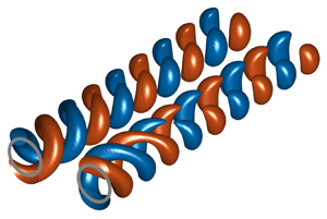
  $s/D=2.2$. As was done for figure 3, the streamwise amplification of the eigenfunctions is re-scaled with the growth rate of the most unstable one (SA1 in this case). As a result, the least amplified mode AA1 has its relative amplitude reduced along the streamwise direction. A phase mismatch also appears due to the small differences in $k_r$. The combination of the two modes is shown in figure 5(c,f): the pressure field behaves initially as two anti-symmetric counter-rotating helical modes, but soon evolves towards the sinuous lateral flapping of mode SA1.

Figure 5. Pressure eigenfunctions corresponding to twin jets with  $s/D = 2.2$ at $M_j=1.5, T_R = 1, R/\theta = 12.5$ and $St = 0.3$. The streamwise dependence is obtained from the corresponding eigenvalue, eliminating the spatial growth corresponding to SA1. (a–c) Iso-contours of the real pressure component. The grey circle shows the nozzle circumference. (d–f) Phase angle $\phi$ at a cylinder of radius 0.75 $D$ centred on one jet. Panels show (a) SA1; (b) AA1; (c) linear combination of SA1 and AA1.
3.3. Preferred mode of oscillation for finite-thickness twin jets
The results in the previous section suggest a strong dependence of the eigenvalue shift for all modes with frequency and jet separation. Figure 6 shows the results of a parametric study of the  $m=1$ modes for $St$ varying between 0.1 and 0.6 and $s/D$ varying between 1.8 and 5, extending the results of figure 4 for the twin jets with $M_j=1.5$, $T_R = 1$ and $R/\theta = 12.5$. Figure 6(a) shows the parametric regions in which each mode dominates, i.e. its spatial growth rate is the largest among the $m=1$ modes. Incidentally, it is noted that the growth rate of all $m=1$ is always larger than that of the $m=0$ modes, as expected for high $M_j$ jets with relatively thin shear layer (Michalke Reference Michalke1984). The alternating dependence of the leading mode with $s/D$ described before is also obtained with $St$, and the region of preference of the modes forms ‘stripes’ whose boundaries take approximately constant values of the product $St \times s/D$.

Figure 6. Preferred oscillation mode for twin jets as a function of the jet separation and Strouhal number. Here,  $M_j=1.5, T_R = 1, R/\theta = 12.5$. (a) Leading eigenmode. (b) Relative increase of the growth rate with respect to the single jet. (c) Same as (b), but colour coded to show the leading eigenmode. The same colour coding as figure 4 is used: blue: SS1; red: AS1; yellow: SA1; black: AA1.
Figure 6(a) provides no information on the relative growth rates of the leading mode with respect the others, or with respect to eigenmodes corresponding to a single jet. Figure 6(b) shows, for the leading eigenmode at each  $(St,s/D)$, the relative change in the growth rate resulting from the jet interaction, quantified as
 \begin{equation} \tilde{\Delta} k_i (St,s/D) = \dfrac{k_i(St,s/D) - k_i(St,s/D \to \infty)}{|k_i (St,s/D \to \infty)|}. \end{equation}
 Note that the dispersion relation for twin jets  $k(St,s/D)$ recovers that of a single jet in a smooth manner as $s/D \to \infty$. Each colour level in figure 6(b) corresponds to a relative increase of 1 % of $\tilde {\Delta } k_i$. The maximum colour level shown is 10 % but $\tilde {\Delta } k_i$ reaches larger values. As anticipated, the destabilisation of the leading eigenmode is inversely proportional to jet separation. For a fixed jet separation, the envelope of $|\tilde {\Delta } k_i|$ over all modes is also inversely proportional to $St$, similarly to the dependence on $s/D$ shown in figure 6(d). Consequently, as the product $St \times s/D$ increases, $\tilde {\Delta } k_i$ approaches zero. This happens in this case for regions dominated by the modes SS1 and AS1. Figure 6(c) shows again $\tilde {\Delta } k_i$, but colour coded to highlight the preferred oscillation mode. For the jet conditions analysed herein ( $M_j=1.5, T_R = 1, R/\theta = 12.5$), these results predict the dominance of mode SA1 leading to lateral sinuous oscillations for most jet separations and Strouhal numbers. The white regions in figure 6(c) correspond to conditions in which the jet interactions are weak, and hence do not lead to a substantial eigenvalue shift; the oscillation modes converge towards their behaviour for single jets for which there is no preferred mode. In this case, the jet may follow either a helical or flapping dynamics, which may be selected by other characteristics of the turbulent flow.
3.4. Influence of the shear-layer thickness
The results in previous sections were obtained for  $R/\theta = 12.5$, which corresponds to a relatively thin shear-layer thickness representative of axial distances around $0.5D$ downstream of the nozzle lip. This section considers the impact of the shear-layer thickness on the preferred oscillation mode for twin jets.
For high-speed jets,  $\theta$ grows approximately linearly with the distance from the nozzle. Crighton & Gaster (Reference Crighton and Gaster1976) use the analytical profile (3.1), obtaining a reasonable fit to the single-jet experiments by Crow & Champagne (Reference Crow and Champagne1971) with the approximation
 \begin{equation} \theta/R = 0.06 (x/D) + 0.04. \end{equation}
The experiments by Okamoto et al. (Reference Okamoto, Yagita, Watanabe and Kawamura1985) and Moustafa (Reference Moustafa1994) and the simulations by Goparaju & Gaitonde (Reference Goparaju and Gaitonde2018), to cite just a few, show that the shear-layer growth is also approximately linear with the axial distance to the nozzle for high-speed twin jets.
Michalke (Reference Michalke1984) discusses the impact of the shear-layer thickness on the locally parallel linear stability for single round jets. In the limit of very thin shear layers ( $R/\theta \to \infty$), all the eigenmodes are unstable and their spatial growth rates grow monotonically with $St$. As the jets develop downstream and the shear layer becomes thicker, the dispersion relation also changes; high frequencies are gradually stabilised and the range of unstable $St$ is reduced. The growth rate reduction resulting from the increase of the shear-layer thickness is proportional to the azimuthal number $m$. In consequence, modes $m=0$ and $m=1$ exhibit the largest growth rates, and which one of them dominates depends on the particular combination of parameters $M_j, T_R, R/\theta$ and $St$. However, increasing the jet Mach number favours helical modes over the axisymmetric ones, and for supersonic jets the $m=1$ mode presents, in general, larger growth rates.
The changes in the dispersion relation due to the downstream increase of the shear-layer thickness can also impact on the preferred flapping mode for twin jets at any given conditions. The relative change in the growth rate  $\tilde {\Delta } k_i$ used in the previous section (3.4) is not adequate for monitoring the preferred mode for relatively thicker shear layers, because the growth rate for the single jet $k_i(St,s/D \to \infty )$, that appears in the denominator, is no longer monotonic with $St$ and eventually vanishes and changes sign. Instead, the absolute change in the growth rate is considered here
 \begin{equation} \Delta k_i (St,s/D) = k_i(St,s/D) - k_i(St,s/D \to \infty). \end{equation}
 Figure 7 shows  $\Delta k_i$ and the growth rate $(-k_i)$ of the leading flapping mode at each $(St,s/D)$ for four values of the thickness parameter, $R/\theta =$ 12.5, 7.5, 5 and 3, which are representative of the shear-layer evolution from the nozzle lip to the end of the potential core, respectively $x/D \approx 0.67$, 1.6, 2.7 and 4.9 (Crighton & Gaster Reference Crighton and Gaster1976). The colours represent $\Delta k_i$ for the leading mode, coded as in figure 6. Each colour level corresponds to an absolute decrease (i.e. destabilisation) of $\Delta k_i = -0.01$. The solid lines show the growth rate $k_i(St,s/D)$ for the most unstable eigenmode. The absolute and relative changes in growth rate are qualitatively very similar for the very thin shear layer $R/\theta = 12.5$ (cf. figures 6(c) and 7(a)), as the leading mode is unstable. The striped structure of the preferred mode region is maintained as $R/\theta$ decreases, with a slow deviation of the stripes towards lower $St$.
$St$.

Figure 7. Preferred oscillation mode for twin jets as a function of the jet separation and Strouhal number. Here,  $M_j=1.5, T_R = 1$. Panels show (a) $R/\theta = 12.5$; (b) $R/\theta = 7.5$; (c) $R/\theta = 5$; (d) $R/\theta = 3$. Colours shows the absolute change of the growth rate with respect to the single jet, colour coded to show the leading eigenmode. Each colour level corresponds to an absolute decrease (i.e. destabilisation) of $\Delta k_i = -0.1$. The same colour coding as figure 4 is used: blue: SS1; red: AS1; yellow: SA1; black: AA1. The black solid lines show the growth rate $k_i(St,s/D)$ for the most unstable eigenmode. The thick black line corresponds to $k_i = 0$.
Combined with  $\Delta k_i$, the $k_i$ contours illustrate the relevance of the eigenvalue shift in the preference of the twin-jet system to present a certain mode of flapping over the others. For jet separations below $s/D \approx 3$, the magnitude of $\Delta k_i$ is comparable to $k_i$ and alters the growth rate of the leading mode significantly with respect to the single jet counterpart. For the first ${\sim }2D$ from the nozzle ( $R/\theta > 7.5$), local stability results predict the dominance of the sinuous flapping mode SA1 when the interaction between jets is relevant, i.e. for low $s/D$ values, while for large jet separations all the modes recover the single-jet behaviour. As with the shear-layer thickens, the range of unstable $St$ and the most unstable $St$ drop continuously. For $R/\theta = 3$, corresponding to a cross-stream plane close to the end of the potential core, the largest growth rate occurs for the mode AA1, instead of SA1. However, at this location the peak growth rate is considerably weaker than in the first two diameters of evolution.
Locally parallel instability analyses like those presented in figure 7 constitute a departure point for the exploration of spatially evolving flows and serve as base to non-parallel approaches like the multiple-scale expansion (Crighton & Gaster Reference Crighton and Gaster1976) or parabolised stability equations (Gudmundsson & Colonius Reference Gudmundsson and Colonius2011; Cavalieri et al. Reference Cavalieri, Rodríguez, Jordan, Colonius and Gervais2013; Rodríguez et al. Reference Rodríguez, Sinha, Brès and Colonius2013; Sinha et al. Reference Sinha, Rodríguez, Brès and Colonius2014; Rodríguez et al. Reference Rodríguez, Cavalieri, Colonius and Jordan2015). The dominant oscillation mode predicted at a certain downstream location does not depend on the local dispersion relation alone, but also on the integrated growth of the modes along the streamwise direction. However, present results show that the growth rate for all the  $m=1$ modes is substantially larger in the first few diameters of evolution, coincident with the conditions in which a preferential mode emerges. This suggests that the local instability results for thin shear layers can be used as a first approximation to predict the preferred oscillation mode in twin-jet configurations.
The results presented so far consider finite-thickness jets and are obtained using the linear stability analysis formulation described in § 2.1. While those calculations are performed using a personal computer, the parametric study leading to figure 6 requires the numerical solution of over 10 000 individual matrix eigenvalue problems, which becomes impractical for more comprehensive studies including the effect of the jet Mach number and the temperature ratio. In the following section, such a study is performed using the (zero-thickness) twin-jet shear-layer model presented in § 2.2.
3.5. Dependence of the preferred mode of oscillation on Mach number and temperature ratio
This section presents a parametric study of the effect of the jet Mach number  $M_j$ and temperature ratio $T_R$ on the preferred oscillation mode, using the vortex-sheet model for twin round jets. The description of the eigenmode families, the eigenvalue shift and their qualitative dependence on jet separation and Strouhal number given for finite-thickness jets holds for the vortex-sheet model. For each $(M_j,T_R)$, the evolution of the four $m=1$ eigenmodes with jet separation and Strouhal number is monitored in a manner analogous to that described in the previous section. The reduced computational cost of the vortex-sheet model computations allows for a greater region of interest and a significant refinement of the discretisation of the $(St,s/D)$ space. The analysis for one $(M_j,T_R)$ case involves the calculation of nearly 1.5 million eigenvalues, but takes less than an hour on a modern personal computer.
Figure 8 shows the leading oscillation mode for twin jets with  $T_R = 1$ and $M_j$ between 1 and 2. The overall picture reproduces that already described for the finite-thickness $M_j = 1.5$ case:
(i) the regions in which each particular mode dominates in the
$(St,s/D)$ space form alternating stripes;(ii) the maximum eigenvalue shift, computed following (3.4), occurs for the smallest jet separation within each strip;
(iii) as the jet separation is reduced, the Strouhal number for the maximum shift of the growth rate is increased.


Figure 8. Preferred oscillation mode for twin jets as a function of the jet separation and Strouhal number. Vortex-sheet model,  $T_R = 1$ and varying $M_j$. Contours as in figure 6(c). Blue: SS1; red: AS1; yellow: SA1; black: AA1.
For  $M_j = 1$ (figure 8a) and $s/D \le 3$, mode SS1 dominates for $St \le 0.2$. For larger $St$, modes SA1 and AA1 become dominant but their eigenvalue shift is comparatively weak. Increasing the jet Mach number at constant temperature ratio has two effects. First, the boundaries of the mode stripes are gradually displaced towards lower $St$ and $s/D$ values. Second, the shift of the growth rates is increased. The latter implies that the interaction between the fluctuation fields of the two jets intensifies with $M_j$. The combination of the two effects leads to the gradual appearance of a new stripe of mode SS1 at higher $St$ while the corresponding stripe at the lower $St$ region reduces. Simultaneously, the stripe of mode SA1 is displaced to lower Strouhal numbers while its growth rate shift is increased. For $M_j$ above 1.5, mode SA1 (sinuous lateral oscillations) has the largest growth rate shift.
For  $M_j$ above 1.6 (figure 8d–f), the results for mode SA1 present an anomalous behaviour in the limit of lower separation and Strouhal number, that is clearly visible in the figures. Instead of following the general trend, the boundary of the stripe forms a horizontal segment (constant $St$) for $s/D$ below a threshold value increases with $M_j$. A preliminary study revealed that this anomaly is due to the appearance of a saddle point in the evolution of mode SA1, which pinches with mode SA2 at a certain $(St,s/D)$ combination. This saddle point is not associated with an absolute instability, as it involves two downstream-propagating K–H eigenmodes. A deep study regarding this issue is currently underway but is beyond the scope of this paper.
Figure 9 shows the parametric study for twin jets with fixed jet Mach number  $M_j = 1.5$ and temperature ratio increasing from $T_R = 1$ to 4. The effect of increasing the jet temperature follows the same trends as increasing the jet Mach number: the mode stripes move towards lower $St$ and $s/D$, reducing the region dominated by mode SS1 (dominant for $T_R = 1$) and increasing the relative importance of mode SA1 with increasing temperature. Overall, the impact of the temperature ratio on the eigenmode shift is weaker than that of the jet Mach number, but still mode SA1 attains growth rates nearly 10 % larger than those for the equivalent single jet.

Figure 9. Preferred oscillation mode for twin jets as a function of the jet separation and Strouhal number. Vortex-sheet model,  $M_j = 1.5$ and varying $T_R$. Contours as in figure 6(c). Blue: SS1; red: AS1; yellow: SA1; black: AA1.
4. Conclusions
Linear stability theory is often used to model the large-scale flow structures in the turbulent mixing region and near pressure field of high-speed jets. For perfectly expanded single round jets, these models predict the dominance of  $m=1$ helical modes for relatively low frequencies and thin shear layers, in agreement with empirical data.
For twin-jet configurations, the interaction between their fluctuation fields results in coupling. The symmetries present in the geometry lead to a separation of the modes into four families, corresponding to the even/odd behaviour of the pressure field about the symmetry plane and the plane containing the jet axes. The division into families is inherent to the twin-jet geometry and not just an artefact of the problem formulation: while it is exploited here to simplify the analyses, a formulation in which the symmetries/anti-symmetries are not imposed recovers the same families (Rodríguez et al. Reference Rodríguez, Jotkar and Gennaro2018). The fluctuation field associated with  $m = 1$ modes for twin jets does not correspond to helical oscillations, but to flapping oscillations of the jet.
The coupling between the jets is quantified by monitoring the shift of the complex wavenumber  $k$ (eigenvalue of the spatial linear stability problem) with respect to that of the single jet, $\Delta k$. The absolute value of $\Delta k$ is different for each oscillation mode, but for all of them is inversely proportional to both the jet separation $s/D$ and the Strouhal number $St$. However, the real and imaginary parts of $\Delta k$ do not present a monotonic dependence on $St$ or $s/D$. This leads to regions in the $(St,s/D)$ space in which different modes of oscillation dominate over others.
The thickness of the jet's shear layer, that has a strong impact on the spatial growth rate for all eigenmodes and Strouhal numbers, is found to have a mild effect on the preferred  $m=1$ mode for a given $(St,s/D)$ condition. Incidentally, the growth rate for these eigenmodes is much larger during the first few diameters from the nozzle, where the shear layer is thinner; if the amplification of a particular flapping mode dominates during the initial 1–2 diameters, it is likely to remain the preferred one at downstream locations. This suggests that the local instability results in the limit of thin shear layers can be used to predict the preferred oscillation mode, at least, to extent of the potential core. However, it is to be noted that other factors, such as nonlinear interactions between modes leading to their early saturation or a rigorous downstream integration of the modes amplitudes, aspects that are not considered in the present work, can offer improved predictions.
A parametric study for zero-thickness shear-layer jets is presented in which the jet Mach number  $M_j$ is varied between 1 and 2, and the jet temperature ratio $T_R$ is varied between 1 and 4. Increasing independently both $M_j$ and $T_R$ is found to augment the jet coupling and modify the $(St,s/D)$ map of the preferred oscillation mode. Present results predict that only two oscillation modes are likely to be observed when jet coupling is relevant, namely in-phase (varicose) or counter-phase (sinuous) flapping oscillations on the plane containing the nozzles (modes SS1 and SA1, respectively).
It should be noted that while flapping modes are the natural mode of oscillation of twin jets, a superposition of them may still generate some helical motions in regions close to the nozzle. However, owing to the differences between the growth rates of each mode and their exponential amplification in the first few diameters, it can be expected that flapping motions will dominate the flow as it develops downstream. Hence, the eventual helical oscillations in twin-jet systems would be a spatially transient feature of the flow.
The results presented in this work consider perfectly expanded jets. The preference of certain oscillation modes over others is predicted based on the larger growth rate of the corresponding K–H instability eigenmode. It may be expected that these results would be applicable also to shock-containing jets, at least to some extent. The preference of shock-containing twin jets to present flapping motions at conditions in which a single jet presents helical motions has been shown by different authors (Seiner et al. Reference Seiner, Manning and Ponton1988; Wlezien Reference Wlezien1989; Kuo et al. Reference Kuo, Cluts and Samimy2017; Knast et al. Reference Knast, Bell, Wong, Leb, Soria, Honnery and Edgington-Mitchell2018; Bell et al. Reference Bell, Soria, Honnery and Edgington-Mitchell2018, Reference Bell, Cluts, Samimy, Soria and Edgington-Mitchell2021). However, one should be cautious when extending the present conclusions to shock-containing jets. As these jets are subjected to the resonance loop associated with screech (Powell Reference Powell1953; Edgington-Mitchell Reference Edgington-Mitchell2019; Nogueira et al. Reference Nogueira, Jordan, Jaunet, Cavalieri, Towne and Edgington-Mitchell2022b), the actual dominant oscillation is a function of the symmetry associated with the most globally unstable resonance mode. As shown in Tam & Tanna (Reference Tam and Tanna1982), Edgington-Mitchell et al. (Reference Edgington-Mitchell, Wang, Nogueira, Schmidt, Jaunet, Duke, Jordan and Towne2021), Nogueira & Edgington-Mitchell (Reference Nogueira and Edgington-Mitchell2021), Nogueira et al. (Reference Nogueira, Jaunet, Mancinelli, Jordan and Edgington-Mitchell2022a) and Edgington-Mitchell et al. (Reference Edgington-Mitchell, Li, Liu, He, Wong, Mackenzie and Nogueira2022), the closure mechanism of screech is strongly dependent on the wavenumber of the waves involved in resonance, and less dependent on the growth rate of the K–H instability. However, as the wavenumber of the K–H eigenmode is one of the driving components of this phenomenon, the present results remain relevant: they may be used as input for screech models in twin jets and help explain the preferred flapping mode in shock-containing jets as well.
Funding
D.R. is funded by the Government of the Community of Madrid within the multi-annual agreement with Universidad Politécnica de Madrid through the Program of Excellence in Faculty (V-PRICIT line 3) and the Program of Impulse of Young Researchers (V-PRICIT lines 1 and 3, Grant No. APOYO-JOVENES-WYOWRI-135-DZBLJU). M.N.S. is supported through an Australian Government Research Training Program Scholarship. P.A.S.N. and D.M.E.M. were supported by the Australian Research Council through the Discovery Project scheme (Grant No. DP190102220).
Declaration of interests
The authors report no conflict of interest.


 Open access