


1. Introduction
This study investigates water waves generated by an obstacle moving along the sea bottom. Many analytical studies on this subject exist. In the simplest scenario, Tinti, Bortolucci & Chiavettieri (Reference Tinti, Bortolucci and Chiavettieri2001) solved the linear shallow water wave equations in 1DH (one-dimensional in the horizontal direction) constant depth for waves generated by a bottom obstacle that suddenly begins travelling at a constant speed. Closed-form solutions, reflecting the existence of three different waves, were obtained. Didenkulova, Nikolkina & Pelinovsky (Reference Didenkulova, Nikolkina and Pelinovsky2011) and Lo & Liu (Reference Lo and Liu2017) examined the resonance case more closely. By cross-sectional averaging, Didenkulova & Pelinovsky (Reference Didenkulova and Pelinovsky2013) extended the analysis to narrow bays and channels. For linear long waves generated by a deformable bottom boundary on a slope in 1DH, Tuck & Hwang (Reference Tuck and Hwang1972) derived the general integral-form analytical solutions consisting of three integrals. These integrals need to be numerically integrated. Liu, Lynett & Synolakis (Reference Liu, Lynett and Synolakis2003) found a special case for which the integral-form solution can be simplified to only one integral. Another special case for which a closed-form solution exists was found by Lo & Liu (Reference Lo and Liu2017). Simplified solutions were also found by Didenkulova et al. (Reference Didenkulova, Nikolkina, Pelinovsky and Zahibo2010) on a convex slope.
In 2DH (two-dimensional in the horizontal direction), Sammarco & Renzi (Reference Sammarco and Renzi2008) first derived analytical solutions for bottom-obstacle-generated linear long waves on a plane beach. Renzi & Sammarco (Reference Renzi and Sammarco2010) extended the analysis to consider the wave propagation around a conical island. While these 2DH analytical solutions are exact and the 2DH configuration is more realistic than a 1DH one, the analytical solutions are in a complex form comprising an infinite series and multiple integrals that need to be evaluated numerically. Therefore, they cannot be easily analysed or used. Solving the linear shallow water equations directly using numerical methods may be more convenient in practice, as discussed by Lo & Liu (Reference Lo and Liu2017). To date, closed-form analytical expressions linking the obstacle parameters to the water wave characteristics in 2DH are still lacking.
The main intended application of these studies are tsunamis generated by a landslide. Some historical landmark events include: the 1958 Lituya Bay megatsunami, where a subaerial landslide generated water waves producing a local runup height of up to  $524$ m (see e.g. Fritz, Mohammed & Yoo Reference Fritz, Mohammed and Yoo2009); the 1998 Papua New Guinea tsunami, which resulted in over
  $2000$ casualties and affected at least
  $25$ km of coastline, is commonly believed to have been caused by a submarine landslide (see e.g. Lynett et al. Reference Lynett, Borrero, Liu and Synolakis2003); most recently, the 2018 Sulawesi earthquake and tsunami, which resulted in over
  $4000$ casualties, is believed to have been caused by a combination of tectonic and landslide sources (see e.g. Liu et al. Reference Liu, Higuera, Husrin, Prasetya, Prihantono, Diastomo, Pryambodo and Susmoro2020). While subaerial landslides, or submarine landslides occurring very close to shore, are capable of generating waves of extremely large amplitudes (such as the 1958 Lituya Bay tsunami), their area of impact is generally confined and local. On the other hand, submarine landslides occurring in the open ocean, most likely on continental slopes, are larger (longer) in scale and thus have the potential for generating regional tsunamis, such as the 1998 Papua New Guinea tsunami.
To more realistically model landslide-generated tsunamis, more complex theoretical formulations have been proposed. On a slope in 1DH, Özeren & Postacioglu (Reference Özeren and Postacioglu2012) obtained analytical solutions to the nonlinear shallow water wave equations for landslide-generated tsunamis using hodograph transforms. Wang, Liu & Mei (Reference Wang, Liu and Mei2011) adopted the lubrication theory to allow for a self-evolving solid landslide, coupled with the nonlinear shallow water wave equations. In 2DH, Couston, Mei & Alam (Reference Couston, Mei and Alam2015) considered nonlinear long waves in the Lagrangian frame of reference to investigate landslide tsunamis in lakes. While more complex and realistic, these formulations all need to be resolved by numerical methods. Of course, in practical applications, numerical models are the most prevalent tools for studying landslide-generated tsunamis (see e.g. Løvholt et al. Reference Løvholt, Pedersen, Harbitz, Glimsdal and Kim2015 for a review); alternatively, reciprocal Green's functions can also be employed for fast forecasting (see e.g. Chen et al. Reference Chen, Liu, Wijetunge and Wang2020).
As pointed out in the review paper by Løvholt et al. (Reference Løvholt, Pedersen, Harbitz, Glimsdal and Kim2015), a clear knowledge gap exists in the link between the parameters of a landslide and its tsunamigenic potential. We see this missing piece of knowledge as an analogy to Okada's model, which is widely used to study earthquake-generated tsunamis. Using the linear elastic dislocation model, Okada (Reference Okada1985) derived analytical expressions linking the fault plane parameters of an earthquake to the resulting seafloor displacement. The earth was assumed to be flat and a homogeneous isotropic elastic material, and the fault plane was assumed to be a rectangular patch. To model the tsunami generated by the seafloor displacement, the seafloor displacement is often assumed to be instantaneous, and the corresponding water surface displacement mimics the seafloor displacement. The free surface displacement is then used as the initial condition for a tsunami propagation model of choice, in which complex bathymetry data can be considered. Despite the numerous idealisations in this sequence of approximations, this approach has served as the standard in conventional modelling of earthquake-generated tsunamis. The main justification for these simplifications is that great uncertainties inherently exist in the earthquake and fault parameters, and thus more accurately modelling the resulting seafloor and water surface displacements brings only minimal benefits. For a review on tsunami modelling, readers are referred to Saito (Reference Saito2017) and Grezio et al. (Reference Grezio2017).
In the landslide–tsunami research community, however, such an analytical model linking the landslide parameters to the water waves is lacking. While many scholars had investigated this issue for submarine landslides (see e.g. Striem & Miloh Reference Striem and Miloh1976; Pelinovsky & Poplavsky Reference Pelinovsky and Poplavsky1996; Watts Reference Watts1998; Murty Reference Murty2003), none of them provided a universal model that can be widely applied in practical applications. To date, the most commonly used model for prescribing the tsunami generated by a submarine landslide is that proposed by Grilli & Watts (Reference Grilli and Watts2005) and Watts et al. (Reference Watts, Grilli, Tappin and Fryer2005). However, their model is purely empirical, relying on parameter tuning to acquire best-fitting results. Therefore, it cannot be used in predictive studies. On the other hand, although subaerial landslides are beyond the scope of this study, we acknowledge that significant research efforts have been poured into deriving empirical equations to describe water waves generated by subaerial landslides (see e.g. Fritz, Hager & Minor Reference Fritz, Hager and Minor2003; Heller & Hager Reference Heller and Hager2010; Heller & Spinneken Reference Heller and Spinneken2015). Without a simple landslide–wave generation model linking the landslide parameters to the water waves, the entire landslide–wave generation process must be simulated, which is computationally costly and severely hinders probabilistic hazard assessment studies.
The present study attempts to fill this knowledge gap in the wave generation process by submarine landslides. By deriving new analytical solutions and extracting new insights from the results, we seek to pave the way for the construction of a simple theory-based wave generation model for landslide tsunamis, analogous to Okada's model for earthquake tsunamis. The simplest configuration consisting of a solid obstacle translating along the bottom boundary in 2DH constant water depth at a prescribed speed is considered. Only subcritical forcing speeds are discussed in this study. Linear analytical investigations are first presented in § 2. Closed-form asymptotic solutions, clearly reflecting the scaling relations between the obstacle and the water waves it generates, are derived. To address the shortcomings of the linear analytical solutions, numerical investigations are conducted in § 3. More specifically, the deviations from the analytical solutions due to nonlinear effects, obstacle acceleration effects and obstacle deceleration effects are investigated numerically. In § 4, we conclude the study and share recommendations for future studies.
2. Analytical solutions
This study examines inviscid, incompressible and irrotational water waves generated by a moving bottom obstacle in constant water depth in the three-dimensional space. Hence, the free surface waves are two-dimensional in the horizontal space (2DH). The moving bottom obstacle is interpreted as a deformable bottom boundary. As sketched in figure 1 using dimensional quantities, the bottom boundary deformation caused by the moving obstacle is captured by  $B'(x',y',t')$. The obstacle is a solid with a characteristic length of
  $L$ and a maximum thickness of
  $A$. The constant water depth is
  $d$. The free surface elevation
  $\eta '(x',y',t')$ is defined as the displacement of the free surface from the still water level, which is located at
  $z'=0$. Here,
  $L$ is chosen as the characteristic horizontal length scale,
  $A$ is chosen as the characteristic vertical length scale, the linear long-wave celerity
  $\sqrt {gd}$, in which
  $g$ denotes the gravitational acceleration, is chosen as the characteristic speed and hence the characteristic time scale is
  $L/\sqrt {gd}$. The variables are then normalised as follows:
 \begin{equation} (x,y,z,t)=\left(\frac{x'}{L},\frac{y'}{L},\frac{z'}{d},\frac{t'}{L/\sqrt{gd}}\right), \quad (B,\eta)=\left(\frac{B'}{A},\frac{\eta'}{A}\right). \end{equation}
Figure 1. A dimensional definition sketch of water waves generated by a moving bottom obstacle. Both the free surface displacement and the thickness of the obstacle are assumed small in linear wave models; such assumptions are not needed in nonlinear wave models. This study considers only bottom obstacles translating at a subcritical speed.
The linear and fully dispersive wave model (hereinafter LFD) for such a flow problem is well known (see e.g. Mei, Stiassnie & Yue Reference Mei, Stiassnie and Yue2005). The Laplace equation, which is the continuity equation for incompressible and irrotational flows, and the linearised boundary conditions are
 \begin{equation} \left.\begin{array}{rr@{}} \mu^2\phi_{xx}+\mu^2\phi_{yy}+\phi_{zz}=0, & -1< z<0, \\ \phi_z=\mu^2 B_t, & z={-}1, \\ \phi_z=\mu^2 \eta_t, & z=0, \\ \phi_t+\eta=0, & z=0, \end{array} \right\} \end{equation}
where  $\phi (x,y,z,t)=\phi '(x',y',z',t')/(\epsilon L\sqrt {gd})$ is the velocity potential. The parameter
  $\epsilon =A/d$ measures how strong nonlinearity is. In a linear wave model,
  $\epsilon$ is assumed to be small – both the water surface displacement and the bottom boundary deformation are assumed small in comparison with the water depth. On the other hand, the parameter
  $\mu =d/L$ is a measure of how strong frequency dispersion is. In (2.2), no assumptions are made regarding the order of magnitude of
  $\mu$. Hence, this wave system is fully dispersive.
The system of equations in (2.2) is a classical linear wave problem and can be solved by applying the Laplace and Fourier transforms. In this study, the Fourier transform of a function  $f(x)$ is defined as
 \begin{equation} \bar{f}(k)=\frac{1}{\sqrt{2{\rm \pi}}}\int_{-\infty}^\infty f(x) \ \textrm{e}^{-\textrm{i}kx}\,{\textrm{d}\kern0.7pt x}, \quad f(x)=\frac{1}{\sqrt{2{\rm \pi}}}\int_{-\infty}^\infty\bar{f}(k) \ \textrm{e}^{\textrm{i}kx}\,\textrm{d}k , \end{equation}
where the bar denotes Fourier transformation in the  $x$ direction. A wide tilde will be used to denote that in the
  $y$ direction. Whereas
  $k$ is the wavenumber in the
  $x$-space,
  $l$ is the wavenumber in the
  $y$-space. On the other hand, in this study, the Laplace transform of a function
  $f(t)$ is defined as
 \begin{equation} \dddot{f}(s)=\int_{0}^\infty f(t) \ \textrm{e}^{{-}st}\,\textrm{d}t, \quad f(t)=\frac{1}{2{\rm \pi} i}\lim_{T\to\infty}\int_{\gamma-\textrm{i}T}^{\gamma+\textrm{i}T}\dddot{f}(s) \ \textrm{e}^{st}\,\textrm{d}s , \end{equation}
where the triple dots denote a Laplace transformed function, and  $\gamma$ is a vertical contour in the complex plane chosen so that all singularities of
  $\dddot {f}(s)$ are to the left of it.
After Fourier–Laplace transforming (2.2) and simplifying, the transformed solution reads
 \begin{align} \dddot{\tilde{\bar{\phi}}}&=\frac{1}{\cosh\mu q}\frac{1}{s^2+q^2D^2} \left(\left(s\widetilde{\overline{\phi(x,y,0,0)}}-\widetilde{\overline{\eta(x,y,0)}}\right)\cosh\left(\mu q(z+1)\right) \right.\nonumber\\ &\quad\left. -\left(s\dddot{\tilde{\bar{B}}}-\widetilde{\overline{B(x,y,0)}}\right)\cosh(\mu q z) +\frac{\mu s^2}{q}\left(s\dddot{\tilde{\bar{B}}}-\widetilde{\overline{B(x,y,0)}}\right)\sinh(\mu q z) \right), \end{align}
where
 \begin{equation} q=\sqrt{k^2+l^2} \end{equation}
will be used throughout the study to simplify the expressions, and
 \begin{equation} D=\sqrt{\frac{\tanh(\mu q)}{\mu q}} \end{equation}
is the normalised wave celerity of linear dispersive waves in 2DH constant depth. Here,  $D(\mu q)$ is plotted in figure 2 as a function of
  $\mu q$ – it has a maximum of one at
  $\mu q=0$, and decays to zero as
  $\mu q$ increases. We note that
  $q\geqslant 0$ according to (2.6).

Figure 2. The LFD wave celerity  $D$ in (2.7), plotted as a function of
  $\mu q$.
The transformed free surface  $\dddot {\tilde {\bar {\eta }}}$ can be recovered as
 \begin{equation} \dddot{\tilde{\bar{\eta}}}={-}s\dddot{\widetilde{\overline{\phi(x,y,0,t)}}}+\widetilde{\overline{\phi(x,y,0,0)}}{\,\,.} \end{equation}
The velocity components in the  $x$,
$x$,  $y$ and
  $z$ directions –
  $u(x,y,z,t)$,
  $v(x,y,z,t)$ and
  $w(x,y,z,t)$, respectively – can be calculated from the velocity potential as
 \begin{equation} u=\phi_x, \quad v=\phi_y, \quad w=\phi_z. \end{equation}
2.1. Complete integral-form solutions
In order to acquire more specific solutions, further assumptions need to be made. Firstly, the initial conditions to impose in solving (2.2) are specified as
 \begin{equation} \eta(x,y,0)=0, \quad \phi(x,y,0,0)=\textrm{const}. \end{equation}
Whereas  $\eta (x,y,0)=0$ means an initially flat water surface,
  $\phi (x,y,0,0)=\textrm {const.}$ means zero initial horizontal velocities on the still water surface,
  $z=0$.
Second, we consider a bottom obstacle that suddenly starts moving in the  $x$ direction at a constant speed of
  ${\mathit {Fr}}>0$ for
  $t>0$, where the Froude number
  ${\mathit {Fr}}$ is defined as the dimensional obstacle speed
  $U_B$ divided by the linear long-wave celerity
 \begin{equation} {\mathit{Fr}}=\frac{U_B}{\sqrt{gd}}. \end{equation}
Such an idealisation is necessary for obtaining closed-form analytical solutions. This sudden motion essentially corresponds to an infinitely large initial acceleration of the obstacle. More discussions on the effects of acceleration will be provided in § 3.3. For consistency and without loss of generality, the coordinate system shall be defined such that the centre of mass of the bottom obstacle  $B$ is located at the origin
  $(x,y)=(0,0)$ at
  $t=0$.
We emphasise that, although no assumptions on the magnitude of  ${\mathit {Fr}}$ are needed to derive the complete integral-form solutions, this study considers only bottom obstacles translating at a subcritical speed, i.e.
  $0<{\mathit {Fr}}<1$. The two main reasons are: first, the wave characteristics due to subcritical, critical and supercritical
  ${\mathit {Fr}}$ are fundamentally different, and this study seeks to maintain a clear focus on the subcritical case. Second, the primary intended application of this study is to provide basic scaling estimates for tsunamis generated by a submarine landslide. A submarine landslide is unlikely to travel faster than a subcritical speed. For example, in a water depth of
  $1500$ m, which is the source depth estimate by Watts et al. (Reference Watts, Grilli, Kirby, Fryer and Tappin2003) for the 1998 Papua New Guinea landslide tsunami, the corresponding critical speed is
  $121\ \textrm {m}\ \textrm {s}^{-1}$, or
  $436\ \textrm {km}\ \textrm {h}^{-1}$. On the other hand, a subaerial landslide, or a submarine landslide occurring very close to shore, is more likely to travel at a supercritical speed due to the initially extremely shallow water depth. Nonetheless, subaerial landslides are beyond the scope of this study.
For a bottom obstacle translating at speed  ${\mathit {Fr}}$, the bottom obstacle function can be written as
 \begin{equation} B(x,y,t)=B(x-{\mathit{Fr}} t,y) \end{equation}
and its Fourier transform is
 \begin{equation} \tilde{\bar{B}}(k,l,t)=\widetilde{\overline{B(x,y,0)}}\exp({-\textrm{i}k {\mathit{Fr}} t})=\widetilde{\overline{B_0(x,y)}}\exp({-\textrm{i}k {\mathit{Fr}} t}). \end{equation}
For convenience, we define  $B_0(x,y)=B(x,y,0)$ as the bottom obstacle shape function that excludes the translation. Laplace transforming (2.13) gives
 \begin{equation} \dddot{\tilde{\bar{B}}}=\widetilde{\overline{B_0}}(k,l)\frac{1}{s+\textrm{i} k {\mathit{Fr}}}. \end{equation}
After specifying the bottom obstacle function as (2.14) and imposing the initial conditions (2.10a,b), the expression for the transformed free surface (2.8) becomes
 \begin{equation} \dddot{\tilde{\bar{\eta}}}(k,l,s)=\frac{-\textrm{i} k {\mathit{Fr}} \widetilde{\overline{B_0}}}{\cosh(\mu q)}\frac{s}{s+\textrm{i}k {\mathit{Fr}}}\frac{1}{s^2+q^2 D^2}, \end{equation}
for which the closed-form inverse Laplace transform is available:
 \begin{align} \tilde{\bar{\eta}}(k,l,t)&=\frac{\widetilde{\overline{B_0}}}{\cosh(\mu q)} \left(-\frac{{\mathit{Fr}}^2\dfrac{k^2}{q^2}}{D^2-{\mathit{Fr}}^2\dfrac{k^2}{q^2}}\exp({-\textrm{i}k {\mathit{Fr}} t})+\dfrac{{\mathit{Fr}}\dfrac{k}{q}}{2\left(D-{\mathit{Fr}}\dfrac{k}{q}\right)}\exp({-\textrm{i}q\,\textrm{D}t})\right.\nonumber\\ &\quad \left. - \dfrac{{\mathit{Fr}}\dfrac{k}{q}}{2\left(D+{\mathit{Fr}}\dfrac{k}{q}\right)}\exp({\textrm{i}q\,\textrm{D}t})\right). \end{align}
Noting the different wave components and writing out the definition of the inverse Fourier transform, we then have the complete analytical solution in integral form as
 \begin{equation} \left. \begin{array}{l@{}} \displaystyle \eta(x,y,t)=\eta_{{{\mathit{Fr}}}}(x,y,t)+\eta_{+}(x,y,t), \\ \displaystyle \eta_{{{\mathit{Fr}}}}(x,y,t) ={-}\dfrac{1}{2{\rm \pi}}\int_{-\infty}^{\infty}\int_{-\infty}^{\infty} \dfrac{\widetilde{\overline{B_0}}(k,l)}{\cosh(\mu q)}\dfrac{{\mathit{Fr}}^2\dfrac{k^2}{q^2}}{D^2-{\mathit{Fr}}^2\dfrac{k^2}{q^2}}\\ \qquad\qquad\quad\times\exp({-\textrm{i}k {\mathit{Fr}} t}) \exp({\textrm{i}kx})\exp({\textrm{i}ly})\,\textrm{d}k\,\textrm{d}l, \\ \displaystyle \eta_{+}(x,y,t)=\dfrac{1}{2{\rm \pi}}\int_{-\infty}^{\infty}\int_{-\infty}^{\infty} \dfrac{\widetilde{\overline{B_0}}(k,l)}{\cosh(\mu q)}\\ \qquad\qquad\quad\times\left(\dfrac{{\mathit{Fr}}\dfrac{k}{q}}{2\left(D-{\mathit{Fr}}\dfrac{k}{q}\right)} \exp({-\textrm{i}q\,\textrm{D}t})-\dfrac{{\mathit{Fr}}\dfrac{k}{q}}{2\left(D+{\mathit{Fr}}\dfrac{k}{q}\right)} \exp({\textrm{i}q\,\textrm{D}t})\right)\\ \qquad\qquad\quad \times\exp({\textrm{i}kx})\exp({\textrm{i}ly})\,\textrm{d}k \,\textrm{d}l. \end{array} \right\} \end{equation}
With a moving coordinate that follows the bottom obstacle,  $\xi =x-{\mathit {Fr}} t$,
  $\eta _{{\mathit {Fr}}}(x,y,t)$ can be expressed as
  $\eta _{{\mathit {Fr}}}(\xi ,y)$. Thus,
  $\eta _{{\mathit {Fr}}}$ is a steady-state solution in the moving coordinate. It is a ‘trapped wave’ of permanent shape that moves with the bottom obstacle. More discussions on the trapped wave solution will be provided in § 2.5. On the other hand,
  $\eta _{+}$ represents transient free waves that travel at a speed of
  $D$ (as indicated by the
  $\exp({\rm i}q\, {\rm D}t)$ and
  $\exp(-{\rm i}q\, {\rm D}t)$ terms), which is the linear dispersive wave speed for the wave component
  $\mu q$.
In 2DH, it is often more convenient to express the solutions in polar coordinates. By using the substitutions  $x=r\cos \theta$,
  $y=r\sin \theta$,
  $k=q\cos \psi$ and
  $l=q\sin \psi$, the integral-form solutions (2.17) can be written as
 \begin{equation} \left. \begin{array}{l@{}} \displaystyle \eta(r,\theta,t)=\eta_{{{\mathit{Fr}}}}(r,\theta,t)+\eta_{+}(r,\theta,t), \\ \displaystyle \eta_{{{\mathit{Fr}}}}(r,\theta,t)={-}\dfrac{1}{2{\rm \pi}}\int_{0}^{2{\rm \pi}}\int_{0}^{\infty} \dfrac{q\widetilde{\overline{B_0}}(q,\psi)}{\cosh(\mu q)}\dfrac{{\mathit{Fr}}^2\cos^2\psi}{D^2-{\mathit{Fr}}^2\cos^2\psi}\\ \qquad\qquad\quad\displaystyle\times\exp({-\textrm{i}q {\mathit{Fr}}(\cos\psi) t}) \exp({\textrm{i}qr\cos(\psi-\theta)})\,\textrm{d}q\,\textrm{d}\psi, \\ \displaystyle \eta_{+}(r,\theta,t)=\dfrac{1}{2{\rm \pi}}\int_0^{2{\rm \pi}}\int_0^\infty \dfrac{q\widetilde{\overline{B_0}}(q,\psi)}{\cosh(\mu q)}\\ \qquad\qquad\quad\displaystyle\times \left( \dfrac{{\mathit{Fr}}\cos\psi}{2(D-{\mathit{Fr}}\cos\psi)}\exp({-\textrm{i}q\,\textrm{D}t})- \dfrac{{\mathit{Fr}}\cos\psi}{2(D+{\mathit{Fr}}\cos\psi)}\exp({\textrm{i}q\,\textrm{D}t})\right)\\ \qquad\qquad\quad\displaystyle \times\exp({\textrm{i}qr\cos(\psi-\theta)})\,\textrm{d}q\,\textrm{d}\psi . \end{array} \right\} \end{equation}
In a similar manner, the integral-form solutions for the velocities can be obtained from (2.5) and (2.9a–c). The exact expressions are provided in the supplementary material available at https://doi.org/10.1017/jfm.2021.537.
Discontinuities exist in the solutions for  $D(q)=\pm {\mathit {Fr}}\cos \psi$. In Appendix A, we show that these discontinuities either are integrable based on the Cauchy principal value, or end up cancelled out by each other. Thus, when numerically integrating the complete integral-form solutions, small regions near the discontinuities can be omitted, since their net contribution to the integration is zero.
Lastly, we verify that if a 1DH bottom obstacle function is used, i.e.  $B(x,y,t)=B(x,t)$, its Fourier transform becomes
  $\tilde {\bar {B}}(k,l,t)=\bar {B}(k,t) \delta (l) \sqrt {2{\rm \pi} }$, where
  $\delta (l)$ is the Dirac delta function, and the 1DH solutions as derived in Lo & Liu (Reference Lo and Liu2017) can be recovered.
2.2. Far-field asymptotic solutions,  $r\to \infty$

To reduce the complexity of the integral-form solutions and increase their usability, asymptotic solutions can be sought. For the subcritical speed  $0<{\mathit {Fr}}<1$, the free wave
  $\eta _+$ is able to travel faster than the trapped wave
  $\eta _{\mathit {Fr}}$, and eventually the free wave separates from the trapped wave to become the leading wave. Hence, it is sufficient to consider only
  $\eta _+$ in the far field where
  $r$ is large. For large
  $r$, the stationary phase approximation can be applied to the
  $\psi$-integral in the expression for
  $\eta _+$ given in (2.18). The phase function
  $q\cos (\psi -\theta )$ has stationary points at
  $\psi _0=n{\rm \pi} +\theta$, where
  $n$ is an integer. For easier application of the stationary phase approximation, we shift the integration limits for
  $\psi$ to the left by a small distance so that
  $\psi _0=\theta , {\rm \pi}+\theta$ are the two stationary points contained in the interval (this is permissible as the integrand is periodic in
  $\psi$ with a period of
  $2{\rm \pi}$). The main contributions to the integral then come from the vicinity of
  $\psi =\theta$ and
  $\psi ={\rm \pi} +\theta$, and the
  $\psi$-integrals can be approximated for large
  $r$ as
 \begin{align} \eta_{+}&\simeq{-}\frac{1}{\sqrt{2{\rm \pi}}}r^{-{1}/{2}}\int_0^\infty\frac{\widetilde{\overline{B_0}}(q,{\rm \pi}+\theta)}{\cosh(\mu q)}\frac{{\mathit{Fr}}\cos\theta}{2(D+{\mathit{Fr}}\cos\theta)}q^{1/2} \exp\left({-\textrm{i}\left(q(r+\textrm{D}t)-\frac{\rm \pi}{4}\right)}\right)\textrm{d}q\nonumber\\ &\quad+\frac{1}{\sqrt{2{\rm \pi}}}r^{-{1/2}}\int_0^\infty\frac{\widetilde{\overline{B_0}}(q,\theta)}{\cosh(\mu q)}\frac{{\mathit{Fr}}\cos\theta}{2(D-{\mathit{Fr}}\cos\theta)}q^{1/2} \exp\left({\textrm{i}\left(q(r-\textrm{D}t)-\frac{\rm \pi}{4}\right)}\right)\textrm{d}q \nonumber\\ &\quad+\frac{1}{\sqrt{2{\rm \pi}}}r^{-{1/2}}\int_0^\infty\frac{\widetilde{\overline{B_0}}(q,{\rm \pi}+\theta)}{\cosh(\mu q)}\frac{{\mathit{Fr}}\cos\theta}{2(D-{\mathit{Fr}}\cos\theta)}q^{1/2} \exp\left({-\textrm{i}\left(q(r-\textrm{D}t)-\frac{\rm \pi}{4}\right)}\right)\textrm{d}q\nonumber\\ &\quad -\frac{1}{\sqrt{2{\rm \pi}}}r^{-{1/2}}\int_0^\infty\frac{\widetilde{\overline{B_0}}(q,\theta)}{\cosh(\mu q)}\frac{{\mathit{Fr}}\cos\theta}{2(D+{\mathit{Fr}}\cos\theta)}q^{1/2} \exp\left({\textrm{i}\left(q(r+\textrm{D}t)-\frac{\rm \pi}{4}\right)}\right)\textrm{d}q. \end{align}
More details on the stationary phase approximation can be found in many classic textbooks, e.g. Stoker (Reference Stoker1992), Bender & Orszag (Reference Bender and Orszag1999), Carrier, Krook & Pearson (Reference Carrier, Krook and Pearson2005) and Mei et al. (Reference Mei, Stiassnie and Yue2005).
Since  $t>0$ is required and
  $r$ has to be large for (2.19) to be valid,
  $(r+\textrm {D}t)$ is always large as well. Therefore, the two integrals with
  $(r+\textrm {D}t)$ in the exponential functions in (2.19) vanish quickly due to fast-oscillating integrands. On the other hand,
  $(r-\textrm {D}t)$ can remain small for large
  $r$ as long as
  $\textrm {D}t\simeq r$. As a result, the two integrals with
  $(r-\textrm {D}t)$ in the exponential functions in (2.19) must be kept. For the leading-order solution, the two integrals involving
  $(r+\textrm {D}t)$ can be ignored, and we define the far-field solution
  $\eta _{{far}}$, valid for large
  $r$, as
 \begin{align} \eta_{{far}}&=
\frac{1}{\sqrt{2{\rm \pi}}}r^{-{1/2}}\int_0^\infty\frac{\widetilde{\overline{B_0}}(q,\theta)}{\cosh(\mu
q)}
\frac{{\mathit{Fr}}\cos\theta}{2(D-{\mathit{Fr}}\cos\theta)}q^{1/2}
\exp\left({\textrm{i}\left(q(r-\textrm{D}t)-\frac{\rm \pi}{4}\right)}\right)\textrm{d}q
\nonumber\\ &\quad
+\frac{1}{\sqrt{2{\rm \pi}}}r^{-{1/2}}\int_0^\infty\frac{\widetilde{\overline{B_0}}(q,{\rm \pi}+\theta)}{\cosh(\mu
q)}\frac{{\mathit{Fr}}\cos\theta}{2(D-{\mathit{Fr}}\cos\theta)}q^{1/2}
\exp\left({-\textrm{i}\left(q(r-\textrm{D}t)-\frac{\rm \pi}{4}\right)}\right)\textrm{d}q,
\end{align}
\begin{align} \eta_{{far}}&=
\frac{1}{\sqrt{2{\rm \pi}}}r^{-{1/2}}\int_0^\infty\frac{\widetilde{\overline{B_0}}(q,\theta)}{\cosh(\mu
q)}
\frac{{\mathit{Fr}}\cos\theta}{2(D-{\mathit{Fr}}\cos\theta)}q^{1/2}
\exp\left({\textrm{i}\left(q(r-\textrm{D}t)-\frac{\rm \pi}{4}\right)}\right)\textrm{d}q
\nonumber\\ &\quad
+\frac{1}{\sqrt{2{\rm \pi}}}r^{-{1/2}}\int_0^\infty\frac{\widetilde{\overline{B_0}}(q,{\rm \pi}+\theta)}{\cosh(\mu
q)}\frac{{\mathit{Fr}}\cos\theta}{2(D-{\mathit{Fr}}\cos\theta)}q^{1/2}
\exp\left({-\textrm{i}\left(q(r-\textrm{D}t)-\frac{\rm \pi}{4}\right)}\right)\textrm{d}q,
\end{align}
which is an accurate approximation of the exact solution  $\eta _+$ in (2.18) for large
  $r$ and
  $0<{\mathit {Fr}}<1$. For the purpose of verification, we have also directly computed the integrals involving
  $(r+\textrm {D}t)$ and found them to be indeed negligibly small for large
  $r$ (
$r$ ( $r>1$ is sufficient in our tests).
A similar analysis can be performed on the velocity solutions to obtain the far-field velocity solutions, which are shown in the supplementary material. When the velocities in the  $x$ and
  $y$ directions are converted to velocities in the
  $r$ and
  $\theta$ directions, the horizontal velocity in the
  $\theta$ direction becomes zero in the far field. Therefore, the waves spread strictly radially in the far field.
Some observations can be made here on the far-field solution. First, the 2DH far-field solution (2.20) decays in space as  $r^{-1/2}$ (which is a universal feature for water waves in 2DH due to geometric spreading). In addition, the bottom obstacle speed
  ${\mathit {Fr}}$ shows up as
  ${\mathit {Fr}}\cos \theta$. Lastly, in the vicinity of
  $\theta =\pm {\rm \pi}/2$, the amplitude of the far-field solution vanishes since
  $\cos \theta \to 0$. Thus, water waves generated by a bottom obstacle translating along the
  $x$-axis have the smallest (if not negligible) amplitude near the
  $y$-axis.
2.3. Far-field leading wave solutions, $r\simeq t\to \infty$

The method of stationary phase can be applied again on the  $q$-integral in (2.20) to obtain the far-field leading wave solution, as has been done in Mei et al. (Reference Mei, Stiassnie and Yue2005) and Lo & Liu (Reference Lo and Liu2017) for similar wave problems. In linear wave theory, the fastest wave travels at a normalised speed of one. Therefore, the leading wave is located at
  $r=t$. By applying the stationary phase approximation with the condition
  $r=t$, expanding the phase function about
  $q=0$ and retaining the first two non-zero terms, and keeping multiple expansion terms for
  $B_0(q,\theta )$, the far-field leading wave solution (valid for large
  $r$ and
  $r\simeq t$) is obtained as
 \begin{align} \eta_{lead}(r,\theta,t)&=\frac{1}{\sqrt{2{\rm \pi}}}r^{-{1/2}} \left\{\int_0^\infty \left[\widetilde{\overline{B_0}}(0,\theta)+q\widetilde{\overline{B_0}}_q(0,\theta) +\frac{q^2}{2}\widetilde{\overline{B_0}}_{qq}(0,\theta)+\cdots \right]\right.\nonumber\\ &\qquad \frac{Fr\cos\theta}{2(1-Fr\cos\theta)}q^{1/2} \exp\left({\textrm{i}\left( q(r-t)+\frac{1}{6}q^3\mu^2t+\cdots-\frac{\rm \pi}{4}\right)}\right)\textrm{d}q\nonumber\\ &\quad +\int_0^\infty \left[\widetilde{\overline{B_0}}(0,\theta+{\rm \pi})+q\widetilde{\overline{B_0}}_q(0,\theta+{\rm \pi}) +\frac{q^2}{2}\widetilde{\overline{B_0}}_{qq}(0,\theta+{\rm \pi})+\cdots \right]\nonumber\\ &\qquad \left.\frac{Fr\cos\theta}{2(1-Fr\cos\theta)}q^{1/2}\exp\left({-\textrm{i}\left( q(r-t)+\frac{1}{6}q^3\mu^2t+\cdots-\frac{\rm \pi}{4}\right)}\right)\textrm{d}q \right\} . \end{align}
A few intermediate steps are needed to further simplify this expression.
With the simplifications of the transformed bottom obstacle shape function and its derivatives, as discussed in Appendix B, and with the substitution 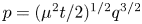 $p=(\mu ^2 t/2)^{1/2}q^{3/2}$, the far-field leading wave solution (2.21) can be rewritten as
 \begin{align} \eta_{lead}(r,\theta,t)&=\frac{2V_B}{3\sqrt{\rm \pi}}\left(\frac{2}{\mu^2 t}\right)^{1/2}r^{-{1/2}}\frac{{\mathit{Fr}}\cos\theta}{2(1-{\mathit{Fr}}\cos\theta)}\varOmega_1\left(\left(\frac{2}{\mu^2 t}\right)^{1/3}\left(r-t\right)\right)\nonumber\\ &\quad -\frac{2M_1(\theta)}{3\sqrt{\rm \pi}}\left(\frac{2}{\mu^2 t}\right)^{5/6}r^{-{1/2}}\frac{{\mathit{Fr}}\cos\theta}{2(1-{\mathit{Fr}}\cos\theta)}\varOmega_1'\left(\left(\frac{2}{\mu^2 t}\right)^{1/3}\left(r-t\right)\right)\nonumber\\ &\quad +\frac{M_2(\theta)}{3\sqrt{\rm \pi}}\left(\frac{2}{\mu^2 t}\right)^{7/6}r^{-{1/2}}\frac{{\mathit{Fr}}\cos\theta}{2(1-{\mathit{Fr}}\cos\theta)}\varOmega_1''\left(\left(\frac{2}{\mu^2 t}\right)^{1/3}\left(r-t\right)\right) +\cdots , \end{align}
where the function  $\varOmega _1(s)$ is defined as
 \begin{equation} \varOmega_1(s)=\frac{\displaystyle\int_0^\infty \cos\left(s p^{2/3}+\dfrac{1}{3}p^2\right) \textrm{d}p+\int_0^\infty \sin\left(s p^{2/3}+\dfrac{1}{3}p^2\right) \textrm{d}p}{2{\rm \pi}}. \end{equation}
In (2.22),  $V_B$ (see (B3)) is the volume enclosed by the bottom obstacle,
  $M_1(\theta )$ (see (B6)) is the ‘first moment of the bottom obstacle shape in the
  $\theta$ direction’ and
  $M_2(\theta )$ (see (B9)) is the ‘second moment of the bottom obstacle shape in the
  $\theta$ direction’. Similarly to the Lo & Liu (Reference Lo and Liu2017) findings for the 1DH case, in the far field, the leading wave generated by a moving bottom obstacle depends primarily on the volume enclosed by the obstacle. The exact shape of the obstacle, which shows up as the higher-order moments in (2.22), has only secondary effects that decay more rapidly in time. In this study, when plotting the far-field leading wave solution, only the first term in (2.22) is considered.
The far-field leading wave solution (2.22) reveals two important facts: first, regardless of the obstacle shape, the leading waves generated by a translating bottom obstacle evolve into the same shape due to frequency dispersion; second, to the leading order, the volume enclosed by the obstacle is directly proportional to the leading wave amplitude. Interestingly, these facts appear to hold true even in more complex configurations. For example, in the Sælevik, Jensen & Pedersen (Reference Sælevik, Jensen and Pedersen2009) 2-D laboratory experiments on water waves generated by subaerial landslides, the volume (or area in two dimensions) enclosed by the landslide was found to be the governing parameter for the leading wave amplitude. In the Paris et al. (Reference Paris, Okal, Guérin, Heinrich, Schindelé and Hébert2019) 2DH numerical simulations of the 2017 landslide tsunami event in Karrat Fjord, Greenland, the characteristic shape of the leading wave was found to be independent of the landslide volume, and increasing the landslide volume only seemed to increase the leading wave amplitude linearly.
The newly derived analytical solution (2.22) is unprecedented. Not only are assumptions on the obstacle shape function not needed in the derivation, but the new analytical solution also proves the above-mentioned observations to be true – i.e. the dependence of wave amplitude on the obstacle volume and the insensitivity to the exact obstacle shape – albeit in a highly idealised set-up.
The function  $\varOmega _1(s)$, (2.23), accounts for the exact shape of the far-field leading wave solution (2.22). It should be noted that the role of
  $\varOmega _1(s)$ in the 2DH bottom-obstacle-generated wave problem is similar to that of the function
  $T(p)$ presented in Kajiura (Reference Kajiura1963) and Mei et al. (Reference Mei, Stiassnie and Yue2005), who assumed a specific forcing function to derive analytical solutions for earthquake-generated tsunamis. In the classic 1DH far-field leading wave solutions (see e.g. Mei et al. Reference Mei, Stiassnie and Yue2005; Lo & Liu Reference Lo and Liu2017), the function that accounts for the exact wave shape is the Airy function, defined as
 \begin{equation} \textrm{Ai}(s)=\frac{\displaystyle\int_{0}^\infty \cos\left(sp+\dfrac{1}{3}p^3\right)\textrm{d}p}{\rm \pi}. \end{equation}
While the integral representation of the Airy function is well known, the  $p$-integrals in
  $\varOmega _1(s)$ are not of a common form, and will need to be examined more closely. The two functions are compared in figure 3. A main difference between
  $\varOmega _1(s)$ and
  $\textrm {Ai}(s)$ is that, while the leading wave in
  $\textrm {Ai}(s)$ has the largest amplitude, the trailing waves in
  $\varOmega _1(s)$ all have a larger amplitude than the leading wave. The leading wave in
  $\varOmega _1(s)$ has a maximum of
  $0.390$ at
  $s\simeq -0.467$, and the first trailing wave has a maximum of
  $0.568$ at
  $s\simeq -4.47$. On the other hand, the leading wave in
  $\textrm {Ai}(s)$ has a maximum of
  $0.536$ at
  $s\simeq -1.02$, and the first trailing wave has a maximum of
  $0.380$ at
  $s\simeq -4.83$. In both functions, the leading wave has the longest wavelength. That the trailing waves of
  $\varOmega _1(s)$ all have a larger amplitude than the leading wave is consistent with the Okal & Synolakis (Reference Okal and Synolakis2016) observation that the leading wave of a tsunami is not always the largest.


Differently from the 1DH problem, wave spreading in 2DH is accounted for by the addition of  $r^{-1/2}$ (which is a universal feature due to geometric spreading) and
  $\cos \theta$ in the solutions. In addition, the far-field leading wave in 2DH decays in time as
  $t^{-1/2}$, whereas that in 1DH decays in time as
  $t^{-1/3}$. Due to the term
  ${\mathit {Fr}}\cos \theta /2(1-{\mathit {Fr}}\cos \theta )$, water waves generated by a bottom obstacle moving in the
  $\theta =0$ direction always vanish near
  $\theta =\pm {\rm \pi}/2$. Since only subcritical obstacle speeds are considered, i.e.
  $0<{\mathit {Fr}}<1$, resonance does not occur for the far-field leading wave.
While the far-field leading wave solution (2.22) appears simple and universal, the trailing waves are not captured. Thus, little insight on the rest of the wave field can be gained without numerically evaluating the more representative integral-form solutions (2.17), (2.18), or (2.20). Lastly, it should be understood that the far-field leading wave solution relies on the leading-order frequency dispersion effect to manifest. The more frequency dispersive a problem is – that is, the larger  $\mu$ is or the deeper the water depth is in comparison to the obstacle length – the sooner the far-field leading wave solution becomes valid; vice versa. Therefore, in the shallow water limit,
  $\mu \to 0$, the far-field leading wave solution will never be reached. However, in such a limiting case, closed-form far-field solutions can be obtained, as will be discussed in § 2.4.
In a similar manner, the velocity solutions (normalised by  $\epsilon \sqrt {g d}$) for the far-field leading wave can also be derived (details can be found in the supplementary material). The results are
 \begin{gather}
u_{{lead}}(r,\theta,t)=\eta_{{lead}}(r,\theta,t)\cos\theta,
\quad
v_{{lead}}(r,\theta,t)=\eta_{{lead}}(r,\theta,t)\sin\theta,\notag\\
w_{{lead}}(r,\theta,t)=0,
\end{gather}
\begin{gather}
u_{{lead}}(r,\theta,t)=\eta_{{lead}}(r,\theta,t)\cos\theta,
\quad
v_{{lead}}(r,\theta,t)=\eta_{{lead}}(r,\theta,t)\sin\theta,\notag\\
w_{{lead}}(r,\theta,t)=0,
\end{gather}
where the expression for  $\eta _{{lead}}$ has been given in (2.22). Since the longest wave corresponding to
  $q=0$ travels the fastest to become the leading wave, the far-field leading waves are long waves. Consistent with the characteristics of long waves, the horizontal velocities of the far-field leading wave show no depth variation; i.e.
  $u_{{lead}}$ and
  $v_{{lead}}$ do not depend on
  $z$. In addition, the vertical velocity of the far-field leading wave is zero; i.e.
  $w_{{lead}}=0$. When the horizontal velocities are expressed in the
  $r$ and
  $\theta$ directions, related by
 \begin{equation} \left.\begin{gathered} R_{{lead}}(r,\theta,z,t)=u_{{lead}}(r,\theta,z,t)\cos\theta+v_{{lead}}(r,\theta,z,t)\sin\theta,\\ \varTheta_{{lead}}(r,\theta,z,t)={-}u_{{lead}}(r,\theta,z,t)\sin\theta+v_{{lead}}(r,\theta,z,t)\cos\theta ,\end{gathered}\right\} \end{equation}
the far-field leading wave velocity solutions become even more concise:
 \begin{equation} R_{{lead}}(r,\theta,t)=\eta_{{lead}}(r,\theta,t), \quad \varTheta_{{lead}}(r,\theta,t)=0,\quad w_{{lead}}(r,\theta,t)=0. \end{equation}
The newly derived velocity solutions such as (2.27a–c) are unprecedented. Traditionally, the initial flow velocities under a tsunami wave are assumed to be zero. While this assumption is reasonable for earthquake-generated tsunamis, it is not at all a reasonable assumption for landslide-generated tsunamis. Differently from the earthquake–wave generation process, the landslide–wave generation process is dynamic – the initial tsunami waves at the end of the wave generation process have non-zero initial flow velocities and must be considered. The far-field leading wave velocity solutions (2.27a–c) provide a simple means to link the free surface elevation to the flow velocities.
To check the accuracy of the far-field leading wave solutions, they should be compared with the complete solutions. In order to plot the complete integral-form solutions, an obstacle shape must be specified. As a reference shape in this study, we consider a radially symmetric Gaussian-shaped obstacle whose characteristic length is four times its standard deviation
 \begin{equation} B_0(r)=\textrm{e}^{{-}8r^2}. \end{equation}
For  ${\mathit {Fr}}=0.5$ and
  $\mu =0.3$, the wave fields at
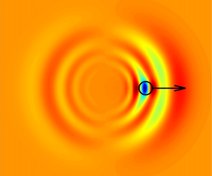
  $t=2,6,10$ are compared in figure 4. The trapped wave, which follows the obstacle and is omitted in the asymptotic solutions, can be clearly identified in the complete solutions near
  $x=1,3,5$ along the
  $x$-axis, at
  $t=2,6,10$, respectively. The free waves manifest as rings of waves that propagate radially outwards. Qualitatively, the far-field leading wave solution, theoretically accurate only for large
  $r$ and near
  $r=t$, indeed appears to capture well the overall wave characteristics near the leading wave.

Figure 4. The free surface elevations predicted by the linear and fully dispersive analytical solutions at three different times, with  ${\mathit {Fr}}=0.5$,
  $\mu =0.3$ and the Gaussian-shaped
  $B_0$ given in (2.28). (a–c) The complete integral-form solution (2.18); (d–f) the first term of the far-field leading wave solution (2.22), accurate for large
  $r$ and near
  $r=t$ for (a,d)
  $t=2$; (b,e)
  $t=6$; (c,f)
  $t=10$.
Taking a closer look, we plot the wave profiles in four different  $\theta$ directions in figure 5. The discrepancy can now be seen more clearly: while the leading wave near
  $r=t$ quickly converges to the far-field leading wave solution, the trailing waves do not. Hence, it is consistent with the asymptotic approximations made in the solution process – the closed-form far-field leading wave solution (2.22) is valid only in the far field (where
  $r$ is large) and near the leading wave (where
  $r\simeq t$). In this example,
  $r\simeq 6$ appears to be sufficiently large.

Figure 5. The free surface elevations predicted by the LFD analytical solutions plotted along four different directions at three different times, with  ${\mathit {Fr}}=0.5$,
  $\mu =0.3$ and the Gaussian-shaped
  $B_0$ given in (2.28): (a–d)
  $t=2$; (e–h)
  $t=6$; (i–l)
  $t=10$ for (a,e,i)
  $\theta =0$; (b,f,j)
  $\theta ={\rm \pi} /4$; (c,g,k)
  $\theta =3{\rm \pi} /4$; (d,h,l)
  $\theta ={\rm \pi}$. Circles, numerically integrated complete solution (2.18); dashed line, the first term of the far-field leading wave solution (2.22), accurate for large
  $r$ and near
  $r=t$.
To see how well the far-field leading wave velocity solutions (2.25a–c) compare with the complete integral-form solutions (expressions are shown in the supplementary material), the solutions at  $t=6$ are plotted in figure 6. It can be seen that, qualitatively, the far-field leading wave solutions indeed agree with the complete solutions, in the far field (large
  $r$), near the leading wave (near
  $r=t$), and away from the trapped wave (near
  $x={\mathit {Fr}} t$). The far-field horizontal velocity in the
  $\theta$ direction is derived to be zero – this feature starts to manifest in the complete velocity solutions at
  $t=6$.

Figure 6. The flow velocities predicted by the LFD analytical solutions at  $t=6$, with
  ${\mathit {Fr}}=0.5$,
  $\mu =0.3$ and the Gaussian-shaped
  $B_0$ given in (2.28). To enhance legibility, velocities near the bottom obstacle or the origin, where the asymptotic solutions are not applicable, are not shown. The corresponding free surface elevations are also plotted in the background. (a) The complete velocity solutions (shown in the supplementary material) at the still water surface
  $z=0$; (b) the far-field leading wave velocity solutions (2.27a–c), accurate for large
  $r$ and near
  $r=t$.
2.4. Shallow water solutions, $\mu \to 0$

As mentioned previously, the far-field leading wave solution relies on the leading-order frequency dispersion effect to manifest. In the shallow water limit,  $\mu \to 0$, the far-field leading wave solution will never be reached. Due to the lack of frequency dispersion (and thus the waves do not change shape as they propagate), the shape effect of the bottom obstacle is always present – each differently shaped obstacle generates differently shaped waves. Nonetheless, the shallow water limit allows for significant simplification of the analytical solutions. As a result, the most basic wave solutions can be obtained, particularly suitable for providing scaling relations between the bottom obstacle and the generated waves. By taking the limit of the LFD far-field solution (2.20) as
  $\mu \to 0$, the far-field solution in shallow water becomes
 \begin{align} \eta_{{far}}&= \frac{1}{\sqrt{2{\rm \pi}}}r^{-{1/2}}\frac{{\mathit{Fr}}\cos\theta}{2(1-{\mathit{Fr}}\cos\theta)}\int_0^\infty \widetilde{\overline{B_0}}(q,\theta)q^{1/2} \exp\left({\textrm{i}\left(q(r-t)-\frac{\rm \pi}{4}\right)}\right)\textrm{d}q\nonumber\\ &\quad +\frac{1}{\sqrt{2{\rm \pi}}}r^{-{1/2}}\frac{{\mathit{Fr}}\cos\theta}{2(1-{\mathit{Fr}}\cos\theta)}\int_0^\infty \widetilde{\overline{B_0}}(q,{\rm \pi}+\theta)q^{1/2} \exp\left({-\textrm{i}\left(q(r-t)-\frac{\rm \pi}{4}\right)}\right)\textrm{d}q . \end{align}
The integrands are simpler in this case and closed-form expressions are available for specific bottom obstacle shape functions  $B_0$.
Here, we derive the solutions for the reference Gaussian-shaped obstacle, (2.28), which is a radially symmetric obstacle shape function where  $B_0(x,y)=B_0(r)$;
  $\widetilde {\overline {B_0}}$ can then be simplified to
 \begin{align} \widetilde{\overline{B_0}} & =\frac{1}{2{\rm \pi}}\int_{-\infty}^\infty\int_{-\infty}^\infty B_0(x,y)\exp({-\textrm{i}kx})\exp({-\textrm{i}ly}) \,\textrm{d}\kern0.7pt x\,\textrm{d}y\nonumber\\ &=\frac{1}{2{\rm \pi}}\int_{0}^\infty\int_{0}^{2{\rm \pi}} B_0(r)\exp({-\textrm{i}qr\cos(\theta-\psi)})r\,\textrm{d}\theta \,\textrm{d}r \nonumber\\ &=\frac{1}{2{\rm \pi}}\int_{0}^\infty B_0(r) r \int_{0}^{2{\rm \pi}}\exp({-\textrm{i}qr\cos(\theta-\psi)})\,\textrm{d}\theta \, \textrm{d}r\nonumber\\ &=\frac{1}{2{\rm \pi}}\int_{0}^\infty B_0(r) r \int_{0}^{2{\rm \pi}}\exp({-\textrm{i}qr\cos\alpha})\,\textrm{d}\alpha \,\textrm{d}r\nonumber\\ &=\int_0^\infty B_0(r)r\textrm{J}_0(qr)\,\textrm{d}r=\mathcal{H}_0\{B_0(r)\}, \end{align}
where  $\textrm {J}_n(s)$ is the order-
 $n$ Bessel function of the first kind and
  $\mathcal {H}_n\{\,f\}$ denotes the order-
 $n$ Hankel transform of the function
  $f$. The expression for the Bessel integral
  $\textrm {J}_0(qr)=\int _0^{2{\rm \pi} }\exp ({-\textrm {i}qr\cos \alpha })\,\textrm {d}\alpha /2{\rm \pi}$ is used in the above equation.
For a real-valued obstacle shape function  $B_0$,
  $\mathcal {H}_0(B_0)$ is also real. The far-field solution (2.29) can then be simplified for a radially symmetric obstacle as
 \begin{align} \eta_{{far}} =\frac{1}{\sqrt{\rm \pi}}\frac{{\mathit{Fr}}\cos\theta}{2(1-{\mathit{Fr}}\cos\theta)}r^{-{1/2}}\int_0^\infty\mathcal{H}_0\{B_0\}q^{1/2} \left( \cos\left(q(r-t)\right)+\sin\left(q(r-t)\right)\right)\textrm{d}q. \end{align}
The  $q$-integral in the equation above can be evaluated in closed-form for the Gaussian-shaped obstacle (2.28). The far-field solution (2.31) then becomes
 \begin{equation} \eta_{{far}}(r,\theta,t)=\sqrt{\rm \pi}\frac{{\mathit{Fr}}\cos\theta}{2(1-{\mathit{Fr}}\cos\theta)}r^{-{1/2}}\varOmega_2(r-t), \end{equation}
which is a wave that propagates radially outwards at a normalised speed of one.
In (2.32),  $\varOmega _2(s)$ is defined as
 \begin{align} \varOmega_2(s)&= |s|^{3/2}\exp(-4s^2) \left[\textrm{I}_{5/4}\left(4s^2\right)-\textrm{I}_{1/4}\left(4s^2\right)+\frac{1}{8s^2}\textrm{I}_{1/4}\left(4s^2\right)\right.\nonumber\\ &\quad + \left.\text{sgn}(s)\left(\textrm{I}_{-{1/4}}\left(4s^2\right)-\textrm{I}_{3/4}\left(4s^2\right)\right)\right], \end{align}
where  $\textrm {I}_n(s)$ is the modified Bessel function of the first kind of order
  $n$, and
  $\text {sgn}(s)$ returns the sign of
  $s$. Similarly to
  $\varOmega _1(s)$, (2.23), in the dispersive leading wave solution, the function
  $\varOmega _2(r-t)=\varOmega _2(s)$ is a function of one variable only, and is the only term that accounts for the exact wave shape in (2.32). As shown in figure 7,
  $\varOmega _2(s)$ has the shape of the letter ‘N’, with a leading maximum of
  $0.213$ at
  $s\simeq 0.138$, which is followed by a minimum of
  $-0.0979$ at
  $s\simeq -0.437$. While a discontinuity exists at
  $s=0$ due to the division by
  $8s^2$ in (2.33), the limit as
  $s\to 0$ can be shown to be
  $\varOmega _2(s\to 0)=2^{1/4}/[8\varGamma (5/4)]\simeq 0.164$, where
  $\varGamma$ denotes the gamma function.

Figure 7. The  $\varOmega _2$ function defined in (2.33) plotted as a function of
  $s$.
$s$.
The shallow water far-field velocity solutions, valid for large  $r$, can be derived to be
 \begin{equation} u_{{far}}(r,\theta,t)=\eta_{{far}}(r,\theta,t)\cos\theta, \quad v_{{far}}(r,\theta,t)=\eta_{{far}}(r,\theta,t)\sin\theta. \end{equation}
Or, expressed in the  $r$ and
  $\theta$ directions:
 \begin{equation} R_{{far}}(r,\theta,t)=\eta_{{far}}(r,\theta,t), \quad \varTheta_{{far}}(r,\theta,t)=0. \end{equation}
 To check the accuracy of the shallow water far-field solution (2.32), we compare it against the numerically integrated complete solutions (2.18) in the shallow water limit where  $\mu \to 0$. For the Gaussian-shaped obstacle with
  ${\mathit {Fr}}=0.5$, the wave fields are compared in figure 8 at
  $t=2, 6, 10$. Due to the lack of frequency dispersion in shallow water, the waves do not deform. As a result, the trapped wave (which follows the obstacle) and the free waves (which propagate at a speed of one) can be easily identified. For a closer look, the results are plotted along four different directions in figure 9. Overall, the shallow water far-field solution quickly becomes accurate as
  $r$ increases. At
  $r\simeq 2$, it already captures parts of the free wave well; for
  $r\gtrsim 6$, it captures the free wave almost perfectly.
Figure 8. The free surface elevations predicted by the linear shallow water analytical solutions at three different times, with  ${\mathit {Fr}}=0.5$ and the Gaussian-shaped
  $B_0$ given in (2.28). (a–c) The complete integral-form solution (2.18) in the shallow water limit,
  $\mu \to 0$; (d–f) the far-field solution (2.32), accurate for large
  $r$ for (a,d)
  $t=2$; (b,e)
  $t=6$; (c,f)
  $t=10$.

Figure 9. The free surface elevations predicted by the linear shallow water analytical solutions plotted along four different directions at three different times, with  ${\mathit {Fr}}=0.5$ and the Gaussian-shaped
  $B_0$ given in (2.28). Circles, the complete integral-form solution (2.18) in the shallow water limit,
  $\mu \to 0$; dashed line, the far-field solution (2.32), accurate for large
  $r$: (a–d)
  $t=2$; (e–h)
  $t=6$; (i–l)
  $t=10$. (a,e,i)
  $\theta =0$; (b,f,j)
  $\theta ={\rm \pi} /4$; (c,g,k)
  $\theta =3{\rm \pi} /4$; (d,h,l)
  $\theta ={\rm \pi}$.
2.5. Trapped wave solutions
While this study primarily concerns the free wave  $\eta _+$, in this section we take a closer look at the trapped wave
  $\eta _{{\mathit {Fr}}}$, which was first identified in (2.17). If a moving coordinate is introduced,
  $\xi =x-{\mathit {Fr}} t$,
  $\eta _{{\mathit {Fr}}}(x,y,t)$ becomes independent of time and can be expressed as
 \begin{equation} \eta_{{\mathit{Fr}}}(\xi,y)={-}\frac{1}{2{\rm \pi}}\int_{-\infty}^{\infty}\int_{-\infty}^{\infty}\frac{\widetilde{\overline{B_0}}(k,l)}{\cosh(\mu q)}\frac{{\mathit{Fr}}^2\dfrac{k^2}{q^2}}{D^2-{\mathit{Fr}}^2\dfrac{k^2}{q^2}} \textrm{e}^{\textrm{i}k\xi}\textrm{e}^{\textrm{i}ly}\,\textrm{d}k \,\textrm{d}l. \end{equation}
Converted to polar coordinates (centred about the obstacle) using the substitutions  $\xi =r_{{\mathit {Fr}}}\cos \theta _{{\mathit {Fr}}}$,
  $y=r_{{\mathit {Fr}}}\sin \theta _{{\mathit {Fr}}}$,
  $k=q\cos \psi$, and
  $l=q\sin \psi$, the expression above becomes
 \begin{equation} \eta_{{{\mathit{Fr}}}}(r_{{\mathit{Fr}}},\theta_{{\mathit{Fr}}})={-}\frac{1}{2{\rm \pi}}\int_{0}^{2{\rm \pi}}\int_{0}^{\infty} \frac{q\widetilde{\overline{B_0}}(q,\psi)}{\cosh(\mu q)}\frac{{\mathit{Fr}}^2\cos^2\psi}{D^2-{\mathit{Fr}}^2\cos^2\psi} \exp({\textrm{i}qr_{{\mathit{Fr}}}\cos(\psi-\theta_{{\mathit{Fr}}})})\,\textrm{d}q\,\textrm{d}\psi. \end{equation}
Other than translating with the bottom obstacle, the trapped wave does not change in time. Therefore, it only needs to be numerically evaluated once.
For the example using a Gaussian-shaped obstacle with  ${\mathit {Fr}}=0.5$ and
  $\mu =0.3$, the wave field and the velocities of the trapped wave are plotted in figure 10, and the free surface elevations along four different transects are plotted in figure 11. Both the fully dispersive solutions and the shallow water solutions are shown in the figures. On the water surface, the bottom obstacle forces a significant depression, with a minimum of approximately
  $-0.131$ in the fully dispersive solution, and two minor elevations, with a maximum of approximately
  $0.027$ in the fully dispersive solution. The amplitudes decrease as the distance to the
  $x$-axis increases. To satisfy these translating water surface perturbations, non-zero flow velocities exist. By comparing the fully dispersive results with the shallow water results, it can be observed that the overall features of the wave and velocity fields are highly similar. However, frequency dispersion effects appear to smooth out the extrema – in the shallow water results, the water surface depression and the elevations all have slightly larger amplitudes.

Figure 10. The wave and velocity fields (at the still water surface  $z=0$) associated with the ‘trapped wave’ analytical solutions, with
  ${\mathit {Fr}}=0.5$,
  $\mu =0.3$ and the Gaussian-shaped
  $B_0$ given in (2.28). (a) The integral-form solutions (2.18), shown in the supplementary material, for the trapped wave only; (b) the integral-form solutions in the shallow water limit,
  $\mu \to 0$.

Figure 11. The free surface elevations associated with the ‘trapped wave’ analytical solutions plotted along four different transects, with  ${\mathit {Fr}}=0.5$,
  $\mu =0.3$ and the Gaussian-shaped
  $B_0$ given in (2.28): (a) along
  $y=0$; (b) along
  $y=0.2$; (c) along
  $y=0.4$; (d) along
  $y=0.6$. Circle and solid line, integral-form solution (2.18), for the trapped wave only; cross and dashed line, the integral-form solution in the shallow water limit,
  $\mu \to 0$.
2.6. Remarks on the analytical solutions
The above analytical analyses reveal that a translating bottom obstacle generates two types of waves – the free waves that propagate freely outwards and the trapped wave that stays on top of the obstacle. While the trapped wave is a steady-state solution (relative to the moving obstacle) that does not warrant further investigation, the free waves are more complex and require further attention.
The newly derived dispersive far-field leading wave solution (2.22) is a closed-form expression that accurately approximates the leading free waves in the far field ( $r\simeq t\simeq 6$ is found to be sufficiently large in the examples). The far-field leading wave solution indicates that, regardless of the bottom obstacle shape, due to frequency dispersion all leading waves evolve into the same shape (captured by the function
  $\varOmega _1$), and the volume enclosed by the bottom obstacle is directly proportional to the wave amplitude. These findings are of practical value, as they justify fixing an obstacle shape in laboratory experiments or numerical simulations, and allow the results from different studies to be generalised. In addition, the far-field leading wave flow velocities are given in (2.27a–c), which shows that the leading waves spread radially outwards in the far field. The velocity solutions such as (2.27a–c) provide a simple means to relate the free surface elevation to the flow velocities, on which information is often missing in tsunami studies.
In a nearly non-dispersive problem, an unphysically large distance (which approaches infinity in the non-dispersive limit) may be needed for the far-field leading wave solution to become valid. In such a situation, the shallow water far-field solution (2.29) is a more accurate model for describing the free waves in the far field ( $r\simeq 6$ is found to be sufficiently large in the examples). The non-dispersive free waves are N-shaped (as described by the function
  $\varOmega _2$, plotted in figure 7), which are led by a crest in the downwind direction (
 $-{\rm \pi} /2<\theta <{\rm \pi} /2$) and are led by a trough in the upwind direction (
 ${\rm \pi} /2<\theta <3{\rm \pi} /2$). The corresponding velocities are given in (2.35a,b), which shows that the free waves spread radially outwards in the far field. Although the Gaussian shape (2.28) is assumed in deriving the shallow water solutions, this act can be justified by the far-field leading wave solution (2.22), which states that the differences in obstacle shapes have no impacts on the leading wave asymptotically.
Similarly to Okada's model (Okada Reference Okada1985; see the discussion in § 1) for linking the parameters of an earthquake to the resulting seafloor displacement, and consequently the water surface displacement caused by the seafloor displacement, the closed-form asymptotic solutions (2.22) and (2.29) provide a means for linking the parameters of a submarine landslide (i.e. a translating bottom obstacle) to the water waves it generates. In addition, flow velocities can be calculated from (2.27a–c) or (2.35a,b). These asymptotic solutions can be used as the initial conditions for a tsunami propagation model of choice, which can propagate the landslide-generated leading waves into a larger domain with complex bathymetry. However, the idealisations assumed in the analytical derivations do not approximate reality well. For example, both a constant water depth and a suddenly moving bottom obstacle are assumed, neither of which holds true for a submarine landslide. Hence, extensive empirical tuning is still needed to construct an operational landslide tsunami generation model. Some numerical investigations will be demonstrated in § 3.
3. Numerical investigations
In § 2, both complete integral-form analytical solutions and closed-form asymptotic solutions have been derived for small-amplitude water waves generated by a bottom obstacle translating at a subcritical speed. While the analytical solutions reveal the scaling relations and the overall wave characteristics of this wave generation and evolution problem, they are necessarily limited by the small-amplitude assumption. As a result, nonlinear effects are not captured. In addition, simple mathematical expressions can be found only for a bottom obstacle that suddenly starts moving at a constant speed, essentially corresponding to an infinitely large initial acceleration; the effects due to the bottom obstacle's acceleration and deceleration cannot be examined using the present analytical approach.
To complement and verify the analytical solutions derived in § 2, in this section we employ numerical methods to solve five different sets of long-wave equations. The long-wave models to consider include: the linear shallow water wave equations (LSWE, which is linear and non-dispersive, with a truncation error of  $O(\epsilon ,\mu ^2)$), the linear and weakly dispersive wave model (LWD, with a truncation error of
  $O(\epsilon ,\mu ^4)$), the nonlinear shallow water wave equations (NSWE, which is nonlinear and non-dispersive, with a truncation error of
  $O(\mu ^2)$), the weakly nonlinear and weakly dispersive wave model (WNWD, with a truncation error of
  $O(\epsilon \mu ^2,\mu ^4)$) and the fully nonlinear and weakly dispersive wave model (FNWD, with a truncation error of
  $O(\mu ^4)$). The last two, WNWD and FNWD, are commonly referred to as ‘Boussinesq-type’ long-wave models. More detailed information on long-wave equations can be found in, e.g. Wei et al. (Reference Wei, Kirby, Grilli and Subramanya1995), Lynett & Liu (Reference Lynett and Liu2002) and Mitsotakis (Reference Mitsotakis2009).
Robust numerical methods for solving these long-wave equations are nowadays considered well known (see e.g. Toro Reference Toro2001; Li & Raichlen Reference Li and Raichlen2002; Wei, Mao & Cheung Reference Wei, Mao and Cheung2006; Shiach & Mingham Reference Shiach and Mingham2009; Kazolea et al. Reference Kazolea, Delis, Nikolos and Synolakis2012; Shi et al. Reference Shi, Kirby, Harris, Geiman and Grilli2012; Dutykh & Kalisch Reference Dutykh and Kalisch2013; Zhou, Zhan & Li Reference Zhou, Zhan and Li2016; Hatland & Kalisch Reference Hatland and Kalisch2019). Therefore, detailed descriptions of the numerical models need not be shown here. Interested readers are referred to the supplementary material. Once again, we emphasise that while both the complete integral-form analytical solutions and the numerical solvers can be applied to examine the critical and supercritical cases where  ${\mathit {Fr}}\geqslant 1$, in this study we keep a clear focus on the subcritical case where
  $0<{\mathit {Fr}}<1$.
Typically, to model a long-wave problem, one employs just one set of long-wave equations and develop a numerical solver for it. However, in this study, we utilise the different sets of long-wave equations to study the effects due to nonlinearity alone, frequency dispersion alone, and nonlinear frequency dispersion. For the same wave problem, comparing the results predicted by the different long-wave models enables the isolation of each of these effects. For example, comparing the LSWE results with the NSWE results reveals the effects due to nonlinearity alone; comparing the LSWE results with the LWD results reveals the effects due to frequency dispersion alone; comparing the NSWE results or the LWD results with the WNWD results or the FNWD results reveals the effects due to nonlinear frequency dispersion. Lynett & Liu (Reference Lynett and Liu2002) employed such an approach to study bottom-obstacle-generated waves in 1DH; in this study, we adopt this approach to study bottom-obstacle-generated waves in 2DH, with a focus on examining the deviations from the linear analytical solutions.
3.1. Nonlinear effects
First and foremost, under the same idealised configuration consisting of a solid bottom obstacle translating at a constant speed in constant water depth, what are the effects of nonlinearity and how do the results deviate from the linear analytical solution? Two classes of nonlinear effects are examined: the non-dispersive nonlinear effects and the dispersive nonlinear effects. The non-dispersive nonlinear effects, accounted for purely by the  $O(\epsilon )$ terms in the long-wave equations, can be isolated by comparing the NSWE results with the LSWE results. The dispersive nonlinear effects, accounted for by the interplay between the
  $O(\epsilon )$ terms, the
  $O(\mu ^2)$ terms and the cross-terms (if available) in the long-wave equations, can be isolated by comparing the FNWD or WNWD results with the LWD results.
To demonstrate these effects, we shall consider the same example used throughout this study, with  ${\mathit {Fr}}=0.5$,
  $\epsilon =0.3$,
  $\mu =0.3$ and the Gaussian-shaped
  $B_0$ given in (2.28); fairly large
  $\epsilon =0.3$ and
  $\mu =0.3$ are intentionally chosen to highlight the nonlinear effects and the frequency dispersion effects, respectively. Of course, by increasing the values of
  $\epsilon$ and
  ${\mathit {Fr}}$, nonlinearity can be further strengthened. Here, we pick just one example to demonstrate the characteristics of the nonlinear effects.
Let us examine the non-dispersive results first. The numerical results predicted by LSWE, NSWE and the far-field LSWE asymptotic solution are compared in figure 12(a–c) and figure 13(a–d) at  $t=10$. It can be observed that the non-dispersive results all demonstrate similar characteristics: N-shaped leading waves consisting of an elevation and a depression propagate radially outwards. However, the wave shapes are different due to non-dispersive nonlinear effects. Figure 13 shows that non-dispersive nonlinear effects steepen the wavefronts, resulting in more stretched and tilted waves.

Figure 12. The free surface elevations predicted by different wave models at  $t=10$, with
  ${\mathit {Fr}}=0.5$,
  $\epsilon =0.3$,
  $\mu =0.3$ and the Gaussian-shaped
  $B_0$ given in (2.28). (a) LSWE; (b) NSWE; (c) the far-field shallow water solution (2.32), accurate for large
  $r$; (d) LWD; (e) WNWD; (f) the first term of the far-field leading wave solution (2.22), accurate for large
  $r$ and near
  $r=t$.

Figure 13. The free surface elevations predicted by different wave models plotted along four different directions at  $t=10$, with
  ${\mathit {Fr}}=0.5$,
  $\epsilon =0.3$,
  $\mu =0.3$ and the Gaussian-shaped
  $B_0$ given in (2.28). (a–d) The non-dispersive models, in which the solid lines denote the LSWE results, the dash-dot lines denote the NSWE results and the dashed lines denote the far-field shallow water solution (2.32), accurate for large
  $r$. (e–h) The dispersive models, in which the solid lines denote the LWD results, the dash-dot lines denote the WNWD results, the dotted lines denote the FNWD results and the dashed lines denote the first term of the far-field leading wave solution (2.22), accurate for large
  $r$ and near
  $r=t$. (a,e)
  $\theta =0$; (b,f)
  $\theta ={\rm \pi} /4$; (c,g)
  $\theta =3{\rm \pi} /4$; (d,h)
  $\theta ={\rm \pi}$.
Interestingly, since bottom-obstacle-generated waves are directional, i.e. they have different amplitudes in different directions, nonlinearity is not globally important within the same problem. Specifically, as revealed by the far-field LSWE asymptotic solution (2.32) and figure 13, water waves in the upwind direction (i.e.  ${\rm \pi} /2 <\theta <3{\rm \pi} /2$, opposite the obstacle's direction of travel) have much smaller amplitudes than those in the downwind direction (i.e.
  $-{\rm \pi} /2<\theta <{\rm \pi} /2$, in the obstacle's direction of travel). Therefore, although nonlinear effects are significant in the downwind direction in this example, as revealed by the significant deviations of the NSWE results from the LSWE results in figure 13(a,b), they are not significant in the upwind direction, as revealed by the good performance of LSWE in figure 13(c,d). This observation suggests that in estimating the nonlinearity of bottom-obstacle-generated waves, a direction of interest must also be specified. Furthermore, due to the radial spreading in 2DH, wave amplitudes continue to decrease as the waves spread outwards; an initially nonlinear wave field will eventually become linear enough to be approximated by the linear wave theory.
Next, we examine the dispersive results. The numerical results predicted by LWD, WNWD and the far-field leading wave solution are compared in figures 12(d–f) and figure 13(e–h) at  $t=10$. The wave fields appear highly similar, and only minor differences in the trailing waves can be seen. A closer inspection in four select directions, i.e. figure 13, shows the differences more clearly. Due to frequency dispersion, the leading waves all assume similar shapes and resemble the linear far-field leading wave solution (2.22); dispersive nonlinear effects seem to only increase the wave height of the leading waves. In this example, the linear models (i.e. LWD and the far-field leading wave solution) perform well except in the
  $\theta =0$ direction, where wave nonlinearity is the strongest. In contrast to the non-dispersive results, due to frequency dispersion, the overall wave nonlinearity is further decreased, making linear dispersive wave models more widely applicable.
Lastly, we note that both the WNWD results and the FNWD results are shown in figure 13. Nearly no discrepancy is observed. This is not surprising as differences between these two wave models are expected only in circumstances with strong nonlinearity, such as wave shoaling and wave breaking. In our 2DH problem with a local source, the overall wave nonlinearity actually decreases as the waves spread radially outwards – the difference between the WNWD results and the FNWD results is negligible, at least for the leading waves. Therefore, in this study, WNWD is used as the representative nonlinear and frequency dispersive long-wave model. From a practical point of view, this is desirable, since WNWD is computationally more efficient, and FNWD suffers from potential instability issues (see e.g. Madsen & Fuhrman Reference Madsen and Fuhrman2020). We further remark that no significant difference between the leading waves predicted by WNWD and those predicted by FNWD was observed in the numerous simulations performed in Lo (Reference Lo2018), where the parameter range tested was 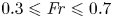 $0.3\leqslant {\mathit {Fr}}\leqslant 0.7$,
  $0.01\leqslant \epsilon \leqslant 0.3$ and
  $0.01\leqslant \mu \leqslant 0.3$.
3.2. Obstacle shape effects
The linear and dispersive far-field leading wave solution (2.22) indicates that due to frequency dispersion, all leading waves regardless of the bottom obstacle shape eventually evolve to have the same shape, but with different amplitudes. On the other hand, the linear and non-dispersive shallow water far-field solution (2.29) indicates that the non-dispersive free waves assume an N-shape and spread radially outwards without changing shape. Due to the lack of frequency dispersion, the wave shape is necessarily tied to the obstacle shape. In this section, the numerical solvers shall be utilised to see how nonlinear effects change these findings based on the linear analytical solutions. In addition, how sensitive the wave shape is to the obstacle shape in the non-dispersive limit will also be discussed.
In the numerical investigation, five different smooth and radially symmetric obstacle shapes are considered: the Gaussian shape that has been introduced in (2.28), the cubic exponential shape, the quartic exponential shape, the secant shape and the secant squared shape. The mathematical definitions of these five shapes are listed in table 1, and the five shapes are plotted in figure 14 as functions of  $r$. These five obstacle shapes have the same maximum height and enclose the same amount of volume. As can be seen from figure 14, the five different shapes can be regarded as having different characteristic steepness. The quartic exponential shape has the steepest face, the cubic exponential shape has the second steepest face, the Gaussian shape has the median steepness, the secant squared shape has the second mildest face and the secant shape has the mildest face.
Figure 14. The five smooth and radially symmetric bottom obstacle shapes considered in this study plotted as functions of  $r$. The five different shapes have the same maximum height and enclose the same amount of volume, and their definitions are listed in table 1. Solid line, the Gaussian shape; dash-dot line, the cubic exponential shape; dotted line, the quartic exponential shape; circle, the secant shape; cross, the secant squared shape.
Table 1. The five different smooth bottom obstacle shape functions  $B_0$ plotted in figure 14. They all have the same maximum height and enclose the same amount of volume,
  $V_B={\rm \pi} /8$. Here,
  ${Ca}\simeq 0.915965$ is the Catalan constant;
  $\varGamma$ denotes the gamma function.

Firstly, let us consider the simplest scenario – the results predicted by LSWE using the five different shapes. For the same example with  ${\mathit {Fr}}=0.5$, the free surface elevations at
  $t=10$ in four select directions are plotted in figure 15(a–d). The overall wave characteristics appear insensitive to the obstacle shape – the free waves are N-shaped and propagate radially outwards at a speed of one. The characteristic steepness of the obstacle shape appears to only affect the extrema of the N-shaped waves – the steeper the obstacle face is, the larger the magnitudes of the extrema. It can also be observed that the milder the obstacle face is, the smoother and more stretched out the resulting waves are. Then, we include nonlinear effects – the NSWE results with
  $\epsilon =0.3$ are plotted in figure 15(e–h). The obstacle shape effects appear similar to those in the linear case.

Figure 15. The free surface elevations generated by bottom obstacles of different shapes and predicted by different wave models, plotted along four different directions at  $t=10$, with
  ${\mathit {Fr}}=0.5$,
  $\epsilon =0.3$ and
  $\mu =0.3$. The five different shapes are defined in table 1 and plotted in figure 14. Solid line, the Gaussian shape; dash-dot line, the cubic exponential shape; dotted line, the quartic exponential shape; circle, the secant shape; cross, the secant squared shape. In the top two rows, the dashed lines denote the far-field shallow water solution (2.29); in the bottom two rows, the dashed lines denote the first term of the far-field leading wave solution (2.22). (a–d) LSWE; (e–h) NSWE; (i–l) LWD; (m–p) WNWD. (a,e,i,m)
  $\theta =0$; (b,f,j,n)
  $\theta ={\rm \pi} /4$; (c,g,k,o)
  $\theta =3{\rm \pi} /4$; (d,h,l,p)
  $\theta ={\rm \pi}$.
From the comparisons for the non-dispersive cases, i.e. figure 15(a–h), we conclude that the obstacle shape effects are secondary. The obstacle shape does not appear to impact the overall wave characteristics. A difference in obstacle shape primarily introduces relatively small perturbations to the magnitudes of the extrema and the smoothness of the wave shape. Thus, we claim that the closed-form far-field LSWE solution (2.29), although derived for a Gaussian-shaped obstacle, can be used as the simplest scaling relation between a translating bottom obstacle and the water waves it generates, regardless of the exact obstacle shape.
Next, we consider the frequency dispersive cases. We first verify that the far-field leading waves are insensitive to the exact obstacle shape within the linear and dispersive framework. In figure 15(i–l), the LWD results with  $\mu =0.3$ and the far-field leading wave solution (2.22) are plotted. The leading waves due to the five different obstacle shapes indeed converge to the far-field leading wave solution (2.22). Then, we include nonlinear effects – the WNWD results with
  $\epsilon =\mu =0.3$ are plotted in figure 15(m–p). Somewhat surprisingly, even in the presence of nonlinear effects, the leading waves are still not very sensitive to the exact obstacle shape and appear to converge to the same shape. While some amplitude differences show in the results – steeper obstacle faces result in slightly larger wave amplitudes – the overall wave shapes are nearly identical. Consistent with the linear analytical solution (2.22), the findings from this numerical investigation suggest that in modelling the far-field leading waves generated by a translating bottom obstacle, it is more important to estimate its enclosed volume than to capture its exact shape.
3.3. Obstacle acceleration effects
Thus far in this study, the bottom obstacle is assumed to suddenly start travelling at a normalised constant speed  ${\mathit {Fr}}$ from a halt. This is done to facilitate the analyses – it makes the derivation of closed-form analytical solutions possible, and allows the motion of the bottom obstacle to be fully described with just one parameter,
  ${\mathit {Fr}}$. However, realistically, no objects can suddenly travel at a constant speed from a halt, as this would mean an infinitely large initial acceleration. Therefore, in this section, we shall employ the numerical solvers, which place no restrictions on the obstacle's motion, to investigate the effects due to the obstacle's acceleration.
To make the obstacle's motion as tractable and parametrisable as possible, we consider the simplest way to account for obstacle acceleration in our problem set-up: a new input parameter  $t_{acc}$ is introduced so that the bottom obstacle accelerates from a halt to a normalised constant speed
  ${\mathit {Fr}}$ over a duration of
  $t_{acc}$. The obstacle then continues travelling at the constant speed indefinitely. The case in which the obstacle suddenly starts travelling at a constant speed then corresponds to the limiting case where
  $t_{acc}\to 0$.
As a first step, we again consider the simplest scenario – the results predicted by LSWE with different acceleration times  $t_{acc}$. Snapshots of the wave fields at three different instants,
  $t=2$,
  $t=6$ and
  $t=10$, and with different acceleration times
  $t_{acc}\to 0$,
  $t_{acc}=1$ and
  $t_{acc}=2$, are shown in figure 16. The overall wave pattern appears similar: free waves propagate radially outwards, followed by the trapped wave that stays on top of the bottom obstacle.

Figure 16. The free surface elevations generated by an initially stationary Gaussian-shaped bottom obstacle accelerating for a duration of  $t_{acc}$ until it reaches the normalised constant speed
  ${\mathit {Fr}}=0.5$. The results are numerically simulated based on LSWE. (a–c) Instantaneous acceleration,
  $t_{acc}\to 0$; (d–f)
  $t_{acc}=1$; (g–i)
  $t_{acc}=2$. (a,d,g)
  $t=2$; (b,e,h)
  $t=6$; (c,f,i)
  $t=10$.
Since linear long waves do not deform when travelling freely in constant water depth, we expect a quasi-steady state to be reached by the outward-propagating free waves after some time, regardless of  $t_{acc}$. Specifically, in the far field, i.e. for a sufficiently large
  $r$, we expect the free waves to assume a fixed shape whose amplitude decays as
  $r^{-1/2}$ due to radial spreading, as suggested by the far-field shallow water solution (2.29). To check this hypothesis, we plot the free surface elevations for
  $t_{acc}=1$ in four select directions at different instants in figure 17. In addition, the
  $r^{-1/2}$ decay rate is compared with the actual decay rate of the leading wave. Our hypothesis appears true: regardless of the acceleration time
  $t_{acc}$, the free waves eventually assume a fixed shape whose amplitude decays as
  $r^{-1/2}$; that is, a quasi-steady state can be reached.

Figure 17. The free surface elevations generated by an initially stationary Gaussian-shaped bottom obstacle accelerating for a duration of  $t_{acc}=1$ until it reaches the normalised constant speed
  ${\mathit {Fr}}=0.5$. The results are numerically simulated based on LSWE and plotted along four different directions at five different times. Solid line,
  $t=6$; dash-dot line,
  $t=7$; dotted line,
  $t=8$; circle,
  $t=9$; cross,
  $t=10$. The dashed lines denote the
  $r^{-1/2}$ decay rate suggested by the far-field solution (2.29). Panels show (a)
  $\theta =0$; (b)
  $\theta ={\rm \pi} /4$; (c)
  $\theta =3{\rm \pi} /4$; (d)
  $\theta ={\rm \pi}$.
That a quasi-steady state can be reached by the free waves regardless of the bottom obstacle's acceleration time  $t_{acc}$ greatly simplifies the investigation on obstacle acceleration effects, at least in the linear shallow water limit. All that remains to be examined is how
  $t_{acc}$ changes the wave shape in comparison with the reference case where
  $t_{acc}\to 0$. The wave fields in figure 16 show that the larger the acceleration time
  $t_{acc}$ (i.e. the slower the acceleration), the smaller the wave height and the longer the wavelength. Similar findings on the effects of acceleration were obtained by others under different obstacle-generated wave configurations; e.g. Sue, Nokes & Davidson (Reference Sue, Nokes and Davidson2011), Whittaker et al. (Reference Whittaker, Nokes, Lo and Liu2017) and Romano et al. (Reference Romano, Di Risio, Molfetta, Bellotti, Pasquali, Sammarco, Damiani and De Girolamo2017, Reference Romano, Lara, Barajas, Di Paolo, Bellotti, Di Risio, Losada and De Girolamo2020). For a closer look, the free surface elevations predicted by LSWE with five different values of
  $t_{acc}$ are plotted in the top row of figure 18 in four select directions at
  $t=10$. The effects of
  $t_{acc}$ in the linear shallow water limit can now be clearly seen:
  $t_{acc}\to 0$ corresponds to the most extreme case with the largest wave height, and larger values of
  $t_{acc}$ result in smaller but longer waves.

Figure 18. The free surface elevations generated by an initially stationary Gaussian-shaped bottom obstacle ( $\epsilon =0.3, \mu =0.3$) accelerating for a duration of
  $t_{acc}$ until it reaches the normalised constant speed
  ${\mathit {Fr}}=0.5$. The results are numerically simulated based on different wave models and plotted along four different directions at
  $t=10$. Solid line, instantaneous acceleration,
  $t_{acc}\to 0$; dash-dot line,
  $t_{acc}=0.5$; dotted line,
  $t_{acc}=1$; circle,
  $t_{acc}=1.5$; cross,
  $t_{acc}=2$. (a–d) LSWE; (e–h) NSWE; (i–l) LWD; (m–p): WNWD. For (a,e,i,m)
  $\theta =0$; (b,f,j,n)
  $\theta ={\rm \pi} /4$; (c,g,k,o)
  $\theta =3{\rm \pi} /4$; (d,h,l,p)
  $\theta ={\rm \pi}$.
Except for a time shift, the  $t_{acc}=0.5$ results appear highly similar to the
  $t_{acc}\to 0$ results. That water waves generated by a sufficiently fast accelerating obstacle share similar characteristics regardless of the actual magnitude of acceleration is consistent with the Romano et al. (Reference Romano, Lara, Barajas, Di Paolo, Bellotti, Di Risio, Losada and De Girolamo2020) numerical experiments on landslide-generated tsunamis. This finding further simplifies the investigation on obstacle acceleration effects: the limiting case
  $t_{acc}\to 0$, for which analytical solutions are derived, can be regarded as the most extreme and thus the most conservative scenario. On the other hand,
  $t_{acc}\gg 0$ corresponds to a creeping obstacle motion, which is inefficient at generating water waves. In the limiting case where
  $t_{acc} \to \infty$, the free surface displacement is expected to be negligible and converge to the still water solution.
Next, we account for nonlinear effects. The NSWE results are shown in figure 18(e–h). The same findings still hold. However, as the waves can now steepen due to nonlinear effects, the free waves continuously deform in addition to decaying at the rate  $r^{-1/2}$. In addition, larger values of
  $t_{acc}$ result in smaller but longer waves, further reducing the importance of nonlinearity and increasing the applicability of linear wave models.
Frequency dispersion effects in the absence of nonlinearity can be examined by inspecting the LWD results, plotted in figure 18(i–l). Grossly simplifying the obstacle acceleration effects, due to frequency dispersion, the leading waves in the far field all appear to converge to the far-field leading wave solution (derived for  $t_{acc}\to 0$), except with different time shifts. Including both frequency dispersion effects and nonlinear effects, the WNWD results are plotted in figure 18(m–p). It can be seen that nonlinearity only seems to increase the wave heights slightly. Just like in the LWD results, the leading waves all appear to converge to the asymptotic solution but with different time shifts. To see how similar the wave fields due to different
  $t_{acc}$ are, snapshots of the wave fields predicted by WNWD are shown in figure 19 for
  $t_{acc}\to 0$,
  $t_{acc}=1$, and
  $t_{acc}=2$. The wave fields appear highly similar, further confirming the observation that obstacle acceleration effects are nearly negligible in the far field for dispersive water waves.

Figure 19. The free surface elevations generated by an initially stationary Gaussian-shaped bottom obstacle ( $\epsilon =0.3, \mu =0.3$) accelerating for a duration of
  $t_{acc}$ until it reaches the normalised constant speed
  ${\mathit {Fr}}=0.5$. The results are numerically simulated based on WNWD. (a–c) Instantaneous acceleration,
  $t_{acc}\to 0$; (d–f)
  $t_{acc}=1$; (g–i)
  $t_{acc}=2$. For (a,d,g)
  $t=2$; (b,e,h)
  $t=6$; (c,f,i)
  $t=10$.
3.4. Obstacle deceleration effects and the leading wave separation time, $t_{sep}$

Realistically, most moving objects eventually decelerate to a halt. Thus, in this section we seek to investigate the effects due the obstacle's deceleration. Again, meticulous considerations must be taken in order to make the obstacle's motion as tractable and parametrisable as possible. To allow for obstacle deceleration as an extension of existing work, we consider a bottom obstacle that accelerates over a duration of  $t_{acc}$ to reach a normalised constant speed
  ${\mathit {Fr}}$. The obstacle then travels at the constant speed for a duration of
  $t_{{\mathit {Fr}}}$, before decelerating to a halt over a duration of
  $t_{dec}$. To isolate obstacle deceleration effects from the acceleration effects, here we consider only the limiting case where
  $t_{acc}\to 0$. We shall show that if
  $t_{{\mathit {Fr}}}$ is larger than the ‘leading wave separation time’,
  $t_{sep}$, the leading waves become insensitive to
  $t_{dec}$.
The duration of the constant speed movement,  $t_{{\mathit {Fr}}}$, is expected to have significant impacts on the generated water waves, since it directly controls the forcing time. Each different value of
  $t_{{\mathit {Fr}}}$ results in a unique wave field, making any generalisation of the findings difficult or impossible. Nonetheless, for a sufficiently large
  $t_{{\mathit {Fr}}}$, i.e. for a sufficiently long forcing time, the leading waves are able to travel far enough ahead of the bottom obstacle to become separated free waves unaffected by the wave forcing. Thus, there should exist a separation time
  $t_{sep}$ such that the leadings waves generated by a moving bottom obstacle becomes insensitive to the obstacle's subsequent motion (such as deceleration, controlled by
  $t_{dec}$) for
  $t_{{\mathit {Fr}}}\geqslant t_{sep}$.
For linear long waves in constant water depth, analytical expressions for the leading wave separation time  $t_{sep}$ can be derived. Suppose at
  $t=0$, the obstacle suddenly starts moving at a normalised constant speed
  ${\mathit {Fr}}$ into the positive
  $x$ direction from the origin. The first ring of disturbance, which can be seen as the representative location of the leading waves, is immediately generated and propagates radially outwards at a normalised speed of one. Hence, the radius of the first disturbance ring can be denoted as
  $t$, whereas the
  $x$ coordinate of the obstacle can be denoted as
  ${\mathit {Fr}} t$. The distance between the bottom obstacle, located at
 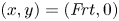 $(x,y)=({\mathit {Fr}} t,0)$, and the first disturbance ring in the
  $\theta$ direction, located at
  $(x,y)=(t\cos \theta ,t\sin \theta )$, can be calculated as
 \begin{equation} s=t\sqrt{(\cos\theta-{{\mathit{Fr}}})^2+\sin\theta^2}=t\sqrt{1-2{{\mathit{Fr}}}\cos\theta+{{\mathit{Fr}}}^2}. \end{equation}
Since the normalised characteristic wavelength is one, we assume the leading wave in the  $\theta$ direction to have sufficiently separated from the bottom obstacle when the normalised distance between the two is one; i.e.
  $s=1$ (alternately, an arbitrary separation distance can be specified). Consequently, the leading wave separation time can be expressed as
 \begin{equation} t_{sep}(\theta)=\frac{1}{\sqrt{1-2{{\mathit{Fr}}}\cos\theta+{{\mathit{Fr}}}^2}}. \end{equation}
Thus, the separation time  $t_{sep}$ is a function of the direction of interest,
  $\theta$. The leading waves in different directions require different amounts of time to separate from the bottom obstacle. While the leading wave in the
  $\theta ={\rm \pi}$ direction separates from the obstacle the soonest, the leading wave in the
  $\theta =0$ direction takes the longest time to separate from the obstacle:
  $t_{sep}(0)=1/(1-{\mathit {Fr}})$.
When the bottom obstacle decelerates after a sufficiently long forcing time, i.e.  $t_{{\mathit {Fr}}}\geqslant t_{sep}$, we expect the deceleration to have no effects on the leading waves, which have sufficiently separated from the obstacle already. To test the concept of the leading wave separation time
  $t_{sep}$ and the expression derived in (3.2), we specify
  $t_{{\mathit {Fr}}}=t_{sep}(0)=2$ in the same example with
  ${\mathit {Fr}}=0.5$, and plot the wave fields predicted by LSWE due to different deceleration times
  $t_{dec}$ in figure 20. The leading waves indeed appear to be unaffected by the obstacle's deceleration, as the trailing waves caused by the deceleration can never catch up.

Figure 20. The free surface elevations generated by a Gaussian-shaped bottom obstacle which suddenly starts moving at a normalised constant speed  ${\mathit {Fr}}=0.5$ for a duration of
  $t_{{\mathit {Fr}}}=t_{sep}(0)=2$, before decelerating to a halt over a duration of
  $t_{dec}$. The results are numerically simulated based on LSWE. (a–c) Instantaneous deceleration,
  $t_{dec}\to 0$; (d–f)
  $t_{dec}=1$; (g–i)
  $t_{dec}=2$. For (a,d,g)
  $t=2$; (b,e,h)
  $t=6$; (c,f,i)
  $t=10$.
The free surface elevations in four select directions are plotted in the first row of figure 21. In addition, the far-field shallow water solution (2.29) where the obstacle moves at a constant speed indefinitely are also shown. The results clearly show the leading wave to be unaffected by the obstacle's deceleration, and the far-field shallow water solution (2.29) can be used to accurately predict the leading waves regardless of the deceleration time  $t_{dec}$. The trailing waves, however, are affected. The limiting case
  $t_{dec}\to 0$ has the largest trailing waves, and larger values of
  $t_{dec}$ result in smaller but longer trailing waves. These trailing waves are originally trapped waves that follow the bottom obstacle. As the obstacle slows down, these trapped waves get released and become trailing waves. Therefore, in the reference case where the obstacle moves at a constant speed indefinitely, these trailing waves are absent. To account for nonlinear effects, the NSWE results are shown in figure 21(e–h). The findings remain unchanged.
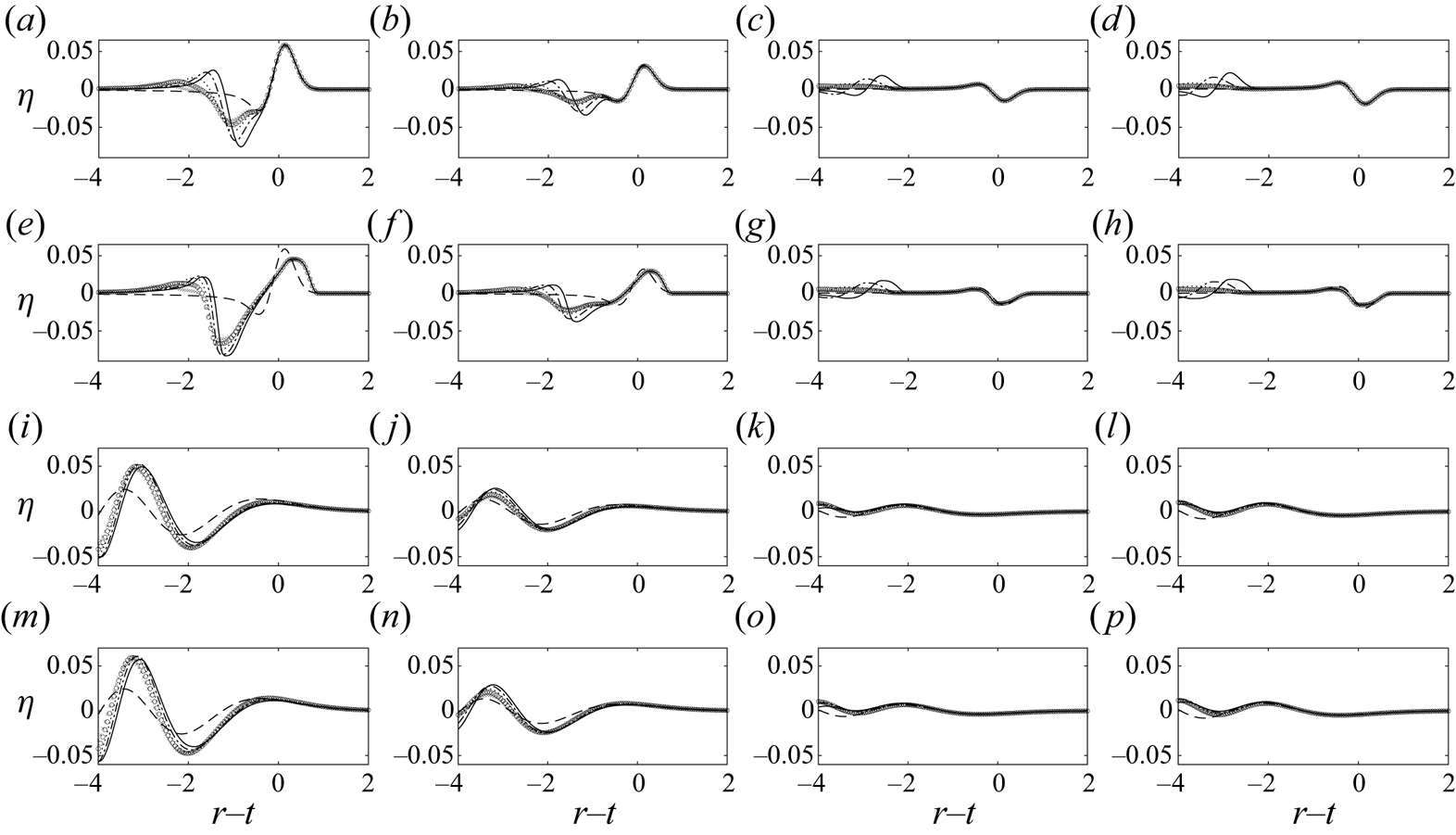
Figure 21. The free surface elevations generated by a Gaussian-shaped bottom obstacle ( $\epsilon =0.3$ and
  $\mu =0.3$) which suddenly starts moving at a normalised constant speed
  ${\mathit {Fr}}=0.5$ for a duration of
  $t_{{\mathit {Fr}}}=t_{sep}(0)=2$, before decelerating to a halt over a duration of
  $t_{dec}$. The results are plotted along four different directions at
  $t=10$. Solid line, instantaneous deceleration,
  $t_{dec}\to 0$; dash-dot line,
  $t_{dec}=0.5$; dotted line,
  $t_{dec}=1$; circle,
  $t_{dec}=1.5$; cross,
  $t_{dec}=2$. In the top two rows, the dashed lines denote the far-field shallow water solution (2.29) where the obstacle moves at a constant speed indefinitely; in the bottom two rows, the dashed lines denote the first term of the far-field leading wave solution (2.22) where the obstacle moves at a constant speed indefinitely. (a–d) LSWE; (e–h) NSWE; (i–l) LWD; (m–p) WNWD. For (a,e,i,m)
  $\theta =0$; (b,f,j,n)
  $\theta ={\rm \pi} /4$; (c,g,k,o)
  $\theta =3{\rm \pi} /4$; (d,h,l,p)
  $\theta ={\rm \pi}$.
To allow for frequency dispersion in the absence of nonlinearity, the LWD results are shown in figure 21(i–l). The results again appear to converge to some asymptotic form but with slight time shifts. However, this asymptotic form now differs from the far-field leading wave solution (2.22) where the obstacle moves at a constant speed indefinitely. Since frequency dispersion allows parts of the trailing waves to catch up with parts of the leading waves, whether additional trailing waves exist or not should have an impact on the overall wave shape. While additional trailing waves are generated when the obstacle slows down and releases the trapped waves, no additional trailing waves are generated in the reference case where the obstacle moves at a constant speed indefinitely. Thus, the leading waves are expected to assume different shapes in these two somewhat different cases. Nevertheless, we note that the far-field leading wave solution (2.22) still estimates well the wave height of the first wave, and a strong discrepancy in wave shape only shows in the  $\theta =0$ direction, where the additional trailing waves generated by the obstacle's deceleration are the closest to the leading waves.
To account for nonlinear frequency dispersion effects, the WNWD results are shown in figure 21(m–p). Once again, nonlinearity in the presence of frequency dispersion only seems to increase the wave amplitudes slightly. The findings based on the LWD results still hold. To see how similar the wave fields due to different  $t_{dec}$ are, snapshots of the wave fields predicted by WNWD are shown in figure 22 for
  $t_{dec}\to 0$,
  $t_{dec}=1$, and
  $t_{dec}=2$. The wave fields appear highly similar, further confirming the hypothesis that the leading waves are insensitive to the obstacle's deceleration if
  $t_{{\mathit {Fr}}}\geqslant t_{sep}$.

Figure 22. The free surface elevations generated by a Gaussian-shaped bottom obstacle ( $\epsilon =0.3$ and
  $\mu =0.3$) which suddenly starts moving at a normalised constant speed
  ${\mathit {Fr}}=0.5$ for a duration of
  $t_{{\mathit {Fr}}}=t_{sep}(0)=2$, before decelerating to a halt over a duration of
  $t_{dec}$. The results are numerically simulated based on WNWD. (a–c) Instantaneous deceleration,
  $t_{dec}\to 0$; (d–f)
  $t_{dec}=1$; (g–i)
  $t_{dec}=2$. For (a,d,g)
  $t=2$; (b,e,h)
  $t=6$; (c,f,i)
  $t=10$.
4. Concluding remarks
In this study, we investigated water waves generated by a bottom obstacle translating at a subcritical speed. New analytical solutions were derived using the LFD wave theory. An idealised configuration, consisting of a solid bottom obstacle that suddenly starts travelling at a constant speed in a constant water depth, was considered. With this configuration, complete integral-form solutions were obtained for both free surface elevation and flow velocities. The analytical solutions reveal two types of waves – the free waves that propagate outwards away from the source at the linear wave speed, and the trapped wave of a fixed shape that always stays on top of the bottom obstacle. Discontinuities exist in the integrands of the complete integral-form solutions. However, we showed these discontinuities to be either integrable based on the Cauchy principal value, or cancelled out by a component of identical magnitude and opposite sign. As a result, the integral-form solutions were numerically evaluated by carefully avoiding the discontinuities.
For a bottom obstacle travelling at a subcritical speed, the free waves it generates eventually propagate ahead of the obstacle to become the dominant waves. Asymptotic solutions in the far field, i.e. for a large distance  $r$ away from the origin (
 $r\simeq 6$ was found to be sufficient in the examples), were derived. The free waves were shown to propagate strictly radially outwards in the far field. For a Gaussian obstacle shape and in the shallow water limit, closed-form far-field solutions were obtained. The newly derived far-field shallow water solutions provide the simplest picture and scaling relations of water waves generated by a translating bottom obstacle: the free waves are N-shaped, propagate radially outwards, have different signs and amplitudes in different propagation directions, and maintain a fixed shape except with an amplitude decay rate of
  $r^{-1/2}$ due to radial spreading.
Another round of asymptotic approximation was performed on the far-field solutions to obtain the far-field leading wave solutions, accurate for large  $r$ and near the leading wave,
  $r\simeq t$ (
 $r\simeq t\simeq 6$ was found to be sufficient in the examples). The far-field leading wave solutions are in closed forms, and thus easy to use. Without the need to specify an obstacle shape, the newly derived far-field leading wave solutions show that, due to frequency dispersion, all leading waves eventually evolve to the same shape, which is insensitive to the exact shape of the obstacle. The volume enclosed by the obstacle has the strongest effect on the amplitude of the leading waves, whereas the exact shape of the obstacle has but secondary effects. This analytical finding is highly helpful, as it enables the generalisation of the results obtained from numerical simulations or laboratory experiments on bottom-obstacle-generated waves, in which a fixed obstacle shape must be specified in each realisation.
Numerical experiments were carried out to examine nonlinear effects. In the absence of frequency dispersion, nonlinear effects were found to steepen the wave fronts. Nonetheless, the overall wave pattern suggested by the analytical solutions remained unchanged: N-shaped waves, with different signs and amplitudes in different propagation directions, travel radially outwards, and their amplitudes decay due to radial spreading. In the presence of frequency dispersion, nonlinear effects only seemed to increase the wave amplitudes slightly. Since the free waves generated by a translating bottom obstacle are directional, i.e. the wave amplitudes are different in different propagation directions  $\theta$, nonlinearity may not be globally significant. The waves in the downwind direction (
 $-{\rm \pi} /2 <\theta <{\rm \pi} /2$) are always larger than the waves in the upwind direction (
 ${\rm \pi} /2 <\theta <3{\rm \pi} /2$). In addition, due to radial spreading, wave amplitudes decay continuously; initially large waves eventually decay to small-amplitude waves that can be accurately described by linear wave models. Similarly, obstacle shape effects were also investigated in the presence of nonlinearity. The overall wave shape was found to remain insensitive to the exact obstacle shape. Only small differences in wave amplitudes were observed. All in all, we found the linear analytical solutions to be effective tools for understanding and predicting the leading-order characteristics of the leading waves generated by a bottom obstacle translating at a subcritical speed.
Numerical solvers were also utilised to examine the effects due to the obstacle's acceleration. The obstacle was allowed to accelerate at a prescribed rate until a specified constant speed was reached. The numerical results based on LSWE indicated the existence of quasi-steady state solutions for the leading waves generated by an accelerating obstacle – the leading waves maintained a fixed shape in the far field, except for an amplitude decay rate of  $r^{-1/2}$. We found that a larger obstacle acceleration resulted in larger but shorter waves, and that as the initial acceleration increased, the generated waves appeared to converge to the limiting case with an infinitely large initial acceleration, i.e. the idealised configuration in which the bottom obstacle suddenly starts travelling at a constant speed. Therefore, the linear analytical solutions can be regarded as conservative estimates that predict the largest waves. Nonlinear effects and nonlinear frequency dispersion effects were also examined by comparing the numerical results predicted by the different long-wave models. The deviations from the linear wave model results were insignificant.
To examine the effects due to the obstacle's deceleration, the concept of leading wave separation time was proposed. The leading wave separation time is the time required for the leading waves to travel far enough away from the obstacle to become unaffected by the wave forcing. If the wave forcing duration is shorter than the leading wave separation time, all waves are affected by the obstacle's exact motion (such as acceleration and deceleration), and each different trajectory of the obstacle is expected to result in a different wave field, making attempts to generalise the results difficult. However, if the wave forcing duration is longer than the leading wave separation time, the leading waves are able to separate from the wave forcing and become free waves, which are insensitive to the obstacle's subsequent motion (such as deceleration). This hypothesis was successfully verified by numerical experiments, in which the obstacle travelled at a constant speed for a duration as long as the leading wave separation time, before decelerating at different rates to a halt. Obstacle deceleration indeed had negligible effects on the leading waves.
This study was primarily motivated by tsunamis generated by a submarine landslide. Realistically, the exact shape and the exact motion, let alone the exact material composition and properties, of a submarine landslide cannot be easily determined. While (almost) any shape and any motion can be used in numerical or laboratory experiments, their geophysical relevance cannot be verified. Furthermore, findings based on a specific experimental set-up can be difficult to generalise. To circumvent these difficulties, in this study we instead focused on a highly idealised configuration, in which the problem becomes parametrisable and closed-form analytical solutions are available. These analytical solutions – specifically, the dispersive far-field leading wave solution (2.22) and the shallow water far-field solution (2.29) – proved to be effective tools for predicting the leading-order wave characteristics. Similarly to Okada's model, which links the parameters of an earthquake to the resulting seafloor displacement, and consequently the water waves generated by the seafloor displacement, the closed-form asymptotic solutions (2.22) and (2.29), and their corresponding flow velocities (2.27a–c) and (2.35a,b), respectively, provide means for linking the parameters of a submarine landslide to the water waves it generates. Therefore, the newly derived analytical solutions have the potential to become the cornerstone of a theory-based model for quickly predicting the tsunamis generated by a submarine landslide.
Effects unaccountable by the linear analytical solutions can be numerically investigated, as demonstrated in § 3. It was shown that under certain conditions, the leading waves generated by a bottom obstacle remain insensitive to the exact shape and the exact motion of the obstacle. While this study is limited to constant water depth, it nonetheless provides the most basic scaling estimates and insights for bottom-obstacle-generated waves. To account for wave shoaling effects, variable water depths may be considered in a future study by adopting a semi-empirical approach. The ultimate objective is to construct an operational landslide tsunami generation model using a combination of analytical and empirical methods; this study has presented the essential ingredients.
Supplementary material
Supplementary material is available at https://doi.org/10.1017/jfm.2021.537.
Acknowledgements
The constructive communications with the anonymous referees and the Associate Editor are deeply appreciated.
Funding
The authors are thankful for the support from Cornell University, where this work was first started. P.H.-Y.L. acknowledges the ongoing financial support from the Ministry of Science and Technology of Taiwan (grant nos 108-2218-E-002-075 and 109-2221-E-002-094) and National Taiwan University. P.L.-F.L. acknowledges the support from the National Research Foundation, Prime Minister's Office, Singapore, under its Marine Science Research and Development Programme (award no. MSRDP-05), and from the Ministry of Education through a Tier 2 grant to the National University of Singapore.
Declaration of interests
The authors report no conflict of interest.
Appendix A. Discontinuities in the analytical solutions
Discontinuities exist in the analytical solutions derived in § 2. For example, in (2.18), i.e.
 \begin{align} \eta_{{{\mathit{Fr}}}}(r,\theta,t)&={-}\frac{1}{2{\rm \pi}}\int_{0}^{2{\rm \pi}}\int_{0}^{\infty}\frac{q\widetilde{\overline{B_0}}(q,\psi)}{\cosh(\mu q)}\frac{{\mathit{Fr}}^2\cos^2\psi}{D^2-{\mathit{Fr}}^2\cos^2\psi} \nonumber\\ &\quad \times\exp({-\textrm{i}q {\mathit{Fr}}(\cos\psi) t})\exp({\textrm{i}qr\cos(\psi-\theta)})\,\textrm{d}q\,\textrm{d}\psi , \end{align}
and
 \begin{align} \eta_{+}(r,\theta,t)&=\frac{1}{2{\rm \pi}}\int_0^{2{\rm \pi}}\int_0^\infty \frac{q\widetilde{\overline{B_0}}(q,\psi)}{\cosh(\mu q)} \left( \frac{{\mathit{Fr}}\cos\psi}{2(D-{\mathit{Fr}}\cos\psi)}\exp({-\textrm{i}q\,\textrm{D}t})\right.\nonumber\\ &\quad\left.-\frac{{\mathit{Fr}}\cos\psi}{2(D+{\mathit{Fr}}\cos\psi)}\exp({\textrm{i}q\,\textrm{D}t})\right) \exp({\textrm{i}qr\cos(\psi-\theta)})\,\textrm{d}q\,d\,\psi , \end{align}
discontinuities occur for  $D=\pm {\mathit {Fr}}\cos \psi$. Here, we show that these discontinuities are either integrable based on the Cauchy principal value or cancelled out by each other.
A.1. The trapped wave $\eta _{{\mathit {Fr}}}$

Firstly, we consider the trapped wave  $\eta _{{\mathit {Fr}}}$ in (A1). Discontinuities exist in the integrand when
  $D^2={\mathit {Fr}}^2\cos ^2\psi$, or
  $\cos \psi =\pm D/{\mathit {Fr}}$. Since
  $0\leqslant D(q) \leqslant 1$ and
  ${\mathit {Fr}}>0$,
  $\cos \psi =\pm D/{\mathit {Fr}}$ is possible only for
  $D(q)\leqslant {\mathit {Fr}}$.
For  $D(q)<{\mathit {Fr}}$, the four critical
  $\psi$ values are
 \begin{equation} \psi_1=\cos^{{-}1}(D/{\mathit{Fr}}), \quad \psi_2={\rm \pi}-\psi_1, \quad \psi_3={\rm \pi}+\psi_1, \quad \psi_4=2{\rm \pi}-\psi_1. \end{equation}
To analyse the behaviour of  $\eta _{{\mathit {Fr}}}$ near these four discontinuities, we break the integral solution into multiple parts:
 \begin{align} \eta_{{\mathit{Fr}}}(r,\theta,t)&={-}\frac{1}{2{\rm \pi}}\int_{0}^{\infty}\int_{0}^{2{\rm \pi}} G_{{\mathit{Fr}}}(q,\psi,r,\theta,t)\,\textrm{d}\psi \,\textrm{d}q \nonumber\\ &={-}\frac{1}{2{\rm \pi}}\lim_{\delta\to 0}\left\{\vphantom{\left.+\int_{0}^{\infty}\int_{\psi_4+\delta}^{2{\rm \pi}} G_{{\mathit{Fr}}} \,\textrm{d}\psi \,\textrm{d}q \right\}} \int_{0}^{\infty}\int_{0}^{\psi_1-\delta} G_{{\mathit{Fr}}}\,\textrm{d}\psi\,\textrm{d}q +\int_{0}^{\infty}\int_{\psi_1-\delta}^{\psi_1+\delta} G_{{\mathit{Fr}}} \,\textrm{d}\psi \,\textrm{d}q \right.\nonumber\\ &\quad +\int_{0}^{\infty}\int_{\psi_1+\delta}^{\psi_2-\delta} G_{{\mathit{Fr}}} \,\textrm{d}\psi \,\textrm{d}q +\int_{0}^{\infty}\int_{\psi_2-\delta}^{\psi_2+\delta} G_{{\mathit{Fr}}} \,\textrm{d}\psi \,\textrm{d}q\nonumber\\ &\quad +\int_{0}^{\infty}\int_{\psi_2+\delta}^{\psi_3-\delta} G_{{\mathit{Fr}}} \,\textrm{d}\psi \,\textrm{d}q +\int_{0}^{\infty}\int_{\psi_3-\delta}^{\psi_3+\delta} G_{{\mathit{Fr}}} \,\textrm{d}\psi \,\textrm{d}q\nonumber\\ &\quad +\int_{0}^{\infty}\int_{\psi_3+\delta}^{\psi_4-\delta} G_{{\mathit{Fr}}} \,\textrm{d}\psi \,\textrm{d}q +\int_{0}^{\infty}\int_{\psi_4-\delta}^{\psi_4+\delta} G_{{\mathit{Fr}}} \,\textrm{d}\psi \,\textrm{d}q\nonumber\\ &\quad \left.+\int_{0}^{\infty}\int_{\psi_4+\delta}^{2{\rm \pi}} G_{{\mathit{Fr}}} \,\textrm{d}\psi \,\textrm{d}q \right\}, \end{align}
where  $G_{{\mathit {Fr}}}(q,\psi ,r,\theta ,t)$ is used to denote the integrand in (A1).
The integral of interest is thus of the form
 \begin{align} I_*(r,\theta,t)&=\lim_{\delta\to 0}\int_{0}^{\infty}\int_{\psi_*-\delta}^{\psi_*+\delta} \frac{q\widetilde{\overline{B_0}}(q,\psi)}{\cosh(\mu q)}\frac{{\mathit{Fr}}^2\cos^2\psi}{D^2-{\mathit{Fr}}^2\cos^2\psi} \nonumber\\ &\quad \times\exp({-\textrm{i}q {\mathit{Fr}}(\cos\psi) t})\exp({\textrm{i}qr\cos(\psi-\theta)} )\,\textrm{d}\psi \,\textrm{d}q, \end{align}
where  $\psi _*$ denotes the critical values of
  $\psi$. Following an approach similar to the Lo & Liu (Reference Lo and Liu2017) analysis for 1DH problems, we use the Taylor series to expand each term in the integrand about
  $\psi =\psi _*$ to obtain
 \begin{align} I_*&=\lim_{\delta\to 0}\int_{0}^{\infty}\int_{\psi_*-\delta}^{\psi_*+\delta} \frac{q\widetilde{\overline{B_0}}(q,\psi_*)}{\cosh(\mu q)}\frac{{\mathit{Fr}}^2\cos^2\psi_*}{2{\mathit{Fr}}^2(\psi-\psi_*)\sin\psi_*\cos\psi_*}\nonumber\\ &\quad \times\exp({-\textrm{i}q {\mathit{Fr}}(\cos\psi_*) t}) \exp({\textrm{i}qr\cos(\psi_*-\theta)} )\,\textrm{d}\psi \,\textrm{d}q\nonumber\\ &=\int_{0}^{\infty}\frac{q\widetilde{\overline{B_0}}(q,\psi_*)}{\cosh(\mu q)}\frac{1}{2\tan\psi_*} \exp({-\textrm{i}q {\mathit{Fr}}(\cos\psi_*) t})\nonumber\\ &\quad \times\exp({\textrm{i}qr\cos(\psi_*-\theta)} )\,\textrm{d}q \left[ \lim_{\delta\to 0} \int_{\psi_*-\delta}^{\psi_*+\delta}\frac{1}{\psi-\psi_*} \textrm{d}\psi\right]\nonumber\\ &=\int_{0}^{\infty}\frac{q\widetilde{\overline{B_0}}(q,\psi_*)}{\cosh(\mu q)}\frac{1}{2\tan\psi_*} \exp({-\textrm{i}q {\mathit{Fr}}(\cos\psi_*) t})\nonumber\\ &\quad \times\exp({\textrm{i}qr\cos(\psi_*-\theta)} )\,\textrm{d}q \left[ \lim_{\delta\to 0} \int_{-\delta}^{\delta}\frac{1}{u} \textrm{d}u\right] . \end{align}
Based on the Cauchy principal value, the  $u$-integral is zero; hence the discontinuities at
  $\psi =\psi _*=\psi _1,\psi _2,\psi _3,\psi _4$ are integrable.
For  $D(q)={\mathit {Fr}}$ so that
  $\cos \psi =\pm 1$, only two critical values of
  $\psi$ exist:
  $\psi _1=0$, and
  $\psi _2={\rm \pi}$. Differently from the case for
  $D(q)<{\mathit {Fr}}$, an extra term needs to be kept in the Taylor series expansion of
  $D^2-{\mathit {Fr}}^2\cos ^2\psi$ to ensure a non-zero denominator. The integral of interest now simplifies to
 \begin{align} I_*&=\lim_{\delta\to 0}\int_{0}^{\infty}\int_{\psi_*-\delta}^{\psi_*+\delta} \frac{q\widetilde{\overline{B_0}}(q,\psi_*)}{\cosh(\mu q)}\frac{{\mathit{Fr}}^2\cos^2\psi_*}{{\mathit{Fr}}^2(\psi-\psi_*)^2\cos^2\psi_*}\nonumber\\ &\quad\times\exp({-\textrm{i}q {\mathit{Fr}}(\cos\psi_*) t} )\exp({\textrm{i}qr\cos(\psi_*-\theta)} )\,\textrm{d}\psi \,\textrm{d}q \nonumber\\ &=\int_{0}^{\infty}\frac{q\widetilde{\overline{B_0}}(q,\psi_*)}{\cosh(\mu q)} \exp({-\textrm{i}q {\mathit{Fr}}(\cos\psi_*) t}) \nonumber\\ &\quad\times\exp({\textrm{i}qr\cos(\psi_*-\theta)} )\,\textrm{d}q \left[\lim_{\delta\to 0} \int_{\psi_*-\delta}^{\psi_*+\delta}\frac{1}{(\psi-\psi_*)^2} \textrm{d}\psi\right]\nonumber\\ &=\int_{0}^{\infty}\frac{q\widetilde{\overline{B_0}}(q,\psi_*)}{\cosh(\mu q)}\frac{1}{2\tan\psi_*} \exp({-\textrm{i}q {\mathit{Fr}}(\cos\psi_*) t})\nonumber\\ &\quad \times\exp({\textrm{i}qr\cos(\psi_*-\theta)})\,\textrm{d}q \left[\lim_{\delta\to 0} \int_{-\delta}^{\delta}\frac{1}{u^2} \textrm{d}u\right] . \end{align}
The limit does not exist in this case. Hence, the discontinuities at  $\psi =\psi _*=\psi _1,\psi _2$ are not integrable for the case
  $D(q)={\mathit {Fr}}$. However, we will show in the next section that these discontinuities end up being cancelled out by identical components in the free wave
  $\eta _+$.
A.2. The free wave $\eta _+$

Next, we consider the free wave  $\eta _{{+}}$ in (A2). The free wave can be further decomposed into two parts:
  $\eta _+=\eta _{+,1}+\eta _{+,2}$ with
 \begin{align} \eta_{+,1}(r,\theta,t)&=\frac{1}{2{\rm \pi}}\int_0^{2{\rm \pi}}\int_0^\infty \frac{q\widetilde{\overline{B_0}}(q,\psi)}{\cosh(\mu q)} \frac{{\mathit{Fr}}\cos\psi}{2(D-{\mathit{Fr}}\cos\psi)}\nonumber\\ &\quad \times\exp({-\textrm{i}q\,\textrm{D}t}) \exp({\textrm{i}qr\cos(\psi-\theta)})\,\textrm{d}q\,\textrm{d}\psi\end{align}
and
 \begin{align} \eta_{+,2}(r,\theta,t)&={-}\frac{1}{2{\rm \pi}}\int_0^{2{\rm \pi}}\int_0^\infty \frac{q\widetilde{\overline{B_0}}(q,\psi)}{\cosh(\mu q)} \frac{{\mathit{Fr}}\cos\psi}{2(D+{\mathit{Fr}}\cos\psi)}\nonumber\\ &\quad \times\exp({\textrm{i}q\,\textrm{D}t}) \exp({\textrm{i}qr\cos(\psi-\theta)})\,\textrm{d}q\,\textrm{d}\psi . \end{align}
 For  $\eta _{+,1}$, discontinuities exist when
  $D={\mathit {Fr}}\cos \psi$, or
  $\cos \psi =D/{\mathit {Fr}}$. Again, since
  $0\leqslant D(q) \leqslant 1$ and
  ${\mathit {Fr}}>0$,
  $\cos \psi =D/{\mathit {Fr}}$ is possible only for
  $D(q)\leqslant {\mathit {Fr}}$. For
  $D(q)<{\mathit {Fr}}$, the two critical
  $\psi$ values are:
  $\psi _1=\cos ^{-1}(D/{\mathit {Fr}})$ and
  $\psi _4=2{\rm \pi} -\psi _1$. To analyse the behaviour of
  $\eta _{+,1}$ near these two discontinuities where
  $D={\mathit {Fr}}\cos \psi$, only the integral of the form
 \begin{align} I_{*,1}(r,\theta,t)&=\lim_{\delta\to 0}\int_{0}^{\infty}\int_{\psi_*-\delta}^{\psi_*+\delta} \frac{q\widetilde{\overline{B_0}}(q,\psi)}{\cosh(\mu q)} \frac{{\mathit{Fr}}\cos\psi}{2(D-{\mathit{Fr}}\cos\psi)}\nonumber\\ &\quad \times\exp({-\textrm{i}q {\mathit{Fr}}(\cos\psi_*) t}) \exp({\textrm{i}qr\cos(\psi-\theta)} )\,\textrm{d}\psi \,\textrm{d}q \end{align}
needs to be examined. Expanding each function of  $\psi$ in the integrand about
  $\psi =\psi _*$, keeping the first non-zero terms, and simplifying yields
 \begin{align} I_{*,1}&=\int_{0}^{\infty}\frac{q\widetilde{\overline{B_0}}(q,\psi_*)}{\cosh(\mu q)}\frac{1}{2\tan\psi_*} \exp({-\textrm{i}q {\mathit{Fr}}(\cos\psi_*) t}) \exp({\textrm{i}qr\cos(\psi_*-\theta)})\,\textrm{d}q\nonumber\\ &\quad \times \left[ \lim_{\delta\to 0} \int_{-\delta}^{\delta}\frac{1}{u} \textrm{d}u\right]. \end{align}
The result ends up the same as that for the trapped wave – the discontinuities at  $\psi =\psi _*=\psi _1,\psi _4$ are integrable since the principal value of the
  $u$-integral is zero.
For  $D(q)={\mathit {Fr}}$ so that
  $\cos \psi = 1$, only one critical
  $\psi$ value exists:
  $\psi _1=0$. Differently from the case for
  $D(q)<{\mathit {Fr}}$, an extra term needs to be kept in the Taylor series expansion of
  $D-{\mathit {Fr}}\cos \psi$ to ensure a non-zero denominator. The integral of interest simplifies to
 \begin{align} I_{*,1}&=\int_{0}^{\infty}\frac{q\widetilde{\overline{B_0}}(q,\psi_*)}{\cosh(\mu q)}\frac{1}{2\tan\psi_*} \exp({-\textrm{i}q {\mathit{Fr}}(\cos\psi_*) t}) \exp({\textrm{i}qr\cos(\psi_*-\theta)} )\,\textrm{d}q\nonumber\\ &\quad \times \left[\lim_{\delta\to 0} \int_{-\delta}^{\delta}\frac{1}{u^2} \textrm{d}u\right] , \end{align}
which again is the same as the result for the trapped wave – the limit does not exist and thus the discontinuity at  $\psi =\psi _*=\psi _1$ is not integrable for the case
  $D(q)={\mathit {Fr}}$. However, the sign difference between the trapped wave (A1) and
  $\eta _{+,1}$ (A8) should be noted. Although the discontinuity (A12) is not integrable, it gets cancelled out by an identical component in the trapped wave, i.e. (A7).
Similar analyses can be repeated for  $\eta _{+,2}$ in (A9). For
  $\eta _{+,2}$, discontinuities exist when
  $D=-{\mathit {Fr}}\cos \psi$, or
  $\cos \psi =-D/{\mathit {Fr}}$. Again, since
  $0\leqslant D(q) \leqslant 1$ and
  ${\mathit {Fr}}>0$,
  $\cos \psi =D/{\mathit {Fr}}$ is possible only for
  $D(q)\leqslant {\mathit {Fr}}$. For
  $D(q)<{\mathit {Fr}}$, the two critical
  $\psi$ values are:
  $\psi _2={\rm \pi} -\cos ^{-1}(D/{\mathit {Fr}})$ and
  $\psi _3={\rm \pi} -\cos ^{-1}(D/{\mathit {Fr}})$. The integral of interest is
 \begin{align} I_{*,2}(r,\theta,t)&=\lim_{\delta\to 0}\int_{0}^{\infty}\int_{\psi_*-\delta}^{\psi_*+\delta} \frac{q\widetilde{\overline{B_0}}(q,\psi)}{\cosh(\mu q)} \frac{{\mathit{Fr}}\cos\psi}{2(D+{\mathit{Fr}}\cos\psi)}\nonumber\\ &\quad \times\exp({\textrm{i}q {\mathit{Fr}}(\cos\psi_*) t}) \exp({\textrm{i}qr\cos(\psi-\theta)})\,\textrm{d}\psi \,\textrm{d}q\nonumber\\ &={-}\int_{0}^{\infty}\frac{q\widetilde{\overline{B_0}}(q,\psi_*)}{\cosh(\mu q)}\frac{1}{2\tan\psi_*} \exp({-\textrm{i}q {\mathit{Fr}}(\cos\psi_*) t})\nonumber\\ &\quad \times\exp({\textrm{i}qr\cos(\psi_*-\theta)} )\,\textrm{d}q \left[\lim_{\delta\to 0} \int_{-\delta}^{\delta}\frac{1}{u} \textrm{d}u\right] . \end{align}
The discontinuities at  $\psi =\psi _*=\psi _2,\psi _3$ for
  $D(q)<{\mathit {Fr}}$ are integrable since the Cauchy principal value of the
  $u$-integral is zero.
For  $D(q)={\mathit {Fr}}$ so that
  $\cos \psi =-1$, only one critical
  $\psi$ value exists:
  $\psi _2={\rm \pi}$. The integral of interest simplifies to
 \begin{align} I_{*,2} &={-}\int_{0}^{\infty}\frac{q\widetilde{\overline{B_0}}(q,\psi_*)}{\cosh(\mu q)}\frac{1}{2\tan\psi_*} \exp({-\textrm{i}q {\mathit{Fr}}(\cos\psi_*) t} ) \exp({\textrm{i}qr\cos(\psi_*-\theta)} )\,\textrm{d}q\nonumber\\ &\quad \times \left[\lim_{\delta\to 0} \int_{-\delta}^{\delta}\frac{1}{u^2} \textrm{d}u\right]. \end{align}
The limit does not exist and thus the discontinuity at  $\psi =\psi _*=\psi _2$ is not integrable for the case
  $D(q)={\mathit {Fr}}$. However, due to the sign difference between (A14) and its counterpart in the trapped wave, (A7), this discontinuity, although not integrable, gets cancelled out by an identical component in the trapped wave.
A.3. The complete solution $\eta =\eta _{{\mathit {Fr}}}+\eta _+$
Since the complete solution is  $\eta =\eta _{{\mathit {Fr}}}+\eta _+$, the findings from §§ A.1 and A.2 should be considered together. The results suggest that the discontinuities in the integrands are all integrable for the components of
  $q$ such that
  $D(q)<{\mathit {Fr}}$. For the resonant component of
  $q$ such that
  $D(q)={\mathit {Fr}}$, each of the discontinuities is not integrable; however, when added together to assemble the complete solution, the discontinuities cancel each other out. Altogether, these analyses suggest that when numerically integrating the complete integral-form solutions, small regions near the discontinuities can be omitted, since their net contribution to the integration is zero.
Appendix B. Fourier transforming the bottom obstacle shape function
Here, we take a closer look at the transformed bottom obstacle shape function and its derivatives. Writing out the expression for  $\widetilde {\overline {B_0}}(q,\psi )$ gives
 \begin{equation} \widetilde{\overline{B_0}}(q,\psi)=\frac{1}{2{\rm \pi}}\int_0^\infty\int_0^{2{\rm \pi}}B_0(r,\theta) \exp({-\textrm{i}qr\cos(\theta-\psi)})r\,\textrm{d}\theta\,\textrm{d}r. \end{equation}
Thus,
 \begin{equation} \widetilde{\overline{B_0}}(0,\psi)=\frac{1}{2{\rm \pi}}\int_0^\infty\int_0^{2{\rm \pi}}B_0(r,\theta)r\,\textrm{d}\theta \,\textrm{d}r \end{equation}
is related to the volume  $V_B$ enclosed by the bottom obstacle as
 \begin{equation} \widetilde{\overline{B_0}}(0,\psi)=\frac{1}{2{\rm \pi}}V_B. \end{equation}
It should be noted that  $\widetilde {\overline {B_0}}(0,\psi )$ is independent of the value of
  $\psi$.
Similarly,
 \begin{equation} \widetilde{\overline{B_0}}_q(q,\psi)={-}\frac{\textrm{i}}{2{\rm \pi}}\int_0^\infty\int_0^{2{\rm \pi}}B_0(r,\theta)r\cos(\theta-\psi) \exp({-\textrm{i}qr\cos(\theta-\psi)})r\,\textrm{d}\theta\,\textrm{d}r. \end{equation}
Thus,
 \begin{equation} \widetilde{\overline{B_0}}_q(0,\psi)={-}\frac{\textrm{i}}{2{\rm \pi}}\int_0^\infty\int_0^{2{\rm \pi}}B_0(r,\theta)r\cos(\theta-\psi) r\,\textrm{d}\theta \,\textrm{d}r \end{equation}
is related to the ‘first moment of the bottom obstacle shape in the  $\psi$ direction,
  $M_1(\psi )$’, as
 \begin{equation} \widetilde{\overline{B_0}}_q(0,\psi)={-}\frac{\textrm{i}}{2{\rm \pi}}M_1(\psi). \end{equation}
It should be noted that  $M_1(\theta +{\rm \pi} )=-M_1(\theta )$, and that
  $M_1=0$ if the bottom obstacle shape function is radially symmetric; i.e.
  $B_0(r,\theta )=B_0(r)$.
In yet another similar manner,
 \begin{equation} \widetilde{\overline{B_0}}_{qq}(q,\psi)={-}\frac{1}{2{\rm \pi}}\int_0^\infty\int_0^{2{\rm \pi}} B_0(r,\theta)r^2\cos(\theta-\psi)^2\exp({-\textrm{i}qr\cos(\theta-\psi)})r\,\textrm{d}\theta \,\textrm{d}r. \end{equation}
Thus,
 \begin{equation} \widetilde{\overline{B_0}}_{qq}(0,\psi)={-}\frac{1}{2{\rm \pi}}\int_0^\infty\int_0^{2{\rm \pi}}B_0(r,\theta)r^2\cos(\theta-\psi)^2 r\,\textrm{d}\theta \,\textrm{d}r \end{equation}
is related to the ‘second moment of the bottom obstacle shape in the  $\psi$ direction,
  $M_2(\psi )$’, as
 \begin{equation} \widetilde{\overline{B_0}}_{qq}(0,\psi)={-}\frac{1}{2{\rm \pi}}M_2(\psi). \end{equation}
Again, it should be noted that  $M_2(\theta +{\rm \pi} )=M_2(\theta )$, and that for a radially symmetric bottom obstacle shape function,
  $M_2$ simplifies to
 \begin{equation} M_2={\rm \pi}\int_0^\infty B_0(r)r^3 \,\textrm{d}r. \end{equation}


 Open access