


1. Introduction
Turbulence is a multiscale nonlinear dynamic phenomenon frequently observed in various flows in nature and industry. Certain deterministic dynamic features such as coherent structures have been found in turbulence (Hussain Reference Hussain1986); however, the behaviour of turbulence in most flows is chaotic. These characteristics make the accurate prediction of turbulence challenging despite the existence of governing equations for turbulence, called the Navier–Stokes equations. With the qualitative and quantitative expansion of computing resources over the past decades, various numerical approaches have been proposed. Direct numerical simulation (DNS), a full-resolution approach that can provide the most detailed description, is restricted to low Reynolds numbers. Moreover, the spatial filtering strategy of large-eddy simulation (LES) and the temporal averaging approach of the Reynolds-averaged Navier–Stokes (RANS) model, which provide relatively fast solutions, lack reliable general closure models. Most importantly, these traditional numerical approaches are based on the temporal advancement of the governing partial differential equations, which is still costly to use in practice, even with ever-increasing computing power since the small-scale motions, essential in turbulence evolution, need to be properly resolved.
Recently, machine learning (ML) and other data-driven approaches have become popular in many areas of science, engineering and technology owing to their effectiveness and efficiency in dealing with complex systems. Certainly, efforts have been made to apply ML to turbulence problems, particularly in fluid dynamics (Brenner, Eldredge & Freund Reference Brenner, Eldredge and Freund2019; Duraisamy, Iaccarino & Xiao Reference Duraisamy, Iaccarino and Xiao2019; Brunton, Noack & Koumoutsakos Reference Brunton, Noack and Koumoutsakos2020). Other studies have attempted to develop new closure models for turbulence models using ML, such as subgrid-scale models (Gamahara & Hattori Reference Gamahara and Hattori2017; Beck, Flad & Munz Reference Beck, Flad and Munz2018; Maulik et al. Reference Maulik, San, Rasheed and Vedula2018; Guan et al. Reference Guan, Chattopadhyay, Subel and Hassanzadeh2021; Kim et al. Reference Kim, Kim, Kim and Lee2022). Moreover, wall models for various flows in LES have been proposed (Yang et al. Reference Yang, Zafar, Wang and Xiao2019; Zhou, He & Yang Reference Zhou, He and Yang2021; Bae & Koumoutsakos Reference Bae and Koumoutsakos2022; Dupuy, Odier & Lapeyre Reference Dupuy, Odier and Lapeyre2023; Lozano-Durán & Bae Reference Lozano-Durán and Bae2023; Vadrot et al. Reference Vadrot, Yang, Bae and Abkar2023), and improvements in closure models for RANS have been attempted (Duraisamy, Zhang & Singh Reference Duraisamy, Zhang and Singh2015; Ling, Kurzawski & Templeton Reference Ling, Kurzawski and Templeton2016; Parish & Duraisamy Reference Parish and Duraisamy2016; Singh, Medida & Duraisamy Reference Singh, Medida and Duraisamy2017; Wu, Xiao & Paterson Reference Wu, Xiao and Paterson2018; Duraisamy et al. Reference Duraisamy, Iaccarino and Xiao2019; Zhu et al. Reference Zhu, Zhang, Kou and Liu2019). Some attempts have yielded promising results; however, more exploration is required to secure reliable general closure models.
Another approach using ML to predict turbulence dynamics based on reduced-order modelling (ROM) has been proposed. With low-dimensional representations obtained through mathematical decomposition, such as proper orthogonal decomposition (Sirovich Reference Sirovich1987), Koopman operator (Mezić Reference Mezić2005, Reference Mezić2013) and dynamic mode decomposition (Schmid Reference Schmid2010), or using recent network architectures such as autoencoder (AE) and convolutional neural networks (CNNs), the governing dynamics of latent space are trained using dynamic models, such as recurrent neural networks (RNNs). For example, Hennigh (Reference Hennigh2017) developed a model called Lat-Net based on the lattice Boltzmann method data by applying an AE structure. King et al. (Reference King, Hennigh, Mohan and Chertkov2018) developed a compressed convolutional long short-term memory (LSTM) combining AE and LSTM and showed that dynamic approaches such as Lat-Net and their method are more effective in reflecting turbulence physics, compared with static approaches. Wang et al. (Reference Wang, Xiao, Fang, Govindan, Pain and Guo2018) and Mohan & Gaitonde (Reference Mohan and Gaitonde2018) efficiently predicted the coefficients of basis functions using LSTM after applying proper orthogonal decomposition to various flows. Mohan et al. (Reference Mohan, Daniel, Chertkov and Livescu2019) extended the range of prediction to the forced homogeneous isotropic turbulence with two passive scalars. Srinivasan et al. (Reference Srinivasan, Guastoni, Azizpour, Schlatter and Vinuesa2019) confirmed the applicability of LSTM to wall-bounded near-wall turbulence using the nine-equation shear flow model. A recent study by Nakamura et al. (Reference Nakamura, Fukami, Hasegawa, Nabae and Fukagata2021) successfully applied nonlinear mode decomposition to predict the minimal turbulent channel flow using a CNN-based AE. Although ROM-based methods are efficient and easy to analyse, system characteristics such as nonlinear transients and multiscale phenomena can be easily lost during information compression when only the dominant modes are used. However, as complexity of ROM-based methods increases, models tend to capture most physical phenomena of turbulence. For example, as reported by Nakamura et al. (Reference Nakamura, Fukami, Hasegawa, Nabae and Fukagata2021), approximately 1500 modes were found to be sufficient to fully reconstruct turbulence characteristics. Then a question arises on how many modes need to be considered and the number of modes to properly represent turbulence might be not as small as intended.
The most basic and popular ML models are artificial neural networks (ANNs), also known as multilayer perceptrons, which determine nonlinear functional relationships between the input and output data and are relatively easy to train (Beck & Kurz Reference Beck and Kurz2021). However, when the input is in the form of a field, CNNs effectively capture embedded spatial patterns or correlations. In our previous work on the prediction of turbulent heat transfer (Kim & Lee Reference Kim and Lee2020b), a CNN successfully reconstructed the wall heat-flux distribution based on wall shear stresses. However, CNN-based models whose objective function is to minimise the pointwise mean-squared difference between the predicted and target fields sometimes produce blurry outputs (Kim & Lee Reference Kim and Lee2020a; Kim et al. Reference Kim, Kim, Won and Lee2021). Conversely, generative adversarial networks (GANs) (Goodfellow et al. Reference Goodfellow, Pouget-Abadie, Mirza, Xu, Warde-Farley, Ozair, Courville and Bengio2014), in which a generator ( $G$) and discriminator ( $D$) network are trained simultaneously in an adversarial manner such that $G$ is trained to generate high-quality data whereas $D$ is trained to distinguish generated data from target data, can produce better output than CNNs (Deng et al. Reference Deng, He, Liu and Kim2019; Kim & Lee Reference Kim and Lee2020a; Kim et al. Reference Kim, Kim, Won and Lee2021; Kim, Kim & Lee Reference Kim, Kim and Lee2023). Lee & You (Reference Lee and You2019) also showed that GANs are better in long-term prediction of unsteady flow over a circular cylinder. Ravuri et al. (Reference Ravuri2021) applied a deep generative model to precipitation nowcasting and reported a much higher accuracy with small-scale features than other ML models and numerical weather-prediction systems. GANs appear to capture the statistical characteristics of fields better than CNNs; we focus on this capability of GAN in this study.
First, we selected two-dimensional (2-D) decaying homogeneous isotropic turbulence (DHIT), which is essential in fields such as weather forecasting (Shi et al. Reference Shi, Chen, Wang, Yeung, Wong and Woo2015; Rüttgers et al. Reference Rüttgers, Lee, Jeon and You2019; Liu & Lee Reference Liu and Lee2020; Ravuri et al. Reference Ravuri2021); it is relatively simple; thus, its prediction can be performed at a reasonable cost. In addition, the study of 2-D turbulence was initially considered as a simplified version of three-dimensional (3-D) turbulence; however, it was studied extensively (Sommeria Reference Sommeria1986; Brachet et al. Reference Brachet, Meneguzzi, Politano and Sulem1988; Mcwilliams Reference Mcwilliams1990; McWilliams, Weiss & Yavneh Reference McWilliams, Weiss and Yavneh1994; Jiménez, Moffatt & Vasco Reference Jiménez, Moffatt and Vasco1996) after its unique characteristics related to geophysical and astrophysical problems, such as strongly rotating stratified flow, are revealed (Alexakis & Doering Reference Alexakis and Doering2006). The primary goal of this study was to develop a high-accuracy prediction model for 2-D DHIT called PredictionNet based on GANs, that produces the evolution of turbulence by reflecting spatiotemporal statistical characteristics. Successfully trained PredictionNet could predict 2-D turbulence more accurately in various aspects than a baseline CNN. Although proving why GANs are better in the prediction of turbulence statistics than CNNs is prohibitively hard, we performed various quantitative statistical analyses regarding the predictive accuracy depending on time and spatial scales to provide some clues on the working principle of the GAN model. By considering scale decomposition in the analysis of the behaviour of the latent variable, we discovered that the discriminator network of a GAN possesses a scale-selection capability, leading to the successful prediction of small-scale turbulence.
Second, flow control becomes feasible if accurate flow prediction is possible. The application of ML to turbulence control dates back to Lee et al. (Reference Lee, Kim, Babcock and Goodman1997), who used a neural network for turbulence control to reduce drag in a turbulent channel flow. Recently, various studies that applied ML to flow control for drag reduction in turbulent channel flow (Han & Huang Reference Han and Huang2020; Park & Choi Reference Park and Choi2020; Lee, Kim & Lee Reference Lee, Kim and Lee2023), drag reduction of flow around a cylinder (Rabault et al. Reference Rabault, Kuchta, Jensen, Réglade and Cerardi2019; Rabault & Kuhnle Reference Rabault and Kuhnle2019; Tang et al. Reference Tang, Rabault, Kuhnle, Wang and Wang2020) and object control (Colabrese et al. Reference Colabrese, Gustavsson, Celani and Biferale2017; Verma, Novati & Koumoutsakos Reference Verma, Novati and Koumoutsakos2018) have been conducted, yielding successful control results. However, in this study, for a fundamental understanding of the control mechanism in 2-D turbulence, we considered determining the optimum disturbance field, which can modify the flow in the direction of optimising the specified objective function. Thus, we combined PredictionNet and ControlNet for specific purposes. A target where the flow control can be used meaningfully, such as maximising the propagation of the control effect of the time-evolved flow field, was set, and the results were analysed and compared with the results of similar studies (Jiménez Reference Jiménez2018; Yeh, Meena & Taira Reference Yeh, Meena and Taira2021).
Following this introduction, § 2 describes the process of collecting datasets to be used for training and testing. In § 3, ML methodologies such as objective functions and network architectures are explained. The prediction and control results are subdivided and analysed qualitatively and quantitatively in § 4, and a conclusion is drawn in § 5.
2. Data collection
For decaying 2-D turbulence, which is our target for prediction and control, DNS was performed by solving the incompressible Navier–Stokes equations in the form of the vorticity transport equation without external forcing:
 \begin{equation} \frac{\partial \omega}{\partial t} + u_j\frac{\partial \omega}{\partial x_j} = \nu\frac{\partial^2 \omega}{\partial x_j \partial x_j}, \end{equation}
with
 \begin{equation} \frac{\partial^2 \psi}{\partial x_j \partial x_j} ={-}\omega, \end{equation}
where  $\omega (x_1,x_2,t)$ is the vorticity field with $x_1=x$ and $x_2=y$ and $\nu$ is the kinematic viscosity. Here $\psi$ denotes the steam function that satisfies $u_1=u=\partial {\psi }/ \partial {y}$ and $u_2=v=-\partial {\psi }/\partial {x}$. A pseudo-spectral method with 3/2 zero padding was adopted for spatial discretisation. The computational domain size to which the biperiodic boundary condition was applied was a square box of $[0,2{\rm \pi} )^2$, and the number of spatial grids, $N_x \times N_y$, was $128\times 128$. The Crank–Nicolson method for the viscous term and second-order Adams–Bashforth method for the convective term were used for temporal advancement. In Appendix A, it was proven that the pseudo-spectral approximation to ((2.1) and (2.2)) in a biperiodic domain is equivalent to pseudo-spectral approximation to the rotational form of the 2-D Navier–Stokes equations. For the training, validation and testing of the developed prediction network, 500, 100 and 50 independent simulations with random initialisations were performed, respectively.
Training data were collected at discrete times,  $t_i (=t_0+i \delta t,\ i=0,1,2, \ldots, 100)$ and $t_i+T$ ( $T$ is the target lead time for prediction), where $\delta t (=20 \Delta t)$ is the data time step, and $\Delta t$ denotes the simulation time step. We selected $t_0$ such that the initial transient behaviour due to the prescribed initial condition in the simulation had disappeared sufficiently; thus, the power-law spectrum of enstrophy ( $\varOmega (k) \propto k^{-1}$ where $k$ is the wavenumber; Brachet et al. Reference Brachet, Meneguzzi, Politano and Sulem1988) was maintained. During this period, the root-mean-square (r.m.s.) vorticity magnitude $\omega '$ and the average dissipation rate $\varepsilon$ decay in the form $\sim t^{-0.56}$ and $\sim t^{-1.12}$, respectively, as shown in figure 1(a), whereas the Taylor length scale ( $\lambda =u'/\omega '$ where $u'$ is the r.m.s. velocity magnitude; Jiménez Reference Jiménez2018) and the Reynolds number based on $\lambda$ ( $Re_\lambda = u' \lambda /\nu$), which are ensemble-averaged over 500 independent simulations, linearly increase as shown in figure 1(b). Therefore, 50 000 pairs of flow field snapshots were used in training, and for sufficient iterations of training without overfitting, data augmentation using a random phase shift at each iteration was adopted. Hereafter, the reference time and length scales in all non-dimensionalisations are $t^*=1/\omega '_0$ and $\lambda ^* =u'_0/\omega '_0$, respectively. The non-dimensionalised simulation and data time steps are $\Delta t /t^*= 0.00614$ and $\delta t/t^* = 0.123$, respectively. Here $t_{100}-t_0$ is approximately 2.5 times the Eulerian integral timescale of the vorticity field, as discussed in the following. Therefore, the vorticity fields at $t_0$ and $t_{100}$ are decorrelated as shown in figure 1(c,d). In our training, all of these data spanning from $t_0$ to $t_{100}$ were used without distinction such that the trained network covers diverse characteristics of decaying turbulence.

Figure 1. Range of selected data for training with a time interval of  $100\delta t/t^*$ shown in the yellow region in (a) the vorticity r.m.s. and dissipation rate and in (b) Reynolds number and the Taylor length scale. Example vorticity fields at (c) $t_0$ and (d) $t_{100}$ from a normalised test data.
To select the target lead time  $T$, we investigate the temporal autocorrelation function of the vorticity field, $\rho (s) (= \langle \omega (t)\omega (t+s) \rangle / \langle \omega (t)^2 \rangle ^{1/2} \langle \omega (t+s)^2 \rangle ^{1/2})$ for time lag $s$, as shown in figure 2(a), from which the integral time scale is obtained, $T_L = 4.53 t^* = 36.9 \delta t$. As it is meaningless to predict the flow field much later than one integral time scale, we selected four lead times to develop a prediction network: $10\delta t, 20 \delta t, 40 \delta t$ and $80 \delta t$, which are referred to as $0.25 T_L, 0.5T_L, T_L$ and $2T_L$, respectively, even though $T_L = 36.9 \delta t$. Figure 2(b) shows the correlation function for the scale-decomposed field of vorticity, where three decomposed fields are considered: a large-scale field consisting of the wavenumber components for $k \leq 4$, representing the energy (enstrophy)-containing range; an intermediate-scale field containing the inertial-range wavenumber components for $4< k \leq 20$; and the small-scale field corresponding to the wavenumber components for $k>20$ in the dissipation range. This clearly illustrates that the large-scale field persists longer than the total field with an integral time scale $T^L_L \simeq 1.4 T_L$, whereas the intermediate- and small-scale fields quickly decorrelate with $T_L^I \simeq 0.25 T_L$ and $T_L^S \simeq 0.09 T_L$. These behaviours are responsible for the different prediction capabilities of each scale component, as discussed later.

Figure 2. Distribution of the temporal autocorrelation function of (a) the whole vorticity field and (b) the scale-decomposed vorticity fields.
The spatial two-point correlation function of vorticity  $R_{\omega }(r,t)$ with the corresponding integral length scale $L_t$ at three different times $t=t_0, t_0+T_L$ and $t_0+2T_L$ is shown in figure 3. For the investigated time range, $R_{\omega }(r,t)$ decays sufficiently close to zero at $r={\rm \pi}$ (half domain length), even though $L_t$ tends to increase over time from $0.876\lambda ^*$ at $t_0$ to $1.03\lambda ^*$ at $t_{100}$ because of the suppression of the small-scale motions of 2-D turbulence. This marginally decaying nature in the periodic domain was considered in the design of the training network such that data at all grid points were used in the prediction of vorticity at one point, as discussed in the following section.

Figure 3. Ensemble-averaged two-point correlation functions of vorticity extracted from 500 training data.
3. ML methodology
3.1. ML models and objective functions
Training ANNs is the process of updating weight parameters to satisfy the nonlinear relationships between the inputs and outputs as closely as possible. The weight parameters were optimised to minimise the prescribed loss function (in the direction opposite to the gradient) by reflecting nonlinear mappings. Loss functions are mainly determined by objective functions, and other loss terms are often added to improve training efficiency and model performance. In GANs, a generator ( $G$) and discriminator ( $D$) are trained simultaneously in an adversarial manner; parameters of $G$ and $D$ are iteratively and alternately updated to maximise $\log (1-D(G(\boldsymbol {z})))$ for $G$ and maximise $\log (D(\boldsymbol {x}))+\log (1-D(G(\boldsymbol {z})))$ for $D$, respectively. This stands for the two-player min–max game with a value function $V(G,D)$ given by
 \begin{equation} \min_{G} \max_{D}
V(G,D) = \mathbb{E}_{\boldsymbol{x}\sim p(\boldsymbol{x})}
[\log D(\boldsymbol{x})] +
\mathbb{E}_{\boldsymbol{z}\sim p(\boldsymbol{z})}
[\log (1-D(G(\boldsymbol{z})))],
\end{equation}
\begin{equation} \min_{G} \max_{D}
V(G,D) = \mathbb{E}_{\boldsymbol{x}\sim p(\boldsymbol{x})}
[\log D(\boldsymbol{x})] +
\mathbb{E}_{\boldsymbol{z}\sim p(\boldsymbol{z})}
[\log (1-D(G(\boldsymbol{z})))],
\end{equation}
where  $\boldsymbol {x}$ and $\boldsymbol {z}$ are real data and random noise vectors, respectively. Operator $\mathbb {E}$ denotes the expectation over some sampled data, and the expressions $\boldsymbol {x}\sim p(\boldsymbol {x})$ and $\boldsymbol {z}\sim p(\boldsymbol {z})$ indicate that $\boldsymbol {x}$ is sampled from the distribution of the real dataset $p(\boldsymbol {x})$ and $\boldsymbol {z}$ from some simple noise distribution $p(\boldsymbol {z})$ such as a Gaussian distribution, respectively. Thus, we can obtain a generator that produces more realistic images. Various GANs have been developed rapidly since their introduction (Mirza & Osindero Reference Mirza and Osindero2014; Arjovsky, Chintala & Bottou Reference Arjovsky, Chintala and Bottou2017; Gulrajani et al. Reference Gulrajani, Ahmed, Arjovsky, Dumoulin and Courville2017; Karras et al. Reference Karras, Aila, Laine and Lehtinen2017; Mescheder, Geiger & Nowozin Reference Mescheder, Geiger and Nowozin2018; Park et al. Reference Park, Liu, Wang and Zhu2019; Zhu et al. Reference Zhu, Abdal, Qin and Wonka2020). Among these, a conditional GAN (cGAN) (Mirza & Osindero Reference Mirza and Osindero2014) provides additional information $\boldsymbol {y}$, which can be any type of auxiliary information, as a condition for the input of the generator and discriminator to improve the output quality of the generator, as follows:
 \begin{equation} \min_{G} \max_{D} V(G,D) = \mathbb{E}_{\boldsymbol{x}\sim p(\boldsymbol{x})} [\log D(\boldsymbol{x} \mid \boldsymbol{y})] + \mathbb{E}_{\boldsymbol{z}\sim p(\boldsymbol{z})} [\log (1-D(G(\boldsymbol{z} \mid \boldsymbol{y})))]. \end{equation}
Furthermore, there are two adaptive methods that can stabilise the training process, solve the problem of the vanishing gradient in which the discriminator is saturated, and prevent mode collapse, a phenomenon in which the distribution of generated samples is restricted to a specific small domain, even though the generator does not diverge. First, (3.2) is modified using the earth-mover (EM; or Wasserstein-1) distance combined with the Kantorovich–Rubinstein (KR) duality (Villani Reference Villani2009), which is called Wasserstein GAN (WGAN) (Arjovsky et al. Reference Arjovsky, Chintala and Bottou2017), as follows:
 \begin{equation} \min_{G} \max_{D} V(G,D) = \mathbb{E}_{\boldsymbol{x} \sim p(\boldsymbol{x})} [ D(\boldsymbol{x} \mid \boldsymbol{y})] - \mathbb{E}_{\boldsymbol{z} \sim p(\boldsymbol{z})} [D(G(\boldsymbol{z} \mid \boldsymbol{y}))]. \end{equation}
This modification is made based on thorough examinations of various ways of measuring the distance between the real (data) distribution ( $p_r$) and the model distribution ( $p_g$), including the total variation distance, Kullback–Leibler divergence and Jensen–Shannon divergence. EM distance can be expressed as the final form of (3.4) by the KR duality:
 \begin{equation}
\mathrm{EM}(p_r,p_g) = \sup_{\|\, f \|_{L} \leq 1} \mathbb{E}_{\boldsymbol{x} \sim
p_r} [\, f(\boldsymbol{x})
]-\mathbb{E}_{\boldsymbol{x} \sim p_g} [\,
f(\boldsymbol{x})],
\end{equation}
\begin{equation}
\mathrm{EM}(p_r,p_g) = \sup_{\|\, f \|_{L} \leq 1} \mathbb{E}_{\boldsymbol{x} \sim
p_r} [\, f(\boldsymbol{x})
]-\mathbb{E}_{\boldsymbol{x} \sim p_g} [\,
f(\boldsymbol{x})],
\end{equation}
where the supremum is taken over all the 1-Lipschitz functions for the set of real data  $\mathcal {X}$, $f : \mathcal {X} \to \mathbb {R}$. Simply put, the model $g$ that wants to make $p_g$ close to $p_r$ represents the generator, and $f$ corresponds to the discriminator that is optimised to make the distance between $p_r$ and $p_g$ larger. Thus, it can be melted down to the form of (3.3), and the discriminator output can be viewed as latent codes of real and generated data. Then, a gradient penalty (GP) loss term is added to obtain the final form of WGAN-GP (Gulrajani et al. Reference Gulrajani, Ahmed, Arjovsky, Dumoulin and Courville2017). We intend to develop a model capable of predicting the dynamic behaviour of turbulence with high predictive accuracy by reflecting statistical aspects, employing a cGAN with WGAN-GP for PredictionNet and comparing the results with a baseline CNN.
PredictionNet (the generator of cGAN) is a network that predicts the vorticity field after a specific lead time  $T$ from the input field at $t$ as follows:
 \begin{equation} {\rm Pred}(X(t))={Y^*}\approx X(t+T)=Y, \end{equation}
where  $X$,
$X$,  $Y^*$ and $Y$ represent the real data, prediction results and prediction targets, respectively (here, the prediction target $Y$ is independent of the additional input $\boldsymbol {y}$ in (3.2) and (3.3), which are general descriptions of the value function of each GAN model). Originally, the input of a generator for turbulence prediction would be a noise field, $Z$, conditioned on the previous timestep's vorticity field from (3.3), expressed as ${\rm Pred}(Z,X)=Y^*$. However, the desired prediction network is a deterministic mapping function along the time horizon $T$; thus, the noise input is excluded in (3.5). In our cGAN application, the generator input ( $X$) is also used as a condition in the training of the discriminator through concatenation. Therefore, the target $Y$ and the generator output $Y^*$ conditioned on $X$ are used as inputs to the discriminator in the first and second terms of (3.3) as $D(Y,X)$ and $D(Y^*,X)$, respectively. This allows the statistical characteristics of the input ( $X$) as well as the target ( $Y$) to be reflected on the training of the discriminator and eventually the generator through competitive training. Moreover, the most easily imaginable and generally employed optimisation target for prediction task is the following objective function based on the pointwise difference:
 \begin{equation} \mathop{\mathop{\mathrm{argmin}}}\limits_{w_p}\|{Y^*- Y}\|, \end{equation}
with the trainable parameters of PredictionNet  $w_p$, and $\|{\cdot }\|$ represents a distance norm of any type. This data loss can be a powerful regulariser for the generator in GANs at the beginning of training procedure. Therefore, we formulated the final form of the loss function of cGAN, including the GP and drift loss term, as follows:
 \begin{equation} L_{G}=\gamma\mathbb{E}_{X\sim p(X)} \left[\|{Y^*- Y}\|_2^2\right]-L_{adv}, \quad L_{adv}=L_{false}, \end{equation}
for the generator and
 \begin{equation} L_{D}={-}L_{true}+L_{false}+\alpha L_{gp}+\beta L_{drift}, \end{equation}
for the discriminator, where
 \begin{equation} \left. \begin{gathered} L_{true}=\mathbb{E}_{X\sim p(X)} \left[D(Y,X)\right], \quad L_{false}=\mathbb{E}_{X\sim p(X)} \left[D(Y^*,X)\right], \\ L_{gp}=\mathbb{E}_{X\sim p(X)} \left[\left(\left\|\boldsymbol{\nabla}_{Y'}D(Y',X) \right\|_2-1\right)^2 \right],\quad L_{drift}=\left(\mathbb{E}_{X\sim p(X)} \left[D(Y,X)\right]\right)^2, \end{gathered} \right\} \end{equation}
where  $Y'=Y+\delta (Y^*-Y)$ with $\delta$ between zero and one. The simplest L2 norm distance was used for the data loss. The role of $L_{drift}$ was to restrict the order of discriminator outputs (keeping them from drifting too far from zero) with a small weight $\beta$. Its original form in Karras et al. (Reference Karras, Aila, Laine and Lehtinen2017) is similar to the L2 regularisation on $D(Y,X)$ as $L_{drift}=\mathbb {E}_{X\sim p(X)} [(D(Y,X))^2]$, but we modified it to the above form, in which regularisation can be applied average-wise during the backpropagation to robustly use hyperparameters $\alpha$ and $\beta$ regardless of the lead time. Accordingly, $\beta =0.001$ was used equally for all lead times, and $\alpha$ and $\gamma$ were fixed at 10 and $100/(N_x \times N_y)$, respectively, by fine tuning. There exists a separate optimum hyperparameter setting for each lead time; however, we verified that our hyperparameter setting showed no significant difference in performance from the optimum settings. In addition, we verified that it worked properly for lead times ranging from $1\delta t$ to $100\delta t$. On the other hand, the baseline CNN is an identical network to PredictionNet without the adversarial learning. For the loss function of it, an L2 regularisation was added to (3.6) using the L2 norm distance to improve the performance and make the optimisation process efficient, as follows:
 \begin{equation} L_{CNN}=\sigma_1 \mathbb{E}_{X\sim p(X)} \left[\|{Y^*- Y}\|_2^2\right]+\sigma_2 R(w_p), \quad R(w_p)=\frac12\|w_{p}\|_2^2, \end{equation}
where  $\sigma _1$ is set to $1/(N_x \times N_y)$, and $\sigma _2$ modulates the strength of regularisation and is fixed at $0.0001$ based on case studies. Simplified configurations of the CNN and cGAN are shown in figure 4(a,b).

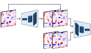
Figure 4. Simplified network schematics of (a) the baseline CNN, (b) cGAN-based PredictionNet and (c) ControlNet.
ControlNet uses a pre-trained PredictionNet that contains the dynamics of our data as a surrogate model to generate disturbance fields that change the evolution of the flow field in a direction suitable for a target, as follows:
 \begin{equation} {\rm Control}(X(t))=\Delta X, \quad {\rm Pred}(X(t)+\Delta X)=\tilde{Y}. \end{equation}
Here  $\Delta X$ represents the disturbance field added to the input field $X(t)$ and $\tilde {Y}$ is the disturbance-added prediction at time $t+T$. An important implication of ControlNet in this study is that it is a model-free method without restrictions, except for the strength of $\Delta X$. The objective function to be maximised includes the change in the vorticity field at a later time, as follows:
 \begin{equation} \mathop{\mathop{\mathrm{argmax}}}\limits_{w_c}\|{Y^*- \tilde{Y}}\|, \end{equation}
where  $w_c$ are the weight parameters of ControlNet. In the process of training of ControlNet, the weight parameters of ControlNet are updated in the direction maximising the change in the vorticity field at the target lead time. The already trained PredictionNet with fixed weight parameters is used in the prediction of controlled field as a surrogate model in training of ControlNet. Therefore, once the training of ControlNet is successful through maximisation of the loss based on the change in the vorticity field, the trained ControlNet can produce an optimum disturbance field. Whether the generated disturbance field is globally optimum, however, is not guaranteed. For the final form of the loss function, a spectral gradient loss term is additionally used to remove nonphysical noise (i.e. smoothing effect), and a CNN model is applied:
 \begin{align} L_{control}={-}\mathbb{E}_{X\sim p(X)} \left[\|{Y^*- \tilde{Y}}\|_2^2\right]+\theta L_{grad}, \quad L_{grad}=\mathbb{E}_{X\sim p(X)} \left[\|\boldsymbol{\nabla}_{\boldsymbol{x}}\left(\Delta X\right)\|_2^2\right], \end{align}
where  $\boldsymbol {\nabla }_{\boldsymbol {x}}$ denotes the gradient with respect to the coordinate directions. The coefficient $\theta$ controls the strength of smoothing effect, and it is adjusted depending on the order of data loss (see § 4.4). Figure 4(c) shows a simplified configuration of ControlNet.
3.2. Network architecture
A typical multiscale architecture of a CNN was used for both PredictionNet and ControlNet, as shown in figure 5(a). The architecture consists of six convolutional blocks, each composed of three convolutional layers with  $3 \times 3$ filter kernels (Conv. $3 \times 3$), called Convblk-m, named after their feature maps with different resolutions ( ${128/2^m}\times {128/2^m} \ (m=0,1,2,3,4,5)$). Here, the average pooled inputs $X^{(m)} (m=1,2,3,4)$ and the original input $X^{(0)}$ are concatenated to the feature map tensor at the beginning of each Convblk-m to be used as feature maps. One node point of a pooled input $X^{(m)}$ contains the compressed information of $2^m$ points of $X^{(0)}$. Using such an architecture enables all the spatial grid information of an input field, $X$, to be used to calculate a specific output point, even for the lowest-resolution feature maps. For example, the receptive field of Convblk-5 is $(2^5\times 7)\times (2^5\times 7)$, which means that all the spatial grid points of $X^{(0)}$ are used to calculate a point in the output. In addition, by sequentially using low- to high-resolution feature maps, the network can learn large-scale motion in the early stages, and then fill in the detailed features of small-scale characteristics in the deepest layers. As mentioned in § 2, the purpose of designing networks is to increase the prediction accuracy and determine the global optimum by considering the spectral properties of the flow. However, depending on the flow features or characteristics of the flow variables, we can expect that accurate results can be obtained even using only a small input domain with a size similar to $L$ for cost-effectiveness. Furthermore, periodic padding was used to maintain the size of the feature maps after convolutional operations, because the biperiodic boundary condition was applied spatially. The feature maps generated from Convblk-(m+1) must be extended through upscaling to be concatenated and used with the following pooled input $X^{(m)}$ (i.e. doubling the size via upsampling). In this process, a transposed convolution is used to minimise the non-physical phenomena. After upscaling, $X^{(m)}$ is concatenated to the feature map tensor and then Convblk-m operations are performed. Finally, after the original input field $X^{(0)}$ is concatenated, the operations of Convblk-0 are performed, and the output of resolution ${128}\times {128}$ is generated depending on the network, prediction result $\textrm {Pred}(X)=Y^*$, or disturbance field $\textrm {Control}(X)=\Delta X$. Detailed information on the architectures of PredictionNet and ControlNet, including the number of feature maps used in each Convblk, are presented in table 1. A leaky rectified linear unit (LReLU) is used as an activation function to add nonlinearities after each convolutional layer. This was not applied to the last layer of Convblk-0, to prevent nonlinearity in the final output.

Figure 5. Network architecture of (a) PredictionNet (the generator of cGAN) and ControlNet and (b) discriminator of cGAN.
Table 1. Number of feature maps used at each convolutional layer of Convblks and Disblks.

The discriminator of PredictionNet to which cGAN is applied has a symmetric architecture for the generator (PredictionNet), as shown in figure 5(b). Here  $X^{0}$ is concatenated with the target or the prediction result for the input of the discriminator as a condition. In contrast to the generator, convolutional operations are performed from high to low resolutions, named with each convolutional block as Disblk-m. Average pooling was used for downsampling to half the size of the feature maps. After the operation of Disblk-5, its output feature maps passed through two fully connected layers (with output dimensions of $1\times 1\times 256$ and $1\times 1\times 1$) to return a scalar value. The numbers of feature maps used for each Disblk are presented in table 1. The baseline CNN model takes the same architecture as PredictionNet but is trained without adversarial training through the discriminator.
4. Results
4.1. PredictionNet: prediction of the vorticity field at a finite lead time
In this section, we discuss the performance of PredictionNet in predicting the target vorticity field at  $t+T$ using the field at $t$ as the input. The considered lead times $T$ are $0.25T_L, 0.5T_L, T_L$ and $2T_L$ based on the observation that the autocorrelation of the vorticity at each lead time dropped to 0.71, 0.49, 0.26 and 0.10, respectively (figure 2a). The convergence behaviour of the L2 norm-based data loss of the baseline CNN and cGAN models for various lead times in the process of training is shown for 100 000 iterations with a batch size of 32 in figure 6. It took around 2 and 5.4 h for CNN and cGAN, respectively, on a GPU machine of NVIDIA GeForce RTX 3090. Although the baseline CNN and PredictionNet have the exact same architecture (around 520 000 trainable parameters based on table 1), cGAN includes a discriminator to be trained comparable to the generator with many complex loss terms; thus, the training time is almost tripled. Both models yielded good convergence for lead times of up to $0.5T_L$, whereas overfitting was observed for $T=T_L$ and $2T_L$ in both models. Since the flow field is hardly correlated with the input field [correlation coefficient (CC) of 0.26 and 0.10], it is naturally more challenging to train the model that can reduce a mean-squared error (MSE)-based data loss, a pointwise metric that is independent of the spatial distribution. One notable observation in figure 6 is that for lead times beyond $T_L$, CNN appears to exhibit better performance than cGAN, as evidenced by its smaller converged data loss. However, as discussed later, the pointwise accuracy alone cannot encompass all the aspects of turbulence prediction due to its various statistical properties. In addition, although the only loss term of CNN is the pointwise MSE except the weight regularisation, the magnitude of its converged data loss also remains significant.

Figure 6. Convergence of data loss depending on the lead time of (a) baseline CNN and (b) cGAN. The order of the converged value increases as the lead time increases. In addition, relatively large overfitting was observed in the case of  $T=2T_L$.
As an example of the test of the trained network, for unseen input data, the fields predicted by cGAN and CNN were compared against the target data for various lead times, as shown in figure 7. In the test of cGAN, only PredictionNet was used to generate or predict flow field at the target lead time. Hereinafter, when presenting performance results for the instantaneous field, including figure 7 and all subsequent statistics, we only brought the results for input at  $t_0$. This choice was made because the difficulty of tasks that the models have to learn is much larger at earlier time since flow contains more small-scale structures than later times due to decaying nature. Therefore, performance test for input data at $t_0$ is sufficient for test of the trained network. For short lead-time predictions, such as $0.25T_L$, both cGAN and CNN showed good performance. However, for a lead time of $0.5T_L$, the prediction by the CNN started displaying a blurry image, whereas cGAN's prediction maintained small-scale features relatively better than CNN. This blurry nature of the CNN worsened the predictions of $T_L$ and $2T_L$. Although cGAN's prediction also deteriorated as the lead time increased, the overall performance of cGAN, particularly in capturing small-scale variations in the field, was much better than that of the CNN even for $T_L$ and $2T_L$.

Figure 7. Visualised examples of the performance of the cGAN and CNN for one test dataset. (a) Input field at  $t_0$, prediction results at the lead time (b) $0.25T_L$, (c) $0.5 T_L$, (d) $T_L$ and (e) $2T_L$. Panels (b i,c i,d i,e i), (b ii,c ii,d ii,e ii) and (b iii,c iii,d iii,e iii) show the target DNS, cGAN predictions and CNN predictions, respectively.
A quantitative comparison of the performances of the cGAN and CNN against the target in the prediction of various statistics is presented in table 2. The CC between the prediction and target fields or, equivalently, the MSE by the cGAN shows a better performance than that by the CNN for lead times of up to  $0.5T_L$, even though both the cGAN and CNN predicted the target field well. For $T_L$, the CC by cGAN and CNN was 0.829 and 0.868, respectively, indicating that the predictions by both models were not poor, whereas the predictions by both models were quite poor for $2T_L$. Once again, for lead times larger than $T_L$, CNN shows better performance on the pointwise metrics according to the trend of data loss. Conversely, the statistics related to the distribution of vorticity, such as the r.m.s. value or standardised moments ( $\hat {\mu }_n=\mu _n/\sigma ^n$, where $\mu _n=\langle (X-\langle X\rangle )^n\rangle$ is the $n$th central moments and $\sigma =\sqrt {\mu _2}$ is the standard deviation), clearly confirm that the cGAN outperforms the CNN for all lead times, and the prediction by the cGAN was much closer to the target than that of the CNN, even for $T_L$ and $2T_L$. Furthermore, the prediction of the Kolmogorov length scale ( $\eta =(\nu ^3/\varepsilon )^{1/4}$) and dissipation ( $\varepsilon =2\nu \langle S_{ij}S_{ij}\rangle$, $\varepsilon '=\varepsilon t^{*3}/\lambda ^{*2}$, where $S_{ij}$ is the strain rate tensor) by cGAN was more accurate than that by the CNN, as presented in table 2. All these qualitative and quantitative comparisons clearly suggest that the adversarial learning of the cGAN tends to capture the characteristics of turbulence data better than the CNN, which minimises the pointwise MSE only. The superiority of the cGAN is more pronounced for large lead times, for which small-scale turbulence features are difficult to predict.
Table 2. Quantitative comparison of the performance of the cGAN and CNN against the target in the prediction of the CC, MSE and r.m.s., and the  $n$th standardised moments, Kolmogorov length scale ( $\eta$) and dissipation rate ( $\varepsilon '$) depending on the lead time for the input at $t_0$. All the dimensional data such as MSE, r.m.s. and $\varepsilon '$ are provided just for the relative comparison.

Detailed distributions of probability density functions (p.d.f.s) of vorticity, two-point correlation functions and enstrophy spectra ( $\varOmega (k)={\rm \pi} k\varSigma _{|\boldsymbol {k}|=k}|\hat {\omega }(\boldsymbol {k})|^2$ where $\hat {\omega }(\boldsymbol {k},t)=\mathcal {F}\{\omega (\boldsymbol {x},t)\}$) of the target and prediction fields by the cGAN and CNN are compared for all lead times in figure 8. Both the cGAN and CNN effectively predicted the target p.d.f. distribution for lead times of up to $T_L$, whereas the tail part of the p.d.f. for $2T_L$ was not effectively captured by the cGAN and CNN. The difference in performance between the cGAN and CNN is more striking in the prediction of $R_{\omega }(r)$ and $\varOmega (k)$. The values of $R_{\omega }(r)$ and $\varOmega (k)$ obtained by the cGAN almost perfectly match those of the target for all lead times, whereas those predicted by the CNN show large deviations from those of the target distribution progressively with the lead time. In the prediction of the correlation function, the CNN tends to produce a relatively slow decaying distribution compared with the cGAN and the target, resulting in a much larger integral length scale for all lead times. In particular, it is noticeable that even for a short lead time of $0.25T_L$, the CNN significantly underpredicts $\varOmega (k)$ in the high-wavenumber range, and this poor predictability propagates toward the small-wavenumber range as the lead time increases, whereas cGAN produces excellent predictions over all scale ranges, even for $2T_L$. This evidence supports the idea that adversarial learning accurately captures the small-scale statistical features of turbulence.

Figure 8. Comparison of statistics such as the p.d.f., two-point correlation and enstrophy spectrum of the target and prediction results at different lead times (a)  $0.25T_L$, (b) $0.5 T_L$, (c) $T_L$ and (d) $2T_L$ for the same input time point $t_0$.
To quantify in more detail the differences in the prediction results by cGAN and CNN models, scale decomposition was performed by decomposing the fields in the wavenumber components into three regimes: large-, intermediate- and small-scale fields, as in the investigation of the temporal correlation in figure 2(b). The decomposed fields predicted for the lead time of  $T_L$ by the cGAN and CNN, for example, were compared with those of the target field, as shown in figure 9. As shown in figure 2(b), the large-scale field $(k\leq 4)$ persists longer than the total fields with an integral time scale 1.4 times larger than that of the total field, whereas the intermediate-scale field $(4< k\leq 20)$ and the small-scale field $(20< k)$ decorrelate more quickly than the total field with integral time scales one-fourth and one-twelfth of that of the total field, respectively. Given that the intermediate- and small-scale fields of the target field are almost completely decorrelated from the initial field at a lead time of $T_L$ as shown in figure 2(b), the predictions of those fields by the cGAN shown in figure 9(c,d) are excellent. The cGAN generator generates a small-scale field that not only mimics the statistical characteristics of the target turbulence but is also consistent with the large-scale motion of turbulence through adversarial learning. A comparison of the decomposed fields predicted by the cGAN and CNN for other lead times is presented in Appendix B. For small lead times, such as $0.25T_L$ and $0.5T_L$, the cGAN predicted the small-scale fields accurately, whereas those produced by the CNN contained non-negligible errors. For $2T_L$, it is difficult to predict using both models even with the large-scale field. On the other hand, the CC of decomposed fields between the target and predictions, provided in table 4 (Appendix B), did not demonstrate the superiority of the cGAN over the CNN. This is attributed to the fact that pointwise errors such as the MSE or CC are predominantly determined by the behaviour of large-scale motions. The pointwise MSE is the only error used in the loss function of the CNN, whereas the discriminator loss based on the latent variable is used in the loss function of the cGAN in addition to the MSE. This indicates that the latent variable plays an important role in predicting turbulent fields with multiscale characteristics.

Figure 9. Prediction results of the scale-decomposed field for lead time  $T_L$: (a) original fields, (b) large scales ( $k\leq 4$), (c) intermediate scales ( $4< k \leq 20$) and (d) small scales ( $k>20$). Panels (a i,b i,c i,d i), (a ii,b ii,c ii,d ii) and (a iii,b iii,c iii,d iii) display the target DNS fields, cGAN predictions and CNN predictions, respectively.
Table 4. Correlation coefficient between the target and prediction of the scale-decomposed fields depending on the lead time.

In the prediction of the enstrophy spectrum, the cGAN showed excellent performance, compared with the CNN, by accurately reproducing the decaying behaviour of the spectrum in the small-scale range, as shown in figure 8. The average phase error between the target and predictions by the cGAN and CNN is shown in figure 10. For all lead times, the phase error of the small-scale motion approaches  ${\rm \pi} /2$, which is the value for a random distribution. For short lead times $0.25T_L$ and $0.5T_L$, the cGAN clearly suppressed the phase error in the small-scale range compared with the CNN, whereas for $T_L$ and $2T_L$, both the cGAN and CNN poorly predicted the phase of the intermediate- and small-scale motions, even though the cGAN outperformed the CNN in predicting the spectrum.

Figure 10. Prediction results of the phase error of each model depending on  $T$.
$T$.
The performance of PredictionNet in the prediction of velocity fields is presented in Appendix C, where several statistics, including the p.d.f. of velocity, two-point correlation and p.d.f. of the velocity gradient are accurately predicted for all lead times. The superiority of the cGAN over the CNN was also confirmed.
4.2. Role of the discriminator in turbulence prediction
In the previous section, we demonstrated that adversarial learning using a discriminator network effectively captured the small-scale behaviour of turbulence, even when the small-scale field at a large lead time was hardly correlated with that of the initial field. In this section, we investigate the role of the discriminator in predicting turbulence through the behaviour of the latent variable, which is the output of the discriminator. Although several attempts have been made to disclose the manner in which adversarial training affects the performance of the generator and the meaning of the discriminator output (Creswell et al. Reference Creswell, White, Dumoulin, Arulkumaran, Sengupta and Bharath2018; Yuan et al. Reference Yuan, He, Zhu and Li2019; Goodfellow et al. Reference Goodfellow, Pouget-Abadie, Mirza, Xu, Warde-Farley, Ozair, Courville and Bengio2020), there have been no attempts to reveal the implicit role of the latent variable in recovering the statistical nature of turbulence in the process of a prediction.
In the current cGAN framework, the discriminator network is trained to maximise the difference between the expected value of the latent variable of the target field  $D(Y,X)$ and that of the prediction $D(Y^*,X)$, whereas the generator network is trained to maximise $D(Y^*,X)$ and to minimise the pointwise MSE between $Y$ and $Y^*$. Therefore, through the adversarial learning process, the discriminator is optimised to distinguish $Y^*$ from $Y$, whereas the generator evolves to produce $Y^*$ by reflecting on the optimised latent variable of the discriminator and minimising the MSE between $Y$ and $Y^*$. The input field $X$ is used as a condition in the construction of the optimal latent variable in the discriminator network. The behaviour of the expected value of the latent variable of the target and generated fields ( $L_{true}$ and $L_{false}$) and their difference ( $L_{true}-L_{false}$) as learning proceeds for all lead times are illustrated in figure 11. Because of the regularisation of the latent variable by $L_{drift}(=L_{true}^2)$ in the loss function of the discriminator, both $L_{true}$ and $L_{false}$ remain around zero, although they sometimes oscillate significantly. As the learning proceeds, $L_{true}-L_{false}$ quickly decays initially owing to the suppression of the MSE and continues to decrease to zero for $0.25T_L$ and $0.5T_L$ but to a finite value for $T_L$ and $2T_L$. The intermittent transition of $L_{true}-L_{false}$ between a finite value and zero for $0.25T_L$ and $0.5T_L$ clearly suggests that the generator and discriminator operate competitively in an adversarial manner. As the generator improves, the difference monotonically decreases and occasionally exhibits sudden suppression. When sudden suppression occurs, the discriminator evolves to distinguish $Y^*$ from $Y$ by finding a better criterion latent variable, resulting in a sudden increase in the difference. Ultimately, when the generator can produce $Y^*$ that is indistinguishable from $Y$ by any criterion proposed by the discriminator, the difference converges to zero, as shown in the cases of $0.25T_L$ and $0.5T_L$. However, for $T_L$ and $2T_L$, such an event never occurs; $L_{true}-L_{false}$ monotonically decreases and tends toward a finite value, implying that the discriminator wins and can distinguish $Y^*$ from $Y$. Although the generator cannot produce $Y^*$ to beat the discriminator, $Y^*$ retains the best possible prediction.

Figure 11. Evolution over training iteration of (a)  $L_{true}$ and $L_{false}$ and (b) their difference evaluated every 2000 iterations.
To understand the mechanism in more detail that the discriminator uses to distinguish a generated field from a target field, the behaviour of the distribution of the latent variable during the learning process was investigated, because the latent variable plays a key role in the discriminator network. The distribution of the discriminator output of the generated field  $D(Y^*,X)$ at four iterations during the learning process is marked with a green circle in figure 11(b) for all lead times and is compared with that of the target field $D(Y,X)$ in figure 12. The distributions of latent variable of the scale-decomposed target field $D(Y^S,X)$, $D(Y^I,X)$ and $D(Y^L,X)$ are also compared for analysis, where $Y^S, Y^I$ and $Y^L$ are scale-decomposed from $Y$ in the same manner, as shown in figure 2. Here, an additional 500 fields, in addition to the 50 test fields, were used to extract a smooth distribution of the latent variables of the target field and scale-decomposed target fields. For easy comparison, the mean value of the latent variable for the target field was shifted to zero.

Figure 12. Distributions of discriminator output (latent variable) for various fields at several iterations: (a)  $T=0.25T_L$, (b) $T=0.5T_L$, (c) $T=T_L$ and (d) $T=2T_L$. All distributions are shifted by the target mean to fix the target distribution at the zero mean. The vertical black solid line indicates the target mean (zero) and the red line is the prediction mean. When the mean difference between the target and prediction is smaller than 0.5, the vertical lines are omitted for visibility.
For all lead times, as learning proceeded, the distributions of  $D(Y,X)$ and $D(Y^*,X)$ became narrower, with the mean values of $D(Y,X)$ and $D(Y^*,X)$ becoming closer to each other (the gap between the two vertical lines decreases). This indicates that, as the generator improves in producing $Y^*$ closer to $Y$, the discriminator becomes more efficient in distinguishing $Y^*$ from $Y$ because only the mean values are compared in the discrimination process and the narrower distributions yield the sharper mean values. Even when the mean values of $D(Y,X)$ and $D(Y^*,X)$ are almost the same (18 000 and 124 000 iterations for $0.25T_L$ and 84 000 and 190 000 iterations for $0.5T_L$; see figure 12a,b), a more optimal discriminator at later iterations yields a narrower distribution. The collapse of the distribution of $D(Y,X)$ and $D(Y^*,X)$ in the second column for $0.25T_L$ and $0.5T_L$ occurs when the discriminator falls into a local optimum during training, implying that the predicted and target fields are indistinguishable by the discrimination criterion right at that iteration. However, as the criterion is jittered in the next iterations, the two fields become distinct again as shown in the third column. Eventually, when the two fields become indistinguishable by any criterion after sufficient iterations, almost perfect collapse of very narrow distributions is achieved as shown in the fourth column for $0.25T_L$ (the collapse shown in the fourth column for $0.5T_L$ occurs in another local optimum). For $T_L$ and $2T_L$, for which perfect training of the discriminator was not achieved, however, distributions of $D(Y,X)$ and $D(Y^*,X)$ hardly change with iteration although the mean values are getting closer to each other very slowly.
In the comparison with the scale-decomposed target field, we observe that for  $0.25T_L$ and $0.5T_L$, the distribution of the latent variable of the small-scale target field among all the scale-decomposed target fields is closest to that of the target field and generated field, whereas that of the intermediate-scale target field is closest to that of the target and generated fields for $T_L$ and $2T_L$. This suggests that a small-scale (or intermediate) field in the target field plays the most critical role in discriminating the generated field from the target field for $0.25T_L$ and $0.5T_L$ (or $T_L$ and $2T_L$). If the generator successfully produces $Y^*$ similar to $Y$ for $0.25T_L$ and $0.5T_L$, and the predictions for $T_L$ and $2T_L$ are incomplete, the small-scale fields for $T_L$ and $2T_L$ are useless for discriminating the generated field from the target field, and the intermediate-scale field is partially useful. Considering the possible distribution of the functional form of the latent variable may provide a clue to this conjecture. The latent variable, which is the output of the discriminator network shown in figure 5(b), and a function of the input fields $Y$ (or $Y^*$) and $X$, can be written as
 \begin{align} D(Y,X) = \sum_{k_x, k_y} \hat{D}^Y(k_x \Delta x, k_y \Delta y; w_d, \epsilon_L) \hat{Y}(k_x,k_y) +\sum_{k_x, k_y} \hat{D}^X(k_x \Delta x, k_y \Delta y; w_d, \epsilon_L) \hat{X}(k_x,k_y), \end{align}
where  $\hat {Y}$ and $\hat {X}$ are the Fourier coefficients of $Y$ and $X$, respectively. Here $\Delta x$, $\Delta y$, $w_d$ and $\epsilon _L$ are the grid sizes in each direction, weights of the discriminator network and slope of the LReLU function for the negative input, respectively. This linear relationship between the input and output is a consequence of the linear structure of the discriminator network: the convolution, average pooling, and full connection operations are linear, and the LReLU function is a piecewise linear function such that either one or $\epsilon _L$ is multiplied by the function argument, depending on its sign. Although $\hat {D}^Y$ is an undetermined function, a possible shape can be conjectured. For $0.25T_L$ and $0.5T_L$, $\hat {D}^Y$ of the optimised discriminator network has more weight in the small-scale range than in other scale ranges such that the latent variable is more sensitive to the small-scale field; thus, it better discriminates the generated field from the target field. Similarly, for $T_L$ and $2T_L$, $\hat {D}^Y$ has more weight in the intermediate-scale range than in the other ranges, and discrimination is limited to the intermediate-scale field because the small-scale field is fully decorrelated; thus, it is no longer useful for discrimination. Although the manner in which $\hat {D}^X$ conditionally influences learning is unclear, the scale-dependent correlation of the target field with the initial input field appears to be captured by $\hat {D}^X$. More importantly, it is conjectured that through $\hat {D}^X$, the large-scale motions of the input field play an important role in determining the small-scale motions of the generated field at finite lead times since the enstrophy cascades towards the small scales in 2-D turbulence. This scale-selective and scale-interaction feature of the discriminator appears to be the key element behind the successful prediction of the small-scale characteristics of turbulence at finite lead times. Here, the generator implicitly learns system characteristics embedded in data to deceive the discriminator with such features; thus, it is extremely challenging to provide an exact mechanism for how prediction performance is comprehensively enhanced, particularly in terms of physical and statistical attributes through adversarial training. However, we clearly showed that such a successful prediction of turbulence, even down to small scales, is possible through adversarial learning and not by the use of a CNN, which enforces suppression of the pointwise MSE only.
One last question that may arise in this regard is whether introducing physical constraints explicitly into the model, rather than using implicit competition with an additional network, could also be effective. To explore this, we incorporated the enstrophy spectrum as an explicit loss term into the objective function of the CNN model to address the performance issues associated with small-scale features. As shown in the relevant results presented in Appendix D, adding the enstrophy loss alone did not lead to better performance although the enstrophy spectrum was better predicted. This confirms that the adoption of an implicit loss based on the latent variable in cGAN is effective in reflecting the statistical nature of turbulence, particularly the small-scale characteristics and the interactions between different scales. Once again, it is stressed that recovering the statistical nature of the small-scale motions along with learning the scale interaction through the enstrophy cascade between the large-scale and small-scale motions can accurately predict turbulence in all scales even at finite lead times and that cGAN-based algorithm possesses such capability.
4.3. PredictionNet: single vs recursive prediction
In the previous section, we observed that the prediction performance for large lead times deteriorated naturally because of the poor correlation between the target field and the initial input field. An improved prediction for large lead times may be possible if recursive applications of the prediction model for short lead times are performed. Conversely, recursive applications may result in the accumulation of prediction errors. Therefore, there is an optimal model that can produce the best predictions. In this regard, since the performance of CNN models itself falls short of PredictionNet across all lead times, a more significant error accumulation is expected to arise. Thus, we would focus on analysing the recursive prediction results using PredictionNet. Nevertheless, we also presented the results of CNN models, not only to highlight the improvements through recursive prediction for large lead-time prediction but also to compare how much further enhancement is achieved when utilising PredictionNet. A similar concept was tested for weather prediction (Daoud, Kahl & Ghorai Reference Daoud, Kahl and Ghorai2003).
For example, for the prediction of a large lead time  $2T_L$, four base models trained to predict the lead times $0.125T_L$, $0.25T_L$, $0.5T_L$ and $T_L$ were recursively applied 16, 8, 4 and 2 times, respectively, and compared against the single prediction as shown in figure 13. All recursive applications produced better predictions than the corresponding single prediction, and among them, four recursive applications of the cGAN model for $0.5T_L$ yielded the best results. Eight recursive applications of CNN model for $0.25T_L$, however, produces the best prediction. For all lead times, the best prediction was sought; the performances of all recursive predictions by cGAN and CNN are compared in table 3 in terms of performance indices, such as the CC and MSE and statistical quantities, including r.m.s., $\hat {\mu }_4$ and dissipation rate. Here, we observed that the performance difference depending on the input time point varies significantly depending on the base model; thus, the time-averaged values for CC and MSE from $t_0$ to $t_{100}$ as input are presented to ensure fair comparison, unlike § 4.1. The CC and MSE values are plotted in figure 14. As expected, there exists an optimum base model producing the best performance for each lead time. Recursive prediction was more effective for large lead times ( $T_L$ and $2T_L$) than for short lead times ( $0.25T_L$ and $0.5T_L$) for cGAN model. For $2T_L$, the CC improved from 0.4530 to 0.7394 and MSE decreased from 0.506 to 0.250 through the best recursive applications of cGAN model. The predicted statistics exhibited a consistent improvement. For $T_L$, the recursive applications show similar improvements. However, for $0.25T_L$ and $0.5T_L$, even though the recursive applications produced slightly better performance in terms of the CC and MSE, the statistics predicted by the single prediction are more accurate than those of the recursive prediction. However, recursive applications of CNN model do not show a monotonic behaviour in CC or MSE; for $T_L$, eight applications of CNN model trained for $0.125T_L$ yield the best prediction, whereas two applications of CNN model for $T_L$ produces the best prediction for $2T_L$. Finally, the prediction of the enstrophy spectrum by recursive prediction also yielded an improvement over the single prediction, as shown in figure 15. In particular, it is noticeable that eight recursive applications of CNN model trained for $0.25T_L$ yielded relatively better spectrum than the single prediction. However, the performance of prediction was not good enough as shown in figure 13(c).

Figure 13. Visualised prediction results for  $T=2T_L$ of (a) target DNS field and single predictions using cGAN and CNN, (b) cGAN recursive predictions and (c) CNN recursive predictions.

Figure 14. Plots of the CC and MSE of the recursive predictions in terms of the lead time of the base recursive model. Only  $T_L$ and $2T_L$ cases are included for CNN for visibility.

Figure 15. Enstrophy spectra of the best case of recursive prediction compared with the target and single prediction for  $T=2T_L$ using (a) cGAN and (b) CNN.
It is noteworthy that for the prediction at  $T_L$ and $2T_L$, the best recursive prediction is made using two and four consecutive applications of the model trained for $0.5T_L$, respectively, whereas for the prediction at $0.5T_L$, any recursive prediction does not improve the performance significantly. This indicates that the prediction model for the lead time up to $0.5T_L$ is almost ‘complete’ in that the small-scale motions at up to $0.5T_L$ can be entirely recovered from the input data. A plausible interpretation of this observation is that the time required for the enstrophy to cascade to the smallest scale in the current 2-D turbulence is within $0.5T_L$. Therefore, the prediction at $T_L$ or $2T_L$ is inevitably incomplete.
Table 3. Statistical results of recursive predictions for various values of  $T$ including the single prediction at the last entries. Best prediction for each lead time by cGAN is bold-faced.

4.4. ControlNet: maximisation of the propagation of the control effect
In this section, we present an example of flow control that uses the high-accuracy prediction model developed in the previous section as a surrogate model. By taking advantage of the prediction capability of the model, we can determine the optimum control input that can yield the maximum modification of the flow in the specified direction with a fixed control input strength. In particular, we trained ControlNet to find a disturbance field that produces the maximum modification in the vorticity field over a finite time period with the constraint of a fixed r.m.s. of the disturbance field. Similar attempts to control 2-D decaying turbulence were made by Jiménez (Reference Jiménez2018) and Yeh et al. (Reference Yeh, Meena and Taira2021). Jiménez (Reference Jiménez2018) modified a part of a vorticity field to identify dynamically significant sub-volumes in 2-D decaying turbulence. The influence on the future evolution of the flow was defined as significance using the L2 norm of the velocity field. Then, the significance of the properly labelled regions was compared by turning the vorticity of specific regions on and off. They showed that vortices or vortex filaments are dynamically significant structures, and interstitial strain-dominated regions are less significant. In contrast, Yeh et al. (Reference Yeh, Meena and Taira2021) developed a method called network-broadcast analysis based on network theory by applying Katz centrality (Katz Reference Katz1953) to identify key dynamical paths along which perturbations amplify over time in 2-D decaying turbulence. Two networks (composed of nodes and edges, not neural networks), the Biot–Savart (BS) network and Navier–Stokes (NS) network, with different adjacency matrices were investigated. In the former case, vortex structures similar to those in Jiménez (Reference Jiménez2018), and in the latter case, opposite-sign vortex pairs (vortex dipoles) were the most effective structures for perturbation propagation. However, both studies confined the control disturbance field either by localising the modification for control by dividing the domain into cell units (Jiménez Reference Jiménez2018), or by considering the perturbation using the leading singular vector of an adjacency matrix calculated from a pulse in a predefined shape (Yeh et al. Reference Yeh, Meena and Taira2021). However, the disturbance field considered in ControlNet is free of shape, and the only constraint is the strength of the disturbance field in terms of the fixed r.m.s. of the input field.
As a surrogate model for the time evolution of the disturbance-added initial field, PredictionNet trained for a lead time of  $0.5T_L$ was selected for the control test. ControlNet is trained to generate an optimum disturbance field $\Delta X$ that maximises the difference between the disturbance-added prediction $\tilde {Y} (=\textrm {Pred}(X+\Delta X))$ and the original (undisturbed) prediction $Y^*$. If the strength of $\Delta X$ is too large, causing $X+\Delta X$ to deviate from the range of dynamics of the pre-trained PredictionNet, the surrogate model will not function properly, resulting in $\tilde {Y}$ being different from the ground-truth solution $\mathscr{N}(X+\Delta X)$. Here, $\mathscr{N}()$ is the result of the Navier–Stokes simulation, with the input as the initial condition. Here $\tilde {Y}$, using disturbances with various strengths of the r.m.s. of the input field ( $\Delta X_{rms}=0.1, 0.5, 1, 5, 10, 20\,\%$ of $X_{rms}$), were compared with the corresponding $\mathscr {N}(X+\Delta X)$. We confirmed that PredictionNet functions properly within the tested range (Appendix E). Therefore, the effect of the disturbance strength was not considered; thus, we only present the 10 % case. Coefficient $\theta$ related to the smoothing effect was fixed at 0.5 for $\Delta X_{rms}=0.1X_{rms}$ through parameter calibration. Figure 16 shows the data loss trend of ControlNet for $\Delta X_{rms}=0.1X_{rms}$, which is maximised as the training progresses, confirming successful training.

Figure 16. Convergence of the data loss of ControlNet for  $0.5T_L$. Here $\Delta X_{rms}=0.1X_{rms}$.
Figure 17 presents a visualisation of the effect of the control input on one of the test data. Figure 17(a) shows the input vorticity field and corresponding prediction at  $T=0.5T_L$. Figure 17(b) shows the disturbance field generated by ControlNet $\Delta X_C$, disturbance-added prediction, and difference between the undisturbed and disturbance-added predictions, demonstrating that the control effect is effectively propagated and amplified at $T=0.5T_L$. The MSE between $\tilde {Y}_{C}$ and $Y^*$ is 0.757, indicating a substantial change. A prominent feature of $\Delta X_{C}$ is its large-scale structure. To verify whether the propagation of the control effect of $\tilde {Y}_C$ was maximised under the given conditions, we considered three additional disturbance fields. Inspired by the results of Jiménez (Reference Jiménez2018) and the claim of Yeh et al. (Reference Yeh, Meena and Taira2021) regarding their BS network, in which vortices have the greatest effect on the future evolution of the base flow, we considered a 10 % scaled input disturbance $\Delta X_{SI}\ (=0.1 X)$. Another disturbance field due to a single Taylor vortex $\Delta X_{TV}$ extracted from the NS network of Yeh et al. (Reference Yeh, Meena and Taira2021), which is best for amplifying the control effect when applied to a vortex dipole rather than the main vortex structures, is considered in the following form:
 \begin{equation} \Delta X_{TV}(x,y)=\epsilon\delta(x_c,y_c)= \epsilon(2/r_{\delta}-r^2/r^3_{\delta})\exp[{-}r^2/(2r^2_{\delta})], \end{equation}
where  $r=\sqrt {(x-x_c)^2+(y-y_c)^2}$ with vortex centre $(x_c,y_c)$. Here $\epsilon$ represents the amplitude of the Taylor vortex, and it is adjusted to maintain the r.m.s. of the disturbance at 0.1 $X_{rms}$. We set $r_{\delta }$ to $r_{\delta }={\rm \pi} /k_{max}$, where $k_{max}=4$ denotes the wavenumber with the maximum value in the enstrophy spectra. Finally, the disturbance field in the form of a Taylor–Green vortex $\Delta X_{TG}$ approximating the disturbance field of ControlNet is considered as follows:
 \begin{equation} \Delta X_{TG}(x,y)=\epsilon \sin \left(\frac{1}{\sqrt{2}}(x-x_c-y+y_c)\right) \sin \left(\frac{1}{\sqrt{2}}(x-x_c+y-y_c)\right), \end{equation}
indicating the largest vortex in the  $[0,2{\rm \pi} )^2$-domain. For $\Delta X_{TV}$ and $\Delta X_{TG}$, the optimum location of $(x_c,y_c)$ that yielded the greatest propagation was determined through tests using PredictionNet.

Figure 17. Visualised example of disturbance fields: (a) input and the undisturbed prediction, (b) the optimum disturbance ( $\textrm {Control}(X)$), disturbance-added prediction ( $\textrm {Pred}(X+\Delta X_C)$) and the difference. Comparison cases of (c) $\Delta X_{SI}$, (d) $\Delta X_{TV}$ and (e) $\Delta X_{TG}$.
The disturbance-added predictions  $\tilde {Y}_{SI}$ and $\tilde {Y}_{TV}$ and their differences from the undisturbed prediction $Y^*$ using $\Delta X_{SI}$ and $\Delta X_{TV}$ located at the optimum position as disturbances, respectively, are shown in figure 17(c,d). The difference fields show that these disturbances do not significantly change the field. MSE values for $\tilde {Y}_{SI}$ and $\tilde {Y}_{TV}$ against the undisturbed prediction are 0.039 and 0.402, respectively, which are much smaller than the corresponding value of 0.757 for $\tilde {Y}_{C}$, as shown in figure 18(a). From this comparison, it can be conjectured that because the goal of control is to maximise the pointwise MSE of the vorticity against the undisturbed prediction, the large-scale disturbance of the vorticity is more effective in displacing and deforming the vorticity field. The enstrophy spectra of the disturbance fields shown in figure 18(b) confirm that $\Delta X_C$ has a peak value at $k=1$, representing the largest permissible scale in the given domain, whereas $\Delta X_{TV}$ and $\Delta X_{SI}$ have peak values at $k=2$ and $k=4$, respectively, under the constraint that the r.m.s. value of all disturbances is $0.1X_{rms}$. This observation leads to the consideration of the largest Taylor–Green vortex-type disturbance $\Delta X_{TG}$ in the domain given by (4.3). The distribution of the optimum location of $\Delta X_{TG}$ shown in figure 17(e), yielding the greatest propagation coincides with that of $\Delta X_C$ shown in figure 17(b) (except for the sign owing to the symmetry in the propagation effect, as shown in the third panel of figure 17b,e). The MSE of $\tilde {Y}_{TG}$ against $Y^*$ was 0.726, which was slightly smaller than 0.757 of $\tilde {Y}_C$ (figure 18a). All these comparisons suggest that the largest-scale disturbance is the most effective in modifying the vorticity field through displacement or distortion of the given vorticity field. To verify whether the location of the largest-scale disturbance $\Delta X_C$ was indeed globally optimal, tests were conducted with a phase-shifted $\Delta X_C$. We consider two types of phase shifting for the wavenumber components $\hat {\Delta X}_C \exp (\textrm {i} k_x l_x + \textrm {i} k_y l_y)$: one with randomly selected $l_x$ and $l_y$ uniformly applied to all wavenumbers and the other with randomly selected phases differently applied to each wavenumber. The test results confirm that the maximum MSE was obtained for $\Delta X_C$ (without a phase shift), with the minimum MSE found at 0.2 among the 1000 trial disturbances considered with randomly selected phases, as shown in figure 18(a). Here $\Delta X_{TG,min}$ corresponds to one of the $\Delta X_{TG}$ tests yielding the minimum modification with an MSE of approximately 0.45. The wide range of MSE for the largest-scale disturbance indicates that the location of the largest-scale disturbance is important for modifying the flow field.

Figure 18. (a) Comparison of MSEs between various  $\tilde {Y}$ and $Y^*$ using different disturbance fields. Black dots denote the sorted MSE of phase-shifted $\Delta X_C$. The first node of black dots (red dashed line) shows the result of the optimum $\Delta X_{C}$. (b) Enstrophy spectra of the input $X$,
$X$,  $\Delta X_{C}$, $\Delta X_{SI}$ and $\Delta X_{TV}$.
To confirm the optimality of  $\Delta X_C$ in real flow, full Navier–Stokes simulations were performed further than $0.5T_L$ using the disturbance-added initial conditions for $\Delta X_{C}$, $\Delta X_{SI}$, $\Delta X_{TV}$ and $\Delta X_{TG}$. The visualisation results of the propagation over the time horizon are shown in figure 19, and the behaviour of the normalised RMSE over time is shown in figure 19(e). Therefore, the propagation by large-scale disturbances such as $\Delta X_{C}$ and $\Delta X_{TG}$ is much more effective than that by $\Delta X_{SI}$ and $\Delta X_{TV}$ even up to longer than $T_L$. Moreover, the surrogate model functions properly for $\Delta X_{rms}=0.1X_{rms}$ based on the comparison between the results at $0.5T_L$ in figure 19 and those in the third column (difference fields) in figure 17 for each disturbance. The RMSE of $\Delta X_C$ and $\Delta X_{TG}$ behave almost indistinguishably as shown in figure 19(e) for all test periods.

Figure 19. Simulated propagations of the control effect along with the time horizon presented by differences between the disturbance-added simulations and the original simulation: (a)  $\Delta X_{C}$, (b) $\Delta X_{SI}$, (c) $\Delta X_{TV}$ and (d) $\Delta X_{TG}$. The RMSE result of the propagation of each disturbance is shown in (e) after being normalised by the input r.m.s.
As shown in figure 18(a), the location of a large-scale disturbance causes a difference in the modification of the flow field. To investigate this in more detail, the vorticity contours of the flow field and the velocity vectors of the disturbances yielding the greatest change,  $\Delta X_C$ and $\Delta X_{TG}$, and the disturbance producing the least change, $\Delta X_{TG,min}$ are plotted together in figure 20. The velocity vector distributions of $\Delta X_C$ (figure 20a) and $\Delta X_{TG}$ (figure 20b) are similar, whereas those of $\Delta X_{TG,min}$ (figure 20c) differ significantly. Careful observation shows that the maximum modification occurs when the velocity of the disturbances is applied in the direction normal to the elongation direction of the strong vortex region, whereas the flow field is minimally changed when the velocity of the disturbances is in the elongation direction of the strong vortex patch. The conditional p.d.f. of the angle between the velocity vectors of the input field $X$ and disturbance fields is obtained under the condition that the velocities of the input and disturbance are greater than their own r.m.s. values. Figure 20(d) shows that the peak is found at approximately $0.6 {\rm \pi}$ for $\Delta X_C$ and $\Delta X_{TG}$, and zero for $\Delta X_{TG,min}$, confirming this trend, given that the velocity vectors circumvent the vortex patches.

Figure 20. Distribution of the velocity vector field with the input vorticity contours for (a)  $\Delta X_{C}$, (b) $\Delta X_{TG}$ and (c) $\Delta X_{TG,min}$. (d) Conditional p.d.f. of the angle between the velocity vectors of the input and disturbance.
5. Conclusion
In this study, the dynamics prediction of 2-D DHIT was performed using a cGAN-based deep learning model. The developed prediction network, called PredictionNet, produced highly accurate predictions up to a lead time of half the Eulerian integral time scale. A quantitative comparison of the prediction performance with that of the baseline CNN model, which is an identical network to PredictionNet but trained in a different framework, proved the superiority of the GAN-based model. In particular, the small-scale turbulence characteristics, which were not properly predicted by the CNN model, were captured well by the cGAN-based model. A detailed investigation of the behaviour of the latent variable, which is the output of the discriminator network, suggests that the discriminator network evolves through training to possess a scale-selection capability; thus, it can effectively distinguish the generated turbulence from the true turbulence. The minimisation of the pointwise MSE loss tended to capture large-scale motions only, whereas competitive optimisation of the discriminator network using the latent variable led to the recovery of small-scale motions. More specifically, PredictionNet generated the small-scale fields that not only mimic the statistical characteristics of the target turbulence but are also consistent with the large-scale motion of turbulence. On the other hand, we observed that an attempt to maximise an explicitly added physical loss term in the CNN framework reflecting the statistical feature of the small-scale motions failed to perform well. All of these suggest that our model based on cGAN is capable of capturing both the statistical nature of the small-scale motions and the interaction between the large-scale and small-scale motions.
In addition, recursive predictions were tested using high-accuracy base models for short lead times to improve the predictive accuracy for long lead times. As shown in figure 13, four recursive applications of the prediction model trained for  $0.5T_L$ yielded significantly better predictions than the single prediction for $2T_L$. However, more recursive applications of the prediction model for shorter lead times did not always guarantee improvement, indicating that an optimum recursive model exists for long lead times, which is the model trained for $0.5T_L$. Therefore, the prediction model for up to $0.5T_L$ is complete in that the small-scale motions are entirely recovered from the input, suggesting that the time scale of the enstrophy cascade from the largest scale to the smallest scale in current 2-D turbulence is within $0.5T_L$.
Flow control was conducted as an example of application of the developed high-accuracy prediction model. Using the developed prediction model for  $0.5T_L$ as a surrogate model, a control network was trained to provide an optimum disturbance field that maximised the modification at a given lead time. When the pointwise mean-squared difference between the disturbance-added prediction and undisturbed prediction at $0.5T_L$ was maximised, the optimum disturbance turned out to be of the largest scale fitting the domain. This maximum propagation of the control effect appeared to be achieved through the translation of elongated vortices in a direction orthogonal to the elongation direction. Although the optimum disturbances were found in a model-free manner (the only constraint is the condition for r.m.s.), our models converged well to the optimum solution despite the high probability of falling into local optima because of the high degree of freedom.
We have demonstrated that it is possible to predict 2-D turbulent fields well in all scales at finite lead times up to a half the Eulerian integral time scale using cGAN-based deep learning. An accurate prediction of the fast-evolving small-scale motions at such a long lead time is indeed possible owing to the competitive learning of cGAN based on the latent variable. In addition to learning of the statistical nature of the small-scale motions, our model reflects the large-scale motions in the generation of the small-scale motions through conditioning process such that the generated small-scale motions are consistent with the large-scale motions. This suggests that as long as the large-scale motions remain temporally correlated, the corresponding small-scale motions can be well predicted. In current 2-D turbulence,  $0.5T_L$ appears to be the limitation of the lead time for successful prediction. This is in a sense consistent with successful super-resolution reconstructions in which the small-scale motions can be well reconstructed using only the large-scale motion data if using GAN-based learning (Kim et al. Reference Kim, Kim, Won and Lee2021). Such a strong tie between the large-scale and the small-scale motions is naturally attributed to the enstrophy cascade in two dimensions and energy cascade in three dimensions through which the behaviour of the small-scale motions is predominantly determined by the large-scale motions. This also supports the feasibility of LES modelling in which the sub-grid scale model is constructed using the resolved scale data only. This finding of the scale interaction in deep learning application could be useful for improving the prediction performance of weather forecasting using ML algorithms attempted recently (Bi et al. Reference Bi, Xie, Zhang, Chen, Gu and Tian2023; Lam et al. Reference Lam2023; Park & Lee Reference Park and Lee2023).
Our investigation was restricted to 2-D DHIT. Therefore, a natural extension would be toward more general turbulent flows such as inhomogeneous 2-D flows or even 3-D turbulence. Application to 3-D homogeneous isotropic turbulence would be straightforward, even though there is a cost issue because training would require much more time than in 2-D flows. However, it is worthwhile investigating whether the scale-selection and scale-interaction capability of the discriminator network works in 3-D isotropic turbulence. We have shown that a generative model such as GAN is more effective in learning turbulence characteristics than a CNN. However, GAN is not the only generative model. Recently, a diffusion model (Sohl-Dickstein et al. Reference Sohl-Dickstein, Weiss, Maheswaranathan and Ganguli2015; Ho, Jain & Abbeel Reference Ho, Jain and Abbeel2020; Shu, Li & Farimani Reference Shu, Li and Farimani2023) was proposed as a generative model in which training is much more stable than GAN-based model. A comparative study of GAN and the diffusion models in the prediction of turbulence would be an interesting topic for future research.
Our sample code and datasets, which support the findings of this study, are openly available on a public Github repository: https://github.com/jiyeon914/TurbGAN.
Funding
This work was supported by the National Research Foundation of Korea (NRF) grant funded by the Korean government (MSIP 2022R1A2C2005538).
Declaration of interests
The authors report no conflict of interest.
Appendix A. Pseudo-spectral approximation of the vorticity-streamfunction formulation
In two dimensions, the governing equations for the vorticity-streamfunction formulation are
 $$\begin{gather} \frac{\partial \omega}{\partial t} + \frac{\partial (u \omega)}{\partial x} + \frac{\partial (v \omega)}{\partial y} = \nu \left( \frac{\partial^2 \omega}{\partial x^2} + \frac{\partial^2 \omega}{\partial y^2} \right), \end{gather}$$
 $$\begin{gather}\frac{\partial^2 \psi}{\partial x^2} + \frac{\partial^2 \psi}{\partial y^2} ={-} \omega , \end{gather}$$
with
 \begin{equation} u = \frac{\partial \psi}{\partial y},\quad v ={-} \frac{\partial \psi}{\partial x} . \end{equation}
In a biperiodic domain, the discrete Fourier representation of vorticity field is
 \begin{equation} \omega (x,y) = \sum_{\kappa_x} \sum_{\kappa_y} \hat{\omega} (\kappa_x, \kappa_y, t) \exp ({\rm i} \kappa_x x) \exp ({\rm i} \kappa_y y), \end{equation}
where  $\hat {\omega }$ is the Fourier coefficient of vorticity, and $\kappa _x$ and $\kappa _y$ are wavenumbers in $x$- and $y$-directions, respectively. Pseudo-spectral approximation to (A1) yields
 \begin{equation} \frac{\partial \hat{\omega}}{\partial t} + {\rm i} \kappa_x \widehat{u \omega} + {\rm i} \kappa_y \widehat{v \omega} ={-}\nu \kappa^2 \hat{\omega} \end{equation}
with
 \begin{equation} -\kappa^2 \hat{\psi} ={-}\hat{\omega},\quad \hat{u} = {\rm i} \kappa_y \hat{\psi},\quad \hat{v}={-} {\rm i} \kappa_x \hat{\psi}, \end{equation}
where  $\hat {\psi }, \hat {u}$ and $\hat {v}$ correspond to the Fourier coefficients of $\psi, u$ and $v$, respectively, and $\kappa ^2 = \kappa _x^2+\kappa _y^2$. Here $\hat {u\omega }$ and $\widehat {v \omega }$ are the Fourier coefficients of $u \omega$ and $v \omega$ which are pointwisely calculated in the physical space. From (A6a–c),
 \begin{equation} \hat{u}=\frac{{\rm i}\kappa_y}{\kappa^2} \hat{\omega},\quad \hat{v}={-}\frac{{\rm i}\kappa_x}{\kappa^2} \hat{\omega}, \end{equation}
yielding with (A5)
 \begin{align} \frac{\partial \hat{u}}{\partial t} & = \frac{{\rm i}\kappa_y}{\kappa^2} \frac{\partial \hat{\omega}}{\partial t} \end{align}
 \begin{align} & = \frac{{\rm i} \kappa_y}{\kappa^2} \left( - {\rm i}\kappa_x \widehat{u \omega} - {\rm i} \kappa_y \widehat{v \omega} - \nu \kappa^2 \hat{\omega} \right) \end{align}
 \begin{align} & = \widehat{v \omega} - {\rm i}\kappa_x \left( -\frac{{\rm i} \kappa_x}{\kappa^2} \widehat{v \omega} + \frac{{\rm i} \kappa_y}{\kappa^2} \widehat{u \omega} \right) - \nu \kappa^2 \hat{u} . \end{align}
Similarly,
 \begin{align} \frac{\partial \hat{v}}{\partial t} &={-} \frac{{\rm i}\kappa_x}{\kappa^2} \frac{\partial \hat{\omega}}{\partial t}, \end{align}
 \begin{align} & ={-} \widehat{u \omega} - {\rm i}\kappa_y \left( -\frac{{\rm i} \kappa_x}{\kappa^2} \widehat{v \omega} + \frac{{\rm i} \kappa_y}{\kappa^2} \widehat{u \omega} \right) - \nu \kappa^2 \hat{v} . \end{align}
Noting that the quantity in brackets in ((A10) and (A12)) is identical, taking the inverse Fourier transform of both equations leads to
 $$\begin{gather} \frac{\partial u}{\partial t} - v \omega ={-} \frac{\partial P}{\partial x} + \nu \left( \frac{\partial^2 u}{\partial x^2} +\frac{\partial^2 u }{\partial y^2} \right) , \end{gather}$$
 $$\begin{gather}\frac{\partial v}{\partial t} + u \omega ={-} \frac{\partial P}{\partial y} + \nu \left( \frac{\partial^2 v}{\partial x^2} +\frac{\partial^2 v }{\partial y^2} \right) , \end{gather}$$
with
 \begin{equation} \hat{P} ={-}\frac{{\rm i} \kappa_x}{\kappa^2} \widehat{v \omega} + \frac{{\rm i} \kappa_y}{\kappa^2} \widehat{u \omega} , \end{equation}
guaranteeing that the velocity field satisfies the divergence-free condition. Equations ((A13) and (A14)) are the rotational form of the 2-D Navier–Stokes equation. This proves that the pseudo-spectral approximation to the vorticity-streamfunction formulation is equivalent to pseudo-spectral approximation to the rotational form of the 2-D Navier–Stokes equation as first shown by Orszag (Reference Orszag1971) and Fox & Orszag (Reference Fox and Orszag1973).
Appendix B. Scale decomposition results of lead times other than  $T_L$
$T_L$

This appendix presents the scale-decomposition results of both models and visualisations for other lead times. The CC of the decomposed fields between the target and predictions by the cGAN and CNN for all lead times is listed in table 4. The visualisations for  $T=0.25T_L$, $0.5T_L$ and $2T_L$ are shown in figures 21(a), 21(b) and 21(c), respectively. For $T=0.25T_L$, as shown in figure 21(a), there appears to be no significant difference in the performances of the cGAN and CNN for all scales. This is owing to the high correlation for the short lead time ( $\textrm {CC} = 0.8131$ in table 4), which enables the CNN model to generate accurate small-scale vorticity structures. However, the energy contained in the small-scale field is expected to be significantly underpredicted by the CNN from the enstrophy spectra in figure 7(a). For $T=0.5T_L$, the underprediction of the small-scale field by the CNN worsens, compared with the target and cGAN predictions. However, cGAN shows high accuracy both in figure 21(a,b) in the prediction of the small-scale structures unlike $T=T_L$ in figure 9 of § 4.1. Finally, for $T=2T_L$ in figure 21(c), the CNN fails to generate a proper prediction of the large-scale field, as well as the intermediate- and small-scale fields. Although the cGAN predictions were much better than those by CNN predictions, the overall predictions were not sufficiently good. However, in a statistical sense the cGAN appeared to generate reasonable predictions.

Figure 21. Scale decompositions of other values of  $T$. (a) 0.25TL, (b) 0.5TL and (c) 2TL.
Appendix C. PredictionNet: predictive accuracy on velocity statistics
The performance of PredictionNet was investigated in the vorticity field, because 2-D turbulence can be fully simulated using vorticity alone. In this appendix, the investigation of the performance of the developed network in predicting the velocity vectors is briefly discussed. In figure 22, the results of the velocity p.d.f.s, longitudinal and transverse correlation functions ( $\,f$ and $g$), and velocity gradient p.d.f.s are compared between the cGAN and CNN for various lead times. The overall superiority of cGAN over the baseline CNN is observed again. In particular, for the velocity gradient, a performance difference similar to that of the vorticity was observed. Notably, neither the velocity p.d.f. nor the two-point correlations show significant differences between the two models when compared to figure 8 and the velocity gradient statistics. Evidently, the small-scale features in the velocity fields are less dominant than those in the vorticity fields; thus, the velocity field is easier to predict than the vorticity field. However, the cGAN model outperformed the CNN in terms of velocity prediction.

Figure 22. Comparison between the velocity statistics of the target and prediction results depending on  $T$: (a) $T=0.25T_L$, (b) $T=0.5 T_L$, (c) $T=T_L$ and (d) $T=2T_L$ for the same input time point of $t_0$. Panels (a i,b i,c i,d i), (a ii,b ii,c ii,d ii), and (a iii,b iii,c iii,d iii) display velocity p.d.f.s, longitudinal and transverse correlation functions and velocity gradient p.d.f.s, respectively.
Appendix D. Effect of adding an explicit loss to CNN
In this appendix, we present the performance of a CNN model with an explicit loss reflecting the turbulence characteristics. Within the GAN scheme, the generator learns the system characteristics embedded in the data by maximising an implicit loss based on the latent variable in the discriminator. This significantly enhanced PredictionNet compared with the baseline CNN model. However, even the CNN trained solely using MSE loss demonstrated reasonable prediction for relatively short lead times; the issue of poor performance across all lead times was in the small-scale structures. Hence, we investigate possibility of performance enhancement by explicitly enforcing statistics on the model, without introducing an additional network for adversarial learning. To achieve this, a spectrum loss term has been incorporated into the existing CNN, employing the following formula:
 \begin{equation} \left. \begin{gathered} L_{CNN}=\sigma_1 \mathbb{E}_{X\sim p(X)} \left[\|{Y^*- Y}\|_2^2\right]+\sigma_2 R(w_p)+\sigma_3 L_{spectrum}, \\ L_{spectrum}=\mathbb{E}_{X\sim p(X)}\left[\|\log\left(\varOmega_Y(k)\right)-\log\left(\varOmega_{Y^*}(k)\right)\|_1\right], \end{gathered} \right\} \end{equation}
where  $\varOmega _Y(k)$ and $\varOmega _{Y^*}(k)$ represent enstrophy spectra of the target and prediction, respectively. Here $\sigma _3$ modulates the strength of spectrum loss and two different values of $\sigma _3$, $0.01/K$ (Spect 0.01) and $0.1/K$ (Spect 0.1), were tested, where the maximum valid wavenumber $K=64$.
In training models for  $T=0.5T_L$, both cases exhibited convergence in the data loss. However, it is worth noting that during the training process, these cases displayed more fluctuations in the data loss compared with what was observed in figure 6. Figure 23 shows comparison of predicted fields and the corresponding enstrophy spectra that was explicitly given as a loss term in the objective function. In figure 23(a), for a direct comparison, results by cGAN and original CNN for $0.5T_L$ have been extracted from figures 7 and 8 in the main text. Figure 23(b) displays the outcomes for the additional cases. Two noteworthy observations emerge from these figures. First, both Spect 0.01 and Spect 0.1 significantly improved the spectrum when compared with Spect 0. Second, despite the enhancement in spectrum, the visualisations show poor performance compared to Spect 0. When comparing other statistical metrics to those presented in table 2, Spect 0.01 showed slightly inferior performance compared with Spect 0, with CC of 0.9644, MSE of 0.0477 and r.m.s. of 0.9384. Spect 0.1 performed even worse, with CC of 0.9441, MSE of 0.0736 and r.m.s. of 0.9179. It is important to highlight that although the r.m.s. of Spect 0.01 seems closer to the target even than cGAN, it was caused by underpredictions in spectrum at intermediate and small scales and the slight overpredictions at large scale.

Figure 23. Visualised examples of prediction result and enstrophy spectra for  $0.5T_L$ prediction using (a) cGAN and Spect 0 (baseline CNN) and (b) spectrum loss added CNNs.
We observed that a consideration of an explicit spectrum loss in the training of CNN did not lead to better performance. We investigate the phase information, an essential information along with the spectrum. Figure 24 provides the phase error in which Spect 0.01 exhibits a slightly increased error compared with Spect 0, and Spect 0.1 reveals a significant degradation in the phase error. It can be inferred that explicitly introducing specific statistical characteristics of the system as loss terms in the model might lead to degradation in other statistics. One can potentially enhance performance by adding more explicit losses while conducting finer optimisation. However, this approach requires an extensive parameter optimisation. On the other hand, GANs, by implicitly learning system characteristics through competition with the discriminator, seem to effectively learn the statistical properties of turbulence.

Figure 24. Prediction results of the phase error for  $0.5T_L$ comparing cGAN, Spect 0 and spectrum loss added CNNs.
Appendix E. Effect of the disturbance strength on the pre-trained surrogate model
For the training of the control network, PredictionNet (cGAN- $0.5T_L$), was used as a surrogate model. As mentioned in § 4.4, if the strength of the disturbance $\Delta X$ is significantly large, then $X+\Delta X$ will deviate from the dynamics of the pre-trained PredictionNet, and the surrogate model will not work properly. Thus, the control effect cannot be properly evaluated as disturbance-added predictions, $\textrm {Pred}(X+\Delta X)=\tilde {Y}$, are vastly different from the results of the actual simulation, $\mathscr {N}(X+\Delta X)$, with $X+\Delta X$ as the initial condition. Based on the r.m.s. of the input field, $\tilde {Y}$ was compared with $\mathscr {N}(X+\Delta X)$ using disturbances of various strengths ( $\Delta X_{rms} = 0.1$, 0.5, 1, 5, 10 and 20 % of $X_{rms}$). We could confirm that the surrogate model works properly for all testing cases. Therefore, an example using one of the test data is presented in figure 25 for the 20 % case, which most likely deviates from the dynamics of PredictionNet. The two fields in figure 25(a,b) are qualitatively similar, and most of the area in figure 25(c), which shows the square of the difference between the two, is close to zero. Moreover, the values are not large even at positions where a relatively large error is observed. The MSE in figure 25(c) is 0.0582, which is reasonably small. In addition, there was little change in the structure of the disturbance field as the disturbance strength changed; there was only a difference in the degree of change in the field over time. Therefore, the disturbance-added solution for a specific target does not respond sensitively to the disturbance strength within the operating range of the surrogate model.

Figure 25. Example of visualising the effect of the disturbance strength on a pre-trained surrogate model using one test dataset with cGAN- $0.5T_L$ and $\Delta X_{rms}$=0.2 $X_{rms}$: (a) disturbance-added simulation ( $\mathscr {N}(X+\Delta X)$), (b) disturbance-added prediction ( $\textrm {Pred}(X+\Delta X)=\tilde {Y}$) and (c) squared difference of (a) and (b).


 Open access