


1 Introduction
The flow in the gap between two concentric cylinders of radii  $R_{i}$ and $R_{o}$, with the inner rotating and the outer stationary, is a Taylor–Couette flow, which has been extensively studied owing to its relevance in countless engineering applications. Many chemical mixers and reactors, turbo-machinery and well-bore drilling devices, in one way or another, deal with such flows (Wilkinson & Dutcher Reference Wilkinson and Dutcher2017). The axisymmetric geometry, the simple boundary conditions and the availability of exact relations coming from the governing equations make this problem of interest also for the flow dynamics occurring in more complex devices (Grossmann, Lohse & Sun Reference Grossmann, Lohse and Sun2016).
As the rotation rate of the inner cylinder is augmented, the flow undergoes a sequence of transitions towards flow states of increasing spatial and temporal complexity (Coles Reference Coles1965; Andereck, Liu & Swinney Reference Andereck, Liu and Swinney1986) with a concurrent growth of the torque needed to drive the system. Altering the flow transition process may be important to identify torque reduction mechanisms that would result in energy savings and reduced mechanical stresses on the inner rotating shaft. To this aim, several control strategies have been applied to the present flow and two of them are based on the superposition of a steady axial flow induced by sliding the inner cylinder along its axis or by imposing an axial pressure gradient. The former flow is known as spiral Couette flow (SCF) while the latter as spiral Poiseuille flow (SPF) (Joseph Reference Joseph1976).
Starting from the experimental and analytical work of Ludwieg (Reference Ludwieg1964) for the narrow-gap case ( $\unicode[STIX]{x1D702}=R_{i}/R_{o}\rightarrow 1$), the stability of the SCF has been investigated as a closed system bounded by two endwalls by Ali & Weidman (Reference Ali and Weidman1993) and Meseguer & Marques (Reference Meseguer and Marques2000). In agreement with the theoretical results of Hung, Joseph & Munson (Reference Hung, Joseph and Munson1972), they have shown that the sliding cylinder has a global destabilizing effect on the helical modes, while a moderate stabilization has been found only for a ‘slow’ axial motion.
The SPF with a fixed outer cylinder has been the subject of several investigations; axisymmetric perturbations in the narrow-gap limit have been analytically investigated by Chandrasekhar (Reference Chandrasekhar1960, Reference Chandrasekhar1962) and di Prima (Reference di Prima1960) showing that the axial pressure gradient has a stabilizing effect. Ng & Turner (Reference Ng and Turner1982) studied the effect of axisymmetric and non-axisymmetric disturbances, for wide and narrow gaps. In both cases, a stabilization due to the axial pressure gradient has been found, up to the transition induced by the Tollmien–Schlichting instability. For axisymmetric disturbances, and in the narrow-gap configuration, they have shown the appearance of a new instability mode with wavenumber and speed very different from those of the usual viscous Tollmien–Schlichting modes. They further showed that for axial Reynolds numbers, defined in terms of the gap width between the cylinders and the bulk axial velocity, larger than 20 but smaller than 6000, the non-axisymmetric disturbances play a major role in the definition of the stability boundaries in the Reynolds number–Taylor number ( $Re$–
$Re$– $Ta$) plane. Cotrell & Pearlstein (Reference Cotrell and Pearlstein2004) and Cotrell, Rani & Pearlstein (Reference Cotrell, Rani and Pearlstein2004) extended the analysis of Ng & Turner (Reference Ng and Turner1982) to non-axisymmetric disturbances at higher Reynolds numbers, for $\unicode[STIX]{x1D702}=0.5,0.77,0.95$, showing that the critical Taylor number reaches a plateau before quickly dropping to zero at Reynolds numbers slightly smaller than the critical value for pure annular Poiseuille flow; this phenomenon was accompanied by a simultaneous sudden drop of the critical azimuthal wavenumber to the value of 2.
In the narrow-gap geometry ( $\unicode[STIX]{x1D702}=0.95$), the critical Taylor number of the base flow, at $Re<7739.5$, has been found by Ng & Turner (Reference Ng and Turner1982). For $Re<100$, the results of Ng & Turner (Reference Ng and Turner1982) agree with those by di Prima & Pridor (Reference di Prima and Pridor1979), while for $Re>175$ their marginal stability curves consist of two distinct branches. The minimum critical $Ta$ sits on the rightmost (respectively leftmost) branch in the $Re$–
$Re$– $Ta$ plane for $Re\leqslant 5000$ (respectively $Re\geqslant 5000$). For larger $\unicode[STIX]{x1D702}$ ( $\unicode[STIX]{x1D702}=0.975$) the critical $Ta$ was given by Recktenwald, Lucke & Muller (Reference Recktenwald, Lucke and Muller1993) for $Re\leqslant 20$. Beyond the first bifurcation, $Ta>Ta_{c}$, several different regimes exist. Lueptow, Docter & Min (Reference Lueptow, Docter and Min1992) were among the first who attempted to experimentally classify those regimes for several $(Re,Ta)$ pairs and a fixed $\unicode[STIX]{x1D702}=0.848$. The envelope considered by Lueptow et al. (Reference Lueptow, Docter and Min1992) is defined as $0\leqslant Ta\leqslant 3000$ and $0\leqslant Re\leqslant 40$. For high values of Taylor number, $Ta>1000$, depending on the Reynolds number, four different regimes have been found, namely turbulent modulated wavy vortices (TMWV), turbulent wavy vortices (TWV), transitional flow (TRA) and turbulent vortices (TV).
The stabilizing effect of an axial pressure gradient onto the base SPF has been experimentally documented by many authors (Snyder Reference Snyder1962; Yamada Reference Yamada1962a,Reference Yamadab; Schwarz, Springett & Donnelly Reference Schwarz, Springett and Donnelly1964; Takeuchi & Jankowski Reference Takeuchi and Jankowski1981; Ng & Turner Reference Ng and Turner1982; Tsameret & Steinberg Reference Tsameret and Steinberg1994). The global effects of the axial flow on the torque and axial friction coefficients for Taylor and Reynolds numbers as high as  $\simeq 10^{4}$ have been analysed by Yamada (Reference Yamada1962a,Reference Yamadab). Several geometries were considered and the investigation focused on the occurrence of a reverse transition process at supercritical Taylor number in a specific range of Reynolds numbers. Indeed, for $\unicode[STIX]{x1D702}=0.98$ and $Ta=1500$, the torque and the axial friction coefficients recovered the values for the base SPF whenever the Reynolds number was in the range $400\simeq Re_{R}\leqslant Re\leqslant Re_{D}\simeq 800$. The direct numerical simulations (DNS) of Manna & Vacca (Reference Manna and Vacca2009) confirmed the occurrence of the reverse transition in the aforementioned envelope. It has been shown that, on increasing the Reynolds number, such a process is gradually attained through a sequence of intermediate flow states characterized by peculiar features of the large-scale coherent structures, which are modified in the axial and azimuthal directions.
When the outer cylinder rotates, Meseguer & Marques (Reference Meseguer and Marques2005) and Avila, Meseguer & Marques (Reference Avila, Meseguer and Marques2006) have shown through linear stability analysis and DNS, respectively, that the flow cannot be stabilized further by an axial flow. It has been shown that the interaction generates a quasi-periodic stable regime of interpenetrating spirals.
Both SPF and SCF have been investigated under time-varying axial forcing with zero mean, imposed through a time-periodic axial pressure gradient or a harmonic sliding motion of the inner cylinder. The only study concerning temporally forced SPF of which the authors are aware is that by Hu & Kelly (Reference Hu and Kelly1995) and it refers to a narrow-gap geometry. They have shown that the time modulation of the axial pressure gradient, when the outer cylinder is at rest, significantly stabilizes the flow perturbed by an axisymmetric disturbance, and, unlike the steady SPF, no subharmonic critical solutions appear for  $Re\leqslant 100$: in their study the velocity scale used to define the Reynolds number is based on the modulation of the imposed axial pressure gradient (Hu & Kelly Reference Hu and Kelly1995). The flow has been found to be more unstable to axisymmetric than to non-axisymmetric disturbances; the latter exhibit multiple phase locking and jumps in the response frequency.
The stability problem of the SCF with harmonic sliding motion of the inner cylinder was first tackled by Hu & Kelly (Reference Hu and Kelly1995) with a cycle-averaged zero flow rate and an instantaneous one different from zero. The achievements of this study when compared with the experiments of Weisberg, Kevrekidis & Smits (Reference Weisberg, Kevrekidis and Smits1997) are impaired because of the absence of any endwall effects. This was shown by Marques & Lopez (Reference Marques and Lopez1997, Reference Marques and Lopez2000) and Avila et al. (Reference Avila, Marques, Lopez and Meseguer2007), who devised a technique capable of mimicking the presence of endwalls, yielding remarkable improvements in the comparison with the experiments. It has been demonstrated that the harmonic axial motion of the inner cylinder can delay the onset of instability to larger Taylor numbers.
Inspired by the results of Marques & Lopez (Reference Marques and Lopez1997, Reference Marques and Lopez2000), Sinha, Kevrekidis & Smits (Reference Sinha, Kevrekidis and Smits2006) identified regions of quasi-periodic motion and frequency-locking. Avila et al. (Reference Avila, Marques, Lopez and Meseguer2007) further advanced the understanding of the phenomenon, showing that, despite the stabilization obtained by the oscillating inner cylinder, the flow becomes chaotic very rapidly after the onset of instability (Neimark–Sacker bifurcation).
Despite the wealth of literature and the relevance of the problem in engineering applications, it appears that the effects of a time-varying axial forcing with a non-zero mean has not yet been explored, neither on SPF nor on SCF.
In order to partially fill this gap, in the present study we have considered a pulsating SPF obtained by the superposition of a Taylor–Couette flow with a stationary outer cylinder and a pulsatile axial pressure gradient capable of generating a mean axial flow. The problem has been investigated numerically by solving the Navier–Stokes equations by a spectral algorithm (Manna & Vacca Reference Manna and Vacca1999) for the same geometrical set-up as investigated experimentally and numerically by Yamada (Reference Yamada1962a,Reference Yamadab) and Manna & Vacca (Reference Manna and Vacca2009), respectively. The interaction between the axial unsteady forcing and fluctuating turbulent components is analysed through a budget analysis of the governing equations that would be exceedingly difficult or impossible without the data accessibility of DNS.
The article is organized as follows. The problem formulation with the governing equations and run parameters are reported in § 2, a short description of the numerical method is given in § 3, while the convergence checks for the simulations are shown in § 4 in order to assess their reliability. The discussion of the results, in terms of both global and local quantities, is provided in § 5, while the closing remarks are given in § 6.
2 Problem formulation
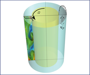
We study the flow developing between two concentric cylinders of axial length  $L_{z}$ with the inner, of radius $R_{i}$, rotating at constant angular velocity $\unicode[STIX]{x1D6FA}$ and the outer, of radius $R_{o}$, at rest. The flow is also axially driven by a pulsatile pressure gradient. The aim of the present study is to investigate the effects of the unsteady forcing on the base flow. The flow is governed by the incompressible Navier–Stokes equations, which, in primitive variables and dimensionless form, read
 $$\begin{eqnarray}\frac{\unicode[STIX]{x2202}\boldsymbol{u}}{\unicode[STIX]{x2202}t}=-\unicode[STIX]{x1D735}p-{\mathcal{N}}\boldsymbol{u}+\frac{1}{Ta}{\mathcal{L}}\boldsymbol{u}+{\mathcal{F}},\quad \unicode[STIX]{x1D735}\circ \boldsymbol{u}=0,\end{eqnarray}$$
 with  $p$ the pressure and $\boldsymbol{u}=(u,v,w)^{\text{T}}$ the velocity vector.
The term  ${\mathcal{F}}=(\overline{{\mathcal{F}}}+\widetilde{{\mathcal{F}}}\sin (2\unicode[STIX]{x1D712}^{2}t/Ta),0,0)^{\text{T}}$ represents the pulsatile pressure gradient, with $\overline{{\mathcal{F}}}$ the mean component and $\widetilde{{\mathcal{F}}}$ the fluctuation. Within this normalization, the oscillation period is $T_{osc}=\unicode[STIX]{x03C0}Ta/\unicode[STIX]{x1D712}^{2}$, $Ta$ and $\unicode[STIX]{x1D712}$ being non-dimensional parameters defined below.
In (2.1)  ${\mathcal{N}}\boldsymbol{u}=(\boldsymbol{u}\boldsymbol{\cdot }\unicode[STIX]{x1D735})\boldsymbol{u}$ and ${\mathcal{L}}\boldsymbol{u}=\unicode[STIX]{x0394}\boldsymbol{u}$ indicate the convective and diffusive terms, respectively. The variables are made dimensionless using the tangential velocity of the inner cylinder $\unicode[STIX]{x1D6FA}R_{i}$ and the gap width $S=R_{o}-R_{i}$. The geometry of the system is fully defined by two quantities, $\ell _{z}=L_{z}/S$ and $\unicode[STIX]{x1D702}=R_{i}/R_{o}$. The dynamics of the base flow is characterized by only two dimensionless parameters, the Taylor number and Reynolds number,
 $$\begin{eqnarray}Ta=\frac{\unicode[STIX]{x1D6FA}R_{i}S}{\unicode[STIX]{x1D708}},\quad Re=\frac{U_{b}S}{\unicode[STIX]{x1D708}},\end{eqnarray}$$
 with  $U_{b}$ the mean bulk axial velocity and $\unicode[STIX]{x1D708}$ the kinematic viscosity of the fluid. The axial flow unsteadiness is parametrized by the quantities
 $$\begin{eqnarray}\unicode[STIX]{x1D712}=\frac{S}{\unicode[STIX]{x1D6FF}},\quad \unicode[STIX]{x1D6FD}=\frac{U_{0}}{U_{b}},\end{eqnarray}$$
 where  $\unicode[STIX]{x1D6FF}=\sqrt{2\unicode[STIX]{x1D708}/\unicode[STIX]{x1D714}}$ is the Stokes layer thickness with $\unicode[STIX]{x1D714}$ the dimensional pulsation and $U_{0}$ the amplitude of the periodic modulation of the bulk axial velocity.
For sufficiently small values of the Reynolds and Taylor numbers, the axial and azimuthal velocity components are decoupled (parallel flow) and the dimensionless velocity of the base flow reads
 $$\begin{eqnarray}\left.\begin{array}{@{}c@{}}\displaystyle u(r)=u_{ann}(r)=2\frac{Re}{Ta}\frac{[1-r^{2}(1-\unicode[STIX]{x1D702})^{2}]\log \unicode[STIX]{x1D702}-\log [r(1-\unicode[STIX]{x1D702})](1-\unicode[STIX]{x1D702}^{2})}{(1+\unicode[STIX]{x1D702}^{2})\log \unicode[STIX]{x1D702}+(1-\unicode[STIX]{x1D702}^{2})},\\ \displaystyle v(r)=0,\\ \displaystyle w(r)=w_{Cou}(r)=\frac{\unicode[STIX]{x1D702}}{1-\unicode[STIX]{x1D702}^{2}}\left[\frac{1}{r(1-\unicode[STIX]{x1D702})}-r(1-\unicode[STIX]{x1D702})\right],\end{array}\right\}\end{eqnarray}$$ $r=R/S$ being the scaled radial coordinate.
The unsteady pressure gradient induces an axial oscillating velocity component whose analytical expression, under the assumption of parallel flow, is the real part of the following complex function (Tsangaris Reference Tsangaris1984):
 $$\begin{eqnarray}\displaystyle & & \displaystyle \hspace{-11.99998pt}u_{osc}(r,t)=u_{Stokes}(r,t)=-\frac{\text{i}(1-\unicode[STIX]{x1D702})^{2}}{2\unicode[STIX]{x1D712}^{2}}\unicode[STIX]{x1D6FD}\frac{Re}{Ta}\text{e}^{\text{i}\unicode[STIX]{x1D714}t}\nonumber\\ \displaystyle & & \displaystyle \hspace{-8.50006pt}\times \left\{1-\frac{\left[\text{K}_{0}\left({\displaystyle \frac{\sqrt{2\text{i}}\unicode[STIX]{x1D702}}{1-\unicode[STIX]{x1D702}}}\unicode[STIX]{x1D712}\right)-\text{K}_{0}\left({\displaystyle \frac{\sqrt{2\text{i}}}{1-\unicode[STIX]{x1D702}}}\unicode[STIX]{x1D712}\right)\right]\text{I}_{0}(\sqrt{2\text{i}}\unicode[STIX]{x1D712}r)+\left[\text{I}_{0}\left({\displaystyle \frac{\sqrt{2\text{i}}}{1-\unicode[STIX]{x1D702}}}\unicode[STIX]{x1D712}\right)-\text{I}_{0}\left({\displaystyle \frac{\sqrt{2\text{i}}\unicode[STIX]{x1D702}}{1-\unicode[STIX]{x1D702}}}\unicode[STIX]{x1D712}\right)\right]\text{K}_{0}(\sqrt{2\text{i}}\unicode[STIX]{x1D712}r)}{\text{I}_{0}\left({\displaystyle \frac{\sqrt{2\text{i}}}{1-\unicode[STIX]{x1D702}}}\unicode[STIX]{x1D712}\right)\text{K}_{0}\left({\displaystyle \frac{\sqrt{2\text{i}}\unicode[STIX]{x1D702}}{1-\unicode[STIX]{x1D702}}}\unicode[STIX]{x1D712}\right)-\text{I}_{0}\left({\displaystyle \frac{\sqrt{2\text{i}}\unicode[STIX]{x1D702}}{1-\unicode[STIX]{x1D702}}}\unicode[STIX]{x1D712}\right)\text{K}_{0}\left({\displaystyle \frac{\sqrt{2\text{i}}}{1-\unicode[STIX]{x1D702}}}\unicode[STIX]{x1D712}\right)}\right\},\nonumber\\ \displaystyle & & \displaystyle\end{eqnarray}$$
 where  $\text{i}=\sqrt{-1}$ is the imaginary unit, $\text{I}_{0}(\cdot )$ and $\text{K}_{0}(\cdot )$ are the modified Bessel functions of the first and second kind, respectively. There is no effect of the oscillating pressure gradient on the radial and azimuthal velocity components, i.e. $v_{osc}(r,t)=w_{osc}(r,t)=0$.
Theoretical results for the stability of pulsating SPF to axisymmetric or non-axisymmetric disturbances, to the best of our knowledge, have not been obtained yet. Thus the existence of a multiplicity of stable states coexisting at the same points of the parameter space, such as those embedded in the Eckhaus bands, is unknown. In narrow-gap geometries, the already mentioned stability studies on the SPF indicated that the critical Taylor number is one order of magnitude smaller than the present one (value defined below). Likewise, in the oscillating case, the results of Hu & Kelly (Reference Hu and Kelly1995) are limited to Taylor number significantly smaller than the present one.
Considering that a time-harmonic axial pressure gradient with zero mean has a stabilizing effect on the Taylor–Couette flow (Hu & Kelly Reference Hu and Kelly1995), it is conjectured that such a stabilization could occur also in the pulsatile case. According to the above arguments, it is expected that the envelope of the SPF reverse transition will be modified by the addition of a time-harmonic oscillating component to the mean pressure gradient. This transition entails a torque reduction and therefore it might be relevant for engineering applications.
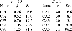
The possibility to induce a reverse transition in a pulsating SPF is the main aim of the present study, which, in particular, focuses on the effects of the unsteady forcing on an SPF at moderate Taylor number in a narrow-gap configuration. Starting from the available DNS data of Manna & Vacca (Reference Manna and Vacca2009), a set of new DNS data has been produced for  $Ta=1500$, $Re=250$ and $\unicode[STIX]{x1D702}=0.98$. Note that this base flow state lies significantly far from the aforementioned reverse transition process lower bound $Re_{RT}$. The effects on the base flow of both the oscillating amplitude (at a fixed $\unicode[STIX]{x1D712}$ value) and frequency (at approximately constant $\unicode[STIX]{x1D6FD}$ value) have been explored in terms of global and local features. Table 1 reports the investigated parameter space in the $\unicode[STIX]{x1D6FD}$– $\unicode[STIX]{x1D712}$ plane, where it can be seen that two series of five simulations each, one at constant frequency ( $\unicode[STIX]{x1D712}=10$, CF simulations) and one at constant amplitude ( $\unicode[STIX]{x1D6FD}\simeq 1$, CA simulations), are performed. Finally, for the sake of comparison two cases, for pure Taylor–Couette flow (TCF, $Ta=1500$) and spiral Poiseuille flow (SPF, $Ta=1500$ and $Re=250$), have been simulated and used as reference to isolate the oscillating forcing effects.
The values of the oscillating Reynolds number ( $Re_{\unicode[STIX]{x1D6FF}}=U_{0}\unicode[STIX]{x1D6FF}/\unicode[STIX]{x1D708}=\unicode[STIX]{x1D6FD}Re/\unicode[STIX]{x1D712}$) given in table 1 ensure that, as far as the purely oscillatory component is concerned, all simulations are in laminar flow conditions.
Table 1. Run matrix of the simulated cases ( $Ta=1500$, $Re=250$). CF, constant frequency; CA, constant amplitude.
We anticipate that, depending on the  $\unicode[STIX]{x1D6FD}$– $\unicode[STIX]{x1D712}$ pair, the pulsation can produce a turbulent to laminar reverse transition of the flow (large $\unicode[STIX]{x1D6FD}$ or small $\unicode[STIX]{x1D712}$ values) or it will not alter the time-averaged flow features of the base flow (small $\unicode[STIX]{x1D6FD}$ or large $\unicode[STIX]{x1D712}$ values). In between the above two, a third region in the $(\unicode[STIX]{x1D6FD},\unicode[STIX]{x1D712})$ plane exists in which the flow field is modified by the pulsation. To clarify the above concept, we graphically present in figure 1(b) the run matrix together with the qualitative boundaries of the above-mentioned regimes. In figure 1(b) the three regimes are respectively denoted as: LBP (laminarized by pulsation), UBP (unaffected by pulsation) and ABP (affected by pulsation). In order to better define the boundary between the UBP and ABP regimes, two additional simulations at variable $\unicode[STIX]{x1D6FD}$ and $\unicode[STIX]{x1D712}$ (AS1: $\unicode[STIX]{x1D6FD}=0.47$, $\unicode[STIX]{x1D712}=20$, $Re_{\unicode[STIX]{x1D6FF}}=5.9$; and AS2: $\unicode[STIX]{x1D6FD}=0.79$, $\unicode[STIX]{x1D712}=30$, $Re_{\unicode[STIX]{x1D6FF}}=6.6$) have been run and included in figure 1(b).

Figure 1. (a) Sketch of the problem. (b) The  $\unicode[STIX]{x1D6FD}{-}\unicode[STIX]{x1D712}$ phase space, showing the approximate boundaries between different flow regimes: ▸, UBP; ●, ABP; ▪, LBP.
3 Numerical method and computational set-up
Equations (2.1) have been numerically solved by a pressure correction scheme (van Kan Reference van Kan1986) and a spectral multi-domain technique (Manna & Vacca Reference Manna and Vacca1999). As customary in fully resolved turbulent wall-bounded flows, the diffusive terms have been treated implicitly in time using a second-order Crank–Nicolson scheme. Conversely, the convective operator, rewritten in skew-symmetric form, has been discretized explicitly using a second-order Adams–Bashforth scheme. A blended Fourier decomposition for the homogeneous (axial and azimuthal) directions has been applied, while a pseudo-spectral Chebyshev discretization has been used in the radial direction. Moreover, the efficiency of the whole algorithm has been improved through a multi-domain approach with patching interfaces (Manna, Vacca & Deville Reference Manna, Vacca and Deville2004). The solver has been extensively validated in both steady (Manna & Vacca Reference Manna and Vacca2001, Reference Manna and Vacca2009) and unsteady (Manna, Vacca & Verzicco Reference Manna, Vacca and Verzicco2012, Reference Manna, Vacca and Verzicco2015) turbulent simulations.
Similarly to Manna & Vacca (Reference Manna and Vacca2009), the extent of the computational domain has been limited in both the axial and azimuthal directions, exploiting the flow periodicity. Relying on the results by Manna & Vacca (Reference Manna and Vacca2009) assessing the adequacy of the box size, the lengths in the axial and in the azimuthal (referred to the mean radius) directions have been fixed equal to  $\ell _{z}=8$ and $\ell _{\unicode[STIX]{x1D703}}=(\unicode[STIX]{x03C0}/9)(1+\unicode[STIX]{x1D702})/(1-\unicode[STIX]{x1D702})\approx 35$, respectively.
The discretization of the computational domain relies on the use of four subdomains, each of which has 14 Chebyshev modes, in the radial direction. In order to improve the near-wall resolution, the radial extents of the innermost and outermost subdomains have been reduced to  $S/6$, while the sizes of the two central subdomains are equal to $S/3$. The numbers of Fourier modes in the axial and azimuthal directions have been fixed equal to 128 and 256, respectively. The adequacy of the computational box size and the grid convergence checks are given in the next section (§ 4).
No-slip boundary conditions for all velocity components have been prescribed at both cylinder surfaces, while periodicity has been imposed in the axial and azimuthal directions. The time step has been set equal to  $1.3\times 10^{-2}$ dimensionless units for all cases except for the highest-frequency case (CA1) in which the time step has been reduced to $1.3\times 10^{-3}$.
All simulations have been initiated starting from the database of Manna & Vacca (Reference Manna and Vacca2009) and, for each case, the triplet  $\overline{{\mathcal{F}}},\widetilde{{\mathcal{F}}},2\unicode[STIX]{x1D712}^{2}/Ta$ has been devised in order to obtain the parameters of table 1. Owing to the nonlinear dependence of the velocity field on the forcing ${\mathcal{F}}$, a triplet cannot be determined a priori to yield a precise value of $\unicode[STIX]{x1D6FD}$. Accordingly, the determination of the appropriate ${\mathcal{F}}$ relies on extrapolations from close flow states and iterative attempts. For the sake of completeness and to enable the reproduction of the present database, we detail in table 2 the exact $\unicode[STIX]{x1D6FD}$ values used in CA cases.
Table 2. Exact  $\unicode[STIX]{x1D6FD}$ values used in the computations in the constant-amplitude cases.

In order to obtain converged phase-averaged statistics, each case has been run for a large enough number of periods. In more detail, for the cases at the dimensionless frequencies  $\unicode[STIX]{x1D712}=10$, 20, 30 and 40 a number of cycles of 200, 250, 400 and 600, respectively, has been simulated; while for the SPF (with only the constant axial pressure gradient $\overline{{\mathcal{F}}}$) and the TCF cases, the statistics converge faster and the simulations were stopped when the root-mean-square (r.m.s.) velocity profiles and spectra did not show variations (900 and 1800 convective time units).
As customary in turbulent flows, the quantities enclosed in angle brackets  $\langle \bullet \rangle$ are phase-averaged within the oscillating period as well as over the two homogeneous directions $z$ and $\unicode[STIX]{x1D703}$. The overline $\bar{\bullet }$ is used to indicate (multi-)cycle-averaged data. The modulation within the cycle is therefore evaluated by the difference between phase- and cycle-averaged quantities and it is written as $\widetilde{\bullet }=\langle \bullet \rangle -~\bar{\bullet }$. The phase averages have been sampled at eight equally spaced intervals within the period, so that two adjacent samples are $T_{osc}/8=\unicode[STIX]{x03C0}Ta/(8\unicode[STIX]{x1D712}^{2})$ far apart. We denote by $\unicode[STIX]{x1D719}_{i}=(i-1)2\unicode[STIX]{x03C0}/8$, with $i=1,\ldots ,8$, the corresponding phases. The deviations of the instantaneous quantities from their phase-averaged counterpart are indicated by a prime symbol $\bullet ^{\prime }$.
Finally, the quantities averaged in the azimuthal and axial directions retain only the radial dependence; for the ease of representation, their profiles are plotted using the distance from the inner cylinder normalized by the gap  $y=(R-R_{i})/S$.
4 Convergence checks
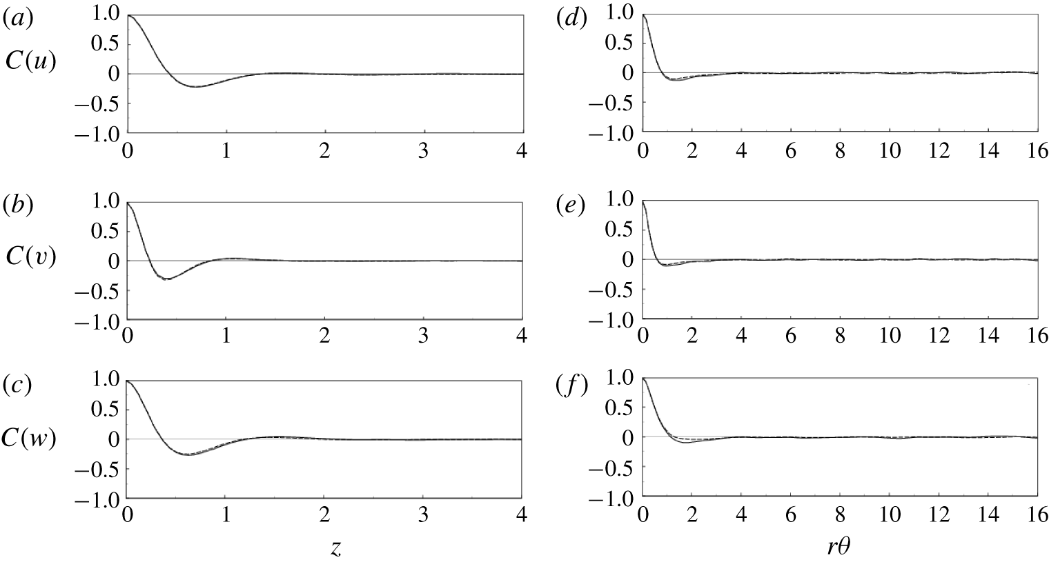
Figure 2. Velocity spatial correlations at  $y=0.11$: (a–c) $z$ direction, (d–f) $\unicode[STIX]{x1D703}$ direction; (a,d) $z$ component, (b,e) $r$ component, (c,f) $\unicode[STIX]{x1D703}$ component; ——, SPF case; - - - -, CF2 case. Note that only half of the domain length is reported in each plot, since, owing to periodicity, the correlation must be symmetric about the midpoint.
The adequacy of the axial ( $\ell _{z}$) and azimuthal ( $\ell _{\unicode[STIX]{x1D703}}$) lengths of the computational domain has been demonstrated through the analysis of the two-point correlation at $y=0.11$ for all the velocity components reported in figure 2. Figure 2(a) (respectively figure 2b) refers to the axial (respectively azimuthal) direction. Only the SPF and CF2 cases are shown, the latter being assumed representative of the run matrix of table 1. Clearly the box size is large enough to accommodate the largest coherent structures in both directions, as can be appreciated from the spatial correlations that decay to zero already for distances smaller than one-quarter of the domain length. This indicates that the flow dynamics is not significantly affected by the size of the computational box. We note that these results are not much different from those of the SPF, and therefore we can conclude that the temporal modulation is seen to affect only marginally the size and shape of the near-wall coherent structures, at least for the parameter range explored in this paper.
The effects of the spatial resolution have been quantified through a grid refinement study, conducted firstly in the homogeneous directions  $z$ and $\unicode[STIX]{x1D703}$, keeping fixed the $\ell _{z}$ and $\ell _{\unicode[STIX]{x1D703}}$ lengths and the number of radial modes, in each subdomain. The number of Fourier modes in the two homogeneous directions has been separately increased by a factor $1.5$. Figure 3 reports the one-dimensional power spectra of all velocity components versus $k_{z}$ and $k_{\unicode[STIX]{x1D703}}$ at $y=0.11$, for both the SPF and the CF2 cases. The spectra are perfectly smooth and the fine-grid data overlap with those for the coarse one at all wavenumbers, without any energy pile-up at the highest wavenumber, thus confirming that the simulations are solving all the energy-containing scales. The convergence in the radial direction has been tested by increasing the number of Chebyshev modes in each subdomain from 12 to 15 while keeping fixed the number of Fourier modes. The study has been carried out with reference to the CA1 case in which the largest velocity gradients close to the walls are expected. Indeed, in this case, the Stokes layer is a small fraction of the near-wall subdomains’ radial extent. Figure 4 reports the comparison of cycle-averaged r.m.s. velocity profiles obtained with the refined and standard grids, showing only negligible differences. Accounting for the exponential error decay of the present algorithm and the degree of agreement for different resolutions and domain dimensions, the quality of the results is considered satisfactory.

Figure 3. Velocity power spectra at  $y=0.11$: (a,b) $z$ direction, (c,d) $\unicode[STIX]{x1D703}$ direction; (a,c) SPF case, (b,d) CF2 case; ——, standard mesh; - - - -, refined mesh.

Figure 4. Radial profiles of the cycle-averaged r.m.s. velocity components for the case CA1 ( $\unicode[STIX]{x1D712}=40$, $\unicode[STIX]{x1D6FD}=1$): ——, for the refined grid; - - - -, for the standard grid.
5 Results
5.1 Global parameters
The overall flow dynamics is initially quantified by the driving torque coefficient defined as
 $$\begin{eqnarray}C_{\unicode[STIX]{x1D70F}}=\overline{\unicode[STIX]{x1D70F}}_{r\unicode[STIX]{x1D703},i}=-\frac{r}{Ta}\frac{\text{d}}{\text{d}r}\left(\frac{\overline{w}}{r}\right)_{r_{i}},\end{eqnarray}$$
 where  $\overline{\unicode[STIX]{x1D70F}}_{r\unicode[STIX]{x1D703},i}$ is the surface- and time-averaged azimuthal component of the wall shear stress at the inner cylinder. Likewise the axial pressure gradient is defined as
 $$\begin{eqnarray}\frac{\unicode[STIX]{x0394}\overline{p}}{\ell _{z}}=2\frac{\overline{\unicode[STIX]{x1D70F}}_{rz,o}-\overline{\unicode[STIX]{x1D70F}}_{rz,i}\unicode[STIX]{x1D702}}{1+\unicode[STIX]{x1D702}},\end{eqnarray}$$
 with  $\overline{\unicode[STIX]{x1D70F}}_{rz,i/o}=((\text{d}\overline{u}/\text{d}r)/Ta)_{i/o}$ the analogous axial components of the shear stress at the inner/outer cylinders, and it is related to the axial friction coefficient $\unicode[STIX]{x1D706}$ by
 $$\begin{eqnarray}\unicode[STIX]{x1D706}=4\frac{\unicode[STIX]{x0394}\overline{p}}{\ell _{z}}\frac{Ta^{2}}{Re^{2}}.\end{eqnarray}$$
In the following, in order to disentangle the effects of amplitude and frequency of the oscillation, the results are presented as a function of only one parameter while maintaining the other constant (see table 1).
Figure 5(a) presents the torque and axial friction coefficients, normalized by the corresponding SPF values, as a function of  $\unicode[STIX]{x1D6FD}$ (CF cases). For increasing $\unicode[STIX]{x1D6FD}$, the torque coefficient continuously decreases from a value close to $C_{\unicode[STIX]{x1D70F},SPF}$ down to the fully laminar Taylor–Couette value for $\unicode[STIX]{x1D6FD}=1.25$ (CF5 case), thus losing ${\approx}60\,\%$ of its initial magnitude. A similar trend is found for the axial friction coefficient $\unicode[STIX]{x1D706}/\unicode[STIX]{x1D706}_{SPF}$, leading to ${\approx}30\,\%$ reduction and yielding an axial friction drop approximately half that of the torque.

Figure 5. Torque and axial friction coefficients: (a)  $\unicode[STIX]{x1D712}=10$, (b) $\unicode[STIX]{x1D6FD}\sim 1$.
The decrease of torque and friction coefficient is also evident from the azimuthal and axial mean velocity profiles whose wall gradients keep decreasing for increasing  $\unicode[STIX]{x1D6FD}$ down to the fully laminar values. This point is addressed and further discussed in § 5.2.
This laminarization process can be explained by associating the pulsating motion to the instantaneous Reynolds number  $(Re_{m})$ computed with $U_{m}=(\unicode[STIX]{x1D6FD}+1)U_{b}$ as velocity scale. Indeed, previous studies (Yamada Reference Yamada1962a,Reference Yamadab; Manna & Vacca Reference Manna and Vacca2009) have shown that the steady flow at $Ta=1500$ undergoes laminarization in the range $400\sim Re_{R}\leqslant Re\leqslant Re_{D}\sim 800$. Under pulsating conditions, however, this reverse transition takes place at higher $Re$ and, although the precise value of $Re_{R}$ is unknown, it has been seen to be larger than $Re_{m}=513$ (CF4 case) and smaller than $Re_{m}=563$ (CF5 case).
Figure 5(b), the counterpart of figure 5(a) for the CA cases, shows a similar behaviour for both torque and axial friction coefficients when, for a fixed amplitude value, the pulsation frequency is reduced. For sufficiently high frequencies  $(\unicode[STIX]{x1D712}>40)$, the flow appears to be insensitive to the oscillating component, although the maximum instantaneous Reynolds number is $Re_{m}=500$, and therefore significantly larger than $Re_{R}$. Lowering the frequency of the axial oscillating pressure gradient leads to a progressive reduction of both torque and axial friction coefficients, which recover their corresponding laminar values at $\unicode[STIX]{x1D712}=2.5$.
Since all CA simulations are characterized by a maximum instantaneous Reynolds number larger than  $Re_{R}$, while the reverse transition occurs only for the longest oscillating period, $\unicode[STIX]{x1D712}=2.5$, it is conjectured that the extent of the time window in which $Re_{m}$ exceeds $Re_{R}$ plays a key role in determining the reverse transition.
It is worth mentioning that the relaminarizing effect of an oscillating forcing might be not only a peculiarity of the SPF but rather a more general effect. In fact, the possibility to modify the transition boundaries either increasing the amplitude or decreasing the frequency of the pulsation has also been reported for pipe flow by Xu et al. (Reference Xu, Warnecke, Song, Ma and Hof2017) and Xu & Avila (Reference Xu and Avila2018).
In figure 6 we report some instantaneous  $r$–
$r$– $z$ slices of representative flows in order to give an idea of how the structures are affected by the mean and pulsating axial forcing. While the comparison between TCF and SPF cases clearly shows that a time-constant axial flow breaks the regularity and decreases the strength of the Taylor rolls, the situation in the pulsating cases is different. Considering the small-amplitude pulsating case (CF1), figure 6(c) shows an instantaneous realization whose phase angle has been selected in such a way that the bulk velocity equals the SPF value. The crude comparison between figures 6(b) and 6(c) reveals that the flow features of SPF and CF1 are similar, a fact that agrees well with the global parameter results reported in figure 5. In the large-amplitude pulsating case, i.e. CF4 (see figure 6d), the number of Taylor rolls and their strength appear to be reduced when compared to the CF1 case, at the same phase angle.

Figure 6. Instantaneous snapshots in an  $r$–
$r$– $z$ plane of the $w$ velocity component with the velocity vector overlaid: (a) TCF, (b) SPF, (c) CF1, (d) CF4. The cases CF1 and CF4 have been sampled at the phase $\unicode[STIX]{x1D6F7}_{1}=0$ so that panels (b), (c) and (d) are for the same $U_{b}$. Only half of the vertical domain is reported for clarity.
Inspecting the in-cycle evolution of the large-scale structures (results not shown), it appears that their dynamics is highly phase-dependent and therefore their characterization cannot be inferred from a single instantaneous snapshot. For this reason in figure 7 we show the one-dimensional power spectra for all velocity components in the azimuthal wavenumber space ( $k_{\unicode[STIX]{x1D703}}=2\unicode[STIX]{x03C0}k/\ell _{\unicode[STIX]{x1D703}}$) at $y=0.11$ for the TCF, SPF, CF1 and CF4 cases. Comparing TCF with SPF reveals that a time-constant axial flow reduces the magnitude of the Taylor rolls, as can be inferred from the energy content at small wavenumbers, and strengthens the smaller scales, i.e. high wavenumbers. As already mentioned, there are only marginal differences between SPF and CF1. Conversely, the CF4 case strongly differs from SPF at both small and large scales and resembles closely TCF.
The complexity of the interaction of those scales motivates the use of cycle- and phase-averaged statistics for the analysis of the results presented in the remaining part of the paper.

Figure 7. Velocity power spectra in the azimuthal direction: (a)  $z$ component, (b) $r$ component, (c) $\unicode[STIX]{x1D703}$ component; black, TCF; red, SPF; green, CF1; and blue, CF4.
It is worthwhile to note that, even if in the reverse transition region of the  $\unicode[STIX]{x1D6FD}$– $\unicode[STIX]{x1D712}$ space both $C_{\unicode[STIX]{x1D70F}}$ and $\unicode[STIX]{x1D706}$ decrease with respect to the steady flow values (figure 5), additional power is still needed to drive the oscillating axial flow component and this might make up for, or even overcome, the savings of the steady part.
The time-mean input power required to keep the inner cylinder rotating and to ensure the prescribed (time-varying) flow rate is decomposed as follows:
 $$\begin{eqnarray}{\mathcal{P}}_{tot}={\mathcal{P}}_{\unicode[STIX]{x1D703}}+{\mathcal{P}}_{z}.\end{eqnarray}$$
 Using (5.1),  ${\mathcal{P}}_{\unicode[STIX]{x1D703}}$ can be expressed by
 $$\begin{eqnarray}{\mathcal{P}}_{\unicode[STIX]{x1D703}}=2\unicode[STIX]{x03C0}C_{\unicode[STIX]{x1D70F}}\frac{\unicode[STIX]{x1D702}}{1-\unicode[STIX]{x1D702}}\ell _{z},\end{eqnarray}$$
while the power associated with the axial flow reads
 $$\begin{eqnarray}{\mathcal{P}}_{z}=\overline{{\mathcal{P}}}_{z}+\widetilde{{\mathcal{P}}}_{z}=\frac{\unicode[STIX]{x03C0}}{4}\unicode[STIX]{x1D706}\frac{Re^{3}}{Ta^{3}}\frac{1+\unicode[STIX]{x1D702}}{1-\unicode[STIX]{x1D702}}\ell _{z}+2\unicode[STIX]{x03C0}\ell _{z}\widetilde{{\mathcal{F}}}\int _{\unicode[STIX]{x1D702}/(1-\unicode[STIX]{x1D702})}^{1/(1-\unicode[STIX]{x1D702})}[\overline{\sin (\unicode[STIX]{x1D714}t)\widetilde{u}(r,t)}]r\,\text{d}r.\end{eqnarray}$$
 Figure 8 shows the ratio between  ${\mathcal{P}}_{tot}$ and the power of the spiral flow ( ${\mathcal{P}}_{tot,SPF}$), in the $\unicode[STIX]{x1D6FD}=\text{const.}$ and $\unicode[STIX]{x1D712}=\text{const.}$ cases. The ${\mathcal{P}}_{tot,SPF}$ value is evaluated through (5.4)–(5.6) with $C_{\unicode[STIX]{x1D70F}}=C_{\unicode[STIX]{x1D70F},SPF}$, $\unicode[STIX]{x1D706}=\unicode[STIX]{x1D706}_{SPF}$ and $\widetilde{{\mathcal{P}}}_{z}=0$. Moreover, in both panels the individual contributions of ${\mathcal{P}}_{z}$ and ${\mathcal{P}}_{\unicode[STIX]{x1D703}}$ to the total power are also reported.

Figure 8. Power input at (a)  $\unicode[STIX]{x1D712}=10$ and (b) $\unicode[STIX]{x1D6FD}\sim 1$: ▸, ${\mathcal{P}}_{z}/{\mathcal{P}}_{tot,SPF}$; ▪, ${\mathcal{P}}_{\unicode[STIX]{x1D703}}/{\mathcal{P}}_{tot,SPF}$; and ●, ${\mathcal{P}}_{tot}/{\mathcal{P}}_{tot,SPF}$.
At small oscillating amplitude, i.e.  $\unicode[STIX]{x1D6FD}=0.25$, the additional contribution of the unsteady term to the total power is negligible and the ratio ${\mathcal{P}}_{tot}/{\mathcal{P}}_{tot,SPF}$ remains very close to one (figure 8a). The small reduction of the power ratio stems from the minor change in the $\unicode[STIX]{x1D706}$ value already documented in figure 5. At larger $\unicode[STIX]{x1D6FD}$, there is an appreciable reduction of the total power, which is to be mainly attributed to the changes of the torque coefficient generated by the pulsation. This reduction is progressive and reaches ${\sim}60\,\%$ at $\unicode[STIX]{x1D6FD}=1.25$, when the reverse transition process is completed.
The effects of the frequency at constant amplitude are different (figure 8b). At large oscillating frequency, i.e.  $\unicode[STIX]{x1D712}=40$, the power contribution required to keep the pulsation running is large and it reaches ${\sim}40\,\%$ of the base power. Reducing the oscillating frequency results in a power reduction associated with both the smaller number of cycles per unit time and the resistance and torque reduction previously discussed in figure 5(b). As before, the power reduction is progressive and it reaches a remarkable ${\sim}50\,\%$ at $\unicode[STIX]{x1D712}=2.5$, when the reverse transition is attained.
5.2 Mean velocity profiles
In this subsection we discuss the multi-cycle-averaged radial profiles of azimuthal and axial velocity.
Figure 9 shows the effects of the amplitude (figure 9a) and frequency (figure 9b) of the oscillating forcing on the  $\overline{w}(y)$ profile. For the sake of clarity, the pure TCF and SPF profiles are reported in the same panels. The comparison of TCF with SPF cases shows less intense gradients in the latter owing to the attenuation of the Taylor vortices produced by the constant axial pressure gradient (Manna & Vacca Reference Manna and Vacca2009). Initially, when the pulsating component is introduced, both the CA1 and CF1 simulations coincide with the reference SPF, thus showing no effect of the unsteadiness, in both global and local terms.

Figure 9. Cycle-averaged azimuthal velocity profiles: (a)  $\unicode[STIX]{x1D712}=10$, (b) $\unicode[STIX]{x1D6FD}\sim 1$; - - - -, TCF; ——, SPF; ○, laminar solution. Full curves are as follows in panel (a) (panel (b), respectively): orange, CA1 (CF1); green, CA2 (CF2); blue, CA3 (CF3); cyan, CA4 (CF4); violet, CA5 (CF5).
However, either by increasing  $\unicode[STIX]{x1D6FD}$ or reducing $\unicode[STIX]{x1D712}$, the velocity profiles tend to the Couette flow (equations (2.4)) via a smooth process until, for $\unicode[STIX]{x1D6FD}=1.25$ (CF5 case) or $\unicode[STIX]{x1D712}=2.5$ (CA5 case), the reverse transition has occurred and the collapse is complete. The multi-cycle-averaged axial velocity profiles (figure 10) show a similar behaviour.

Figure 10. Cycle-averaged axial velocity profiles: (a)  $\unicode[STIX]{x1D712}=10$, (b) $\unicode[STIX]{x1D6FD}\sim 1$. Line styles as in figure 9.
With the aim of further analysing the interaction between the base SPF and the oscillating flow, in figures 11–13 we report the modulation of the axial velocity component across the gap compared with the analytical solution  $u_{Stokes}$, given by (2.5).
In the CF1 case (figure 11a), at all phase angles, the  $\widetilde{u}$ radial distribution shows the largest deviations from $u_{Stokes}$, especially in the core region, where they can be as large as 15 % of the local $u_{Stokes}$ value. Yet, the cycle-averaged velocity profiles are indistinguishable from the SPF solution (figures 9 and 10), thus implying that the oscillating and the mean flows are only one-way-coupled. However, increasing the amplitude of the oscillation ( $\unicode[STIX]{x1D6FD}$) alters the mutual interaction between the two flows in a complex manner. In fact, the unexpected one-way coupling becomes two-way with the oscillating forcing that increasingly affects the cycle-averaged axial and azimuthal velocity fields and, concurrently, the influence of $\overline{u}$ and $\overline{w}$ on $\widetilde{u}$ weakens. This mutual interaction eventually leads to a complete flow laminarization ( $\unicode[STIX]{x1D6FD}=1.25$), yielding a flow that can be described by the relations (2.4) and (2.5):
 $$\begin{eqnarray}u=u_{ann}+u_{Stokes},\quad v=0,\quad w=w_{Cou}.\end{eqnarray}$$
 For a given amplitude of the modulation ( $\unicode[STIX]{x1D6FD}$), the effect of the oscillating frequency ( $\unicode[STIX]{x1D712}$) on the cycle-averaged velocity $\widetilde{u}$ is shown in figures 11(b), 12(b) and 13(a). At the highest frequency, CA1 case ( $\unicode[STIX]{x1D712}=40$), the oscillating motion is fully decoupled from the cycle-averaged velocity, which is described by the solution (2.5) (figure 12b). Likewise $\overline{u}$ and $\overline{w}$ coincide with the SPF profiles and thus they are also decoupled from $\widetilde{u}$ (see figures 9 and 10). This behaviour can be explained by the thickness of the Stokes layers, at the cylinders’ surfaces, which is a small fraction of the annular gap ( $\unicode[STIX]{x1D6FF}\simeq S/40$) at this very high frequency of the forcing. Under this condition, the unsteadiness is confined within these layers, while in the outside region the flow oscillates as a plug flow. On the other hand, decreasing the frequency down to $\unicode[STIX]{x1D712}=20$ thickens the Stokes layers and the interaction between the oscillating and the steady components strengthens, thus leading to a two-way-coupled regime. At $\unicode[STIX]{x1D712}=2.5$, the mutual interaction between the two velocity fields disappears and the fully decoupled solution (5.7) is again recovered.

Figure 11. Radial profiles of phase-averaged vertical velocity  $\widetilde{u}$ for (a) $\unicode[STIX]{x1D712}=10$, $\unicode[STIX]{x1D6FD}=0.25$; (b) $\unicode[STIX]{x1D712}=10$, $\unicode[STIX]{x1D6FD}=1.0$; black ——, laminar analytical solution; red - - - -, numerical solution.
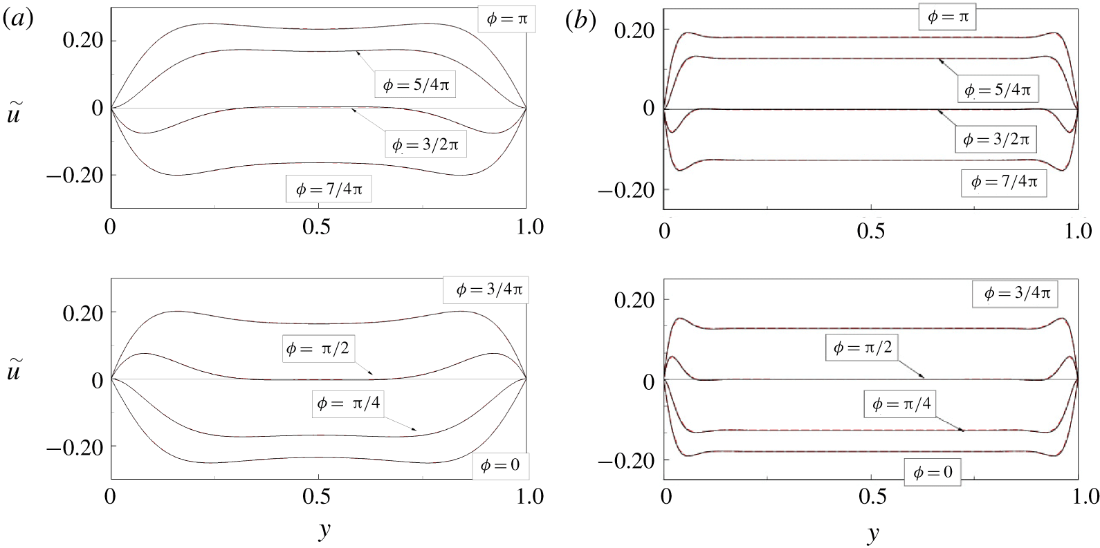
Figure 12. Radial profiles of phase-averaged vertical velocity  $\widetilde{u}$ for (a) $\unicode[STIX]{x1D712}=10$, $\unicode[STIX]{x1D6FD}=1.25$; (b) $\unicode[STIX]{x1D712}=40$, $\unicode[STIX]{x1D6FD}=1.0$. Lines as in figure 11.

Figure 13. Radial profiles of phase-averaged vertical velocity  $\widetilde{u}$ for (a) $\unicode[STIX]{x1D712}=20$, $\unicode[STIX]{x1D6FD}=1.0$; (b) $\unicode[STIX]{x1D712}=2.5$, $\unicode[STIX]{x1D6FD}=1.0$. Lines as in figure 11.
5.3 Reynolds stresses
Figure 14 (respectively figure 15) shows the effect of  $\unicode[STIX]{x1D6FD}$ (respectively $\unicode[STIX]{x1D712}$) on the main components of the cycle-averaged Reynolds stresses; the profiles of the TCF and SPF flows are reported for comparison. Taking as reference the pure Taylor–Couette flow, the main effect of the axial pressure gradient is the flattening of the $\text{r.m.s.}(u^{\prime })=\sqrt{\overline{u^{\prime }u^{\prime }}}$ profiles and the reduction of its magnitude in the bulk for increasing oscillation amplitude $\unicode[STIX]{x1D6FD}$ (respectively decreasing frequency $\unicode[STIX]{x1D712}$). The $\text{r.m.s.}(v^{\prime })$ and $\text{r.m.s.}(w^{\prime })$ profiles show a similar dynamics with a progressive reduction of the fluctuations as $\unicode[STIX]{x1D6FD}$ is increased and $\unicode[STIX]{x1D712}$ is reduced. Concerning the off-diagonal terms of the Reynolds stress tensors, $\overline{v^{\prime }w^{\prime }}$ is by far the most relevant and it exceeds the corresponding viscous term throughout the annular gap except close to the wall. Also the term $\overline{v^{\prime }w^{\prime }}$ is reduced by the axial pressure gradient and the scenario is consistent either with the reduction of the torque coefficient and with the weakening of the Taylor rolls already observed for the steady axial forcing (Manna & Vacca Reference Manna and Vacca2009).
With the unsteady axial forcing, a uniform reduction of all Reynolds stresses is observed, and the amount of reduction markedly depends on the values of the  $(\unicode[STIX]{x1D6FD},\unicode[STIX]{x1D712})$ pair. Indeed it is less evident for the CF1 and CA1 cases, while in the CA5 and CF5 simulations the loss of turbulent energy eventually leads to a complete flow laminarization.

Figure 14. Radial profiles of velocity  $\text{r.m.s.}(\unicode[STIX]{x1D712}=10)$: (a) axial, (b) radial, (c) azimuthal and (d) shear stress. Line styles as in figure 9 except for the violet line of cases CF5 and CA5 that is missing.
According to the above description, it appears that the oscillating pressure gradient produces a reduction of the Reynolds stresses and smoothes their distribution in the bulk. In order to better characterize the structure of turbulence, it might be useful to resort to the anisotropy index  $AI$ (Manna et al. Reference Manna, Vacca and Verzicco2012) that quantifies by a single scalar quantity the anisotropy of the Reynolds stress tensor (Lumley & Newman Reference Lumley and Newman1977). Figure 16 shows the $AI$ radial profiles for all cases of table 1 and, to aid the interpretation of the curves, we recall that the result is $AI=1$ for one-dimensional turbulence and $AI=0$ when turbulence is three-dimensional and isotropic.

Figure 15. Radial profiles of velocity  $\text{r.m.s.}(\unicode[STIX]{x1D6FD}\sim 1)$: (a) axial, (b) radial, (c) azimuthal and (d) shear stress. Line styles as in figure 9 except for the violet line of cases CF5 and CA5 that is missing.

Figure 16. Radial distributions of the anisotropy index: (a)  $\unicode[STIX]{x1D712}=10$, (b) $\unicode[STIX]{x1D6FD}\sim 1$. Line styles as in figure 9 except for the violet line of cases CF5 and CA5 that is missing.
A comparison of TCF and SPF immediately shows that the constant axial pressure gradient induces a considerable return to isotropy, especially in the bulk region, leading to a more oblate shape of the Reynolds stress spheroid (Simonsen & Krogstad Reference Simonsen and Krogstad2005). This result can be explained by considering the energy transfer from the azimuthal to the axial component produced by the tilting of the coherent vortices in the  $z$ direction. The analysis of the pressure–strain terms $\unicode[STIX]{x1D6F7}_{zz}$ and $\unicode[STIX]{x1D6F7}_{\unicode[STIX]{x1D703}\unicode[STIX]{x1D703}}$ of the turbulent energy budget (see (5.10)–(5.12) for the definition), performed in the next section, will allow us to quantify in detail the energy transfer rate mechanism among the different components.
Figure 16 also shows that the superposition of the pulsation leads to a progressive anisotropy increase in the core region with respect to the SPF case, especially for  $\unicode[STIX]{x1D6FD}$ larger than 0.5 and $\unicode[STIX]{x1D712}$ smaller than 20 or, in other words, the shape of the Reynolds stress spheroid becomes more prolate (Simonsen & Krogstad Reference Simonsen and Krogstad2005). Again, this result can be explained by the tilting of the Taylor rolls that alters the energy redistribution pattern (see § 5.4).
5.4 Turbulence energy budget
For the present problem, within the range of the investigated parameters, the azimuthal velocity component is the most relevant and the cycle-averaged energy budget for its fluctuations reads
 $$\begin{eqnarray}\displaystyle & & \displaystyle \underbrace{-2\overline{\langle v^{\prime }w^{\prime }\rangle \frac{\text{d}\langle w\rangle }{\text{d}r}}}_{P_{\unicode[STIX]{x1D703}}}\underbrace{-\frac{1}{r}\frac{\unicode[STIX]{x2202}(r\overline{v^{\prime }w^{\prime \,2}})}{\unicode[STIX]{x2202}r}-\frac{2}{r}\overline{v^{\prime }w^{\prime \,2}}}_{T}\nonumber\\ \displaystyle & & \displaystyle \quad +\underbrace{\frac{1}{Re}\left[\frac{1}{r}\frac{\unicode[STIX]{x2202}}{\unicode[STIX]{x2202}r}\left(r\frac{\unicode[STIX]{x2202}\overline{w^{\prime \,2}}}{\unicode[STIX]{x2202}r}\right)-\frac{2}{r^{2}}(\overline{w^{\prime \,2}}-\overline{v^{\prime \,2}})\right]}_{D}\nonumber\\ \displaystyle & & \displaystyle \quad -\,\underbrace{\frac{2}{r}\overline{p^{\prime }\frac{\unicode[STIX]{x2202}w^{\prime }}{\unicode[STIX]{x2202}\unicode[STIX]{x1D703}}}}_{\unicode[STIX]{x1D6F1}_{\unicode[STIX]{x1D703}}}\underbrace{-\frac{2}{Re}\left[\overline{\left(\frac{\unicode[STIX]{x2202}w^{\prime }}{\unicode[STIX]{x2202}z}\right)^{2}}+\overline{\left(\frac{\unicode[STIX]{x2202}w^{\prime }}{\unicode[STIX]{x2202}r}\right)^{2}}+\overline{\frac{1}{r^{2}}\left(\frac{\unicode[STIX]{x2202}w^{\prime }}{\unicode[STIX]{x2202}\unicode[STIX]{x1D703}}\right)^{2}}\right]}_{-\unicode[STIX]{x1D716}}=0.\end{eqnarray}$$
 As an aside we note that, following Touber & Leschziner (Reference Touber and Leschziner2012), the production term  $P_{\unicode[STIX]{x1D703}}$ could be further decomposed as
 $$\begin{eqnarray}P_{\unicode[STIX]{x1D703}}=-2\overline{v^{\prime }w^{\prime }}\frac{\text{d}\overline{w}}{\text{d}r}-2\overline{\widetilde{v^{\prime }w^{\prime }}\frac{\text{d}\widetilde{w}}{\text{d}r}},\end{eqnarray}$$
although here, unlike in Manna et al. (Reference Manna, Vacca and Verzicco2012), the interaction between phase-averaged stress and phase-averaged shear is negligible and it can therefore be ignored.
In order to highlight the main flow features for representative flow regimes, in figures 17(a,b) and 18(a), we report the energy budgets for the TCF, SPF and CA4 cases, respectively.

Figure 17. Azimuthal velocity fluctuation energy budget: (a) TCF case, (b) SPF case.  $Unb$ indicates the sum of all the terms on the left-hand side of (5.8).

Figure 18. (a) Azimuthal velocity fluctuation energy budget: CF4 case.  $Unb$ indicates the sum of all the terms on the left-hand side of (5.8). (b) Pressure–strain terms, radial profiles: red lines, TCF; blue lines, SPF; black lines, CF4.
For the base TCF case, the viscous diffusion  $D$ is negligible in most of the bulk, while at the mid-gap $\unicode[STIX]{x1D6F1}_{\unicode[STIX]{x1D703}}\simeq P_{\unicode[STIX]{x1D703}}$ and $-\unicode[STIX]{x1D716}\simeq T$ (figure 17a). The addition of the mean pressure gradient (figure 17b) produces opposite effects in the bulk and in the boundary layer regions. In the former, an increase in the magnitudes of $P_{\unicode[STIX]{x1D703}}$, $\unicode[STIX]{x1D6F1}_{\unicode[STIX]{x1D703}}$ and $\unicode[STIX]{x1D716}$ is observed while $T$ undergoes a reduction throughout the bulk, similarly to the diffusion $D$. In contrast, within the boundary layers ( $y\leqslant 0.1$ and $y\geqslant 0.9$), the axial pressure gradient produces a drop of the production $P_{\unicode[STIX]{x1D703}}$ with a corresponding reduction of $\unicode[STIX]{x1D716}$. Also the viscous diffusion $D$, playing a leading role at the wall, undergoes a major reduction, similarly to the transport term $T$. A relevant consequence of the altered budget is that, at the walls, the reduction of the dissipation $\unicode[STIX]{x1D716}$ is reflected in a decrease of the friction, which is consistent with the behaviour of the torque coefficient $C_{\unicode[STIX]{x1D70F}}$. In fact, following Eckhardt, Grossmann & Lohse (Reference Eckhardt, Grossmann and Lohse2007), it is possible to relate the cycle-volume-averaged dissipation $\unicode[STIX]{x1D716}$ to the torque coefficient through $C_{\unicode[STIX]{x1D70F}}=\unicode[STIX]{x1D716}S^{4}\unicode[STIX]{x1D70E}^{2}J_{L}/(\unicode[STIX]{x1D708}^{5}Ta)$ with $J_{L}=2\unicode[STIX]{x1D708}\unicode[STIX]{x1D6FA}R_{i}^{2}R_{o}^{2}/(R_{o}^{2}-R_{i}^{2})$ and $\unicode[STIX]{x1D70E}=[(1+\unicode[STIX]{x1D702})/(2\sqrt{\unicode[STIX]{x1D702}})]^{4}$, the laminar angular momentum flux and the ‘pseudo’-Prandtl number, respectively.
The above picture is confirmed also when the axial pressure gradient has an additional pulsating component (case CA4 of figure 18a) showing the same effect as for the SPF case but a smaller increase of  $-\unicode[STIX]{x1D6F1}_{\unicode[STIX]{x1D703}}$. Again the further reduced dissipation at the wall is congruous with the value of $C_{\unicode[STIX]{x1D70F}}$ of figure 5.
The production term  $P_{\unicode[STIX]{x1D703}}$ plays a key role. In fact, given the difference between Taylor ( $Ta=1500$) and Reynolds ( $Re=250$) numbers, the production terms in the budget of the axial and radial velocity components are at least one order of magnitude smaller than the analogous term ( $P_{\unicode[STIX]{x1D703}}$) for the azimuthal component. For this reason, the axial and radial components can only receive energy from the azimuthal component through the pressure–strain terms, which are analysed in the following. We decompose the pressure–velocity interaction terms $\unicode[STIX]{x1D6F1}_{\ast }$ into the pressure–strain $\unicode[STIX]{x1D6F7}_{\ast \ast }$ and pressure–diffusion $\unicode[STIX]{x1D6F9}_{\ast \ast }$ components as follows:
 $$\begin{eqnarray}\displaystyle & \displaystyle \unicode[STIX]{x1D6F1}_{z}=\unicode[STIX]{x1D6F7}_{zz}+\unicode[STIX]{x1D6F9}_{zz}=2\overline{p^{\prime }\frac{\unicode[STIX]{x2202}u^{\prime }}{\unicode[STIX]{x2202}z}}+0, & \displaystyle\end{eqnarray}$$
 $$\begin{eqnarray}\displaystyle & \displaystyle \unicode[STIX]{x1D6F1}_{r}=\unicode[STIX]{x1D6F7}_{rr}+\unicode[STIX]{x1D6F9}_{rr}=2\overline{p^{\prime }\frac{\unicode[STIX]{x2202}u_{r}^{\prime }}{\unicode[STIX]{x2202}r}}-2\overline{\frac{\unicode[STIX]{x2202}(p^{\prime }v^{\prime })}{\unicode[STIX]{x2202}r}}, & \displaystyle\end{eqnarray}$$
 $$\begin{eqnarray}\displaystyle & \displaystyle \unicode[STIX]{x1D6F1}_{\unicode[STIX]{x1D703}}=\unicode[STIX]{x1D6F7}_{\unicode[STIX]{x1D703}\unicode[STIX]{x1D703}}+\unicode[STIX]{x1D6F9}_{\unicode[STIX]{x1D703}\unicode[STIX]{x1D703}}=\frac{2}{r}\overline{p^{\prime }\left(\frac{\unicode[STIX]{x2202}w^{\prime }}{\unicode[STIX]{x2202}\unicode[STIX]{x1D703}}+v^{\prime }\right)}-2\overline{\frac{p^{\prime }v^{\prime }}{r}}. & \displaystyle\end{eqnarray}$$
 Of the two terms,  $\unicode[STIX]{x1D6F7}_{\ast \ast }$ is the one responsible for the inter-component energy transfer. Figure 18(b) shows the pressure–strain terms for the three cases TCF, SPF and CF4. Looking at TCF and SPF cases, it is evident that, in the bulk, the effect of a constant axial pressure gradient is to make $\unicode[STIX]{x1D6F7}_{\unicode[STIX]{x1D703}\unicode[STIX]{x1D703}}$ more negative while, concurrently, $\unicode[STIX]{x1D6F7}_{rr}$ and $\unicode[STIX]{x1D6F7}_{zz}$ increase. This implies that energy is drained from the azimuthal component towards the radial and axial ones, thus enhancing the isotropic character of turbulence as confirmed by the decrease of the anisotropy index $AI$ of figure 16. The superposition of a pulsating axial pressure gradient, however, seems to restore the $\unicode[STIX]{x1D6F7}_{\ast \ast }$ values in the bulk to values closer to the TCF and therefore to restore the anisotropy in the bulk. Of course, the latter effect will depend on the amplitude and frequency of the oscillation; nevertheless, the trend is monotonic, as evident from figure 16.
The dynamics in the boundary layer regions is quite different from that in the bulk, since, on moving from TCF to SPF and CF4, a progressive decrease of the energy transfer from the radial to the axial components is observed, thus indicating an altered energy balance among the velocity components. This behaviour is in fact confirmed both by the velocity fluctuations of figures 14 and 15 and by the smaller torque coefficient  $C_{\unicode[STIX]{x1D70F}}$ (figure 5) produced by the less turbulent boundary layers.
6 Conclusions
In this work, the effects of an oscillating pressure gradient on a spiral Poiseuille flow (SPF), at constant Reynolds number ( $Re=250$) and Taylor number ( $Ta=1500$) and in a narrow-gap geometry ( $\unicode[STIX]{x1D702}=0.98$ or $S/R_{0}=0.02$), have been investigated by direct numerical simulation (DNS) of the Navier–Stokes equations. The influence of both frequency and amplitude of the oscillating axial pressure gradient, expressed by the dimensionless parameters $\unicode[STIX]{x1D712}$ and $\unicode[STIX]{x1D6FD}$, respectively, on the flow dynamics has been analysed in terms of global and local parameters. Two complementary sets of simulations have been performed, one at constant oscillating frequency ( $\unicode[STIX]{x1D712}=10$) and variable amplitude ( $0\leqslant \unicode[STIX]{x1D6FD}\leqslant 1.25$) and the other keeping the amplitude constant ( $\unicode[STIX]{x1D6FD}=1$) and varying the frequency ( $2.5\leqslant \unicode[STIX]{x1D712}\leqslant 40$); all the cases have an oscillating Reynolds number $Re_{\unicode[STIX]{x1D6FF}}<100$ so that the oscillating flow component is in the laminar regime.
The results have shown that, depending on the pair  $\unicode[STIX]{x1D712}$– $\unicode[STIX]{x1D6FD}$, three different flow regimes can be attained: unaffected by pulsation (UBP), affected by pulsation (ABP) and laminarized by pulsation (LBP). In the first one, occurring for ( $\unicode[STIX]{x1D6FD}\leqslant 0.25$, $\unicode[STIX]{x1D712}=10$) or ( $\unicode[STIX]{x1D6FD}\simeq 1.0$, $\unicode[STIX]{x1D712}\geqslant 40$) the cycle-averaged statistics coincide with those of the SPF. In the LBP regime, attained for ( $\unicode[STIX]{x1D6FD}\geqslant 1.25$, $\unicode[STIX]{x1D712}=10$) or ( $\unicode[STIX]{x1D6FD}=1.0$, $\unicode[STIX]{x1D712}\leqslant 2.5$), the pulsation destroys the large-scale structures of the bulk, thus producing a reverse transition evidenced by the averaged profiles of both axial and azimuthal velocity components that recover the laminar distributions. Finally, in the intermediate ABP regime, the cycle-averaged statistics are initially close to SPF although the differences grow monotonically as $\unicode[STIX]{x1D6FD}$ increases and $\unicode[STIX]{x1D712}$ decreases.
The inspection of the phase-averaged fields reveals additional interesting features. In fact, in the LBP regime, the modulation of the axial velocity obeys the analytical Stokes solution first proposed by Tsangaris (Reference Tsangaris1984). Likewise in the UBP regime at  $\unicode[STIX]{x1D6FD}=1.0$, $\unicode[STIX]{x1D712}\geqslant 40$, the modulation agrees perfectly with the analytical laminar solution; therefore, the mean flow and the oscillating counterpart are completely decoupled. On the other hand, at $\unicode[STIX]{x1D6FD}\leqslant 0.25$, $\unicode[STIX]{x1D712}=10$, the flow is still in the UBP regime although the modulation shows the largest differences with respect to the laminar distribution. Indeed, a one-way-coupled interaction between the base flow and the oscillating component occurs. Finally, in the ABP regime, the modulation does not obey the analytical solution and therefore the mean and the oscillating flows are strongly coupled.
The analysis of the Reynolds stress tensor, when compared to the SPF case, evidences a general reduction of all components when  $\unicode[STIX]{x1D6FD}$ is increased or $\unicode[STIX]{x1D712}$ decreased. This alteration is accompanied by an increase of the turbulence anisotropy in the bulk evidenced by an increase of the anisotropy index $AI$. This has been attributed to a modification of the pressure–strain term affecting the energy transfer mechanism among the normal stress components.
Before concluding this paper, we wish to stress that this study is a first attempt to explore the full nonlinear dynamics of the SPF modulated by an oscillating forcing. This flow has a huge parameter space and exploring all the combinations within a single paper is unfeasible. Accordingly here we have limited our study to the effects of  $\unicode[STIX]{x1D6FD}$ and $\unicode[STIX]{x1D712}$, which are the parameters of the oscillating forcing; in future studies the effects of the remaining factors, $Ta$,
$Ta$,  $Re$ and $\unicode[STIX]{x1D702}$, will also be investigated.
Acknowledgements
This paper was partly funded by the ERDF (European Regional Development Fund) Interreg Atlantic Area Programme 2014–2020, through the REDAWN (Reduction Energy Dependency in Atlantic area Water Networks) project EAPA 198/2016. One of the authors (R.V.) acknowledges the support from the grant PRIN, no. 2017A889FP from the Italian Ministry of Education.
Declaration of interests
The authors report no conflict of interest.


 Open access