2. Problem formulation

Consider a horizontal slot formed by two parallel plates (see figure 1) placed at a distance of $2h^{*}$ apart. The gravitational acceleration $g^{*}$ is acting in the negative $Y$-direction. The slot is filled in with a Boussinesq fluid with thermal conductivity $k^{*}$, specific heat $s^{*}$, thermal diffusivity $\kappa ^{*} = k^{*} / \rho ^{*} s^{*}$, kinematic viscosity $\nu ^{*}$, dynamic viscosity $\mu ^{*}$, thermal expansion coefficient $\varGamma ^{*}$ and density $\rho ^{*}$ varying according to the Boussinesq approximation.

Figure 1. Sketch of the flow configuration.

The upper plate is kept isothermal at a mean temperature of $T_R^*$ and the lower plate is exposed to a thermal wave travelling in the positive $X$-direction with the phase speed $c^{*}$ and wavenumber $\alpha ^{*}$ as

(2.1)\begin{equation} T_L^* (t^*,X^*) = T_{R}^* + \sum_{n={-}N_T,\ n\!\neq0}^{n ={+}N_T} \tilde{T}_{P,L}^{*(n)} \exp({{\rm i}n\alpha^* (X^* -c^* t^*)}), \end{equation}

where the subscript $L$ refers to the lower plate, $\tilde {T}_{P,L}^{*(n)}$ represents the coefficients of Fourier expansions describing wave profiles and $N_T$ is the number of Fourier modes required to describe these profiles. We select $T_{R}^{*}$ as the reference temperature and define the relative temperature $\theta ^* = T^*- T_{R}^{*}$ resulting in the wave profiles of the form

(2.2)\begin{equation} \theta_L^* (t^*,X^*) = \sum_{n={-}N_T,\ n\!\neq0}^{n ={+}N_T} \tilde{\theta}_{L}^{*(n)} \exp({{\rm i}n\alpha^* (X^* -c^* t^*)}), \end{equation}

where $\tilde {\theta }_L^* = \tilde {T}_{P,L}^*$. We extract the wave amplitude $\theta _{P,L}^*$ resulting in a plate temperature of the form

(2.3)\begin{equation} \theta_L^* (t^*,X^*) = \theta_{P,L}^* \sum_{n={-}N_T,\ n\!\neq0}^{n ={+}N_T} \theta_{L}^{*(n)} \exp({{\rm i}n\alpha^* (X^* -c^* t^*)}), \end{equation}

where

(2.4)\begin{align} -\frac{1}{2} &\leq \sum_{n={-}N_T,\ n\!\neq 0}^{n ={+}N_T} \theta_{L}^{*(n)} \exp({{\rm i}n\alpha^* (X^* -c^* t^*)}) \nonumber\\ &= \sum_{n={-}N_T,\ n\!\neq 0}^{n ={+}N_T} \frac{\widetilde{\theta_{L}}^{*(n)}} {\theta^*_{P,L} } \exp({{\rm i}n\alpha^* (X^* -c^* t^*) })\leq \frac{1}{2}. \end{align}

Use of $h^*$ as the length scale and $\kappa ^* \nu ^*/(g^* \varGamma ^* h^{*3})$ as the temperature scale results in the dimensionless expression for the wave profile of the form

(2.5)\begin{equation} \theta_L (t,X) = Ra_{P,L} \sum_{n={-}N_T,\ n\!\neq0}^{n ={+}N_T} \theta_{L}^{(n)} \exp({{\rm i}n\alpha (X -c t)}), \end{equation}

where $Ra_{P,L}=g^* \varGamma ^* h^{*3} \theta _{P,L}^*/(\kappa ^* \nu ^*)$ is the wave Rayleigh number and $\alpha$ is the dimensionless wavenumber of the thermal wave with the wavelength $\lambda = 2{\rm \pi} /\alpha$.

The dimensionless field equations can be written as

(2.6a)\begin{gather} \frac{\partial u }{\partial X} + \frac{\partial v }{\partial Y} = 0, \end{gather}

(2.6b)\begin{gather}\frac{\partial u }{\partial t} +u \frac{\partial u }{\partial X} + v \frac{\partial u }{\partial Y} ={-}\frac{\partial p }{\partial X} + \nabla^2 u, \end{gather}

(2.6c)\begin{gather}\frac{\partial v }{\partial t} + u \frac{\partial v}{\partial X} + v \frac{\partial v }{\partial Y} ={-}\frac{\partial p }{\partial Y} + \nabla^2 v + Pr^{{-}1} \theta, \end{gather}

(2.6d)\begin{gather}\frac{\partial \theta }{\partial t} + u \frac{\partial \theta }{\partial X} + v \frac{\partial \theta }{\partial Y} = Pr^{{-}1} \nabla^2 \theta, \end{gather}

where $\boldsymbol {u} =(u,v)$ is the velocity vector with components in the $(X,Y)$-directions scaled with $U_v^*= \nu ^*/ h^*$ as the velocity scale, $p$ stands for the pressure scaled with $\rho ^* U^{*2}_v$ as the pressure scale, $\theta$ is the relative temperature scaled with $\kappa ^* \nu ^*/(g^* \varGamma ^* h^{*3})$ as the temperature scale and $Pr = \nu ^*/\kappa ^*$ is the Prandtl number. The relevant boundary conditions at the plates are

(2.7a,b)\begin{gather} u(t,X, -1)=u(t,X, 1)=0,\quad v(t,X, -1)=v(t,X, 1)=0, \end{gather}

(2.7c,d)\begin{gather}\theta(t,X, -1)=\theta_L,\quad \theta(t,X, 1)=0. \end{gather}

There is no externally imposed mean pressure gradient, which leads to a constraint of the form

(2.8)\begin{equation} \left.\frac{\partial p}{\partial X}\right|_{mean}= 0. \end{equation}

The mean flow rate $Q |_{mean}$ evaluated as

(2.9)\begin{equation} Q(t,X)|_{mean}= \left[\int_{{-}1}^{1} u(t,X,Y) \,{\rm d} Y\right]_{mean} \end{equation}

provides means for quantification of the pumping effectiveness.

Analysis of the flow mechanics requires knowledge of surface forces acting on the fluid. The wall shear stress at the lower plate can be easily determined as

(2.10)\begin{equation} \sigma_{X,L} = \left.-\frac{\partial u}{\partial Y}\right|_{Y={-}1}. \end{equation}

The $X$-component of the total force $(\tau _{X,L})$ per its unit length can be determined as

(2.11)\begin{equation} \tau_{X,L} ={-} \lambda^{{-}1} \int_{X_0}^{X_0 + \lambda} \left.\left(\frac{\partial u}{\partial Y}\right)\right|_{Y={-}1} {\rm d} X, \end{equation}

where $X_0$ is a convenient reference point. Similar quantities, i.e. $\sigma _{X,U}$ and $\tau _{X,U}$, can be defined for the upper plate.

3. Method of solution

The analysis is simplified by introducing frame of reference moving with wave phase speed. The relevant Galileo transformation has the form

(3.1a,b)\begin{equation} y=Y,\quad x=X-ct. \end{equation}

Its use leads to a steady problem of the form

(3.2a)\begin{gather} \frac{\partial u }{\partial x} + \frac{\partial v }{\partial y} = 0, \end{gather}

(3.2b)\begin{gather}(u-c) \frac{\partial u }{\partial x} + v \frac{\partial u }{\partial y} ={-}\frac{\partial p }{\partial x} + \frac{\partial ^2 u }{\partial x^2} +\frac{\partial ^2 u }{\partial y^2}, \end{gather}

(3.2c)\begin{gather}(u-c) \frac{\partial v}{\partial x} + v \frac{\partial v }{\partial y} ={-}\frac{\partial p }{\partial y} + \frac{\partial ^2 v }{\partial x^2} +\frac{\partial ^2 v }{\partial y^2} + Pr^{{-}1} \theta, \end{gather}

(3.2d)\begin{gather}(u-c) \frac{\partial \theta }{\partial x} + v \frac{\partial \theta }{\partial y} = Pr^{{-}1} \left[\frac{\partial ^2 \theta }{\partial x^2} +\frac{\partial ^2 \theta }{\partial y^2}\right], \end{gather}

(3.2e)\begin{gather}y={+}1: \quad u=v=0,\quad \theta_U (x) =0, \end{gather}

(3.2f)\begin{gather}y={-}1: \quad u=v=0,\quad \theta_L (x) = Ra_{p,L} \sum_{n={-}N_T,\,n\!\neq 0}^{n={+}N_T} \theta_{L}^{(n)} \exp({in\alpha x }) \end{gather}

(3.2g)\begin{gather}\left.\frac{\partial p}{\partial x}\right|_{mean}= 0. \end{gather}

Introducing the streamfunction $\psi$ defined as $u=\partial \psi / \partial y$, $v=-\partial \psi /\partial x$, and eliminating pressure, we arrive at the following form of the field equations:

(3.3a)\begin{gather} \nabla^2 (\nabla^2 \psi) + c \frac{\partial }{\partial x} (\nabla^2 \psi) - Pr^{{-}1} \frac{\partial \theta }{\partial x} = \frac{\partial \psi }{\partial y} \frac{\partial }{\partial x}(\nabla^2 \psi) -\frac{\partial \psi }{\partial x} \frac{\partial }{\partial y}(\nabla^2 \psi), \end{gather}

(3.3b)\begin{gather}\nabla^2 \theta +c Pr \frac{\partial \theta}{\partial x} = Pr \left(\frac{\partial \psi }{\partial y} \frac{\partial \theta }{\partial x} -\frac{\partial \psi }{\partial x} \frac{\partial \theta }{\partial y} \right), \end{gather}

(3.3c–e)\begin{gather}y={+}1: \quad \frac{\partial \psi}{\partial y}=\frac{\partial \psi}{\partial x}=0,\quad \theta_U (x) =0, \end{gather}

(3.3f–h)\begin{gather}y={-}1: \quad \frac{\partial \psi}{\partial y}=\frac{\partial \psi}{\partial x}=0,\quad \theta_L (x) = Ra_{p,L} \sum_{n={-}N_T,\ n\!\neq 0}^{n={+}N_T} \theta_{L}^{(n)} \exp({in\alpha x}), \end{gather}

(3.3i)\begin{gather}\left.\frac{\partial p}{\partial x}\right|_{mean}= 0, \end{gather}

where $\nabla ^2$ stands for the Laplace operator. We assume the solution in the form of

(3.4a,b)\begin{equation} \psi (x,y) = \sum_{n={-}\infty}^{n={+}\infty} \psi^{(n)} \exp({{\rm i}n\alpha x}),\quad \theta (x,y) = \sum_{n={-}\infty}^{n={+}\infty} \theta^{(n)} \exp({{\rm i}n\alpha x}), \end{equation}

where $\psi ^{(n)}=\psi ^{(-n)*}$ and $\theta ^{(n)}=\theta ^{(-n)*}$ are the reality conditions and stars denote the complex conjugate. Substitute (3.4a,b) into (3.3) and separate Fourier components to arrive at

(3.5a)\begin{align} & D_n^2 {\psi}^{(n)} +{\rm i} n \alpha c D_n {\psi}^{(n)} - {\rm i} n \alpha Pr^{{-}1} \theta^{(n)} = {\rm i} \alpha \sum_{m={-}\infty}^{m={+}\infty} \nonumber\\ &\quad \times\left[m D \psi^{(n-m)} D_m \psi^{(m)} - (n-m) \psi^{(n-m)} D \left( D_m \psi^{(m)} \right)\right] \end{align}

(3.5b)\begin{equation} D_n {\theta}^{(n)} +{\rm i} n \alpha c Pr \theta^{(n)} = {\rm i} \alpha Pr \sum_{m={-}\infty}^{m={+}\infty} \left[(n-m) \theta^{(n-m)} D \psi^{(m)}- m D \theta^{(n-m)} \psi^{(m)}\right], \end{equation}

where $D={\rm d}/{{\rm d}y}$, $D^2 = {\rm d}^2/{{\rm d}y}^2$, $D_n=D^2 - n^2 \alpha ^2$, $D^2_n=D^4 - 2 n^2 \alpha ^2 + n^4 \alpha ^4,\ -\infty < m,n <+\infty$. The relevant boundary conditions have the form

(3.6a)\begin{gather} D {\psi }^{(n)} ({\pm} 1) = 0 \quad \text{for}\ -\infty < n <{+}\infty, \end{gather}

(3.6b)\begin{gather}{\psi }^{(n)} ({\pm} 1) = 0 \quad \text{for}\ -\infty < n <{+}\infty,\quad n\!\neq 0, \end{gather}

(3.6c)\begin{gather}{\psi }^{(0)} (- 1) = 0, \end{gather}

(3.6d)\begin{gather}D^2 {\psi }^{(0)} (1) - D^2 {\psi }^{(0)} ({-}1)= 0, \end{gather}

(3.6e)\begin{gather}{\theta }^{(n)} ({-}1) = Ra_{P,L} \theta_L^{(n)} \quad \text{for}\ -\infty < n <{+}\infty,\quad n\!\neq 0, \end{gather}

(3.6f)\begin{gather}{\theta }^{(0)} ({-}1) =0, \end{gather}

(3.6g)\begin{gather}{\theta }^{(n)} (1) =0 \quad \text{for}\ -\infty < n <{+}\infty. \end{gather}

In the above (3.6c) sets the arbitrary constant in the definitions of $\psi$ and (3.6d) expresses the zero-mean-pressure-gradient constraint.

Expansions (3.4a,b) are truncated after a finite number of terms $N_M$ resulting in a system of $2(N_M+1)$ equations which is solved using a Chebyshev collocation technique based on $N_P$ collocation points (Canuto et al. Reference Canuto, Hussaini, Quarteroni and Zang1996) and an under-relaxation based iterative technique with a specified tolerance limit. The number of collocation points and the Fourier modes used in the solution have been selected through numerical experiments to guarantee at least six digit accuracy.

Evaluation of the pressure field completes solution. This field has the form

(3.7a)\begin{equation} p(x,y) = \sum_{n={-}\infty}^{n={+}\infty} p^{(n)} \exp({{\rm i}n\alpha x} ), \end{equation}

where the modal functions $p^{(n)} (y)$ for $n\!\neq 0$ can be determined from the $x$-momentum equation which reduces to the following form:

(3.7b)\begin{align} -{\rm i} n \alpha p^{(n)} &={-}D^3 \psi^{(n)} +n^2 \alpha^2 D\psi^{(n)} - {\rm i} n \alpha c D\psi^{(n)} \nonumber\\ &\quad + {\rm i} \alpha\sum_{m={-}\infty}^{m={+}\infty} [(n-m) D \psi^{(m)} D \psi^{(n-m)} - (n-m) D^2 \psi^{(m)} \psi^{(n-m)}]. \end{align}

The modal function $p^{(0)}$ can be computed using the relation extracted from the $y$-momentum equation in the form of

(3.7c)\begin{equation} p^{(0)} = Pr^{{-}1} \int_{{-}1}^{y} \theta^{(0)}\,{{\rm d}y}- \alpha^2\sum_{m={-}\infty}^{m={+}\infty} m^2 \psi^{(m)} \psi^{({-}m)} + p^{(0)} ({-}1). \end{equation}

In the post-processing stage, the evaluation of the flow rate is very simple as

(3.8)\begin{equation} Q(x)|_{mean} = \psi^{(0)} (1). \end{equation}

Evaluation of the local forces follows from (2.11) while the expression for the total forces reduce to much simpler form, i.e.

(3.9a,b)\begin{equation} \tau_{x,L} ={-}D^2 \psi^{(0)}|_{y={-}1},\quad \tau_{x,U} = D^2 \psi^{(0)}|_{y=1}. \end{equation}

4. Flow response to thermal waves

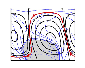
Since a thermal wave can have different modal shapes (see (3.2f)), here, we restrict our discussion for a uni-modal wave profile described by a single Fourier mode which reduces the lower wall thermal boundary condition to the following form:

(4.1)\begin{equation} \theta_L (x) = \tfrac{1}{2} Ra_{P,L} \cos (\alpha x). \end{equation}

Figure 2 illustrates the flow topologies and temperature fields in the slot. When the wave is stationary (i.e. wave phase speed $c=0$), the topology is elementary and exhibits symmetries – it consists of pairs of counter-rotating rolls with the wavelength dictated by the heating wavelength (figure 2a). The wave's movement breaks these symmetries. A slow wave travelling to the right separates the rolls from each other with a thin stream tube carrying fluid to the left (figure 2b). The anti-clockwise roll moves downwards and adheres to the lower wall. The clockwise roll moves upwards and adheres to the upper wall. The rolls now form separation bubbles. An increase of the wave speed to $c = 2$ (figure 2c) slightly reduces the size of the bubbles and increases the width of the stream tube, producing a larger net flow rate. The bubbles move down, becoming tilted to the left simultaneously. Further increase of the wave speed to $c = 10$ (figure 2d) continues the same process. Still further increase of the wave speed to $c = 20$ (figure 2e) shows the formation of a boundary layer near the heated wall with the majority of fluid not exposed to any heating.

Figure 2. Topology of flow (black) and temperature (blue) fields at (a) $c=0$, (b) $c=0.1$, (c) $c=2$, (d) $c=10$, (e) $c=20$ and ( f) $c=-2$ for $Ra_{p,L}=1000$, $\alpha =2$, $Pr=0.71$. The red colour shows the meandering flow stream. Shaded zones and dashed lines represent negative temperature.

The thermal wave is applied at the lower plate. As this wave diffuses into the fluid interior, it is delayed by the fluid thermal inertia, with its position falling further behind the surface wave as the distance from the lower plate increases. This process leads to bubble tilting. An increase in the wave velocity reduces the height to which the wave can diffuse, forming boundary layers.

The above process is symmetric to the wave direction, as a wave travelling to the left produces an equal but opposite response as a wave travelling to the right (compare figures 2(c) and 2( f)).

The separation bubbles act as rollers pulling the fluid along their edges. The lower bubble is exposed to a stronger convection, so its direction of rotation determines the direction of the net horizontal movement, which is opposite to the wave direction. This bubble rotates counterclockwise when the wave moves to the right, creating a net flow to the left (figure 2c), and rotates clockwise when the wave moves to the left, creating a net flow to the right (figure 2f). These rollers are the only source of propulsion responsible for the pumping effect. Figure 3(a,b) displays distributions of shear forces for different wave velocities. The shear distribution is symmetric when the wave is stationary and has zero mean value. Wave movement breaks this symmetry, producing a net shear force which initially increases with $c$, attains a maximum and begins to decrease with further increase of $c$ (figure 3c). Variations of the flow rate $Q$ induced by the net shear force as a function of the wave speed $c$ are shown in figure 4. The flow rate increases linearly with $c$, attains a maximum at $c = 2 \sim 3$ and then gradually decreases, eventually becoming proportional to $c^{-4}$.

Figure 3. Wall shear force $\tau _x$ distributions at the lower (a) and upper (b) plates for selected values of $c$ at $Ra_{p,L}=1000$, $\alpha =2$, $Pr=0.71$. Subscripts $L,U$ and $av$ denote lower, upper and average, respectively. Figure 3(c) displays the variation of the average shear stress as a function of the wave speed $c$. Asymptotes in this figure are shown by dashed lines.

Figure 4. Variation of the flow rate $Q$ as a function of the wave speed $c$ for selected values of $R_{p,L}$ at $\alpha =2$, $Pr=0.71$. Asymptotes are depicted by dashed lines.

In the following sections, we provide a detailed analysis of flow dynamics which provides further insight into the pumping mechanics.

4.1. Slow waves

In this section we describe system response to slow waves ($c \rightarrow 0$) and assume the flow quantities to be in the form of power series in terms of $c$, i.e.

(4.2)\begin{equation} [u,v,\theta,p]=[u_0, v_0,\theta_0, p_0]+ c [u_1, v_1,\theta_1, p_1] + O(c^2). \end{equation}

The flow rate can be represented in a similar manner as $Q = Q_0+c Q_1 +O(c^2)= \int _{-1} ^{+1} (u_0 + c u_1)\,{{\rm d}y} +O(c^2)$.

Substitution of the expansion (4.2) into (3.2) and extraction of the leading-order terms results in the following systems:

(4.3a)\begin{gather} O(1): u_0\frac{\partial u_0 }{\partial x} + v_0\frac{\partial u_0}{\partial y} ={-}\frac{\partial p_0}{\partial x}+ \frac{\partial ^2 u_0}{\partial x^2}+\frac{\partial ^2 u_0}{\partial y^2}, \end{gather}

(4.3b)\begin{gather}u_0\frac{\partial v_0 }{\partial x} + v_0\frac{\partial v_0}{\partial y} ={-}\frac{\partial p_0}{\partial y}+\frac{\partial ^2 v_0}{\partial x^2}+\frac{\partial ^2 v_0}{\partial y^2} + \frac{\theta_0}{Pr}, \end{gather}

(4.3c)\begin{gather}u_0\frac{\partial \theta_0 }{\partial x} + v_0\frac{\partial \theta_0}{\partial y} = \frac{1}{Pr} \left[\frac{\partial ^2 \theta_0}{\partial x^2}+\frac{\partial ^2 \theta_0}{\partial y^2} \right], \end{gather}

(4.3d)\begin{gather}\frac{\partial u_0 }{\partial x} + \frac{\partial v_0}{\partial y} = 0. \end{gather}

(4.4a)\begin{gather} O(c): u_0\frac{\partial u_1 }{\partial x} +u_1\frac{\partial u_0 }{\partial x}-\frac{\partial u_0 }{\partial x} + v_0\frac{\partial u_1}{\partial y} + v_1\frac{\partial u_0}{\partial y} ={-}\frac{\partial p_1}{\partial x}+\frac{\partial ^2 u_1}{\partial x^2}+\frac{\partial ^2 u_1}{\partial y^2}, \end{gather}

(4.4b)\begin{gather}u_0\frac{\partial v_1 }{\partial x} +u_1\frac{\partial v_0 }{\partial x}-\frac{\partial v_0 }{\partial x} + v_0\frac{\partial v_1}{\partial y} + v_1\frac{\partial v_0}{\partial y} ={-}\frac{\partial p_1}{\partial y}+\frac{\partial ^2 v_1}{\partial x^2}+\frac{\partial ^2 v_1}{\partial y^2}+ \frac{\theta_1}{Pr}, \end{gather}

(4.4c)\begin{gather}u_0\frac{\partial \theta_1 }{\partial x} +u_1\frac{\partial \theta_0 }{\partial x} -\frac{\partial \theta_0 }{\partial x}+ v_0\frac{\partial \theta_1}{\partial y} + v_1\frac{\partial \theta_0}{\partial y} = \frac{1}{Pr} \left[\frac{\partial ^2 \theta_1}{\partial x^2}+\frac{\partial ^2 \theta_1}{\partial y^2} \right], \end{gather}

(4.4d)\begin{gather}\frac{\partial u_1 }{\partial x} + \frac{\partial v_1}{\partial y} = 0. \end{gather}

One may note that the $O(1)$ system describes the natural convection due to spatial periodic heating with $c=0$. Such a flow system was analysed by Hossain & Floryan (Reference Hossain and Floryan2013) who represented the solution in the form

(4.5)\begin{equation} [u_0,v_0,\theta_0, p_0] = \sum_{n={-}\infty}^{n={+}\infty} [u_0^{(n)}, v_0^{(n)}, \theta_0^{(n)}, p_0^{(n)}] \exp({{\rm i} n \alpha x}), \end{equation}

and demonstrated that a horizontal flow rate was not possible since $u_0^{(0)} =0$ and $v_0 ^{(0)} =0$.

An aperiodic component of $u$-velocity $u_1^{(0)}$ exists in the $O(c)$ problem. We express $(u_1, v_1, \theta _1, p_1)$ in terms of Fourier expansions

(4.6)\begin{equation} [u_1,v_1,\theta_1, p_1] = \sum_{n={-}\infty}^{n={+}\infty} [u_1^{(n)}, v_1^{(n)}, \theta_1^{(n)}, p_1^{(n)}] \exp({{\rm i} n \alpha x}). \end{equation}

Substitution of the above expansions into (4.4a) yields

(4.7)\begin{align} & \sum_{m={-}\infty}^{m={+}\infty} [{\rm i} m \alpha u_0^{(n-m)} u_1^{(m) } + {\rm i} (n-m) \alpha u_0^{(n-m)} u_1^{(m)} + v_0^{(n-m)} Du_1^{(m)} + v_1^{(m)} Du_0^{(n-m)}] \nonumber\\ &\quad -{\rm i} n \alpha u_0^{(n)} ={-}{\rm i} n \alpha p_1^{(n)}-n^2 \alpha^2 u_1^{(n)}+ D^2 u_1^{(n)} . \end{align}

Extraction of mode 0 from (4.7) leads to

(4.8)\begin{equation} D^2 u_1^{(0)} = \sum_{m={-}\infty,\ m\!\neq 0}^{m={+}\infty} [v_0^{({-}m)} Du_1^{(m)} + v_1^{(m)} Du_0^{({-}m)}], \end{equation}

and its integration yields an aperiodic $u$-velocity $u_1^{(0)}$. The role of thermal waves is to set up a velocity field at $O(c)$ which produces Reynolds stresses at $O(c)$ (right-hand side of (4.8)) which drive the net horizontal flow.

Therefore, the net flow rate $Q= c \int u_1^{(0)}\,{{\rm d}y} + O(c^2)$, and the asymptote is depicted in figure 4.

4.2. Fast waves

The foregoing discussion elucidates that a high wave speed reduces the pumping effectiveness as the heat is carried away by the wave. Figure 5 demonstrates that velocity and temperature boundary layers are formed, and convective motions are concentrated very near to the lower wall. The formation of thin velocity and temperature boundary layers facilitates analysis in the limit $c \rightarrow \infty$. The temperature field is decomposed into two parts: one associated with the conduction state that occurs before the outset of the convection and is denoted as $\theta _0$, and the other associated with the convective modifications and is denoted as $\theta _1$ such that $\theta =\theta _0+\theta _1$. For the case of high velocity waves, i.e. $c \rightarrow \infty$, one can simplify the conduction solution to the following form:

(4.9)\begin{equation} \theta_0 = \frac{Ra_{p,L}}{4} \exp({-A(1+y)}) \exp({{\rm i} A(1+y)}) \exp({{\rm i} \alpha x})+c.c. \end{equation}

In the above, $A=\sqrt {\alpha c Pr /2}$, the term $\exp ({{\rm i} A(1+y)})$ provides a sinusoidal temperature variation with $y$, whereas the term $\exp ({-A(1+y)})$ shows an exponential decrease of temperature amplitude as $y$ increases. We introduce the stretched scale $\eta = \sqrt {c}(1 + y)$ in the vertical direction, and represent the inner solution as expansions of the form

(4.10a)$$\begin{gather} {[u_{inner},v_{inner},\theta_{inner}]=\sum_{n=2}^{8} c^{{-}n/2} [U_n(x,\eta),V_n(x,\eta),\varTheta_n(x,\eta)]+O(c^{{-}9/2})}, \end{gather}$$

(4.10b)$$\begin{gather}{[p_{inner}]=\sum_{n=1}^{7}c^{{-}n/2} P_n(x,\eta)+O(c^{{-}4}). } \end{gather}$$

Figure 5. (a) Temperature ($\theta /Ra_{p,L}$) and (b) $u$-velocity profiles for $c=3000$, $Ra_{p,L}=1000$, $\alpha =3$, $Pr=0.71$.

Substitution of (4.10) into the field equations (3.2) and separation of terms of equal orders of magnitude reveals that several leading-order equations provide trivial solutions. The equations that would provide non-zero solutions have the following form:

(4.11)\begin{equation} O(c^{{-}1}): \frac{\partial P_1}{\partial \eta} = \frac{\theta_0}{Pr}, \end{equation}

which describes a periodic pressure field $P_1$ created by the heating

(4.12)\begin{equation} O(c^{{-}3/2}): \frac{\partial ^2 U_3}{\partial \eta^2} +\frac{\partial U_3}{\partial x} = \frac{\partial P_1}{\partial x}, \end{equation}

which shows that $P_1$ produces a periodic horizontal velocity, $U_3$,

(4.13a,b)\begin{equation} O(c^{{-}2}): \frac{\partial U_3}{\partial x}+\frac{\partial V_4}{\partial \eta}=0,\quad \frac{\partial P_3}{\partial \eta}=\frac{\partial ^2 V_4}{\partial \eta^2} + \frac{\partial V_4}{\partial x}, \end{equation}

which shows that conservation of mass produces a periodic vertical velocity $V_4$ which, in turn, produces a periodic pressure $P_3$. Further analysis shows that

(4.14a,b)\begin{align} O(c^{{-}5/2}): \frac{\partial ^2 U_5}{\partial \eta^2} + \frac{\partial U_5}{\partial x}=\frac{\partial P_3}{\partial x} - \frac{\partial ^2 U_3}{\partial x^2},\quad \frac{\partial ^2 \varTheta_5}{\partial \eta^2} +Pr \frac{\partial \varTheta_5}{\partial x}=Pr U_3 \frac{\partial \theta_0}{\partial x} + Pr V_4 \frac{\partial \theta_0}{\partial \eta}, \end{align}

with the resulting $U_5$ being periodic but $\varTheta _5$ becoming aperiodic. In the next step

(4.15a,b)\begin{equation} O(c^{{-}3}): \frac{\partial U_5}{\partial x}+\frac{\partial V_6}{\partial \eta}=0, \quad \frac{\partial P_5}{\partial \eta}=\frac{\partial ^2 V_6}{\partial \eta^2} +\frac{\partial V_6}{\partial x}+ \frac{\partial ^2 V_4}{\partial x^2}, \end{equation}

which shows that conservation of mass produces a periodic velocity $V_6$ and interaction of $V_4$ and $V_6$ velocities yields the periodic pressure $P_5$. In the next step

(4.16)\begin{equation} O(c^{{-}7/2}): \frac{\partial ^2 U_7}{\partial \eta^2} + \frac{\partial U_7}{\partial x}= \frac{\partial P_5}{\partial x} - \frac{\partial ^2 U_5}{\partial x^2}, \end{equation}

where $U_5$ and $P_5$ generate the periodic velocity $U_7$ and, finally,

(4.17)\begin{equation} O(c^{{-}4}): \frac{\partial ^2 U_8}{\partial \eta^2} + \frac{\partial U_8}{\partial x}=\frac{\partial P_6}{\partial x} +U_3 \frac{\partial U_3}{\partial x}+V_4\frac{\partial U_3}{\partial \eta}, \end{equation}

generates an aperiodic velocity $U_8$. One may note that any constant involved in evaluating $U_8$ has to be determined by matching with the outer solution (see § 6.2). Evaluation of the flow rate yields

(4.18)\begin{equation} Q= c^{{-}4} \int_{{-}1}^1 U_8\,{{\rm d}y} + O(c^{{-}9/2}), \end{equation}

and is shown in figure 4.

5. Effect of heating intensity

Heating intensity enters the analysis in the form of the wave amplitude $Ra_{p,L}$. Figure 6(a) shows that the flow rate $Q$ increases proportionally to $Ra^2_{p,L}$ with the increase of $Ra_{p,L}$, but the nonlinear saturation limits this increase at high enough $Ra_{p,L}$. The saturation is also observed in the shear force (see figure 6b).

Figure 6. Variations of the flow rate $Q$ (a) and the average shear force $\tau _{av}$ (b) as functions of the heating intensity $Ra_{p,L}$ for $\alpha =2$, $Pr=0.71$.

5.1. Weak heating and mechanism of pumping

To demonstrate the mechanism of pumping activated by the thermal wave, we start with low intensity waves. We introduce a parameter $\epsilon$ as a measure of the heating intensity. We assume $\epsilon <<1$ and represent the flow variables in terms of asymptotic power series of $\epsilon$ as

(5.1)\begin{equation} (u,v,\theta,p)=\epsilon (U_1, V_1,\varTheta_1, P_1)+ \epsilon^2 [U_2, V_2,\varTheta_2, P_2] + O(\epsilon^3). \end{equation}

Substitution of (5.1) into (3.2) leads to a system of $O(\epsilon )$ in the form

(5.2a)$$\begin{gather} \frac{\partial ^2 U_1 }{\partial x^2} +\frac{\partial ^2 U_1 }{\partial y^2} +c \frac{\partial U_1 }{\partial x} -\frac{\partial P_1 }{\partial x} =0, \end{gather}$$

(5.2b)$$\begin{gather}\frac{\partial ^2 V_1 }{\partial x^2} +\frac{\partial ^2 V_1 }{\partial y^2}+c \frac{\partial V_1 }{\partial x} -\frac{\partial P_1 }{\partial y} = -Pr^{{-}1} \varTheta_1, \end{gather}$$

(5.2c)$$\begin{gather}\frac{\partial ^2 \varTheta_1 }{\partial x^2} +\frac{\partial ^2 \varTheta_1 }{\partial y^2} + c Pr \frac{\partial \varTheta_1 }{\partial x} =0 , \end{gather}$$

(5.2d)$$\begin{gather}\frac{\partial U_1 }{\partial x} + \frac{\partial V_1 }{\partial y} = 0, \end{gather}$$

(5.2e–h)$$\begin{gather}U_1(\pm1)=V_1(\pm1)=0,\quad \varTheta_L (x) = \frac{1}{2} Ra_{p,L} \cos(\alpha x), \quad \varTheta_U (x) =0,\quad \left.\frac{\partial P_1}{\partial x}\right|_{mean}= 0, \end{gather}$$

and a system of $O(\epsilon ^2)$ in the form

(5.3a)\begin{gather} \frac{\partial ^2 U_2 }{\partial x^2} +\frac{\partial ^2 U_2 }{\partial y^2} +c \frac{\partial U_2 }{\partial x} -\frac{\partial P_2 }{\partial x} = U_1 \frac{\partial U_1 }{\partial x} + V_1 \frac{\partial U_1 }{\partial y}, \end{gather}

(5.3b)\begin{gather}\frac{\partial ^2 V_2 }{\partial x^2} +\frac{\partial ^2 V_2 }{\partial y^2}+c \frac{\partial V_2 }{\partial x} -\frac{\partial P_2 }{\partial y} = -Pr^{{-}1} \varTheta_2 + U_1 \frac{\partial V_1 }{\partial x} + V_1 \frac{\partial V_1 }{\partial y}, \end{gather}

(5.3c)\begin{gather}\frac{\partial ^2 \varTheta_2 }{\partial x^2} +\frac{\partial ^2 \varTheta_2 }{\partial y^2} + c Pr \frac{\partial \varTheta_2 }{\partial x} = Pr U_1 \frac{\partial \varTheta_1 }{\partial x} + Pr V_1 \frac{\partial \varTheta_1 }{\partial y}, \end{gather}

(5.3d)\begin{gather}\frac{\partial U_2 }{\partial x} + \frac{\partial V_2 }{\partial y} = 0, \end{gather}

which is subject to homogeneous boundary conditions and a constraint associated with the zero-mean-pressure-gradient condition.

Inspection of (5.2f) leads to a temperature field in the form

(5.4)\begin{equation} \varTheta_1 (x,y)= \varTheta_1^{(1)} (y) \exp({{\rm i}\alpha x}) + c.c., \end{equation}

where c.c. stands for the complex conjugate, and an energy equation of the form

(5.5a)\begin{equation} D^2 \varTheta_1^{(1)} -(\alpha^2 - i \alpha c Pr) \varTheta_1^{(1)}=0, \end{equation}

whose solution is

(5.5b)\begin{equation} \varTheta_1^{(1)} = \frac{Ra_{p,L}}{8} \left[\frac {\cosh(\vartheta y)}{\cosh (\vartheta) } - \frac {\sinh(\vartheta y)}{\sinh (\vartheta) } \right] \exp({{\rm i} \alpha x}), \end{equation}

with $\vartheta =\sqrt (\alpha ^2-{\rm i} c \alpha Pr)$.

Equations (5.2a,b) are reduced to a single equation of the form

(5.6)\begin{equation} \nabla^4 \varPsi_1 + c \frac{\partial }{\partial x}(\nabla^2 \varPsi)=Pr^{{-}1} \frac{\partial \varTheta_1}{\partial x}, \end{equation}

where $\varPsi _1$ denotes the streamfunction. The character of the forcing on the right-hand of (5.6) suggests a solution in the form

(5.7)\begin{equation} \varPsi_1 (x,y)= \varPsi_1^{(1)} (y) \exp({{\rm i}\alpha x}) + c.c. \end{equation}

Substitution of (5.4) and (5.7) into (5.6) leads to

(5.8a)\begin{gather} D^4 \varPsi_1^{(1)} + ({\rm i} \alpha c -2 \alpha^2) D^2 \varPsi_1^{(1)} +(\alpha^4 -{\rm i} \alpha^3 c) \varPsi_1^{(1)} ={\rm i} \alpha Pr^{{-}1} \varTheta_1^{(1)}=F_1, \end{gather}

(5.8b)\begin{gather}\varPsi_1^{(1)}(\pm1)= D\varPsi_1^{(1)}(\pm1)=0, \end{gather}

where right-hand side $F_1$ represents the flow forcing (the $x$-component of the gradient of the buoyancy force). The velocity components have the form

(5.9a)\begin{gather} U_1= \frac{\partial \varPsi_1^{(1)}}{\partial y} = D \varPsi_1^{(1)}(y) \exp({{\rm i}\alpha x}) +c.c. = U_1^{(1)}(y) \exp({{\rm i}\alpha x}) +c.c., \end{gather}

(5.9b)\begin{gather}V_1={-} \frac{\partial \varPsi_1^{(1)}}{\partial x} ={-}{\rm i} \alpha \varPsi_1^{(1)}(y) \exp({{\rm i}\alpha x}) +c.c. = V_1^{(1)}(y) \exp({{\rm i}\alpha x}) +c.c.\end{gather}

Analysis of $O(\epsilon ^2)$ equations shows that the unknowns can be represented as

(5.10a–c)\begin{align} [\varTheta_2,U_2,V_2 ](x,y)= [\varTheta_2^{(0)},U_2^{(0)},V_2^{(0)}] (y) + [\varTheta_2^{(2)},U_2^{(2)},V_2^{(2)}] (y)\exp({{\rm i}2\alpha x}) + c.c. \end{align}

It can easily be shown that $V_2^{(0)}=0$. Substitution of (5.9) and (5.10b,c) into (5.3a) and extraction of the zero modal function combined with the enforcement of the mean-pressure-gradient constraint lead to the following flow problem:

(5.11a–c)\begin{equation} D^2 U_2^{(0)} = g_1(y),\quad U_2^{(0)}({\pm} 1)=0,\quad g_1(y)=V_1^{({-}1)} DU_1^{(1)} + V_1^{(1)} DU_1^{({-}1)}. \end{equation}

Integration of (5.11a–c) gives $U_2^{(0)}$ whose integration gives the net flow $Q$, i.e.

(5.12a)\begin{equation} Q=\int_{{-}1}^{1} U_2^{(0)} \,{{\rm d}y} = K_1 -K_2, \end{equation}

where

(5.12b–d)\begin{equation} K_1=\int_{{-}1}^{1}\int_{{-}1}^{\eta} g(\eta)\,{\rm d}\eta\,{{\rm d}y},\quad K_2=\int_{{-}1}^{1} g(y)\,{{\rm d}y},\quad g(y)=\int g_1(y)\,{{\rm d}y}. \end{equation}

Equation (5.12) demonstrates that $g(y)$ (Reynolds stress) is responsible for the pumping effect. Equations (5.8) and (5.11a–c) have been solved numerically using the same collocation method as described in § 3, and integrations in (5.12) have been performed with fourth-order accuracy.

Figure 7 displays the real and imaginary parts of $\varTheta _1^{(1)}$ and its phase shift $\varPhi$ with respect to the wave imposed at the lower plate. As heat diffuses into the fluid interior, the thermal inertia delays the wave at each $y$-elevation with respect to the wave at the lower plate – the phase shift $\varPhi$ measures this delay. The modal function is purely real when the wave is stationary and the phase shift $\varPhi =0$. When the wave begins to move, the modal function becomes complex, and its imaginary part represents the wave-induced correction. The resulting phase shift illustrated in figure 7(c) shows that the delay increases as $c$ increases. At high wave speeds, the wave amplitude outside the boundary layer decreases with $y$ in an oscillatory manner, so one should look only at variations of $\varPhi$ within the boundary layer. The forcing function $F_1$ in (5.8) changes from purely imaginary when $c=0$ to being complex when $c\!\neq 0$ – its distribution is shown in figure 8(a), and the real part acts in the opposite direction to the wave motion. The Reynolds stress is zero when $c=0$ due to the orthogonality of the velocity components but becomes non-zero when $c\!\neq 0$ as shown in figure 8(b). The Reynolds stress acts in the direction opposite to the wave motion. Figure 9 explicitly illustrates the role of the wave-induced correction. The flow pattern obtained by using only the imaginary part of $F_1$ when solving (3.5a,b) is displayed in figure 9(a), when using only the real part of $F_1$ is displayed in figure 9(b), and when using the complete $F_1$ is displayed in figure 9(c). The imaginary part of $F_1$ creates regular rolls, and the real part creates stream tube.

Figure 7. Distributions of the real $\varTheta _r^{(1)}$ (a) and the imaginary $\varTheta _i^{(1)}$ (b) parts of the temperature modal function $\varTheta _1^{(1)}$, and the phase shift $\varPhi$ of $\varTheta _1^{(1)}$ with respect to the wave at the lower plate (c).

Figure 8. Distributions of the real part of the function $F_1$ (a), and the Reynolds stress $g(y)$ (b) for $\alpha =2$, $Ra_{p,L}=200$, $Pr=0.71$.

Figure 9. Flow topologies determined with (a) only imaginary part of forcing $F_1$ (b) only real part of forcing $F_1$ and (c) complete forcing $F_1$.

It can be concluded that the delay associated with the penetration of thermal waves into the fluid interior causes a change in the flow field, which generates Reynolds stress which drives the net fluid movement in the horizontal direction.

Having insight about the mechanism of the pumping action, we next focus our attention on the effect of wavelength.

6. Effect of wavelength

In this section we shall discuss the effect of the wavelength of the wave on the flow rate. We start with the long-wavelength heating as such a heating can be solved analytically, thus, providing explicit relations illustrating the underlying flow dynamics.

6.1. Long-wavelength waves

Let us consider long-wavelength waves which corresponds to the limit $\alpha \rightarrow 0$. We introduce a slow scale $\xi = \alpha x$, and represent the unknowns as power series in terms of $\alpha$ in the following form:

(6.1a)$$\begin{gather} [u(\xi,y),v(\xi,y),\theta(\xi,y)]=\sum_{n=1}^{4} \alpha^n [U_n (\xi,y),V_n (\xi,y),\varTheta_n(\xi,y)]+O(\alpha^5), \end{gather}$$

(6.1b)$$\begin{gather}p(\xi,y)=\sum_{n=0}^{3} \alpha^n P_n (\xi,y)+O(\alpha^4). \end{gather}$$

Substitution of (6.1) into the field equations (3.2) and extraction of the leading-order terms results in the following system:

(6.2a–d)\begin{gather} \frac{\partial ^2 \varTheta_0}{\partial y^2}=0,\ \ \frac{\partial P_0}{\partial y}=\frac{\varTheta_0}{Pr},\ \ \frac{\partial ^2 U_1}{\partial y^2}=\frac{\partial P_0}{\partial \xi},\ \ \frac{\partial V_1}{\partial y}=0, \end{gather}

(6.2e–h)\begin{gather}\varTheta_0({-}1)=(1/2)Ra_{p,L}\cos(\alpha x),\ \ \varTheta_0(1)=0,\ \ U_1({\pm} 1)=V_1({\pm} 1)=0,\ \ \left.\frac{\partial P_0}{\partial \xi} \right|_{mean}= 0. \end{gather}

Its solution is given as

(6.3a–c)\begin{align} \varTheta_0=\frac{Ra_{p,L}}{4}(1-y)\cos \xi,\quad U_1=\frac{Ra_{p,L}}{480Pr}(1-y^2)(1+20y-5y^2) \sin\xi,\quad V_1=0. \end{align}

The temperature changes linearly in $y$ and sinusoidally in $\xi$, and the velocity $U_1$ varies periodically in $\xi$.

The next order of the system

(6.4a–d)$$\begin{gather} \frac{\partial ^2 \varTheta_1}{\partial y^2}={-}cPr\frac{\partial \varTheta_0}{\partial \xi},\quad \frac{\partial P_1}{\partial y}=\frac{\varTheta_1}{Pr}, \quad \frac{\partial ^2 U_2}{\partial y^2}=\frac{\partial P_1}{\partial \xi}-c\frac{\partial U_1}{\partial \xi}, \quad \frac{\partial U_1}{\partial \xi} +\frac{\partial V_2}{\partial y}=0, \end{gather}$$

(6.4e–g)$$\begin{gather}\varTheta_1({\pm} 1)=0,\quad U_2({\pm} 1)=V_2({\pm} 1)=0,\quad \left.\frac{\partial P_1}{\partial \xi} \right|_{mean}= 0, \end{gather}$$

has the following solution:

(6.5a–c) \begin{align} \left.\begin{gathered} \varTheta_1={-}\frac{c Pr Ra_{p,L}}{24}H_{\varTheta,11} (y) \sin \xi,\quad U_2={-}\frac{c Ra_{p,L}}{100800Pr}[ H_{U,21} (y) +PrH_{U,22} (y)]\cos \xi,\\ V_2=-\frac{Ra_{p,L}}{480Pr} H_{V,21} (y)\cos \xi, \end{gathered}\right\} \end{align}

with coefficients $H_{\varTheta,11}$, $H_{U,21}$, $H_{U,22}$ and $H_{V,21}$ given in Appendix A. At this level of approximation, the wave generates a temperature correction which is able to create both horizontal and vertical fluid motions but these motions are unable to produce any net flow rate.

The next order of the system

(6.6a,b)$$\begin{gather} \frac{\partial ^2 \varTheta_2}{\partial y^2}={-}cPr\frac{\partial \varTheta_1}{\partial \xi} + Pr U_1 \frac{\partial \varTheta_0}{\partial \xi} + Pr V_2 \frac{\partial \varTheta_0}{\partial y}- \frac{\partial ^2 \varTheta_0}{\partial y^2}, \quad \frac{\partial P_2}{\partial y}=\frac{\partial ^2 V_2}{\partial y^2}+ \frac{\varTheta_2}{Pr}, \end{gather}$$

(6.6c,d)$$\begin{gather}\frac{\partial ^2 U_3}{\partial y^2}=\frac{\partial P_2}{\partial \xi}-c\frac{\partial U_2}{\partial \xi}-\frac{\partial ^2 U_1}{\partial \xi^2}+U_1 \frac{\partial U_1}{\partial \xi} +V_2 \frac{\partial U_1}{\partial y}, \quad \frac{\partial U_2}{\partial \xi} +\frac{\partial V_3}{\partial y}=0, \end{gather}$$

(6.6e–g)$$\begin{gather}\varTheta_2({\pm} 1)=0,\quad U_3({\pm} 1)=V_3({\pm} 1)=0,\quad \left.\frac{\partial P_2}{\partial \xi}\right|_{mean}= 0, \end{gather}$$

has solution of the form

(6.7) \begin{align} \left.\begin{aligned} \varTheta_2&=Ra_{p,L}^2 H_{\varTheta,20} (y) + Ra_{p,L} [H_{\varTheta,21} (y) +c^2 Pr^2 H_{\varTheta,22} (y)] \cos \xi \\ &\quad+ Ra_{p,L}^2 H_{\varTheta,23} (y) \cos(2 \xi),\\ U_3&= Ra_{p,L} \left[ c^2 [Pr H_{U,31} (y)+H_{U,32}(y)] + \frac{1}{Pr}[H_{U,33} (y)+ c^2 H_{U,34}(y)] \right] \sin \xi\\ &\quad +\frac{Ra_{p,L}^2}{Pr^2} [PrH_{U,35} (y)+H_{U,36} (y) ] \sin(2 \xi)\\ & V_3={-}\frac{c Ra_{p,L}}{100800Pr}[H_{V,31} (y) +Pr H_{V,32}] \sin \xi, \end{aligned}\right\} \end{align}

with coefficients $H_{\varTheta,20-23}$, $H_{U,31-36}$ and $H_{V,31-32}$ given in Appendix A. The temperature field has an aperiodic part (first term of the $\varTheta _2$ solution), but the velocity fields are still purely periodic. Hence we look for the next order of the system

(6.8a)$$\begin{gather} \frac{\partial ^2 \varTheta_3}{\partial y^2}={-}cPr\frac{\partial \varTheta_2}{\partial \xi} + Pr U_1 \frac{\partial \varTheta_1}{\partial \xi}+ Pr U_2 \frac{\partial \varTheta_0}{\partial \xi} + Pr V_2 \frac{\partial \varTheta_1}{\partial y}+ Pr V_3 \frac{\partial \varTheta_0}{\partial y}-\frac{\partial ^2 \varTheta_1}{\partial y^2}, \end{gather}$$

(6.8b)$$\begin{gather}\frac{\partial P_3}{\partial y}=c \frac{\partial V_2}{\partial \xi}+\frac{\partial ^2 V_3}{\partial y^2}+\frac{\varTheta_3}{Pr}, \end{gather}$$

(6.8c,d)\begin{gather} \left.\begin{gathered} \frac{\partial ^2 U_4}{\partial y^2} = \frac{\partial P_3}{\partial \xi}-c\frac{\partial U_3}{\partial \xi}-\frac{\partial ^2 U_2}{\partial \xi^2}+U_1 \frac{\partial U_2}{\partial \xi}+U_2 \frac{\partial U_1}{\partial \xi} +V_2 \frac{\partial U_2}{\partial y}+V_3 \frac{\partial U_1}{\partial y},\\ \frac{\partial U_3}{\partial \xi} +\frac{\partial V_4}{\partial y}=0, \end{gathered}\right\} \end{gather}

(6.8e–g)\begin{gather} \varTheta_3({\pm} 1)=0,\quad U_4({\pm} 1)=V_4({\pm} 1)=0,\quad \left.\frac{\partial P_3}{\partial \xi}\right|_{mean}= 0. \end{gather}

Close inspection of this system reveals that the first two equations provide periodic solutions, but the last four terms (denoted as $F(y)$ ) of the third equation provide an aperiodic forcing which is capable of producing an aperiodic solution $U_{4,aper}$ which generates a horizontal net flow.

The aperiodic part of $U_4$ can be expressed as

(6.9a)\begin{equation} U_4|_{aper}= \int_{{-}1}^{y} \int_{{-}1}^{\mu} F(\eta) \,{\rm d}\eta \,{\rm d}\mu -\frac{y+1}{2} \int_{{-}1}^{1} \int_{{-}1}^{\mu} F(\eta) \,{\rm d}\eta \,{\rm d}\mu, \end{equation}

and reduced after integration to

(6.9b)\begin{equation} U_4|_{aper}={-}\frac{c Ra_{p,L}^2}{12192768000 Pr^2} [H_{U,400}(y) + Pr H_{U,401}(y)], \end{equation}

giving the flow rate

(6.10)\begin{equation} Q_{aper} = \int_{{-}1}^{1} U_4|_{aper} \,{{\rm d}y} ={-}\frac{229 c Ra_{p,L}^2\alpha^4 (1+Pr)}{851350500 Pr^2}. \end{equation}

Coefficients $H_{U,400-401}$ are given in Appendix A. The flow rate is directed opposite to the wave direction and is proportional to ${\sim }\alpha ^4$. The net shear force exerted by the rollers (the upper and the lower bubbles) can be calculated as

(6.11)\begin{equation} \tau_{L,net} ={-}\frac{c Ra_{p,L}^2\alpha^4 (3+17Pr)}{11907000 Pr^2}={-}\tau_{U,net}. \end{equation}

Next, we focus our attention to the short-wavelength heating, as again, this case can be solved analytically.

6.2. Short-wavelength waves

We consider short-wavelength waves that corresponds to $\alpha \rightarrow \infty$, and in this limit, the conduction temperature field subject to (4.1) is approximated as

(6.12)\begin{equation} \theta_0 = \frac{Ra_{p,L}}{2} \exp({-\alpha (1+y)}) \cos(\alpha x), \end{equation}

demonstrating formation of a thin boundary layer close to the lower plate. We introduce a fast scale $\xi =\alpha x$ in the horizontal direction and a stretched scale $\varOmega = \alpha (1+y)$ along the vertical direction and express the solution in the inner layer in expansions in terms of $\alpha ^{-1}$ as

(6.13a)$$\begin{gather} [u_{in},v_{in},\theta_{in}]=\sum_{n=1}^{6}\alpha^{{-}n} [U_n(\xi,\varOmega),V_n(\xi,\varOmega),\varTheta_n(\xi,\varOmega)]+O(\alpha^{{-}7}), \end{gather}$$

(6.13b)$$\begin{gather}[p_{in}]=\sum_{n=0}^{5} \alpha^{{-}n} [P_n(\xi,\varOmega)]+O(\alpha^{{-}6}). \end{gather}$$

Substitution of (6.13) into (3.2) and retention of the leading-order terms result in the following $O(\alpha ^{-1} )$ system:

(6.14a,b)$$\begin{gather} \frac{\partial ^2 U_1}{\partial \xi^2}+\frac{\partial ^2 U_1}{\partial \varOmega^2} -\frac{\partial P_0}{\partial \xi}=0, \quad \frac{\partial ^2 V_1}{\partial \xi^2}+\frac{\partial ^2 V_1}{\partial \varOmega^2} -\frac{\partial P_0}{\partial \varOmega}=0, \end{gather}$$

(6.14c)$$\begin{gather}\frac{\partial ^2 \varTheta_1}{\partial \xi^2}+\frac{\partial ^2 \varTheta_1}{\partial \varOmega^2} = cPr \frac{Ra_{p,L}}{2} {\rm e}^{-\varOmega} \sin \xi, \end{gather}$$

(6.14d–f)$$\begin{gather}U_1({\pm} 1)=V_1({\pm} 1)=0,\quad \varTheta_1({\pm} 1)=0,\quad \left.\frac{\partial P_0}{\partial \xi}\right|_{mean}= 0. \end{gather}$$

Elimination of the pressure from (6.14a,b) and introduction of the streamfunction lead to a system of partial differential equations for streamfunction and temperature. Their solution, which can be determined using method of separation of variables, has the form

(6.14g–i)\begin{equation} U_1=0, \quad V_1=0, \quad \varTheta_1={-}\tfrac{1}{4}c Pr Ra_{p,L} \varOmega \,{\rm e}^{-\varOmega} \sin\xi. \end{equation}

One can observe that the temperature field is affected by the wave but without creating any convection. System $O(\alpha ^{-2} )$ has the following form:

(6.15a,b)$$\begin{gather} \frac{\partial ^2 U_2}{\partial \xi^2}+\frac{\partial ^2 U_2}{\partial \varOmega^2} -\frac{\partial P_1}{\partial \xi}=0,\quad \frac{\partial ^2 V_2}{\partial \xi^2}+\frac{\partial ^2 V_2}{\partial \varOmega^2} -\frac{\partial P_1}{\partial \varOmega}={-}\frac{Ra_{p,L}}{2Pr} {\rm e}^{-\varOmega} \cos\xi, \end{gather}$$

(6.15c)$$\begin{gather}\frac{\partial ^2 \varTheta_2}{\partial \xi^2}+\frac{\partial ^2 \varTheta_2}{\partial \varOmega^2} ={-}cPr \frac{\partial \varTheta_1}{\partial \xi}, \end{gather}$$

(6.15d–f)$$\begin{gather}U_2({\pm} 1)=V_2({\pm} 1)=0,\quad \varTheta_2({\pm} 1)=0,\quad \left.\frac{\partial P_1}{\partial \xi}\right|_{mean}= 0, \end{gather}$$

and its solution can be written as

(6.15g,h)$$\begin{gather} U_2=\frac{Ra_{p,L}}{16Pr} \varOmega ({-}2+\varOmega) \,{\rm e}^{-\varOmega} \sin\xi,\quad V_2=\frac{Ra_{p,L}}{16Pr} \varOmega^2 \,{\rm e}^{-\varOmega} \cos\xi, \end{gather}$$

(6.15i)$$\begin{gather}\varTheta_2={-}\frac{1}{16}c^2 Pr^2 Ra_{p,L} \varOmega (1+\varOmega) \,{\rm e}^{-\varOmega} \cos\xi. \end{gather}$$

At this level of approximation, the heating creates periodic motion. System $O(\alpha ^{-3})$ has the following form:

(6.16a,b)$$\begin{gather} \frac{\partial ^2 U_3}{\partial \xi^2}+\frac{\partial ^2 U_3}{\partial \varOmega^2} -\frac{\partial P_2}{\partial \xi}={-}c\frac{\partial U_2}{\partial \xi}, \quad \frac{\partial ^2 V_3}{\partial \xi^2}+\frac{\partial ^2 V_3}{\partial \varOmega^2} -\frac{\partial P_2}{\partial \varOmega}={-}c\frac{\partial V_2}{\partial \xi}-\frac{\varTheta_1}{Pr}, \end{gather}$$

(6.16c)$$\begin{gather}\frac{\partial ^2 \varTheta_3}{\partial \xi^2}+\frac{\partial ^3 \varTheta_3}{\partial \varOmega^2} ={-}cPr \frac{\partial \varTheta_2}{\partial \xi} - \frac{Pr Ra_{p,L}}{2} {\rm e}^{-\varOmega} [U_2 \sin\xi +V_2 \cos\xi], \end{gather}$$

(6.16d–f)$$\begin{gather}U_3({\pm} 1)=V_3({\pm} 1)=0,\quad \varTheta_3({\pm} 1)=0,\quad \left.\frac{\partial P_2}{\partial \xi} \right|_{mean}= 0, \end{gather}$$

and its solution can be written as

(6.16g)$$\begin{gather} U_3=\frac{c Ra_{p,L}}{192Pr} [{-}6-3\varOmega+2\varOmega^2+2Pr({-}6+\varOmega^2)] \,{\rm e}^{-\varOmega} \cos\xi, \end{gather}$$

(6.16h)$$\begin{gather}V_3={-}\frac{cRa_{p,L}}{192Pr} \varOmega^2 [3+2\varOmega+2Pr(3+\varOmega)] \,{\rm e}^{-\varOmega} \sin\xi, \end{gather}$$

(6.16i)\begin{gather} \varTheta_3 = \frac{1}{256} [Ra_{p,L}^2 +256 B_2\varOmega -{\rm e}^{{-}2\varOmega} Ra_{p,L}^2 (1+2\varOmega+2\varOmega^2) ] \nonumber\\ -\,\frac{c^3 Pr^3 Ra_{p,L}}{96}\varOmega(3+3\varOmega+\varOmega^2) \,{\rm e}^{-\varOmega}\cos\xi \nonumber\\ +\,\frac{Ra_{p,L}}{512}{\rm e}^{{-}2\varOmega} \varOmega (1+2\varOmega) \cos(2\xi). \end{gather}

The velocity field remains periodic, whereas the temperature field produces a net heat transfer between the plates described by the first bracketed term in $\varTheta _3$ and the constant $B_2$ in this term is to be calculated from the matching with the outer solution. The system $O(\alpha ^{-4})$ has the following form:

(6.17a,b)\begin{gather} \frac{\partial ^2 U_4}{\partial \xi^2}+\frac{\partial ^2 U_4}{\partial \varOmega^2} -\frac{\partial P_3}{\partial \xi}={-}c\frac{\partial U_3}{\partial \xi}, \quad \frac{\partial ^2 V_4}{\partial \xi^2}+\frac{\partial ^2 V_4}{\partial \varOmega^2} -\frac{\partial P_3}{\partial \varOmega}={-}c\frac{\partial V_3}{\partial \xi}-\frac{\varTheta_2}{Pr}, \end{gather}

(6.17c)\begin{gather} \frac{\partial ^2 \varTheta_4}{\partial \xi^2}+\frac{\partial ^3 \varTheta_4}{\partial \varOmega^2} ={-}cPr \frac{\partial \varTheta_3}{\partial \xi} - \frac{Pr Ra_{p,L}}{2} {\rm e}^{-\varOmega} [U_3 \sin\xi +V_3 \cos\xi] \nonumber\\ \qquad +\,Pr\left[U_2 \frac{\partial \varTheta_1}{\partial \xi}+V_2 \frac{\partial \varTheta_1}{\partial \varOmega}\right], \end{gather}

(6.17d–f)\begin{gather} U_4({\pm} 1)=V_4({\pm} 1)=0,\quad \varTheta_4({\pm} 1)=0,\quad \left.\frac{\partial P_3}{\partial \xi}\right|_{mean}= 0, \end{gather}

whose solution can be written as

(6.17g)\begin{gather} U_4 ={-}\frac{ c^2 Ra_{p,L}\,{\rm e}^{-\varOmega}}{768Pr}[{-}12-6\varOmega+\varOmega^3+ Pr({-}18-9\varOmega+2\varOmega^2+\varOmega^3) \nonumber\\ +\,Pr^2({-}30-3\varOmega+2\varOmega^2+\varOmega^3)]\sin\xi, \end{gather}

(6.17h)\begin{gather} V_4={-}\frac{c^2 Ra_{p,L}\,{\rm e}^{-\varOmega}}{768Pr} \varOmega^2 [6+4\varOmega+\varOmega^2+Pr(3+\varOmega)^2+Pr^2(15+6\varOmega+\varOmega^2)] \cos\xi, \end{gather}

(6.17i)\begin{gather} \varTheta_4 = \frac{c^4 Pr^4 Ra_{p,L} \,{\rm e}^{-\varOmega}}{768} \varOmega (15+15\varOmega+6 \varOmega^2 + \varOmega^3 ) \sin \xi \nonumber\\ - \,\frac{c Ra_{p,L}^2 \,{\rm e}^{{-}2\varOmega}}{12\,288} \varOmega (9+18 \varOmega + 8 \varOmega^2 + 24 Pr (1+\varOmega)^2) \sin(2 \xi). \end{gather}

The velocity field is still periodic, so we look into the $O(\alpha ^{-5})$ system which has the following form:

(6.18a)$$\begin{gather} \frac{\partial ^2 U_5}{\partial \xi^2}+\frac{\partial ^2 U_5}{\partial \varOmega^2} -\frac{\partial P_4}{\partial \xi}={-}c\frac{\partial U_4}{\partial \xi}+U_2 \frac{\partial U_2}{\partial \xi} +V_2 \frac{\partial U_2}{\partial \varOmega}, \end{gather}$$

(6.18b)$$\begin{gather}\frac{\partial ^2 V_5}{\partial \xi^2}+\frac{\partial ^2 V_5}{\partial \varOmega^2} -\frac{\partial P_4}{\partial \varOmega}={-}c\frac{\partial V_4}{\partial \xi}+U_2 \frac{\partial V_2}{\partial \xi}+V_2 \frac{\partial V_2}{\partial \varOmega}-\frac{\varTheta_3}{Pr}, \end{gather}$$

(6.18c)\begin{gather} \frac{\partial ^2 \varTheta_5}{\partial\xi^2}+\frac{\partial ^2 \varTheta_5}{\partial \varOmega^2}={-}cPr \frac{\partial \varTheta_4}{\partial \xi} - \frac{Pr Ra_{p,L}}{2} {\rm e}^{-\varOmega} [U_4 \sin\xi +V_4 \cos\xi] \nonumber\\ \hspace{9.5pc} +\,Pr\left[U_2 \frac{\partial \varTheta_2}{\partial \xi}+U_3 \frac{\partial \varTheta_1}{\partial \xi}+V_2 \frac{\partial \varTheta_2}{\partial \varOmega}+V_3 \frac{\partial \varTheta_1}{\partial \varOmega}\right], \end{gather}

(6.18d–f)\begin{gather} U_5({\pm} 1)=V_5({\pm} 1)=0,\quad \varTheta_5({\pm} 1)=0,\quad \left.\frac{\partial P_4}{\partial \xi}\right|_{mean}= 0. \end{gather}

The above system still provides only a periodic velocity field. Hence it is necessary to analyse the $\xi$-momentum equation in $O(\alpha ^{-6})$ system, i.e.

(6.19a)$$\begin{gather} \frac{\partial ^2 U_6}{\partial \xi^2}+\frac{\partial ^2 U_6}{\partial \varOmega^2} -\frac{\partial P_5}{\partial \xi}={-}c\frac{\partial U_5}{\partial \xi}+U_2 \frac{\partial U_3}{\partial \xi}+U_3 \frac{\partial U_2}{\partial \xi} +V_2 \frac{\partial U_3}{\partial \varOmega}+V_3 \frac{\partial U_2}{\partial \varOmega}. \end{gather}$$

(6.19b)$$\begin{gather}U_6({\pm} 1)=V_6({\pm} 1)=0,\quad \left.\frac{\partial P_5}{\partial \xi} \right|_{mean}= 0. \end{gather}$$

The last four terms of the right-hand side of (6.19a) are aperiodic, and the aperiodic part of the solution $U_{6,aper}$ can easily be determined as

(6.20)\begin{equation} U_{{6,aper}} =B_3 \varOmega -\frac{cRa_{p,L}^2 (1+Pr)}{4096 Pr^2} \left[1-\frac{1}{3}(3+6\varOmega+6\varOmega^2+4\varOmega^3+2\varOmega^4)\right]. \end{equation}

The constant $B_3$ needs to be determined by matching with the outer solution.

One can note that the outer solution cannot be a function of $x$ as all $x$-variations are confined to the boundary layer. Consequently, we assume the outer solution to be of the following form:

(6.21a,b)$$\begin{gather} u_{outer} (x,y)= \alpha^{{-}6} \widehat{U}_6 + O(\alpha^{{-}7}),\quad v_{outer} (x,y)=0, \end{gather}$$

(6.21c,d)$$\begin{gather}p_{outer} (x,y)= \alpha^{{-}3} \widehat{P}_3 + O(\alpha^{{-}4}), \quad \theta_{outer} (x,y)= \alpha^{{-}3} \widehat{\varTheta}_3 + O(\alpha^{{-}4}). \end{gather}$$

Substitution of (6.21) into the field equations and retention of the leading-order terms result in the following system:

(6.22a–c)\begin{equation} \frac{\partial ^2 \widehat{U_6}}{\partial y^2} =0, \quad \frac{\partial \widehat{P_3}}{\partial y} = \frac{\widehat{\varTheta_3}}{Pr}, \quad \frac{\partial ^2 \widehat{\varTheta_3}}{\partial y^2} =0, \end{equation}

whose solutions have the form

(6.22d–f)\begin{equation} \widehat{U_6}(y) =\widehat{A_6}(y-1), \quad \widehat{P_3}(y) =\widehat{A_3}(y^2/2-y), \quad \widehat{\varTheta_3}(y) =\widehat{A_3} (y-1). \end{equation}

Constants $\widehat {A_3}$ and $\widehat {A_6}$ are determined from the matching with the inner solution, and the matching process provides

(6.23)\begin{equation} U_{{6,aper}} ={-}\frac{cRa_{p,L}^2 (1+Pr)}{4096 Pr^2} \left[(1-y)-\frac{1}{3}(3+6\varOmega+6\varOmega^2+4\varOmega^3+2\varOmega^4)\right]. \end{equation}

Therefore, the net flow

(6.24)\begin{equation} Q ={-}\frac{cRa_{p,L}^2 (1+Pr)}{4096 Pr^2} \alpha^{{-}6} + O(\alpha^{{-}7}). \end{equation}

As $\alpha \rightarrow \infty$, the flow rate Q decreases proportionally to ${\sim }\alpha ^{-6}$ and the proper asymptote is depicted in figure 10.

Figure 10. Variations of the flow rate $Q$ as a function of the heating wavenumber $\alpha$ for $Ra_{p,L}=1000$, $Pr=0.71$. Asymptotes are depicted by dashed lines.

6.3. Waves with moderate wavelength

Having observed the flow structures at small and large $\alpha$ values, we now investigate the in between $\alpha$ values . Figure 10 shows that the mean flow rate increases with the increase of $\alpha$, attains a maximum value at $\alpha = 2.2$, 2 and 1.3 for $c= 0.1$, 2 and 10, respectively. There is a specific $\alpha$ for each wave speed $c$ which provides the maximum flow rate, and this $\alpha$ does not vary too much $(\alpha = 1.3 \sim 2.2)$ with the increase of $c$ for $c=0.1 \sim 10$. Figure 11 illustrates the variations of the flow rate $Q$ as function of the wavenumber $\alpha$ and the wave speed $c$. Large $\alpha$ ($\alpha >7$) and large wave speed $c$ ($c>10$) provide $Q \sim O(10^{-2})$ and lower. It is found that $1<\alpha <4$ and $c = 1 \sim 5$ are most effective in generating large $Q (>0.5)$.

Figure 11. Variations of the flow rate $Q$ as a function of the wavenumber $\alpha$ and the wave speed $c$ for $Ra_{p,L} =1000$, $Pr$=0.71.

7. Effect of Prandtl number

The role of the Prandtl number $Pr$ in the induced flow rate $Q$ is explicitly illustrated in figure 12. Variations of the flow rate with $c$ are qualitatively similar for all types of fluids considered (figure 12a). Variation of the flow rate with $\alpha$ also follows a similar course for all types of fluids considered (figure 12b). The flow rate decreases with the increase of $Pr$ (figure 12c). The low-$Pr$ fluids generate higher $Q$ than the high-$Pr$ fluids as the thermal wave diffuses quickly into the fluid interior, causing a more intense fluid movement whereas, for high-$Pr$ fluids, the wave diffuses slowly. It is found numerically that the flow rate varies proportional to ${\sim }Pr^{-5}$ for high-$Pr$ fluids.

Figure 12. Variations of the flow rate $Q$ as a function of (a) wave speed $c$ at $\alpha =2$, (b) wavenumber $\alpha$ at $c=2$, (c) Prandtl number $Pr$ at $\alpha =2$, $c=2$ for $Ra_{p,L}=500$. In (c), the asymptote is depicted by dashed line.

8. Waves at the upper plate

We discuss how the flow response is changed when the thermal waves are moved to the upper plate. The resulting thermal boundary conditions take the following form:

(8.1a,b)\begin{equation} \theta_L (x) = 0,\quad \theta_U (x) =\tfrac{1}{2} Ra_{P,U} \cos (\alpha x). \end{equation}

One can easily find a correlation between the fluid response to waves at the lower and upper plates. If we set up a problem considering the thermal wave on the lower plate with $Ra_{P,L}=A$ and $Ra_{P,U}=0$ and take the transformation $Ra_{P,L} \rightarrow 0$, $Ra_{P,U} \rightarrow A$, $u \rightarrow -U$, $v \rightarrow -V$, $p \rightarrow P$, $\theta \rightarrow -\varTheta$, $x \rightarrow -X+{\rm \pi}$, $y \rightarrow -Y$, together with the thermal boundary conditions reversed in sign, the resulting governing equations become identical. Consequently, all the properties of the flow system with a thermal wave applied on the upper plate can be deduced directly from the analysis of the system with a wave on the lower plate.

9. Summary

Effects of thermal waves propagating along the boundary of a horizontal conduit were investigated. The investigation considered sinusoidal waves propagating either along the lower or the upper plate. The wave was characterized by the wave speed $c$, the wavenumber $\alpha$ and the amplitude expressed in terms of a Rayleigh number $Ra_{p,L}$. The flow problem was solved with spectral accuracy in the reference frame moving with the wave speed using Fourier expansions in the horizontal direction and the collocation method in the vertical direction. Analytic solutions were determined for the large and small wavenumber limits, the small and large wave speed limits and the small amplitude limit. The wave effectiveness was measured using the net induced horizontal flow rate. It was shown that as the wave diffuses into the fluid interior, it is delayed by thermal inertia setting up a convective velocity field which generates Reynolds stresses propelling fluid in the direction opposite to the wave direction.

In the limit $c \rightarrow 0$, the convective flow field reduces to pairs of counterrotating rolls with wavelength dictated by the wavelength. Wave movement breaks the symmetry with one roll replaced by a separation bubble attached to one of the walls while the other one is attached to the opposite wall and with a stream tube in between carrying the net flow rate in the horizontal direction. The wave direction dictates details of the flow re-arrangement with symmetry between the flow response generated by the wave moving to the right and the wave moving to the left. The separation bubbles act as rollers pushing the fluid in the direction opposite to the wave direction, which is qualitatively similar to the peristaltic effect. Density-difference-driven rotational motion in the bubbles amplifies this effect. An increase in wave speed $c$ initially increases the flow rate at the rate proportional to ${\sim }c$, but its excessive increase reduces the flow rate at the rate proportional to ${\sim }c^{-4}$. The high-speed waves create a boundary layer near the heated wall preventing the penetration of convective flow into the slot. As a result, most of the slot remains unheated. An excessive increase in the wavelength reduces the flow rate proportionally to ${\sim }\alpha ^4$. An excessive reduction of the wavelength reduces the flow rate proportionally to ${\sim }\alpha ^{-6}$. A thermal boundary layer forms near the heated wall in the latter case. Waves with the wavenumbers in the range $1<\alpha <4$ and phase speed in the range $1< c<5$ provide the most effective pumping. An increase of the wave amplitude initially increases the flow rate proportionally to ${\sim }Ra_{p,L}^2$, until saturation effects set in for $Ra_{p,L} > \sim 1000$ and slow down the growth. Overall, the wave speed $c$ and wavenumber $\alpha$ of the thermal wave act as control parameters, and their proper selection provides the means for optimizing the wave-induced pumping. Waves applied at the lower and upper plates produce the same effect.