


1. Introduction
The Reynolds number dependencies of variances of streamwise and spanwise velocity fluctuations as well as pressure are thought to present exceptional challenges for the classical notion of wall scaling (Marusic et al. Reference Marusic, McKeon, Monkewitz, Nagib, Smits and Sreenivasan2010; Smits, McKeon & Marusic Reference Smits, McKeon and Marusic2011). A salient example is that, when scaled in wall units, the peak values of these quantities near the wall grow with increasing Reynolds number over the Reynolds number range for which data are available (though the peak locations are remarkably invariant, see, e.g., Sreenivasan (Reference Sreenivasan1989) and § 2.1 here). In Chen & Sreenivasan (Reference Chen and Sreenivasan2021, Reference Chen and Sreenivasan2022a) (together referred to as CS hereafter), the growth of these peaks was cast as a finite Reynolds number effect, and it was shown that a bounded growth model (discussed below) fits the data better. In this paper, we turn our attention to wall-normal profiles of the variances of these fluctuations. This work is an alternative to Townsend's (1956) attached-eddy hypothesis, which ascribes a logarithmic decay for fluctuations in the outer flow as
 \begin{equation} \phi(y^\ast) = B_\phi-A_{\phi} \ln y^\ast. \end{equation}
Here,  $\phi$ represents the variance of
  $\langle uu \rangle ^+$ or
  $\langle ww \rangle ^+$; the superscript
  $+$ indicates normalization by the friction velocity
  ${u_\tau } \equiv (\tau _w/\rho )^{1/2}$ (and, where the height from the wall is involved subsequently, also by
  $\nu$);
  $u$ and
  $w$ for fluctuation velocities in the streamwise (
 $x$) and spanwise or azimuthal (
 $z$) directions;
  $y^\ast =y/\delta$ where
  $\delta$ is the flow thickness; the bracket
  $\langle \rangle$ indicates the spatiotemporal averaging on
  $x$,
$x$,  $z$ and time
  $t$ ensembles; the slope
  $A_\phi$ and intercept
  $B_\phi$ are constants independent of
  $y^\ast$ and the friction Reynolds number
  $Re_\tau = u_\tau \delta /\nu$, but may depend on
  $\phi$. We do not consider
  $\langle vv \rangle$ here (
 $v$ is the wall-normal fluctuation velocity) because it basically follows the wall-normal variation of
  $\langle -uv\rangle$: they both agree with the law of the wall and exhibit plateaus in the bulk region, as illustrated recently by Smits et al. (Reference Smits, Hultmark, Lee, Pirozzoli and Wu2021) for channel, pipe and the turbulent boundary layer (TBL), and by Yao, Chen & Hussain (Reference Yao, Chen and Hussain2022) for the open channel.
The rationale behind (1.1), as discussed by Marusic & Monty (Reference Marusic and Monty2019), is that the number density of the attached eddies that contribute to turbulent fluctuations varies inversely with  $y^\ast$, and an integration with respect to
  $y^\ast$ leads to the total fluctuation intensity given by (1.1). Some consequences of this idea have been explored in laboratory measurements (EXP) (Metzger & Klewicki Reference Metzger and Klewicki2001; Hultmark et al. Reference Hultmark, Vallikivi, Bailey and Smits2012; Vincenti et al. Reference Vincenti, Klewicki, Morrill-Winter, White and Wosnik2013; Willert et al. Reference Willert, Soria, Stanislas, Klinner, Amili, Eisfelder, Cuvier, Bellani, Fiorini and Talamelli2017; Samie et al. Reference Samie, Marusic, Hutchins, Fu, Fan, Hultmark and Smits2018; Ono et al. Reference Ono, Furuichi, Wada, Kurihara and Tsuji2022) as well as direct numerical simulations (DNS) (Wu & Moin Reference Wu and Moin2009; Jimenez et al. Reference Jimenez, Hoyas, Simens and Mizuno2010; Schlatter & Örlü Reference Schlatter and Örlü2010; Lee & Moser Reference Lee and Moser2015; Pirozzoli et al. Reference Pirozzoli, Romero, Fatica, Verzicco and Orlandi2021; Hoyas et al. Reference Hoyas, Oberlack, Alcantara-Avila, Kraheberger and Laux2022; Yao et al. Reference Yao, Rezaeiravesh, Schlatter and Hussain2023). The resulting findings have been discussed in terms of mixed scaling (DeGraaff & Eaton Reference DeGraaff and Eaton2000; Diaz-Daniel, Laizet & Vassilicos Reference Diaz-Daniel, Laizet and Vassilicos2017), the
  $k^{-1}$ velocity spectrum (Perry, Henbest & Chong Reference Perry, Henbest and Chong1986), a multiregime of the power-law spectrum (Vassilicos et al. Reference Vassilicos, Laval, Foucaut and Stanislas2015), inner–outer interactions (Marusic, Baars & Hutchins Reference Marusic, Baars and Hutchins2017) and a random addictive process (Yang & Lozano-Durán Reference Yang and Lozano-Durán2017). The notion of attached eddies has been extended to study high-order moments of single point velocity fluctuations (Meneveau & Marusic Reference Meneveau and Marusic2013) as well as to velocity structure functions (de Silva et al. Reference de Silva, Marusic, Woodcock and Meneveau2015) and to an adverse pressure gradient boundary layer flow (Hu, Dong & Vinuesa Reference Hu, Dong and Vinuesa2023).
Pressure fluctuations have also received attention in the past (Bradshaw Reference Bradshaw1967; Klewicki, Priyadarshana & Metzger Reference Klewicki, Priyadarshana and Metzger2008; Panton, Lee & Moser Reference Panton, Lee and Moser2017), in part because of their importance for aircraft cabin noise. By extending Townsend's attached-eddy hypothesis, Bradshaw (Reference Bradshaw1967) obtained a  $k^{-1}$ spectrum by an inner–outer matching in wavenumber space and hence a
  $\ln Re_\tau$ growth of wall pressure fluctuation. The
  $k^{-1}$ spectrum so deduced is marginally detected in laboratory boundary layers at
  $Re_\tau \approx 6000$ (Tsuji et al. Reference Tsuji, Fransson, Alfredsson and Johansson2007), but not in the DNS data so far. This unsatisfactory situation prompted Panton et al. (Reference Panton, Lee and Moser2017) to develop alternative matching analysis in the spatial domain, also yielding the log profile of the type (1.1). This is reminiscent of Hultmark (Reference Hultmark2012) who derived the
  $\ln y$ variation in pipes by matching
  $\langle uu\rangle ^+$ between the inner and outer regions. It is worth noting that the
  $Re_\tau$ effects included in these models are not part of Townsend's original attached-eddy hypothesis. To account for this, Hwang, Hutchins & Marusic (Reference Hwang, Hutchins and Marusic2022) revisited Townsend's model and introduced the
  $Re_\tau$ dependence for the proportionality coefficient
  $A$ as well as the intercept
  $B$ in (1.1), and revised the spectral analysis. Finally, Pullin, Inoue & Saito (Reference Pullin, Inoue and Saito2013), Laval et al. (Reference Laval, Vassilicos, Foucaut and Stanislas2017) and Nils (Reference Nils2021) have suggested an additional power-law term in (1.1), which incorporates the finite
  $Re_\tau$ dependence.
While the work based on the attached-eddy models suggest a boundless growth of turbulence peaks as  $Re_\tau \rightarrow \infty$, CS argued that the observed variations are bounded at very high Reynolds numbers and follow a defect law of the type
 \begin{equation} \phi_p (Re_\tau) = \phi_\infty-c_{\phi, \infty}Re^{{-}1/4}_\tau. \end{equation}
Here,  $\phi _\infty$ the asymptotically bounded value of peak
  $\phi _p (Re_\tau )$ and
  $c_{\phi,\infty }$ are the fixed coefficients. We refer to CS for details but merely remark here that the underlying physics of (1.2) depends on the slight imbalance that exists between wall dissipation and maximum production in the turbulent energy budget at any finite Reynolds number, and on their tendency to eventually balance each other. Specifically, the wall dissipation falls short of the asymptotic value at finite Reynolds number by transmitting outwards an amount given by
  $\varepsilon _d=u_\tau ^3/\eta _0$, where
  $\eta _0$ is the outer flow Kolmogorov length scale. This then leads to
  $\varepsilon ^+_d = \varepsilon _d/(u^4_\tau /\nu )\sim Re_\tau ^{-1/4}$, and hence to (1.2) for wall-dissipation and other mean flow quantities. Subsequently, Monkewitz (Reference Monkewitz2022) showed that an asymptotic expansion of
  $\langle uu\rangle ^+$ profiles with the
  $Re_\tau ^{-1/4}$ gauge function from CS reproduced data better than
  $\ln Re_\tau$ (Smits et al. Reference Smits, Hultmark, Lee, Pirozzoli and Wu2021). Recent measurements of Ono et al. (Reference Ono, Furuichi, Wada, Kurihara and Tsuji2022) in pipes for
  $Re_\tau$ ranging from
  $990$ to
  $20\,750$ are also supportive of the bounded behaviour. The results of CS have been checked against DNS data in the open channel (Yao et al. Reference Yao, Chen and Hussain2022) and compressible channel (Gerolymos & Vallet Reference Gerolymos and Vallet2023), indicating possible universality of the bounded behaviour for different flow conditions. Indeed, Hoyas et al. (Reference Hoyas, Oberlack, Alcantara-Avila, Kraheberger and Laux2022) reported that the wall pressure fluctuation in their DNS channel data for
  $Re_\tau$ up to
  $10^4$ might also be bounded. Further, Monkewitz & Nagib (Reference Monkewitz and Nagib2015) have proposed a bounded perspective on the peak of
  $\langle uu\rangle ^+$ for TBL, but the difference from CS is that the deviation from the asymptotic value of the
  $\langle uu\rangle ^+$ peak, at any finite Reynolds number, is proportional to
  $1/\ln Re_\tau$; the latter scaling was also considered by Hwang & Eckhardt (Reference Hwang and Eckhardt2020) and Skouloudis & Hwang (Reference Skouloudis and Hwang2021) in their analysis of channel flows via a resolvent-based quasilinear approximation.
To discern one among these perspectives as correct beyond doubt, one clearly requires much higher Reynolds numbers than currently covered (or likely to be covered for the foreseeable future) in laboratory experiments or DNS (Nagib, Monkewitz & Sreenivasan Reference Nagib, Monkewitz and Sreenivasan2022). Measurements in the atmospheric boundary layer (Metzger & Klewicki Reference Metzger and Klewicki2001; Metzger, McKeon & Holmes Reference Metzger, McKeon and Holmes2007; Zheng & Wang Reference Zheng and Wang2016) might be thought of as helpful but various uncertainties characteristic of field measurements prevent a decisive conclusion there also. At the current stage, new theoretical ideas are highly desired to provide additional insights. As noted by Klewicki (Reference Klewicki2022), the bounded growth, once accepted, would necessitate a reassessment of a number of earlier empirical findings. In this spirit, we obtain an alternative to (1.1) by using the bounded behaviour of (1.2), providing a more complete description of the asymptotic behaviour of wall turbulence (including pressure).
Of interest are the root-mean-square (r.m.s.) profiles of various fluctuating quantities, which depend on both the Reynolds number and the distance from the wall. The present procedure consists of the following steps.
(i) We first show that the
 $Re_\tau$ dependence in the wall-normal variation disappears in the inner region when peak values are used for normalization. This observation presents a good candidate for the inner expansion of r.m.s. profiles.
(ii) We develop a matching procedure between the inner and outer regions, and show that it yields an outer defect law of the type
(1.3)Here,\begin{equation} \phi(y^\ast)=\alpha_\phi-\beta_\phi y^{\ast1/4}. \end{equation}$\phi$ represents not only $\langle uu \rangle ^+$ and $\langle ww \rangle ^+$ but also the r.m.s. of pressure fluctuation $p'^+$ (the superscript prime denotes the r.m.s. throughout the paper); $\alpha _\phi$ and $\beta _{\phi }$ are constants independent of $Re_\tau$ and $y^\ast$. The result (1.3) was first presented in Chen & Sreenivasan (Reference Chen and Sreenivasan2022b), and later found by Monkewitz (Reference Monkewitz2023) independently. We may rewrite (1.3) as
(1.4)where\begin{equation} \phi(y^\ast)/\phi_p(Re_\tau) \to (\alpha_\phi/\phi_\infty)-(\beta_\phi/\phi_\infty) y^{\ast1/4}, \end{equation}$\phi _\infty$, the limiting value of $\phi _p$ as $Re_\tau \to \infty$, is independent of $Re_\tau$ within the framework of CS. This means that the normalization by peak values is asymptotically the same as normalization by wall variables (modulo the constants $\phi _\infty$). In contrast, this would not be the case if (1.1) were true, since $\phi _p$ diverges for increasing $Re_\tau$.(iii) Finally, we make extensive comparisons with the data. The result (1.3) advances (1.2) to a description of wall-normal profiles of
$\langle uu \rangle ^+$, $\langle ww \rangle ^+$ and $p'^+$. While (1.2) for the peak scaling is invoked to obtain (1.3), (1.1) could be obtained similarly if a $\ln Re_\tau$ scaling for the peak value is used instead. In this sense, matching in itself cannot preclude (1.1) or (1.3), and hence empirical evidence is much needed.


To verify (1.3), DNS data sets are collected for those with a clear  $Re_\tau$ trend for
  $\langle uu \rangle ^+$,
  $\langle ww \rangle ^+$ and
  $p'^+$, all publicly available. In particular, we use the DNS on channels by Lee & Moser (Reference Lee and Moser2015) for
  $Re_\tau$ from
  $550$ to
  $5200$, on pipes by Pirozzoli et al. (Reference Pirozzoli, Romero, Fatica, Verzicco and Orlandi2021) for
  $Re_\tau$ from
  $500$ to
  $6000$, and on TBLs by Schlatter et al. (Reference Schlatter, Örlü, Li, Brethouwer, Fransson, Johansson, Alfredsson and Henningson2009, Reference Schlatter, Li, Brethouwer, Johansson and Henningson2010) for
  $Re_\tau$ from
  $490$ to
  $1270$. Higher
  $Re_\tau$ data in the literature (Sillero, Jimenez & Moser Reference Sillero, Jimenez and Moser2013; Hoyas et al. Reference Hoyas, Oberlack, Alcantara-Avila, Kraheberger and Laux2022) are also included for comparison. For experiments, we select
  $\langle uu \rangle ^+$ data from the Princeton pipe by Hultmark et al. (Reference Hultmark, Vallikivi, Bailey and Smits2012) for
  $Re_\tau$ from
  $5411$ to
  $98\,187$, from the Princeton TBLs by Vallikivi, Ganapathisubramani & Smits (Reference Vallikivi, Ganapathisubramani and Smits2015) for
  $Re_\tau$ from
  $4635$ to
  $25\,062$, and from the Melbourne TBLs by Samie et al. (Reference Samie, Marusic, Hutchins, Fu, Fan, Hultmark and Smits2018) for
  $Re_\tau$ from
  $6000$ to
  $20\,000$. Channel experiments are not collected here because of their limited
  $Re_\tau$ variation covered by the DNS of Lee & Moser (Reference Lee and Moser2015). Note that the data uncertainty, especially concerning the probe resolution in experiments and grid resolution in the DNS, are not addressed in this paper (see CS for a brief discussion). We do wish to reiterate, however, that there is much need for better-resolved data.
The paper is organized as follows. Section 2 presents data collapse for the inner flow region, which leads to the uniform expansion scheme presented there. Section 3 begins with the verification of outer similarity, followed by the derivation of the defect decay, using comprehensive data comparisons. Section 4 is devoted to a discussion of the geometry effect. A perspective and summary of the results are given in § 5.
2. The $Re_\tau$-scaling for the near-wall region

A general framework for an asymptotic expansion for  $\langle uu\rangle ^+$,
  $\langle ww\rangle ^+$ and
  $p'^{+}$, represented by
  $\phi$, can be written as (Spalart & Abe Reference Spalart and Abe2021; Monkewitz Reference Monkewitz2022)
 \begin{equation} \phi(y^+,Re_\tau)=f_0(y^+)+f_1(y^+)g(Re_\tau)+f_2(y^+)g^2(Re_\tau)+{\rm h.o.t.}, \end{equation}
where  $g$ is the gauge function of
  $Re_\tau$;
  $f_0$,
  $f_1$ and
  $f_2$ (as well as
  $f$ introduced below in (2.2)) are general functions depending merely on the wall-normal distance
  $y^+$, and
  ${\rm h.o.t.}$ indicates high-order terms. For the streamwise mean velocity
  $\phi =U^+$, a first-order truncation of (2.1) is fairly accurate near the wall. In the rest of this section, we first show data collapse of
  $\langle uu \rangle ^+$,
  $\langle ww \rangle ^+$ and
  $p'^+$ after normalization by their corresponding peak values, and then summarize a common expansion for these quantities, which is actually a second-order truncation of (2.1); we pick up the connection to (2.1) in § 2.2.
2.1. Data collapse near the wall
Figure 1 shows the profiles of  $\langle uu \rangle ^+$, for the channel (figure 1a,b), the pipe (figure 1c,d) and the TBL (figure 1e,f). While figure 1a,c,e displays marked
  $Re_\tau$ variations, figure 1b,d,f illustrates excellent data collapse after normalization by peak values; that is
 \begin{equation} \langle u u\rangle^+(y^+,Re_\tau)=\langle u u\rangle^+_p(Re_\tau) f(y^+). \end{equation}
Note that according to CS, the peak location is an invariant at  $y^+_p\approx 15$. This is generally accepted as correct (at least since Sreenivasan (Reference Sreenivasan1989)), see Smits et al. (Reference Smits, Hultmark, Lee, Pirozzoli and Wu2021). On the other hand, Pirozzoli et al. (Reference Pirozzoli, Romero, Fatica, Verzicco and Orlandi2021) commented that the invariant peak location is violated by their pipe data, which show that
  $y^+_p$ slightly increases from 14.28 at
  $Re_\tau \approx 500$ to 15.14 at
  $Re_\tau =6000$. Nevertheless, using finer near-wall resolutions than in Pirozzoli et al. (Reference Pirozzoli, Romero, Fatica, Verzicco and Orlandi2021), Yao et al. (Reference Yao, Rezaeiravesh, Schlatter and Hussain2023) found no such variation of
  $y_p^+$ with
  $Re_\tau$ (
 $y^+_p=15.07, 15.03, 15.50$ for
  $Re_\tau =180,2000,5000$, respectively). This small variation is typically found by others as well (Moser, Kim & Mansour Reference Moser, Kim and Mansour1999; Jimenez et al. Reference Jimenez, Hoyas, Simens and Mizuno2010; Chin et al. Reference Chin, Philip, Klewicki, Ooi and Marusic2014) but it is non-systematic, possibly owing to secondary reasons such as the grid and probe resolutions.
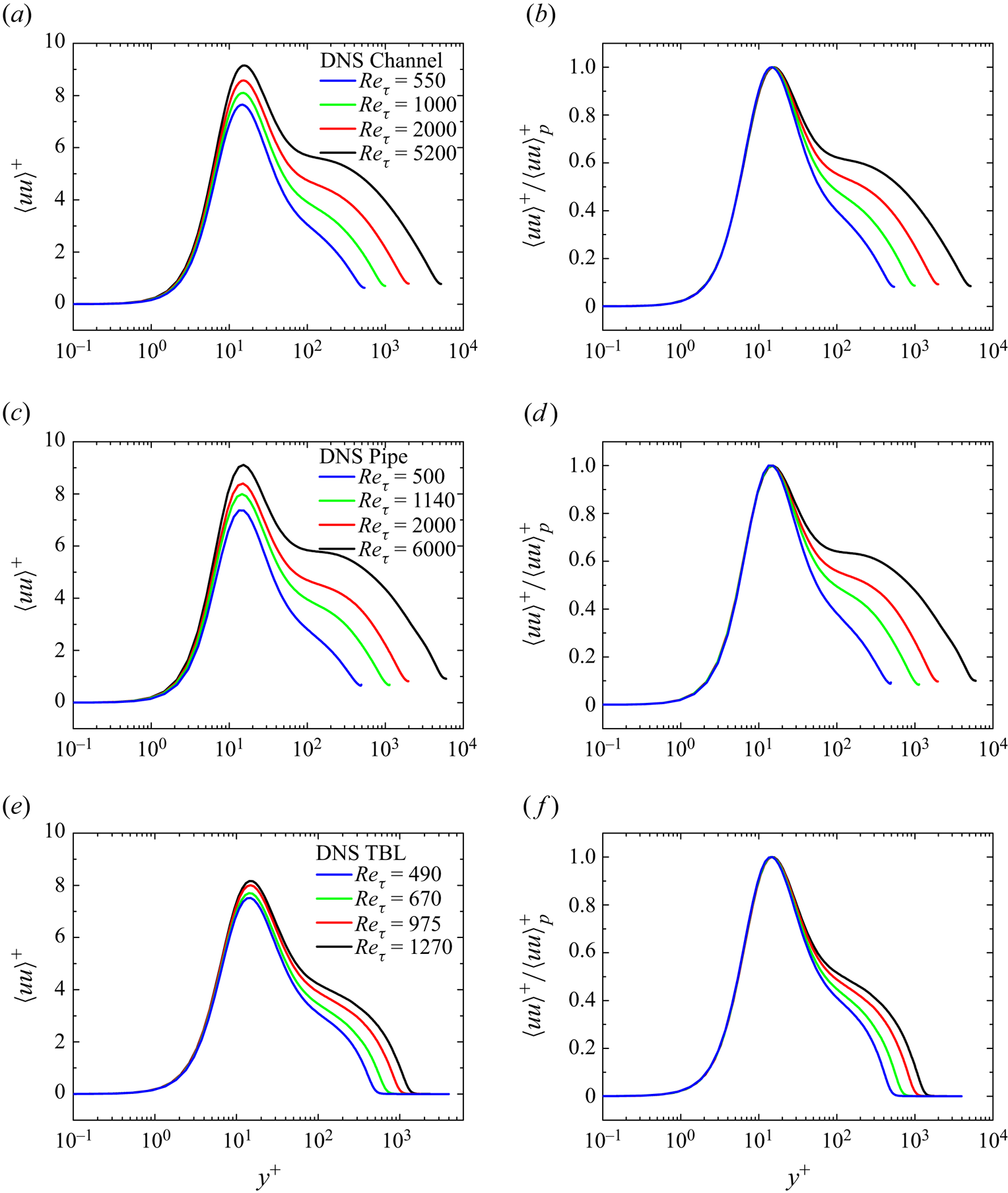
Figure 1. Wall-normal dependence of streamwise velocity fluctuation scaled in viscous units (abscissa in logarithmic scale) for a series of  $Re_\tau$s in (a,b) channels, (c,d) pipes and (e,f) TBL flows. (a,c,e) Here
  $\langle u u\rangle ^+$ versus
  $y^+$. (b,d,f) Here
  $\langle u u\rangle ^+$ normalized by its (inner) peak value
  $\langle u u\rangle ^+_p$, showing very good collapse. Coloured lines indicate DNS data at different
  $Re_\tau$s marked in the figure legends, for channels by Lee & Moser (Reference Lee and Moser2015), for pipes by Pirozzoli et al. (Reference Pirozzoli, Romero, Fatica, Verzicco and Orlandi2021) and for TBLs by Schlatter et al. (Reference Schlatter, Örlü, Li, Brethouwer, Fransson, Johansson, Alfredsson and Henningson2009, Reference Schlatter, Li, Brethouwer, Johansson and Henningson2010).
As for (2.2), data collapse for the spanwise velocity fluctuation is achieved via
 \begin{equation} \langle w w\rangle^+(y^+,Re_\tau)=\langle w w\rangle^+_p(Re_\tau) h(y^+), \end{equation}
where  $\langle w w\rangle ^+_p$ is the peak value, and
  $h$ is a
  $y^+$-dependent function. As shown in figure 2, different
  $Re_\tau$ curves are in close agreement with each other, with the self-preserving range from the wall to the peak (at
  $y^+\approx 45$) or beyond. We note a marginal
  $Re_\tau$ dependence on this peak location; it is hard to tell whether they arise from numerical uncertainty or physical modulation by outer flow structures. Since this variation is marginal, we shall not consider this any further.


Coming now to pressure fluctuations, figure 3(a,c,e) shows  $Re_\tau$ dependence of
  $p'^+$. The best collapse is obtained by plotting
  $p'^+_{p}-p'^+$, as shown in figure 3(b,d,f). On this basis, we may write
 \begin{equation} p'^+(y^+, Re_\tau)=p'^+_{p}(Re_\tau)-j(y^+), \end{equation}
where  $j$ is (in general) a
  $y^+$-dependent function. The collapse extends from the wall to the peak (at
  $y^+\approx 30$), with
  $p'^+_p-p'^+_w$ a constant around 0.4. This constancy inspires us to postulate (2.4). Instead, if one plots
  $p'^+/p'^+_{p}$, data would not collapse (not shown here). The reason is clear from (2.4), i.e.
  $p'^+/p'^+_{p}=1-j(y^+)/p'^+_{p}(Re_\tau )$: an increasing
  $p'^+_{p}$ with
  $Re_\tau$ would eventually spoil the data collapse of
  $p'^+/p'^+_{p}$. That is the reason why (2.2) or (2.3) is not applied to
  $p'^+$. Note that Panton et al. (Reference Panton, Lee and Moser2017) attempted another data collapse by using
  $\langle pp\rangle ^+_w-\langle pp\rangle ^+$, but it is not as satisfactory as (2.4) in figure 3, as also discussed later in § 3.

Figure 3. Wall-normal dependence for the r.m.s. of pressure fluctuation  $p'^+=\langle pp\rangle ^{+1/2}$ in (a,b) channels, (c,d) pipes and (e,f) TBL flows: (a,c,e)
  $p'^+$; (b,d,f)
  $p'^+_p-p'^+$ versus
  $y^+$. Lines are the same DNS data as in figure 1.
2.2. Summary for the near-wall scaling
The above comparisons demonstrate that the  $Re_\tau$ and
  $y^+$ dependencies could be decoupled after a proper normalization by peak values. Recalling (1.2) for the
  $Re_\tau$-scaling of the peak values and substituting it for
  $\langle uu\rangle ^+_p$,
  $\langle ww\rangle ^+_p$ and
  $p'^+_p$ into (2.2), (2.3) and (2.4), respectively, one has a uniform expansion, as reinforced for
  $\langle uu\rangle ^+$ also by Monkewitz (Reference Monkewitz2022), i.e.
 \begin{equation} \phi(y^+)=\phi_0(y^+)+\phi_1(y^+)/Re^{1/4}_\tau, \end{equation}
where  $\phi _0(y^+)=\phi _\infty f(y^+)$ and
 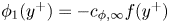 $\phi _1(y^+)=-c_{\phi, \infty } f(y^+)$ for
  $u$;
$u$;  $\phi _0(y^+)=\phi _\infty h(y^+)$ and
 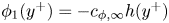 $\phi _1(y^+)=-c_{\phi, \infty } h(y^+)$ for
  $w$;
$w$;  $\phi _0(y^+)=\phi _\infty -j(y^+)$ and
  $\phi _1(y^+)=-c_{\phi, \infty }$ for pressure fluctuations.
Note that (2.5) is a specific case of
 \begin{equation} \phi(y^+,Re_\tau)=f_0(y^+)+f_1(y^+)g(Re_\tau), \end{equation}
which is a second-order truncation of (2.1), considered also by Spalart & Abe (Reference Spalart and Abe2021) and Monkewitz (Reference Monkewitz2022). If  $f_0=0$, (2.6) reduces to
 \begin{equation} \phi(y^+,Re_\tau)=f_1(y^+)g(Re_\tau), \end{equation}
which is the scaling proposed by Smits et al. (Reference Smits, Hultmark, Lee, Pirozzoli and Wu2021) for  $\langle uu \rangle ^+$ with
 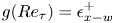 $g(Re_\tau )=\epsilon ^+_{x-w}$ (streamwise wall dissipation). However, Smits et al. (Reference Smits, Hultmark, Lee, Pirozzoli and Wu2021) found that their proposal did not work as well for
  $\langle w w\rangle ^+$, which they speculated was due to different superposition and modulation enforced by outer flow structures. Here, we show that replacing wall dissipation by peak value, i.e.
  $g=\phi _p$, (2.7) applies for both
  $\langle uu \rangle ^+$ and
  $\langle ww \rangle ^+$. Even so, (2.7) is not proper for pressure due to a constancy
  $p'^+_p-p'^+_w$ as explained earlier. The non-zero
  $f_0$ needed in (2.6) has been missed in the past.
Finally, we recall that from (2.6), Monkewitz (Reference Monkewitz2022) developed a composite model for  $\langle uu\rangle ^+$, which shows that
  $g=Re^{-1/4}_\tau$ yields a better data description than the alternative
  $g=\ln Re_\tau$ considered by Smits et al. (Reference Smits, Hultmark, Lee, Pirozzoli and Wu2021). The gauge function
  $g=Re^{-1/4}_\tau$ in (2.6) restores wall scaling for asymptotically high
  $Re_\tau$; we will use it below to derive an outer decay profile, which has not been achieved before.
3. The $Re_\tau$-scaling for the outer region and the defect law for fluctuations

Similar to (2.1) for the inner region, an asymptotic expansion for the outer flow reads
 \begin{equation} \phi(y^\ast,Re_\tau)=F_0(y^\ast)+F_1(y^\ast)G(Re_\tau)+F_2(y^\ast)G^2(Re_\tau)+{\rm h.o.t.}, \end{equation}
where  $y^\ast =y^+/Re_\tau$ is the outer unit;
  $F_0$,
  $F_1$ and
  $F_2$ are general functions depending on
  $y^\ast$, and
  $G(Re_\tau )$ is the gauge function. In analogy to law of the wall, the outer flow similarity corresponds to the first-order truncation in (3.1), i.e.
 \begin{equation} \phi(y^\ast,Re_\tau)=F_0(y^\ast). \end{equation}
When we take 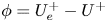 $\phi =U^+_e-U^+$, the resulting equation for the mean velocity is known as the velocity defect law. Here, the subscript
  $e$ indicates the value at
  $y^\ast =1$, i.e. the centreline for channel and pipe flows, and the boundary layer edge for TBL. This law has been explored extensively in the literature – see Nagib, Chauhan & Monkewitz (Reference Nagib, Chauhan and Monkewitz2007) and She, Chen & Hussain (Reference She, Chen and Hussain2017) for recent efforts. We shall now develop the equation for the fluctuating quantities.
An assessment of outer similarity for the three fluctuation profiles is shown in figure 4, with figure 4(a–c) for the channel, figure 4(d–f) for the pipe and figure 4(g–i) for the TBL. It is particularly remarkable that the pressure fluctuation displays an excellent data collapse from  $y^\ast =0.1$ to
  $y^\ast =1$. In the same flow region, the spanwise velocity variance data also collapse well, with a deviation of the order of 0.1 (scaled on
  $u^2_\tau$). For streamwise velocity, the outer similarity holds better towards the outer edge though discernible
  $Re_\tau$ dependence exists towards small
  $Re_\tau$. For
  $Re_\tau > 1000$, the streamwise variance profiles collapse together closely (figures 5 and 6), thus supporting the outer similarity of fluctuations for high
  $Re_\tau$.

Figure 4. Wall-normal dependence of turbulence fluctuations in outer length unit  $y^\ast =y/\delta$ (the abscissa in linear scale): (a–c) channels, (d–f) pipes and (g–i) TBLs; (a,d,g)
  $\langle uu\rangle ^+$; (b,e,h)
  $\langle ww\rangle ^+$; (c,f,i)
  $p'^+$. Lines are the same DNS data as in figure 1.
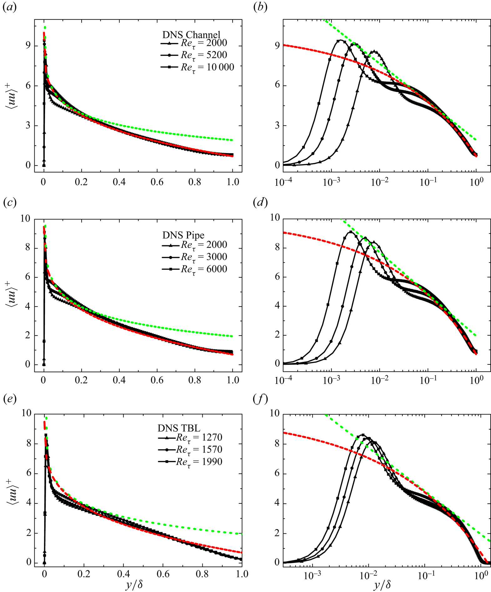
Figure 5. Variance of streamwise velocity fluctuation of DNS data at high  $Re_\tau$. Channel data in (a,b) are
  $Re_\tau =2000, 5200$ from Lee & Moser (Reference Lee and Moser2015),
  $Re_\tau =10^4$ from Hoyas et al. (Reference Hoyas, Oberlack, Alcantara-Avila, Kraheberger and Laux2022). Pipe data in (c,d) from Pirozzoli et al. (Reference Pirozzoli, Romero, Fatica, Verzicco and Orlandi2021). Panels (e,f) for TBL,
  $Re_\tau =1270$ from Schlatter & Örlü (Reference Schlatter and Örlü2010),
  $Re_\tau =1570,1990$ from Sillero et al. (Reference Sillero, Jimenez and Moser2013). Here (a,c,e) is for abscissa in linear and (b,d,f) in logarithmic outer units
  $y^\ast =y/\delta$, to highlight wall-normal distances close to the wall. Dotted (green) line in (a,b) indicates
  $1.61-1.25\ln y^\ast$ by Hultmark et al. (Reference Hultmark, Vallikivi, Bailey and Smits2012);
  $2.2-1.26\ln y^\ast$ in (c,d) by Marusic et al. (Reference Marusic, Monty, Hultmark and Smits2013) and
  $1.95-1.26\ln y^\ast$ in (e,f) by Samie et al. (Reference Samie, Marusic, Hutchins, Fu, Fan, Hultmark and Smits2018). Dashed (red) lines indicate the present relation (1.3), i.e.
  $10-9.3y^{\ast 1/4}$, the same for all the flows here.
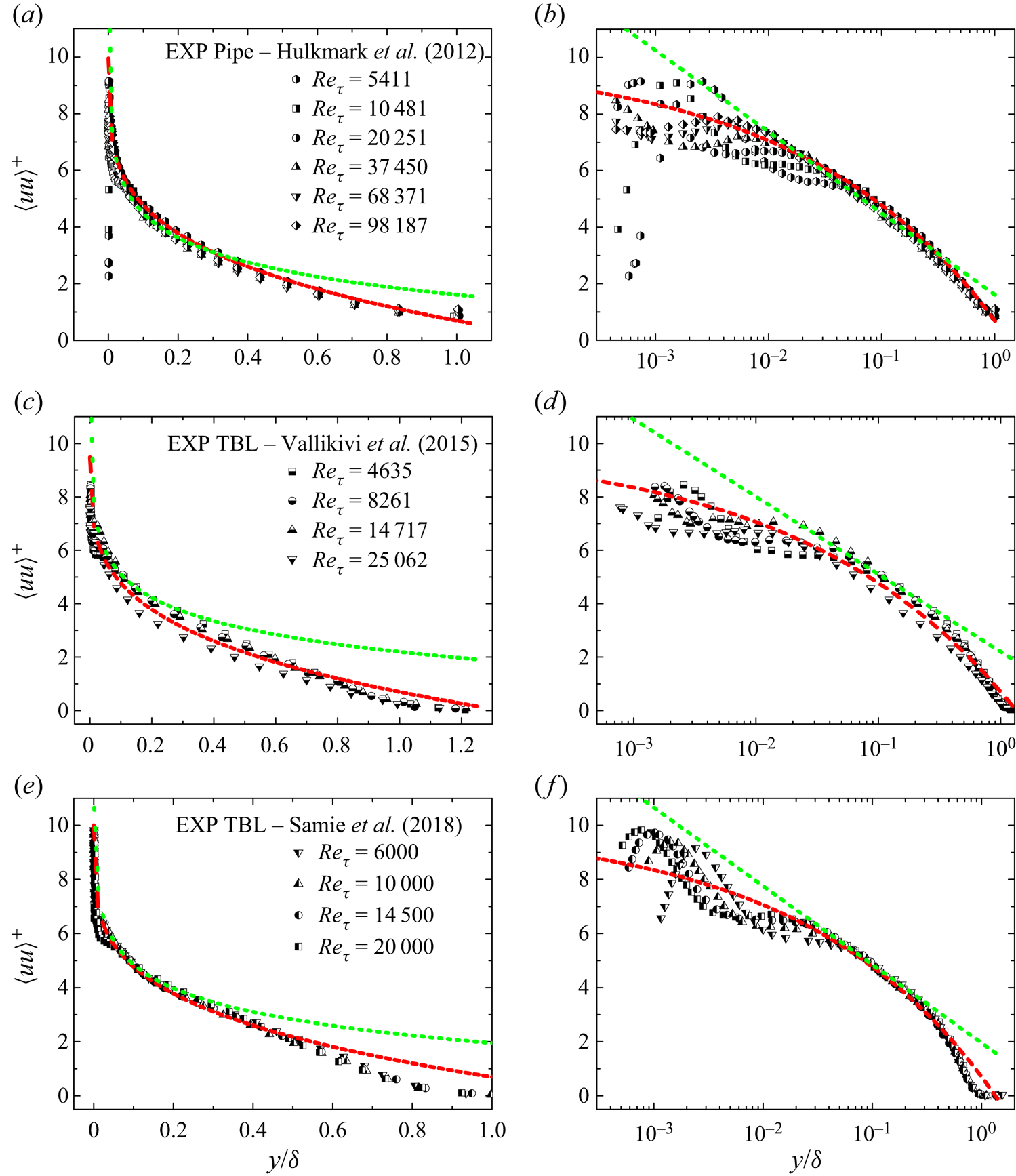
Figure 6. Variance of streamwise velocity fluctuation in high  $Re_\tau$ experiments. Data in (a,b) from Princeton pipe (Hultmark et al. Reference Hultmark, Vallikivi, Bailey and Smits2012), (c,d) from Princeton TBL (Vallikivi et al. Reference Vallikivi, Ganapathisubramani and Smits2015) and (e,f) from Melbourne TBL (Samie et al. Reference Samie, Marusic, Hutchins, Fu, Fan, Hultmark and Smits2018). Dotted (green) line in (a,b) indicates
  $1.61-1.25\ln y^\ast$ by Hultmark et al. (Reference Hultmark, Vallikivi, Bailey and Smits2012);
  $2.2-1.26\ln y^\ast$ in (c,d) by Marusic et al. (Reference Marusic, Monty, Hultmark and Smits2013) and
  $1.95-1.26\ln y^\ast$ in (e,f) by Samie et al. (Reference Samie, Marusic, Hutchins, Fu, Fan, Hultmark and Smits2018). Dashed (red) lines indicate (1.3), i.e.
 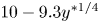 $10-9.3y^{\ast 1/4}$ in all the panels (here
  $y^\ast =y/\delta$).
3.1. Matching for the defect law for fluctuations
Based on the above inner expansion and outer similarity, we now develop a matching procedure to derive the analytical form in the intermediate zone. One may invoke the derivation of Millikan (Reference Millikan1938) for the log law in the mean velocity distribution, which has been extended for  $\langle uu\rangle ^+$ by Hultmark (Reference Hultmark2012) and for
  $\langle p p\rangle ^+$ by Panton et al. (Reference Panton, Lee and Moser2017). Nevertheless, different orders of matching would lead to different scaling proposals, and here we present a short account of matching to obtain the defect law for fluctuations.
As a starting point, we note an exact matching between the inner and outer flows for the total stress in channels or pipes. That is,  $\tau ^+(y^+,Re_\tau )=1-y^+/Re_\tau$, which can be rewritten as
  $\tau ^+(y^\ast,Re_\tau )=1-y^\ast$. The first version of
  $\tau ^+(y^+,Re_\tau )$ corresponds to the two-term inner expansion of (2.6) with
  $\phi =\tau ^+$,
  $f_0(y^+)=1$,
  $f_1(y^+)=y^+$ and
  $g=Re^{-1}_\tau$; the second version of
  $\tau ^+(y^\ast,Re_\tau )$ corresponds to the one-term expansion in (3.1), or to the outer similarity in (3.2) with
  $\phi =\tau ^+$ and
  $F_0(y^\ast )=1-y^\ast$. Thus, the total stress satisfies a straightforward matching between (2.6) and (3.2), i.e.
  $f_0(y^+)+f_1(y^+)g(Re_\tau )=F_0(y^\ast )$, valid for the entire flow, quite unlike Millikan's matching analysis that requires
  $1/Re_\tau \ll y^\ast \ll 1$ (or
  $1\ll y^+\ll Re_\tau$) and dictates a term-by-term balance.
Therefore, we match (2.6) directly with (3.2), i.e. 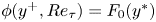 $\phi (y^+,Re_\tau )=F_0(y^\ast )$, and obtain
 \begin{align} \phi(y^+,Re_\tau)&=f_{0}(y^+)+f_{1}(y^+)/Re^{1/4}_\tau\nonumber\\ &=f_{0}(y^+)+{h}_{1}(y^+)y^{{\ast1/4}}\nonumber\\ &=F_0(y^\ast) \end{align}
(where  $g=Re_\tau ^{-1/4}$ is used and
  ${h}_{1}(y^+)=f_1(y^+)/y^{+1/4}$). Note that
  $f_{0}=\phi _0$ and
  $h_{1}=\phi _{1}/y^{+1/4}$ as the wall is approached, so that (3.3) approaches (2.5), but
  $f_0$ and
  $h_1$ towards the outer region are to be determined. At this stage, as
  $F_0(y^\ast )$ in (3.3) depends only on
  $y^\ast$, we have
 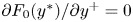 $\partial F_0(y^\ast )/\partial y^+=0$ in (3.3), and hence
 \begin{gather} f_{0}(y^+)=c_0, \end{gather}
 \begin{gather} {h}_{1}(y^+)=c_1, \end{gather}
where  $c_0$ and
  $c_1$ are constants independent of
  $y^\ast$,
  $y^+$ and
  $Re_\tau$, but may depend on the variable
  $\phi$. Denoting
  $c_0=\alpha _\phi$ and
  $c_1=-\beta _\phi$, we obtain (1.3) from (3.3) and (3.4). It is readily verified that (1.3) matches (3.2) in the outer region and (2.6) in the inner, hence offers a common description connecting the two.
In the above procedure, we have assumed that the two-term expansion  $f_{0}(y^+)+f_{1}(y^+)g(Re_\tau )$ extends to the outer flow, so that it matches with
  $F_0(y^\ast )$ and satisfies the outer similarity as well. As explained above, the procedure works exactly for the total stress in channels and pipes with
  $g=Re^{-1}_\tau$.
3.2. Comparison with the data
Figures 5–8 show comparisons of data with (1.1) and (1.3) for  $\langle uu\rangle ^+$,
  $\langle ww\rangle ^+$ and
  $p'^+$, respectively. Table 1 collects all the parameters for the three profiles, arising from these fits to the data, which we now discuss.
Table 1. Parameters in (1.3), for different fluctuations. Superscripts ‘CH’, ‘Pipe’ and ‘TBL’ represent channel, pipe and boundary layer flows, respectively. Note that both  $\alpha _\phi$ and
  $\beta _\phi$ vary only modestly among different flows, implying that essentially the same mechanisms applies for all flows. Moreover,
  $\beta _\phi$ is quite close to
  $\alpha _\phi$, as
  $\phi$ at the boundary layer edge
  $y^\ast =1$ is fairly small.

Similar to figures 1–3, figures 5(a,b), 6(a,b), 7(a,b) and 8(a,b) are for channel, figures 5(c,d), 6(c,d), 7(c,d) and 8(c,d) for pipe and figures 5(e,f), 6(e,f), 7(e,f) and 8(e,f) for boundary layers; for figures 5(a,c,e), 6(a,c,e), 7(a,c,e) and 8(a,c,e) the abscissa are in linear units while for figures 5(b,d,f), 6(b,d,f), 7(b,d,f) and 8(b,d,f), logarithmic units are used. A difference from figures 1–3 is that the data in figures 5–8 are denoted by black symbols, so that (1.1) and (1.3) are better marked to guide the eye.

Figure 7. Variance of spanwise velocity fluctuation in channel (a,b), pipe (c,d) and TBL (e,f) flows scaled in outer units  $y^\ast =y/\delta$. Dashed (red) lines indicate the bounded decay (1.3) with parameters in table 1. Dotted (green) lines indicate the logarithmic decay (1.1), i.e.
 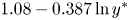 $1.08-0.387\ln y^\ast$ for channel and pipe, and
  $1.23-0.387\ln y^\ast$ for TBL. Symbols with lines are the same DNS data as in figure 1, i.e. channel from Lee & Moser (Reference Lee and Moser2015), pipe from Pirozzoli et al. (Reference Pirozzoli, Romero, Fatica, Verzicco and Orlandi2021), TBL from Schlatter et al. (Reference Schlatter, Örlü, Li, Brethouwer, Fransson, Johansson, Alfredsson and Henningson2009, Reference Schlatter, Li, Brethouwer, Johansson and Henningson2010).

Figure 8. The r.m.s. of pressure fluctuation in channel (a,b), pipe (c,d) and TBL (e,f) flows scaled in the outer unit  $y^\ast =y/\delta$. Dashed (red) lines indicate the bounded decay (1.3) with parameters in table 1. Dotted (green) lines indicate the logarithmic decay in (3.5), i.e.
  $\sqrt {0.27-2.56\ln y^\ast }$ for channel,
  $\sqrt {0.6-2.45\ln y^\ast }$ for pipe and
  $\sqrt {2.5-2.45\ln y^\ast }$ for TBL. Symbols with lines are the same DNS data as in figure 7.
Particularly for  $\langle uu\rangle ^+$, to avoid distractions by data scatter at small
  $Re_\tau$, we collect in figure 5 only high
  $Re_\tau$ profiles from DNS, namely,
  $Re_\tau$ from
  $2000$ to
  $10^4$ for channel; 2000 to 6000 for pipe; and 1270 to 1990 for TBL. Compared with figure 4(a,d,g), it is clear in figure 5(a,c,e) that all high
  $Re_\tau$ profiles collapse on each other in the flow range
  $0.1\lesssim y^\ast \lesssim 1$, thus bearing witness to outer similarity. This is confirmed again by experimental data in figure 6 corresponding to higher
  $Re_\tau$.
Note that the logarithmic behaviour advanced in the literature (Hultmark et al. Reference Hultmark, Vallikivi, Bailey and Smits2012; Marusic et al. Reference Marusic, Monty, Hultmark and Smits2013; Samie et al. Reference Samie, Marusic, Hutchins, Fu, Fan, Hultmark and Smits2018) is indicated by a green dotted line. Although it characterizes data in the region from  $0.1\lesssim y^\ast \lesssim 0.3$, the value of the intercept
  $B_\phi$ needs to be adjusted for the three flows from 1.61 to 2.2, while
  $A_\phi$ holds constant around 1.26. In contrast, the red dashed line represents (1.3) with the same
  $\alpha _\phi =10$ and
  $\beta _\phi =9.3$, which reproduces data well for channel, pipe and TBL flows, covering not only the logarithmic range (vis-à-vis the mean flow) but also the so-called wake region, almost all the way to the centreline of channel and pipe flows.
One may imagine that the data in figure 5 have not reached the asymptotic state and that (1.1) might agree with data better for higher  $Re_\tau$. But experimental data from Princeton pipes (Hultmark et al. Reference Hultmark, Vallikivi, Bailey and Smits2012) with
  $Re_\tau$ covering one more decade, e.g.
  $Re_\tau$ from approximately
  $5000$ to
  $10^5$, do not show any improvement of the fit to (1.1) (see figure 6a,b). A similar observation is also true for the TBL, as shown in figure 6(c–f).
Likewise, for  $\langle ww\rangle ^+$ and
  $p'^+$, (1.3) extends almost all the way to the centreline of channel and pipe flows. Here, data in figures 7 and 8 are the same DNS groups as in figure 1 and contain those low
  $Re_\tau$ profiles. The agreement with (1.3) is excellent at the smallest
  $Re_\tau \approx 500$ for channel and pipe, in contrast to the log variation that agrees with data only for
  $Re_\tau \gtrsim 2000$. Therefore, in both
  $y$ and
  $Re_\tau$ ranges, (1.3) covers a wider range than (1.1).
Three further points will now be discussed. First, the difference between (1.3) and (1.1) is more vital for asymptotically high  $Re_\tau$. For (1.1), an infinitely large of
  $\phi \propto \ln Re_\tau$ would arise as
  $y^\ast \rightarrow 0$ and
  $Re_\tau \rightarrow \infty$. In contrast, (1.3) assigns a plateau of
  $\phi \approx \alpha _\phi$ in the same limit. Such an asymptotic plateau implies that turbulent eddies in the bulk would be in a quasiequilibrium state in the sense that their contribution to
  $\phi$ is invariant when
  $y$ changes. Note also that according to (1.3), the outer peak of
  $\langle uu\rangle ^+$, if it exists, should be bounded by
  $\langle uu\rangle ^+\approx 10$. Clarification of such differences of perspectives in the asymptotic state require data at higher Reynolds numbers.
Second, while (1.3) adheres closely with TBL data of Vallikivi et al. (Reference Vallikivi, Ganapathisubramani and Smits2015) up to  $y^\ast =1$ (figure 6c), it is slightly and uniformly higher than the TBL data of Samie et al. (Reference Samie, Marusic, Hutchins, Fu, Fan, Hultmark and Smits2018) for
  $y^\ast >0.6$ (figure 6e). This is due to the fact that the former set of data are obtained for flow over a flat plate mounted in the same pipe in which data of Hultmark et al. (Reference Hultmark, Vallikivi, Bailey and Smits2012) are measured. Therefore, the data of Vallikivi et al. (Reference Vallikivi, Ganapathisubramani and Smits2015) in its outer wake region resemble the centre behaviour of pipe data by Hultmark et al. (Reference Hultmark, Vallikivi, Bailey and Smits2012), both in agreement with (1.3) up to
  $y^\ast =1$. In contrast, TBL data of Samie et al. (Reference Samie, Marusic, Hutchins, Fu, Fan, Hultmark and Smits2018) are measured in the Melbourne wind tunnel with the standard free stream boundary condition, so that a vanishing
  $\langle uu\rangle ^+\approx 0$ towards the boundary layer edge is observed (figure 6e,f), which is lower than (1.3). This difference reflects the wake influence on
  $\langle uu\rangle ^+$ in TBL. In fact, the wake influence is much sharper for
  $\langle ww\rangle ^+$ and
  $p'^+$ in TBL (figures 7e and 8e). This issue will be addressed in § 4.2.
The third point is that, for  $p'^+$, the green dotted line in figure 8 represents
 \begin{equation} p'^+(y^\ast)=\sqrt{ B_{\phi}-A_{\phi} \ln y^\ast }, \end{equation}
which is the square root of (1.1) for pressure variance
 \begin{equation} \langle pp\rangle^+(y^\ast)={ B_{\phi} - A_{\phi} \ln y^\ast}. \end{equation}
This equation is obtained by Panton et al. (Reference Panton, Lee and Moser2017) via an inner–outer matching (i.e. a viscous inner layer overlapping with an inviscid outer layer). It is almost indistinguishable from (1.3) in figure 8. Nevertheless, as shown in figure 9(a–c),  $\langle pp\rangle ^+_w-\langle pp\rangle ^+$ versus
  $y^+$ produces no data collapse for
  $y^+>5$. Particularly for the trough located at approximately
  $y^+=30$, the data are markedly lower for increasing
  $Re_\tau$, thus creating a challenge for the inner–outer matching analysis. To reconcile this challenge, Panton et al. (Reference Panton, Lee and Moser2017) introduced two logarithmic slopes, i.e.
  $A^{CP}=2.56$ for the common part of presumed log profile in the overlap layer, and another
  $A^{w}=2.24$ for the
  $Re_\tau$ variation of the wall pressure. Following this fix, one can estimate
 \begin{equation} \langle pp\rangle^+_p-\langle pp\rangle^+_w\propto (A^{CP}-A^{w})\ln Re_\tau\approx 0.32\ln Re_\tau, \end{equation}
which would break the wall scaling completely.

Figure 9. Wall-normal dependence of the variance of pressure fluctuations is shown in the plots of  $\langle pp\rangle ^+_w-\langle pp\rangle ^+$ versus
  $y^+$, where
  $\langle pp\rangle ^+_w$ is the wall-value of
  $\langle pp\rangle ^+$. Lines are the same DNS data as in figure 3: (a) channels; (b) pipes; (c) TBLs. Note that lines depart markedly from each other with increasing
  $Re_\tau$ in the region
  $y^+>5$. (d) Difference between the peak and wall values of pressure variance, i.e.
  $\langle pp\rangle ^+_p-\langle pp\rangle ^+_w$, for channel, pipe and TBL flows for a series of
  $Re_\tau$ values. Dotted line (green) indicates the logarithmic growth by (3.7), i.e.
 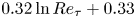 $0.32\ln Re_\tau +0.33$. Dashed line (red) indicates the bounded variation of (3.8) according to CS. Symbols are DNS data, squares for channel (Lee & Moser Reference Lee and Moser2015), circles for pipe (Pirozzoli et al. Reference Pirozzoli, Romero, Fatica, Verzicco and Orlandi2021) and diamonds for TBL (Schlatter et al. Reference Schlatter, Örlü, Li, Brethouwer, Fransson, Johansson, Alfredsson and Henningson2009). Note that DNS channel data at
  $Re_\tau =150, 300, 400$ of Iwamoto, Suzuki & Kasagi (Reference Iwamoto, Suzuki and Kasagi2002), and
  $Re_\tau =180, 550, 944, 2000$ of Hoyas & Jimenez (Reference Hoyas and Jimenez2006) are also included here.
As a comparison, figure 3(b,d,f) show that data of  $p'^+_w-p'^+$ collapsed well up to the trough, better than
  $\langle pp\rangle ^+_w-\langle pp\rangle ^+$ in figure 9(a–c). Moreover, via the bounding relation
 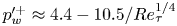 $p'^+_w\approx 4.4-10.5/Re^{1/4}_\tau$ and
 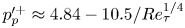 $p'^+_p\approx 4.84-10.5/Re^{1/4}_\tau$ given in CS, we have
 \begin{equation} \langle pp\rangle^+_p-\langle pp\rangle^+_w=p'^{{+}2}_p-p'^{{+}2}_w\approx4.07-9.24/Re_\tau^{1/4}, \end{equation}
which depicts data satisfactorily over a wider  $Re_\tau$ range than (3.7) in figure 9(d).
Finally, to evaluate the goodness of the theoretical fits with the data, taking the channel at  $Re_\tau =5200$ (Lee & Moser Reference Lee and Moser2015) for example, we have calculated the variance of difference between DNS data (
 $\phi _{Data}$) and theoretical predictions (
 $\phi _{Eq}$), i.e.
  $\sigma ^2 = \sum _{0.1 \le {y^\ast _i} \le 1} {{{[\phi _{Data}({y^\ast _i}) - \phi _{Eq} ({y^\ast _i})]}^2}} /N$ where
  $N$ is the total number of data points in the range from
  $y^\ast =0.1$ to
  $y^\ast =1$. For (1.3),
  $\sigma ^2$ is
  $0.007$ for
  $\langle uu\rangle ^+$,
  $0.002$ for
  $\langle ww\rangle ^+$ and
  $0.002$ for
  $p'^+$; while for (1.1),
  $\sigma ^2$ is
  $0.26$,
  $0.14$ and
  $0.004$ for
  $\langle uu\rangle ^+$,
  $\langle ww\rangle ^+$ and
  $p'^+$, respectively. The larger
  $\sigma ^2$ of (1.1) for
  $\langle uu\rangle ^+$ and
  $\langle ww\rangle ^+$ is not surprising because of their deviation from data towards the centreline. But we should remember that (1.1) is derived for asymptotically high
  $Re_\tau$ and is not supposed to depict the data behaviour towards
  $y^\ast =1$. In this sense,
  $1/Re_\tau \ll y^\ast \ll 1$ might be better for the competition between the two proposals, but that would lose sight of the advantage that (1.3) covers a wider outer domain.
3.3. Brief critique of the matching arguments
Two further points will be considered here. Despite the agreement with the data, one should note that, according to (1.3),  $\partial \phi /\partial y^\ast =-\beta _\phi /4$ at
  $y^\ast =1$, which is against the mirror symmetry of
  $\partial \phi /\partial y^\ast =0$ at the centreline of channel and pipe. This indicates that there is a discrepancy between (1.3) and data towards the centreline, for which a centre core layer or the wake modification is needed, as shown in Monkewitz (Reference Monkewitz2023).
Secondly, a perusal of the fits with data suggests the existence of a gap between the inner peak and the outer data collapse, particularly for  $\langle uu\rangle ^+$ (figure 1b,d,f). This indicates a modest
  $Re_\tau$-dependence even after normalization by the peak. This may also be the influence of higher-order terms in (2.1), as explained here by the two-term expansion. From (2.6), we expand
 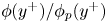 $\phi (y^+)/\phi _p(y^+)$ by the parameter
  $g(Re_\tau )$; that is,
 \begin{equation} \frac{{\phi ({y^ + })}}{{\phi (y_p^ + )}} = \frac{{{f_0}({y^ + })}}{{{f_0}(y_p^ + )}}\left\{ {1 + \left[ {\frac{{{f_1}({y^ + })}}{{{f_0}({y^ + })}} - \frac{{{f_1}(y_p^ + )}}{{{f_0}(y_p^ + )}}} \right]g({{Re}_\tau }) + \cdots} \right\}. \end{equation}
When  $f_0(y^+)$ and
  $f_1(y^+)$ are proportional to each other, one has
  ${f_1}({y^ + })/{f_0}({y^ + }) - {f_1}({y^ + _p})/{f_0}({y^ + _p}) = 0$, and hence
  $\phi ({y^ + })/\phi ({y^ +_p })$ from (3.9) is independent of
  $g(Re_\tau )$. This case corresponds to the data collapse of
  $\langle uu\rangle ^+$ from the wall to the peak. However, when
  $f_0(y^+)$ and
  $f_1(y^+)$ are no longer proportional to each other, the gauge function
  $g(Re_\tau )$ in (3.9) indicates that (3.9) still has
  $Re_\tau$-dependence, which corresponds to the gap between the inner peak and the outer approximation (1.3). Therefore, the proportionality or otherwise of
  $f_0(y^+)$ and
  $f_1(y^+)$ in (2.6) would determine the data collapse or slight mismatch when plotting via
  $\phi ({y^ + })/\phi ({y^ +_p })$. There is no stipulation here that the ratio of
  $f_0(y^+)$ to
  $f_1(y^+)$ is constant in matching (3.3). In fact, according to (3.4),
  $f_0(y^+)/f_1(y^+)=c_0/(c_1y^{+1/4})$. Therefore, even if
  $f_0$ and
  $f_1$ are not proportional to each other, we can still match (2.6) with (3.2) to obtain (3.3).
4. Discussion on the influence of flow geometry
4.1. Near wall universality
We focus here on the geometry effects. First, a universal data collapse is summarized by unifying (2.2), (2.3) and (2.4) together, i.e.
 \begin{equation} \frac{\phi(y^+,Re_\tau)-\phi_w(Re_\tau)}{\phi_p(Re_\tau)-\phi_w(Re_\tau)}= f_\phi(y^+), \end{equation}
where  $f_\phi (y^+)$ depends on
  $y^+$ and
  $\phi$ but is independent of
  $Re_\tau$. For
  $\langle uu\rangle ^+$,
  $\phi _w=0$ so that (4.1) reduces to (2.2); the same is true for
  $\langle ww\rangle ^+$. For
  $p'^+$, as
  $\phi _p-\phi _w$ is a constant independent of
  $Re_\tau$ shown in figure 3, (4.1) reproduces (2.4) with
  $f_\phi =1-j(y^+)/j(0)$.
Moreover, as  $y^+$ moves from the wall to the peak location, it is interesting to check whether
  $f_\phi (y^+)$ is universal for channel, pipe and TBL flows. This is indeed verified in figure 10(a–c), for
  $\langle uu\rangle ^+$,
  $\langle ww\rangle ^+$ and
  $p'^+$, respectively. Profiles from these three wall flows collapsed together from the wall to the peak location, which means that
  $Re_\tau$-dependence and geometry influence are cancelled by the ratio of relative variations composed of
  $\phi _w$ and
  $\phi _p$. This is conceivable if the near-wall region is viewed as a self-organized entity, so that superposition and modulation effects enforced by the outer flow structures are characterized to the first order by wall and peak values.

Figure 10. Wall-normal dependence for fluctuations after normalization by the corresponding peaks: (a)  $\langle uu\rangle ^+/\langle uu\rangle ^+_p$; (b)
  $\langle ww\rangle ^+/\langle ww\rangle ^+_p$; (c)
 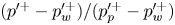 $(p'^+-p'^+_w)/(p'^+_p-p'^+_w)$. Lines are DNS data of channel at
  $Re_\tau =1000$ (Lee & Moser Reference Lee and Moser2015), of pipe at
  $Re_\tau =1140$ (Pirozzoli et al. Reference Pirozzoli, Romero, Fatica, Verzicco and Orlandi2021) and of TBL at
  $Re_\tau \approx 1270$ (Schlatter et al. Reference Schlatter, Li, Brethouwer, Johansson and Henningson2010), all of which collapse closely on each other near the wall.
4.2. Wake modification in TBL
Note that in figures 7 and 8,  $\langle ww \rangle ^+$ and
  $p'^+$ depart from (1.3) for
  $y^\ast \gtrsim 0.5$ in TBL, but the agreement persists all the way to the centreline of channel and pipe flows. Recall the findings by Chen, Hussain & She (Reference Chen, Hussain and She2019) that the total shear stress
  $\tau ^+$ and the Reynolds shear stress
  $\langle -uv\rangle ^+$ in the wake of the TBL differ notably from that in channel and pipe flows. The reason for this difference, according to Chen et al. (Reference Chen, Hussain and She2019), is the non-zero mean momentum transport in the wall-normal direction of TBL, i.e.
  $V/V_e\propto y^{\ast 3/2}$ (the subscript
  $e$ indicates the value at the boundary layer edge, as noted earlier), which offers a power law modelling for the
  $V$ profile in the bulk region. The latter leads to
  $\langle -uv\rangle ^+\approx \tau ^+\approx 1-y^{\ast 3/2}$ in TBL, differing from
  $\langle -uv\rangle ^+= 1-y^\ast$ in channel and pipe flows for which
  $V \equiv 0$.
Once we accept the difference in the  $\langle -uv\rangle ^+$ behaviour, we may expect a similar wake modification on
  $\langle ww \rangle ^+$ and
  $p'^+$ by the non-zero
  $V$ in TBL; that is,
 \begin{equation} \phi-\phi_e\propto \phi_{uv}-\phi_{uv,e}, \end{equation}
where  $\phi$ represents
  $\langle ww \rangle ^+$ or
  $p'^+$, and
  $\phi _{uv}$ represents
  $\langle -uv\rangle ^+$. If so, substituting
  $\phi _{uv}\approx 1-y^{\ast 3/2}$ into (4.2) yields
 \begin{equation} \phi(y^\ast)-\phi_e=c_{\phi} (\phi_{uv}-\phi_{uv,e})\approx c_{\phi}(1-y^{\ast3/2}), \end{equation}
where the proportionality coefficient  $c_{\phi }$ is independent of
  $y^\ast$ but may depend on
  $\phi$.
Verification of (4.3) for TBL is provided in figure 11. The agreement with the data is quite satisfactory for  $y^\ast >0.2$, and the fitting parameters are
  $\phi _e=0$ and
  $c_{\phi }=2.02$ for
  $\langle ww\rangle ^+$, while
  $\phi _e=0.8$ and
  $c_{\phi }=1.8$ for
  $p'^+$. This model for the wake flow could also be applied to describe
  $\langle uu \rangle ^+$ towards the free stream of the TBL, but the deviation is fairly small as shown in figures 5(e) and 6(e). Monkewitz & Nagib (Reference Monkewitz and Nagib2023) have shown a different behaviour of
  $\langle uu \rangle ^+$ and
  $U^+$ profiles in the TBL compared with channel and pipe flows using scaling indicator function, which implies different flow physics between external and internal flows.


5. Perspective and conclusions
New methods of analysis and generations of new experiments and simulations have revealed deeper and interesting questions on wall flow dynamics. Previously unthinkable questions, such as the universality of the Kármán constant in the mean flow description (Nagib et al. Reference Nagib, Monkewitz, Mascotelli, Fiorini, Bellani, Zheng and Talamelli2017; Monkewitz & Nagib Reference Monkewitz and Nagib2023) and the scaling of fluctuations in these flows, as well as the implications of the behaviour of fluctuations for the mean velocity itself, can now be asked, and reasonable answers for them can be attempted. In contrast to the mean velocity, concerted effort to understand the scaling of fluctuations is relatively new. This paper, when taken together with our earlier work (Chen & Sreenivasan Reference Chen and Sreenivasan2021, Reference Chen and Sreenivasan2022a), provides a self-consistent description of fluctuations in streamwise and spanwise velocity, as well as pressure fluctuations. One of the main qualitative conclusions of this work is that wall-normalized fluctuations are bounded even when  $Re_\tau \to \infty$, thus restoring the validity of the standard law of the wall. The alternative scenario of attached-eddy hypothesis and its consequences lead to a different conclusion.
We should reiterate that there exists no rigorous proof of either (1.1) or (1.3). The first step in establishing such a proof might be to justify the boundedness or otherwise of the peak values. An expansion analysis like that of Monkewitz & Nagib (Reference Monkewitz and Nagib2015) is highly desired, but how to choose a correct expansion parameter from first principles is currently unclear. Similarly, the quasilinear approximation by Hwang & Eckhardt (Reference Hwang and Eckhardt2020) is of also interest, as such an approach could reveal with much less computation the asymptotic feature of the Navier–Stokes equations as  $Re_\tau \rightarrow \infty$. There are significant issues for future study.
Aiming for an asymptotic description of fluctuations in canonical wall flows, we have obtained several new results, summarized as follows. First, excellent data collapse is achieved for the near-wall r.m.s. profiles of streamwise and spanwise velocity fluctuations ( $\langle uu\rangle ^+$ and
  $\langle ww\rangle ^+$) as well as pressure fluctuations (
 $p'^+$). Their spatial variations and the Reynolds number dependence are decoupled via the normalization through peak values. With the defect law for the peaks given in CS, a universal near-wall expansion (2.6) is obtained with the specific gauge function
  $g=Re^{-1/4}_\tau$.
Moreover, a defect decay (1.3) is derived by matching (2.6) with the outer similarity (3.2). Compared with the log profile by Townsend's attached-eddy hypothesis, it is shown that (1.3) reproduces the data better, not only over a wider  $Re_\tau$ domain but also in a larger flow region. As indicated by (1.3), there would appear an asymptotic plateau as
  $y^\ast \rightarrow 0$ and
  $Re_\tau \rightarrow \infty$, which implies a quasiequilibrium state with contributions to fluctuations coming from all associated eddies that are invariant as wall-normal position changes. If so, the intriguing outer peak of streamwise fluctuation, if one exists, would be bounded by
  $\langle uu\rangle ^+\approx 10$.
Finally, a near-wall universality (4.1) is obtained independent of both Reynolds number and flow geometries. In addition, a wake flow modification in TBL is introduced for  $\langle ww\rangle ^+$ and
  $p'^+$, which shows close agreement with data towards the boundary layer edge.
There is no gainsaying that more and better data are required to put all these results on a firmer foundation. It is exciting to await cleaner data at higher Reynolds numbers with improved resolution.
Acknowledgement
We thank all the authors cited in the figures for making their data available. We appreciate the suggestion of P. Monkewitz on the analysis leading to (3.9).
Funding
X.C. acknowledges the support by the National Natural Science Foundation of China (grant numbers 12072012, 92252201 and 11721202); and the Fundamental Research Funds for the Central Universities.
Declaration of interests
The authors report no conflict of interest.


 Open access