2. Experimental set-up

The experiments were conducted at the high pressure convection facility (HPCF) at the Max-Planck-Institute for Dynamics and Self-Organization in Göttingen. The convection cell has been described in detail before in previous publications (see e.g. Ahlers, Funfschilling & Bodenschatz Reference Ahlers, Funfschilling and Bodenschatz2009a; Ahlers et al. Reference Ahlers, He, Funfschilling and Bodenschatz2012b). Here, we use the version HPCF-II, which consists of a cylinder of height $H=2.24\ \textrm {m}$ and a diameter $D=1.12\ \textrm {m}$, resulting in an aspect ratio of $\varGamma =D/H=0.50$. The sidewall of the cylinder was made of a 9.5 mm thick acrylic. The top and bottom plates were made of high-purity copper with a heat conductivity of $394\ \textrm {W}\,\textrm {m}^{-1}\,\textrm {K}^{-1}$. The bottom plate consisted of two such copper plates (35 mm and 25 mm thick), separated by a 5 mm thin Lexan plate in between. The temperature drop across the Lexan plate was used to determine the vertical heat flux.

The bottom plate was heated with an ohmic heater at its bottom side, whereas the top plate was cooled using a circulated water bath which was temperature controlled with a precision of 0.02 K. Thermal shields underneath the bottom plate and around the sidewall ensured minimal heat loss through the bottom and the sides. Additional micro-shields close to the boundary layers at top and bottom aimed to reduce the heat transport through the sidewall close to the vertical boundaries (Ahlers Reference Ahlers2000; Stevens, Lohse & Verzicco Reference Stevens, Lohse and Verzicco2014).

The cell was mounted on a rotating table that could sustain an axial load up to 2800 kg. The table was driven by a direct drive motor (Siemens 1FW6150 SIMOTICS T Torque-motor), which could deliver a torque of up to 1000 Nm even at very low rotation rates (down to $1\ \textrm {rad}\,\textrm {min}^{-1}$), ensuring very smooth rotation even at such low speeds. Water feed-through and electrical slip rings were used to bring the coolant as well as electrical connections from the laboratory into the rotating frame. The maximal rotation rate in our experiment was $2\ \textrm {rad}\,\textrm {s}^{-1}$ to keep the influence of the centrifugal forces small. The maximal Froude number ${\textit {Fr}}=\varOmega ^2D/g$ (with $D=H\varGamma$) in our experiment did not exceed the value of ${\textit {Fr}}_c= 0.5$ below which the influence of centrifugal forces is expected to be small compared to Coriolis forces and where their influence on the flow field and the heat transport are expected to be not significant (see Horn & Aurnou Reference Horn and Aurnou2018, Reference Horn and Aurnou2019).

The rotating table and cell were installed into the U-Boot of Göttingen, a 4 m long and up to 4.3 m high pressure vessel (see Ahlers et al. Reference Ahlers, Funfschilling and Bodenschatz2009a), which can be filled with nitrogen or sulphur hexafluoride (SF$_6$). The pressure inside the U-Boot could be increased to 19 bar.

Next to the vertical heat flux, we also measured temperatures at various locations inside the sidewall and the fluid. For this, three rows of thermistors were placed into blind holes inside the sidewall at heights $H/4$, $H/2$ and $3H/4$. Each row consists of eight thermistors distributed azimuthally at equal distance. An additional 62 thermistors were arranged in vertical columns close to the sidewall. An overview of the radial and azimuthal locations of these thermistors is given in figure 1.

Figure 1. (a) Radial and azimuthal positions of the thermistors. (b) Vertical and azimuthal position of the thermistors. The black open circles mark thermistors that are embedded inside the acrylic sidewall. Filled circles mark thermistors inside the fluid. The colour code reflects the radial position according to the legend given in (b).

During a typical experiment, the rotation rate $\varOmega$, as well as $T_b$ and $T_t$ were held constant while thermistors were read out every 5 s. Experiments lasted at least 12 h, while the first 2 h were discarded during which $T_b$ and $T_t$ settled to their desired values. We conducted various sets of experiments, with constant Ra and different 1/Ro by changing the rotation rate $\varOmega$. Experiments with SF$_6$ were also conducted for different pressures, causing a change of Pr from 0.78 (at 1 bar) to 0.97 (at 19 bar). While the U-Boot temperature $T_U$ was found to have only little impact on the results, we, however, kept it close to the mean temperature $T_m=(T_{b}+T_{t})/2$. A list of measurements is given in table 1.

Table 1. Overview of the conducted experiments. The U-Boot temperature $T_U$ was close to the mean temperature $T_m=(T_t+T_b)/2$, i.e. $T_m-T_U<3.0$ K, for all measurements.

Often in this paper, whenever we are investigating how certain quantities change under the influence of rotation at constant Ra, we present data from run E2e with ${\textit {Ra}}= 4.9\times 10^{13}$. There is nothing special about this run, except that its Rayleigh number is somewhere in the middle of all Rayleigh numbers.

3. Nusselt number measurements

We have conducted heat flux measurements for a rather large range of Ra and 1/Ro. The measurements without rotation are in good agreement with previous measurements in a similar set-up (Ahlers et al. Reference Ahlers, He, Funfschilling and Bodenschatz2012b), and follow a power law relation of ${\textit {Nu}}(1/{\textit {Ro}}=0)\propto {\textit {Ra}}^{0.314}$ (see supplemental material available at https://doi.org/10.1017/jfm.2020.1149). Since we are predominantly interested in the effect of rotation on the heat transport, we show in figure 2 the normalised Nusselt number ${\textit {Nu/Nu}_0}={\textit {Nu}}(1/{\textit {Ro}})/{\textit {Nu}}(0)$ as a function of the dimensionless rotation rate, i.e. the inverse Rossby number (1/Ro). As clearly seen in figure 2(a), the data for different Ra collapse rather well over the entire 1/Ro range. Looking at the data, one can distinguish three different 1/Ro regimes, with different monotonic behaviours of Nu/Nu $_0$ in each of them. (i) For $1/{\textit {Ro}} \lesssim (1/{\textit {Ro}}_1^*=0.8)$, Nu/Nu $_0$ is rather constant and close to unity, i.e. rotation has barely any effect on the vertical heat transport. (ii) For $0.8\lesssim 1/{\textit {Ro}}\lesssim 4.0$, Nu/Nu $_0$ decreases with increasing 1/Ro. (iii) In the range $(1/{\textit {Ro}}_2^*=4.0)\lesssim 1/{\textit {Ro}}$, Nu/Nu $_0$ decreases strongly with 1/Ro revealing a fitted exponent of the power law $Nu/Nu_0\propto 1/Ro^\beta$ of $\beta =-0.43\pm 0.02$. It seems clear that in regime (i) the flow is dominated by the action of buoyancy, while in regime (iii) rotation and the occurring Coriolis forces cause a suppression of vertical fluid motion and hence of vertical convective heat transport (i.e. the Taylor–Proudman effect). While model predictions based on scaling estimates predict power law relationships between Nu/Nu $_0$ and 1/Ro we note that a logarithmic function appears to fit the data in regime (iii) slightly better (green dash-dotted line in figure 2(a), ${\textit {Nu}}/{\textit {Nu}}_0\propto \log ((0.015\pm 0.002)/{\textit {Ro}})$). Furthermore, we note that in regime (iii) the data points for larger Ra are slightly above those for smaller Ra. While the difference is within the margin of uncertainty of the ${\textit {Nu}}_0$ measurements of approximately 1 %–2 % or so, we cannot exclude a Ra-dependency. A possible explanation could be the increasing influence of centrifugal forces. Data points at larger Ra have also larger Fr at the same 1/Ro. However, one then would also observe a slight temperature decrease at the sidewall at midheight, which we did not observe (figure 7).

Figure 2. (a) Semi-logarithmic plot of ${\textit {Nu}}/{\textit {Nu}}_0$ as a function of $1/{\textit {Ro}}$. Different symbols mark different Ra as given in the legend. The dashed vertical lines mark the approximate points of transition at $1/{\textit {Ro}}^*_1=0.8$ and $1/{\textit {Ro}}^*_2=4.0$. The dashed red and dot-dashed green lines are power law and logarithmic fits to the data in the range $4 < 1/{\textit {Ro}}$. (b) Shows our data for the lowest Ra (solid blue circles, error bars mark the estimated 2 % uncertainty) in comparison with experimental and numerical results by others. Filled red squares are results measurements in helium (${\textit {Pr}}=0.7$) at ${\textit {Ra}}=6.2\times 10^9$ (Ecke & Niemela Reference Ecke and Niemela2014). Open down-pointing black triangles are results from DNS for ${\textit {Ra}}=10^9, {\textit {Pr}}=0.8$ (Horn & Shishkina Reference Horn and Shishkina2015). Orange stars mark most recent results for ${\textit {Ra}}=10^9$ (Zhang et al. Reference Zhang, Ecke and Shishkina2021). Dotted vertical lines display the estimated critical Rossby number $1/{\textit {Ro}}_{c,est}$ (from Weiss et al. Reference Weiss, Stevens, Zhong, Clercx, Lohse and Ahlers2010) and two transition points $1/{\textit {Ro}}_t$ and $1/{\textit {Ro}}_T$ from Ecke & Niemela (Reference Ecke and Niemela2014).

While we do not see any sign of heat transport enhancement in our measurements, we nevertheless want to estimate at which 1/Ro such an enhancement is expected to occur from previous measurements and how this compares with our transitional rotation rates $1/{\textit {Ro}}_1^*$ and $1/{\textit {Ro}}_2^*$. The critical inverse Rossby number for the onset of heat transport enhancement ($1/{\textit {Ro}}_c$) (see e.g. Zhong et al. Reference Zhong, Stevens, Clercx, Verzicco, Lohse and Ahlers2009; Weiss et al. Reference Weiss, Wei and Ahlers2016) depends on the aspect ratio of the convection cylinder $\varGamma$ (Weiss et al. Reference Weiss, Stevens, Zhong, Clercx, Lohse and Ahlers2010). For example, for $\varGamma = 0.5$, $1/Ro_c = 0.8$ was measured for water as the working fluid (${\textit {Pr}} = 4.38$). Indeed, this value is quite close to our first transition from regime (i) to the intermediate regime (ii). However, we learnt from previous measurements in cylinders of $\varGamma =1$ that $1/{\textit {Ro}}_c$ increases with decreasing Pr. In Weiss et al. (Reference Weiss, Wei and Ahlers2016), an empirical power law fit of $1/{\textit {Ro}}_c = K_1 Pr^\alpha$ was determined with $K_1=0.75$ and $\alpha =-0.41$. While it is unclear how $\alpha$ and $K_1$ depend on $\varGamma$, we know that $1/{\textit {Ro}}_c = {a}/{\varGamma }(1+b/\varGamma )$ for ${\textit {Pr}}=4.38$ with $a=0.381$ and $b=0.061$ (Weiss et al. Reference Weiss, Stevens, Zhong, Clercx, Lohse and Ahlers2010). Therefore, one could combine the $1/{\textit {Ro}}_c$-dependency of Pr and $\varGamma$ to

(3.1)\begin{equation} \frac{1}{{\textit{Ro}}_c} = \frac{K_1{\textit{Pr}}^\alpha}{1+b} \frac{1}{\varGamma} ( 1+b/\varGamma ). \end{equation}

This rather rough estimate results for our experiments with $\varGamma =0.5$ and ${\textit {Pr}}=0.8$ in $1/{\textit {Ro}}_{c,est}=1.74$. This value is somewhere in between $1/{\textit {Ro}}_1^*$ and $1/{\textit {Ro}}_2^*$ in the intermediate regime (ii). Neither in the heat transport measurements (figure 2) nor in the local temperature measurements (e.g. figure 8) can any significant changes be observed at this 1/Ro. This suggests that the mechanisms leading to a heat transport enhancement for larger Pr, like Ekman pumping, are absent for ${\textit {Pr}}<1$ and are not just counteracted by suppression of vertical velocity.

In figure 2(b), we compare our results with other studies that have been conducted in a similar ${\textit {Pr}}$- and Ra-range. As shown, the general trend of our data (blue bullets) agrees well with other results. Quantitative agreement also exists for small and large 1/Ro with the results from cryogenic helium experiments by Ecke & Niemela (Reference Ecke and Niemela2014) (red solid squares) and with DNS at ${\textit {Ra}}=10^9$ (Horn & Shishkina Reference Horn and Shishkina2015). For intermediate 1/Ro, however, our heat flux measurements are slightly smaller than those of Ecke & Niemela (Reference Ecke and Niemela2014) and Horn & Shishkina (Reference Horn and Shishkina2015). In fact, Ecke & Niemela (Reference Ecke and Niemela2014) and Horn & Shishkina (Reference Horn and Shishkina2015) observe a very small heat transport enhancement. This might, however, also be within the margin of uncertainty. The enhancement for the black triangles (Horn & Shishkina Reference Horn and Shishkina2015) is for example only seen in a single data point. Furthermore, no heat transport enhancement is observed in the most recent simulations by Zhang et al. (Reference Zhang, Ecke and Shishkina2021), where finer computational grids were used and the DNS data were collected for much longer than in Horn & Shishkina (Reference Horn and Shishkina2015).

A major goal in research on rotating turbulent convection is to find simple scaling relationships in the regime of geostrophic turbulence, i.e. where Coriolis forces balance horizontal pressure gradients but the flow is still highly turbulent. It is generally difficult to achieve this regime in experiments as both the Rayleigh- and the inverse Rossby number need to be very large.

However, we also note that there are no obvious reasons for the collapse of different Ra-measurements, and various other scaling laws have been proposed in the past for the geostrophic turbulent regime. In the following, we aim to test some of them. In the limit of strong rotation (${\textit {Ek}}\to 0$) the critical Rayleigh number ${\textit {Ra}}_c$ for the onset of convection (for an infinitely large container) increases according to ${\textit {Ra}}_c\propto {\textit {Ek}}^{-4/3}$ (Chandrasekhar Reference Chandrasekhar1981). Thus, it is useful to consider ${{\textit {Ra}} {\textit {Ek}}^{4/3}}$ as a control parameter. Geostrophic turbulence is expected for ${{\textit {Ra}} {\textit {Ek}}^{4/3}}\gg 1$ and it is argued by Julien et al. (Reference Julien, Knobloch, Rubio and Vasil2012a) that ${{\textit {Ra}} {\textit {Ek}}^{4/3}}$ is the only relevant parameter and therefore the relation ${\textit {Nu}}\propto ({{\textit {Ra}} {\textit {Ek}}^{4/3}})^{\alpha }$ was proposed.

In figure 3(a), we plot Nu as a function of ${{\textit {Ra}} {\textit {Ek}}^{4/3}}$. The Nu-data in this representation do not collapse. While they are not expected to collapse for large ${{\textit {Ra}} {\textit {Ek}}^{4/3}}$, the data all bend down if ${{\textit {Ra}} {\textit {Ek}}^{4/3}}$ decreases and they might collapse for smaller values that were not achievable in our experimental set-up without entering the regime where centrifugal forces start to play a significant role. We plot as solid and dashed lines results from DNS of the full equation and of the asymptotic quasi-geostrophic model by Plumley et al. (Reference Plumley, Julien, Marti and Stellmach2016). While our data are in a completely different range of ${{\textit {Ra}} {\textit {Ek}}^{4/3}}$ we see that they do not contradict the data by Plumley et al. (Reference Plumley, Julien, Marti and Stellmach2016). However, it also hints that our measurements might still be far away from the geostrophic turbulent regime.

Figure 3. Heat transport (Nu) as a function of buoyancy (Ra) and Coriolis forces (Ek). The legend in (b) is valid for all panels. (a) Value of Nu as function of ${\textit {Ra}} {\textit {Ek}}^{4/3}$ for various Ra. The red dashed line is a power law with exponent 3, which was found for small ${\textit {Ra}} {\textit {Ek}}^{4/3}$ by Plumley et al. (Reference Plumley, Julien, Marti and Stellmach2016). The solid green line is a power law with exponent 3/2 as found for large values of ${{\textit {Ra}} {\textit {Ek}}^{4/3}}$ by Plumley et al. (Reference Plumley, Julien, Marti and Stellmach2016). Green triangles are results from DNS by Plumley et al. (Reference Plumley, Julien, Marti and Stellmach2016) for constant Ek. The coefficients are chosen such that the intersection of both power laws happens at approximately ${\textit {Ra}} {\textit {Ek}}^{4/3}=30$ with $Nu=15$ as estimated from figure 2 of Plumley et al. (Reference Plumley, Julien, Marti and Stellmach2016). (b) Value of Nu/Nu $_0$ as a function of ${\textit {Ra}}{\textit {Ek}}^{1.75}$ as suggested in Ecke & Niemela (Reference Ecke and Niemela2014). (c) Value of Nu as a function of RaEk. Colours are the same as in the legend in (b). Open symbols are data with $1/{\textit {Ro}}<4$. Solid symbols mark $1/{\textit {Ro}}\geq 4$. The solid green line represents a power law with exponent $0.62$ that was gained from a fit to all data with $1/{\textit {Ro}} \geq 4$. (d) Nusselt number compensated by ${\textit {Ra}}^{0.54}{\textit {Ek}}^{0.46}$, i.e. the exponents calculated from a two-dimensional fit to all data with $1/{\textit {Ro}}\geq 4$ (solid points). Symbols as in (c).

A good collapse of the Nu/Nu $_0$-data was found by Ecke & Niemela (Reference Ecke and Niemela2014) when plotted against ${\textit {Ra}}/{\textit {Ek}}^{7/4}$. This control parameter was suggested by King et al. (Reference King, Stellmach, Noir, Hansen and Aurnou2009, Reference King, Stellmach and Aurnou2012), who proposed that the transition between the buoyancy-dominated and the rotation-dominated regime occurs when the thermal boundary layer and the Ekman boundary layer are of equal thickness. We therefore plot our data points in such a way in figure 3(b). We see in this plot that data taken with $N_2$ as a working fluid collapse very well for different Ra and data for SF$_6$ also collapse decently well for larger Ra. However, the N$_2$ data do not collapse with the SF$_6$ data. The reason for this mismatch is unclear as both Ra and Pr are different for the two datasets, but also both change within each of the data sets. In particular, ${\textit {Pr}}\approx 0.72$ for N$_2$ while $0.8<{\textit {Pr}}<0.97$ for SF$_6$, and thus it is unlikely that the different Pr values are causing this mismatch. One of course gets a better collapse when the exponent of Ek is increased to $2$, which results in figure 2 since ${\textit {Ra}}{\textit {Ek}}^2 \propto {\textit {Ro}}^2$. We also want to note that ${\textit {Ra}}{\textit {Ek}}^{7/4}$ assumes a scaling for the non-rotating case of ${\textit {Nu}}\propto Ra^{2/7}$. In our case the Ra-exponent is larger (${\textit {Nu}}\propto {\textit {Ra}}^{0.31}$), which would in fact result in a control parameter with an even smaller Ek-exponent (${\textit {Ra}}{\textit {Ek}}^{1.6}$) and consequently in a worse collapse. Furthermore, the same ${\textit {Ra}}{\textit {Ek}}^{8/5}$ should collapse the transition from the rotation-dominated regime to the buoyancy-dominated regime according to Julien et al. (Reference Julien, Knobloch, Rubio and Vasil2012a), which is when the geostrophic balance breaks down in the thermal boundary layer. We note that in simulations of convection in a spherical geometry using ${\textit {Ra}}{\textit {Ek}}^{8/5}$ has in fact collapsed the data for different Ra and Ek quite well, however, at significantly smaller Ra (Long et al. Reference Long, Mound, Davies and Tobias2020).

As just mentioned, ${{\textit {Ra}} {\textit {Ek}}^{4/3}}$ was proposed as a control parameter, because the ${\textit {Ra}}_c$ for the onset of convection under rotation increases as ${\textit {Ek}}^{-4/3}$. This, however, is only true for a container with an infinite aspect ratio $\varGamma$. For any cylinders with finite $\varGamma$, convection occurs at much smaller ${\textit {Ra}}$ close to the sidewall in the form of periodic wall modes, while no convection occurs in the radial bulk. However, these wall modes already transport heat and one might argue that one should rather compare ${\textit {Ra}}$ with its critical value for the onset of wall modes (${\textit {Ra}}_w$). (In fact this suggestion was made by one of the anonymous referees of this paper, to whom we are grateful.) It has been shown (Herrmann & Busse Reference Herrmann and Busse1993; Kuo & Cross Reference Kuo and Cross1993) that for asymptotically small Ek  the critical value scales as ${\textit {Ra}}_w\propto {\textit {Ek}}^{-1}$, i.e. it increases slower with increasing rotation rate than for the laterally infinite case.

We therefore plot in figure 3(c) Nu as a function of RaEk. The data in this representation qualitatively look similar to figure 3(a), but the data for sufficiently large rotation rates (filled symbols mark data with $1/{\textit {Ro}}\geq 4$) seem to follow a power law better. The best fit (green line in figure 3c) gives ${\textit {Nu}}\propto ({\textit {Ra}}{\textit {Ek}})^{0.62}$. This is quite remarkable and suggests that (i) the influence of the wall is strong, even in the turbulent regime and that mechanisms leading to wall modes at onset prevail also in the highly turbulent regime, perhaps as BZF (see also Favier & Knobloch Reference Favier and Knobloch2020). It also suggests that (ii) these near wall flow structures (the BZF) play a crucial role for the global heat transport, an observation that has been confirmed by DNS already (Zhang et al. Reference Zhang, van Gils, Horn, Wedi, Zwirner, Ahlers, Ecke, Weiss, Bodenschatz and Shishkina2020, Reference Zhang, Ecke and Shishkina2021).

While the proposed scalings discussed here were based to some extent on physical scaling arguments, it certainly would be interesting to determine the best exponents from a two-dimensional fit of the form ${\textit {Nu}}\propto {\textit {Ra}}^a{\textit {Ek}}^b$ to the data. We have done this by using only data with sufficiently large rotation rates ($1/{\textit {Ro}}\geq 4$). The best fit results in $a=0.54$ and $b=0.46$. We note that these values are subject to a rather large uncertainty, as there is no very localised narrow minimum in the residuals. Instead, there is a long extended minima valley, such that combinations of $a$ and $b$ with $b=0.85a$ provide equally good fits (see figure 2 in the supplemental material).

We plot compensated values of Nu in figure 3(d) so that data following this relation lie on a horizontal line. Although the data (solid bullets) are rather close to each other on the vertical scale over two decades on the $x$-axis, they do show clear deviations for each individual Ra-dataset, which suggests that some other exponents would have been fitted if additional measurements at even larger rotation rates (smaller ${\textit {Ek}}$) would have been available.

4. The dynamics and strength of the BZF

Most of our measurements here need to be interpreted in light of the previously discovered BZF (de Wit et al. Reference de Wit, Guzmán, Madonia, Cheng, Clercx and Kunnen2020; Zhang et al. Reference Zhang, van Gils, Horn, Wedi, Zwirner, Ahlers, Ecke, Weiss, Bodenschatz and Shishkina2020). In order to remind the reader, we show in figure 4(a) a schematic based on a projection of simulated temperature data onto the sidewall. In a narrow region close to the sidewall the azimuthal warm fluid rises on one side and sinks on the opposite side. We want to point out that, in fact, the wavenumber of this periodicity is $k=2\varGamma$, so that in a $\varGamma =1$ cell, there are two areas of warm upflow separated by two cold downflow regions (Zhang et al. Reference Zhang, Ecke and Shishkina2021). While the time-averaged azimuthal velocity in this thin region is positive (prograde), the warm–cold structure itself drifts in the negative (retrograde) direction, as observed in simulations (figure 4(b) and Zhang et al. Reference Zhang, van Gils, Horn, Wedi, Zwirner, Ahlers, Ecke, Weiss, Bodenschatz and Shishkina2020).

Figure 4. (a) Schematic of the BZF. Top and bottom show the average azimuthal velocity, the sidewall is colour coded with a snapshot of the simulated fluid temperature. The schematic was created using simulation results that were published already in Zhang et al. (Reference Zhang, van Gils, Horn, Wedi, Zwirner, Ahlers, Ecke, Weiss, Bodenschatz and Shishkina2020). The black circle marks the circumference at midheight, at which temperature was measured and plotted against time in (b). (b) Simulated dimensionless temperature at $r = R$ and $z=0.5H$ as a function of time for ${\textit {Ra}}=10^9$ and $1/{\textit {Ro}}=10$ (adapted from Zhang et al. Reference Zhang, van Gils, Horn, Wedi, Zwirner, Ahlers, Ecke, Weiss, Bodenschatz and Shishkina2020). (c) Azimuthal temperature distribution for ${\textit {Ra}}=4.9\times 10^{13}$, $1/{\textit {Ro}}=9.18$, $r/R=1.0$, $z/H=0.5$ as a function of time. (d) Temperature distribution as a function of the azimuthal angle (blue bullets) and a fit of (4.1) to the data (red solid line). Conditions are as in (c). The fitted parameters $\theta _m$ and $\delta _m$ are also marked by a solid vertical line and a down-pointing arrow. Note that for both plots we plot the temperature at $\theta =0$ also for $\theta =2{\rm \pi}$ for a better visual appearance.

While simulations provide a very detailed view of the temperature structure, in the experiments we can make significantly longer observations for better statistics. For this, we analyse measurements that are taken inside the cylindrical plastic sidewall at heights $z=H/4$, $H/2$ and $3H/4$ and at 8 equally spaced azimuthal positions $\theta = (0,{\rm \pi} /4,{\rm \pi} /2,3{\rm \pi} /4,{\rm \pi} ,5{\rm \pi} /4,3{\rm \pi} /2, 7{\rm \pi} /4)$. 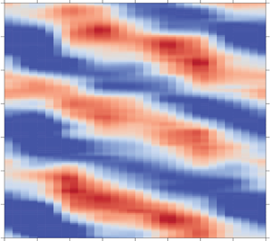The structure of the BZF can be seen well in figure 4(c), where the temperature (colour code) measured at $z=H/2$ is plotted as a function of the azimuthal position ($x$-axis) and time ($y$-axis). The time span plotted here corresponds to approximately 8 min. Albeit the spatial resolution is significantly smaller than in the simulation (figure 4b), one clearly sees the signature of the BZF, namely a mode $k=1$ wave with warm temperature on one side of the cell and cold temperature on the opposite side. In particular, we see here that the temperature structure drifts in the azimuthal direction with negative drift rate $\partial \theta _m/\partial t <0$, where $\theta _m$ is the azimuthal location of the warmest temperature, as defined below in (4.1).

Because the BZF in our $\varGamma =1/2$ cell has an azimuthal wavenumber of $k=1$, we can analyse it in the same way as large-scale circulation is usually analysed for the non-rotating (see e.g. Verzicco & Camussi Reference Verzicco and Camussi2003; Brown & Ahlers Reference Brown and Ahlers2007; Weiss & Ahlers Reference Weiss and Ahlers2011c) and rotating systems (Zhong & Ahlers Reference Zhong and Ahlers2010; Weiss & Ahlers Reference Weiss and Ahlers2011b). For this, we fit for every measurement in time a harmonic function

(4.1)\begin{equation} T_{i,j}=T_{w,j}+\delta_j\cos\left(\frac{i{\rm \pi}}{4}-\theta_j\right),\quad i=0,\ldots,7, \end{equation}

to the data. Here the index $i$ denotes the azimuthal position, and $j$ stands for the vertical position and takes indices $j=(\text {`}b\text {'}, \text {`}m\text {'}, \text {`}t\text {'})$, corresponding to the vertical locations $z=(H/4, H/2, 3H/4)$. The fit parameters are the azimuthally averaged wall temperature $T_{w,j}$, the amplitude $\delta _j$ and the orientation $\theta _j$. An example of the data and the corresponding fit is shown in figure 4(d). Note that this approach works for both analysing the LSC for small rotation rates as well as analysing the BZF for larger rotation rates. In the following, we will only focus on the dynamics of the azimuthal orientations $\theta _{j}$. The average temperature $T_{w,j}$ will be discussed later in § 5. The amplitudes $\delta _{j}$ are well reflected in measurements of $d$ (see § 6.1) and $\sigma$ (see § 6.2) and therefore will also not be discussed now.

4.1. The azimuthal drift of the BZF

Figure 5(a) shows the evolution of $\theta _{m}$ (at midheight) as a function of time. Here, we have made $\theta _{m}$ continuous by adding or subtracting $2{\rm \pi}$ whenever the difference $\theta _m(t_{i+1})-\theta _m(t_{i})$ at consecutive time steps was larger than ${\rm \pi}$ or smaller than $-{\rm \pi}$, respectively. The data plotted in this way show a nearly linear change of $\theta _m$ with time, indicating a monotonic drift with fairly constant drift speed $\omega _m=\langle \partial \theta _m/\partial t\rangle _t$.

Figure 5. (a) Azimuthal orientation of the LSC (for small 1/Ro) and the BZF (for large 1/Ro) as a function of time for ${\textit {Ra}}=4.9\times 10^{13}$ (run E2e) and various 1/Ro. (b) The average azimuthal drift velocity $\omega _{t,m,b}/\varOmega$ for heights $z/H=0.75$ (blue circles), $z/H=0.5$ (green diamonds) and $z/H=0.25$ (red squares). (c) The average azimuthal drift velocity $\omega _m/\varOmega$ as a function of 1/Ro and for various Ra (see legend). Horizontal dashed lines mark $\omega _m/\varOmega =0$. The vertical dashed lines mark $1/{\textit {Ro}}^*_1$ and $1/{\textit {Ro}}^*_2$. (d) Same data as in (c) multiplied by $-1$, only shown for $1/{\textit {Ro}}>1$ and plotted in a double-logarithmic plot. The black lines mark power laws with exponents $-3/4$ and $-5/3$ for comparison.

We already see here that the average drift velocity is a non-monotonic function of 1/Ro. Even the direction of rotation changes with increasing 1/Ro. For very small 1/Ro $\omega _m$ is positive, which means that the observed structure rotates in the same direction (in the rotating frame) as the convection cell, i.e. in the prograde or cyclonic direction. The value of $\theta _m$ decreases with time for large 1/Ro, which suggest a retrograde or anticyclonic motion of the temperature structure in the region close to the sidewall. This anticyclonic movement of the temperature field corresponds to the reported drift of the BZF in Zhang et al. (Reference Zhang, van Gils, Horn, Wedi, Zwirner, Ahlers, Ecke, Weiss, Bodenschatz and Shishkina2020).

For a more quantitative analysis we calculate the average drift speed $\omega _{(b,m,t)}$ as the slope of a linear fit to $\theta _{(b,m,t)}$. The result is plotted in figure 5(b). We see that, for sufficiently small rotation rates ($1/{\textit {Ro}}<1/{\textit {Ro}}^*_1$), there is a discrepancy between the drift rates measured at heights $H/4$, $H/2$ and $3H/4$. While $\omega _b$ and $\omega _t$ are almost zero, we see a finite drift of the structure in positive (cyclonic) direction at the middle, i.e. $\omega _m >0$. With increasing 1/Ro also $\omega _m$ increases and reaches a maximum at around $1/{\textit {Ro}}\approx 0.3$ or so, before it decreases again and reaches zero at $1/{\textit {Ro}}\approx 1/{\textit {Ro}}^*_1$. We note that differences in the drift rates at the top and bottom compared to the midheight were also observed in measurements in a $\varGamma =1/2$ cell with water ($Pr=4.38$) as the working fluid (Weiss & Ahlers Reference Weiss and Ahlers2011b). There, however, a prograde rotation was observed at all three heights for slow rotation that turned into a retrograde rotation for faster rotation rates.

What is measured for such small 1/Ro is not the BZF, but the structure of the LSC, which is not a coherent structure close to the sidewall. Consider a large-scale circulation roll of elliptical shape that lies diagonally inside the convection cell. Then, the fluid flows at midheight on average towards the cell centre, and the Coriolis force causes an acceleration of the azimuthal velocity, causing a cyclonic drift at midheight but no or only a very slow drift at $H/4$ and $3H/4$. The shape and strength of the LSC is clearly a function or Pr and hence quantitative differences are expected for different Pr.

For $1/{\textit {Ro}}>1/{\textit {Ro}}_1^*$ the drifts $\omega _{j}$ are the same for all heights and negative, i.e. in anticyclonic direction, suggesting a vertical coherent temperature structure – the BZF. With increasing rotation rate $\omega _{j}$ decreases as well and reaches a minimum at $1/{\textit {Ro}}\approx 6$. A further increase in $1/{\textit {Ro}}$ results again in an increase of $\omega _j$, so it reaches zero asymptotically.

We will now compare the effect of Ra on this observation. Therefore, we show in figure 5(c) $\omega _m$, normalised with the rotation velocity of the convection cylinder $\varOmega$ for different Ra as a function of 1/Ro. First of all, we see that data for different Ra collapse very well for large 1/Ro, but not so much for small 1/Ro. That is an initial cyclonic drift ($\omega _m/\varOmega >0$) for small 1/Ro turns into an anticyclonic drift $\omega _m/\varOmega < 0$ for large 1/Ro. The 1/Ro where $\omega _m/\varOmega =0$ is, albeit close to $1/{\textit {Ro}}^*_1$, smaller for larger Ra. A similar Ra-dependency has also been observed in previous experiments with water ($Pr=4.38$) (Weiss & Ahlers Reference Weiss and Ahlers2011b). For larger 1/Ro, $\omega _m/\varOmega$ reaches again a minimum and then increases asymptotically to zero.

The collapse of different Ra-data for sufficiently large 1/Ro occurs when the BZF is present, which suggests that the drift rate of the BZF ($\omega _m$) is for a given 1/Ro proportional to $\varOmega$ (or 1/Ek), but otherwise independent of Ra. We only cover nearly a decade in 1/Ro, and therefore it is difficult to compare our data with scaling laws observed or predicted by others. Nevertheless, we show in figure 5(d) the same data again ($-\omega /\varOmega$) for large 1/Ro plotted in a double-log plot. In this logarithmic representation of $-\omega /\varOmega$, small dependencies of Ra become visible at the largest 1/Ro. We note, however, that also Pr varies slightly and hence it is unclear whether the variations in $\omega /\varOmega$ are caused by Ra or Pr.

In this representation, no single scaling over the entire shown 1/Ro-range is visible. For $2\lesssim 1/{\textit {Ro}}\lesssim 7$ the data seem to follow $\propto (1/{\textit {Ro}})^{-3/4}$ or so. For larger 1/Ro data for different Ra seem to diverge slightly and show a larger negative exponent. We note that Zhang et al. (Reference Zhang, Ecke and Shishkina2021) observed a normalised BZF drift rate of $\omega /\varOmega \propto 1/{\textit {Ro}}^{-5/3}$, which is not too far from the small-Ra data at larger 1/Ro. We further note that in a recent measurement in slender cylinders ($\varGamma =0.2$) at ${\textit {Pr}}=5.2$ (de Wit et al. Reference de Wit, Guzmán, Madonia, Cheng, Clercx and Kunnen2020) a relation $\omega _{sc}H^2/\nu = 6 \times {\textit {Ra}}^{1.16}$ was measured, however, at constant ${\textit {Ek}}=10^{-7}$. We cannot compare our data with their results, since their dependency on Ek is unknown. We note, however, that a relation $\omega _{sc}H^2/\nu \propto {\textit {Ek}}^{3.32}{\textit {Ra}}^{1.16}$ would remove the Ra-dependency when plotted as a function of 1/Ro. This in turn would then lead to $\omega /\varOmega \propto (1/{\textit {Ro}})^{-2.32}$, which is rather different to our data.

4.2. The azimuthal Fourier modes of the BZF

Fitting (4.1) to the thermistor measurements as described above also gives the amplitudes $\delta _{j}$, which we have not discussed so far. By fitting (4.1) to the 8 sidewall thermistors, we gain with $\delta _j$ basically the energy in the first Fourier mode ($E_1$). However, since we measure the temperature at 8 azimuthal positions, we can also calculate the energy of the second, third and fourth, Fourier modes, namely $E_2$, $E_3$ and $E_4$.

Figure 6 shows the time average of the first four Fourier modes normalised with the total spectral energy $E_{tot}=\sum ^4_{n=1}E_n$ as a function of 1/Ro for ${\textit {Ra}}=2\times 10^{11}$ (a) and ${\textit {Ra}}=8\times 10^{14}$ (b). Up to a rotation rate of $1/{\textit {Ro}}\approx 1/{\textit {Ro}}^*_2$ the first mode $E_1$ is significantly larger than the others. This is due to the existence of the LSC for small 1/Ro and due to the BZF at larger 1/Ro. However, it is interesting that $E_1/E_{tot}$ reaches a local maximum pretty much at $1/{\textit {Ro}}^*_1$. After that, it decreases slightly first, before it increases again with increasing 1/Ro. In experiments with water in a cell of $\varGamma =0.5$ we have seen similarly a maximum at $1/{\textit {Ro}}\approx 0.8$ of $E_1/E_{tot}$ (see figure 4a in Weiss & Ahlers Reference Weiss and Ahlers2011b).

Figure 6. Azimuthal Fourier energy of the temperature measured at $z/H=0.5$ for ${\textit {Ra}}=2\times 10^{11}$ (a) and ${\textit {Ra}}=8\times 10^{14}$ (b). Horizontal dashed lines mark $1/{\textit {Ro}}^*_1$ and $1/{\textit {Ro}}^*_2$.

We can only speculate, but it seems that $E_1$ is enhanced right when the BZF starts to appear and the LSC vanishes. The fact that we see the same feature for very different Ra and Pr suggests that the transition of the LSC into the BZF only depends on 1/Ro. For larger 1/Ro, say $1/{\textit {Ro}}>1/{\textit {Ro}}_2^*$, the first mode $E_1/E_{tot}$ decreases for small ${\textit {Ra}}=2\times 10^{11}$, while for ${\textit {Ra}}= 8\times 10^{14}$ it continues to increase. This is in accordance with the behaviour of the standard deviation $\sigma$ shown in figure 15. This finding is a bit puzzling. While the decreases of $E_1/E_{tot}$ suggests that the BZF only exists in a finite 1/Ro-range, which depends on Ra, we in fact know from simulation (Zhang et al. Reference Zhang, van Gils, Horn, Wedi, Zwirner, Ahlers, Ecke, Weiss, Bodenschatz and Shishkina2020) that the size of the BZF layer $\delta _{BZF}$ is expected to slightly decrease with Ra at a fixed 1/Ro following $\delta _{BZF}\propto {\textit {Ra}}^{-0.08}{\textit {Ro}}^{0.66}$. Since it seems reasonable to believe that the pumping efficiency inside the BZF decreases with decreasing thickness $\delta _{BZF}$ one would expect the decrease of $E_1/E_{tot}$ to appear at smaller 1/Ro for the larger Ra, i.e. the opposite to what is observed in the measurements.

5. Mean temperature profiles

As shown in figure 1, 62 thermistors were installed inside the cell, predominantly close to the sidewall, to acquire vertical temperature profiles. We now want to analyse these data and see how the vertical temperature profiles as well as fluctuations change as a function of 1/Ro. We note that the thermal and viscous boundary layers close to the top and bottom plates are only of the order of a millimetre or less and are not resolved in these measurements. Data presented here thus are measurements in the (vertical) bulk region.

Before we discuss the effect of rotation on the vertical temperature profiles, we quickly recapitulate what is known for the non-rotating case. It has been shown by Ahlers et al. (Reference Ahlers, Bodenschatz, Funfschilling, Grossmann, He, Lohse, Stevens and Verzicco2012a) and Ahlers, Bodenschatz & He (Reference Ahlers, Bodenschatz and He2014) that the vertical temperature profile close to the sidewall can be well approximated by a logarithmic function of the form

(5.1)\begin{gather} \varTheta(z) ={-}a_b \ln\left(2z/H\right)+b_b \quad \text{for}\ z < H/2, \end{gather}

(5.2)\begin{gather}\varTheta(z) = a_t \ln\left(1-2z/H\right)+b_t \quad \text{for}\ z>H/2, \end{gather}

where $\varTheta (z)$ denotes the normalised temperature

(5.3)\begin{equation} \varTheta = \frac{\langle T \rangle -T_m}{\Delta T}, \end{equation}

with $\langle \cdots \rangle$ denoting the time average over an entire run.

The logarithmic slope of the temperature profiles, i.e. the coefficients $a_{t,b}$, decrease with Ra following a power law of $a_{t,b}\propto {\textit {Ra}}^{-\eta }$, where $\eta$ depends on the radial position. Our measurements were conducted with the same cell that was used for the comprehensive investigation of the vertical temperature profile (Ahlers et al. Reference Ahlers, Bodenschatz and He2014) and our measurements for the non-rotating case are in accordance with those reported in Ahlers et al. (Reference Ahlers, Bodenschatz and He2014).

Figure 7 shows $\varTheta$ as a function of $z$ very close to the sidewall at radial distance $r=0.98R$, for ${\textit {Ra}}=4.9\times 10^{13}$ and different 1/Ro. While the solid lines in figure 7(a) are just guides to the eyes, we show the same data in figure 7(b) plotted against a logarithmically scaled $x$-axis, and see that the data indeed follow straight lines for all rotation rates. This indicates that, also under rotation, the vertical temperature profiles are well represented by a logarithmic function ((5.1) and (5.2)) over the measured vertical distance, which is approximately a single order of magnitude. Furthermore, we see that the profiles at the bottom and the top behave rather similarly, at least for the Ra plotted here. The logarithmic temperature gradient increases with increasing rotation, which also suggests that the temperature drop across the thin top and bottom boundary layers is reduced with increasing rotation rate, an observations that is in accordance with previous findings, such as, for instance, those by Julien et al. (Reference Julien, Rubio, Grooms and Knobloch2012b). The steeper temperature gradient in the bulk is a result of suppressed vertical fluid motion due to Coriolis forces. We also see that the temperature at midheight is close to the mean temperature $T_m$ between top and bottom plates. This is because non-OB effects are rather small in this particular case as the temperature difference between bottom and top was only $\Delta T=5\ \textrm {K}$ and the pressure was not too high (10 bar – run E2e). We note that non-OB effects in pressurised gases are expected to lower the midheight temperature compared to $T_m$. The very same effect would occur under the presence of centrifugal forces, which apparently also do not play a significant role here.

Figure 7. (a) Reduced temperature $\varTheta$ as a function of the vertical distance from the bottom plate for ${\textit {Ra}}=4.9\times 10^{13}$ and various 1/Ro (see legend) and at radial position ${\rm r/R} =0.98$. (b) The same data plotted against $z/H$ (bottom $x$-axis) and against $1-z/H$ (top $x$-axis). The top and bottom $x$-axes are both logarithmically scaled. In this way we can compare measurements from the bottom half of the cell with measurements from the top half of the cell. The solid lines in (a,b) are logarithmic fits of ((5.1) and (5.2)) to the data. The vertical dotted line marks $z=H/2$.

Figure 8 shows the logarithmic slope $a_b$ as a function of 1/Ro for data taken at $r/R=0.98$. We have seen already in figure 7 that, with increasing rotation, the coefficient $a_t$ ($a_b$) increases. In figure 8(a), we see that the change of the logarithmic slope $a$ with 1/Ro is not the same for all 1/Ro. Instead, $a$ for small 1/Ro remains rather constant, but increases for larger 1/Ro. The transition between these two regimes coincides approximately with $1/{\textit {Ro}}^{*}_{1}$. The increase of $a_t$ ($a_b$) is well approximated for large 1/Ro by a power law $a_{t,b}\propto 1/{\textit {Ro}}^{\varepsilon }$, with exponents $\varepsilon =0.51\pm 0.02$ and $0.50\pm 0.02$ for both top and bottom halves of the cell, respectively. The fact that this exponent resembles a pitchfork bifurcation is merely a coincidence for the particular case of ${\textit {Ra}}=4.9\times 10^{13}$. We will see below that the exponent actually depends on Ra.

Figure 8. (a) Log slope for the top $a_t$ and the bottom $a_b$ as a function of 1/Ro for ${\textit {Ra}}=4.9\times 10^{13}$ for measurements close to the sidewall at $r/R=0.98$. Dotted vertical lines mark $1/{\textit {Ro}}^{*}_{1}$ and $1/{\textit {Ro}}^{*}_{2}$. Fitted dotted lines show $a_{t}\sim 1/{\textit {Ro}}^{0.51}$, $a_{b}\sim 1/{\textit {Ro}}^{0.50}$ for $1/{\textit {Ro}}>1/{\textit {Ro}}^{*}_1=0.8$. (b) Fit parameters $b_t$ and $-b_b$ as a function of 1/Ro for the bottom (red squares) and the top (blue bullets) part of the cell in log–log representation. The error bars mark the uncertainty of the fit value.

In figure 8(b) we show how the offset parameters $b_t$ and $b_b$ change with increasing 1/Ro. From (5.1) and (5.2) we see that $b_{t,b}$ give us the fitted temperature at midheight ($z=H/2$). Since in the ideal OB case it is $\theta (H/2)=0$, the $b_{t,b}$ mark whether the fits overshoots or undershoots this value, and hence also contain information on the relative slope of the temperature profile at the top and the bottom compared to the temperature gradient at midheight. For the ideal OB case, we expect $b_b$ and $b_t$ to have opposite signs. For a better comparison, we thus plot in figure 8(b) $b_t$ and $-b_b$ as functions of $1/{\textit {Ro}}$.

We see that $b_t$ is positive and $b_b$ is negative for all 1/Ro, denoting that the logarithmic fits undershoot slightly the temperature at $z=H/2$. Furthermore, we see that there is an asymmetry between the bottom and the top. For small 1/Ro $b_t$ is considerably smaller than $b_b$. This discrepancy might be due to small non-OB effects, or imperfections in the experimental set-up that destroy the up–down symmetry of the system. While $b_t$ is rather constant for $1/{\textit {Ro}}<1/{\textit {Ro}}^{*}_{1}$, it increases for $1/{\textit {Ro}}>1/{\textit {Ro}}^{*}_{1}$. This trend is also visible for $b_b$, albeit much weaker.

In general, the fit of (5.1) and (5.2) to the data returns small residuals for not too large rotation rates, i.e. $1/{\textit {Ro}} \lesssim 8$. For larger 1/Ro the vertical temperature profile starts to deviate from a logarithmic profile consistently, as shown in figure 8(b). We further note that the residuals are in general larger at the cold top part of the cell than in the warm lower part. However, for sufficiently fast rotation ($1/{\textit {Ro}} \lesssim 1/{\textit {Ro}}\approx 8$), the residuals at both locations merge and increase consistently.

To compare measurements at different Ra, we show in figure 9(a) the logarithmic slopes normalised with their corresponding values without rotation (i.e. $a_t(1/{\textit {Ro}})/a_t(0)$) as a function of the rotation rate $1/{\textit {Ro}}$. In this way, we can compare the change of the vertical profile for different Ra. We see in this log–log representation that the onset of the $a_t$ enhancement occurs at around $1/{\textit {Ro}}^{*}_{1}$ for all Ra. The increase of $a_t$ for $1/{\textit {Ro}} > 1/{\textit {Ro}}^{*}_{1}$ is stronger for larger Ra. This comes as a surprise, since the change in Nu seems rather independent of Ra. Moreover, from figure 2, the Nu-reduction with Ra seems to be slightly smaller for larger Ra. We note in this context that the local effective heat conductivity is inversely proportional to the local vertical temperature gradient $\lambda _{eff} = q /(\Delta T/\Delta z)$. In particular, for larger Ra the slope increase can be well approximated using a power law with a Ra-dependent exponent of the form $a_t(1/{\textit {Ro}})/a_t(0) = K_a\times (1/{\textit {Ro}})^{\eta ({\textit {Ra}})}$, such that all data collapse. The fitted exponents $\eta$ are plotted as functions of Ra in the inset of figure 9(b) on a semi-logarithmic plot.

Figure 9. (a) Normalised logarithmic slope $a_t(1/{\textit {Ro}})/a_t(0)$ as a function of 1/Ro on a log–log plot for various Ra. The dashed straight lines are power law fits of the form $a_t/a_t(0)=0.0086\times (1/{\textit {Ro}})^{\eta (Ra)}$. Fits were done to the data points with $1/{\textit {Ro}} >3$. The vertical dashed lines mark $1/{\textit {Ro}}^{*}_{1}$ and $1/{\textit {Ro}}^{*}_{2}$. (b) The inset shows the fitted $\eta$ as a function of Ra on a semi-log plot. The black solid line is the function $0.031\ln (Ra)-0.46$, which represents the data decently well. With this, the data plotted in (a) collapse onto a single master curve in (b).

We note that, in this representation, the data for $\eta$ do not follow a straight line. In particular, the decrease of $\eta$ is stronger with decreasing Ra than a logarithmic function would suggest. However, as can be seen in figure 9(a), the normalised slopes deviate from the power law particularly strongly for small Ra and thus the uncertainty of $\eta$ is also large for these data points. However, a function $\eta = 0.031\ln (Ra)-0.45$ represents the data decently well (black line in the inset in figure 9b) and therefore all data $a_t/a_t(0)$ collapse onto a single master curve when plotted as a function of $(1/{\textit {Ro}})^{\eta ({\textit {Ra}})}$. At this point, these findings are purely empirical, but they hopefully can be used to compare with other measurements, DNS or theoretical models.

From measurements in the non-rotating system (Ahlers et al. Reference Ahlers, Bodenschatz and He2014) we know that the logarithmic slope of the vertical temperature profiles increases with increasing radial distance from the centre line $r/R$. This is not surprising, since at least for the non-rotating case vertical fluid motion and hence vertical fluid transport close to the sidewall are reduced. In figure 10(a) we show how $a_b$ changes with 1/Ro at different $r/R$. For small rotation rates ($1/{\textit {Ro}}<1/{\textit {Ro}}^*_1$), similar to the non-rotating case, the $a_b$ measured closest to the radial centre ($r/R=0.73$) have the smallest values and increase with radial distance. It is interesting, however, that $a_b$ in this regime is not affected by a change of 1/Ro for $r/R=0.98$ and $r/R=0.96$, very little for $r/R=0.93$ but it changes increasingly for $r/R=0.73$. As a result, the $a_b$ for different radial distances are getting closer to each other with increasing 1/Ro and finally, somewhere before $1/{\textit {Ro}}^{*}_{2}$, collapse on a single power law curve of the form $a_b\propto (1/{\textit {Ro}})^{0.63}$ (for ${\textit {Ra}}=4.9\times 10^{13}$), so that $a_b$ is independent of the radial location.

Figure 10. (a) Change of $a_b$ as a function of $1/{\textit {Ro}}$ for four different radial locations and ${\textit {Ra}}=4.9\times 10^{13}$. The black dashed line is a fit of a power law $a_t\propto 1/{\textit {Ro}}^{\varepsilon }$ to all data for $1/{\textit {Ro}}>3$, resulting in $\epsilon =0.63$. Thin dotted vertical lines show $1/{\textit {Ro}}^{*}_{1}$ and $1/{\textit {Ro}}^{*}_{2}$. (b) The offset $b_b$ as a function of 1/Ro for different radial positions. Symbols are as in (a).

A similar behaviour is observed for the offset $b_b$ shown in figure 10(b). Although the data are more scattered, the values for different $r/R$ differ for $1/{\textit {Ro}}<1/{\textit {Ro}}_1^*$, but are getting closer for larger 1/Ro. This behaviour suggests that a radial symmetry, which is broken by the LSC in the non-rotating case, is gradually being restored in the rotating case. This is quite surprising. As we will discuss in the next section, close to the wall ($r/R=0.98$, 0.96 and 0.93) the temperature and velocity fields are dominated by the BZF and one would expect to see a different average temperature field there and in the radial bulk ($r/R=0.73$). It might be that, due to Coriolis forces under rotation, mixing in the horizontal direction is much more effective and thus faster compared to the vertical transport of warm and cold fluid, or in other words, the eddy diffusion time scales in the vertical direction are much smaller than those in horizontal direction. Therefore, vertical temperature gradients increase and horizontal temperature gradients must decrease with increasing rotation rates. Thus, even though the temperature and flow fields are different in the BZF and the radial bulk, the time-averaged temperatures are surprisingly similar.

6. Temperature fluctuations

6.1. The full PDF of the temperature fluctuations

So far, we have looked at the time-averaged temperature at different positions as a function of Ra and 1/Ro. In this section, we want to look at temperature fluctuations, as they provide valuable information about the flow field and the specific heat transport mechanisms. Therefore, we first consider the full PDF of the normalised temperature $\tilde {T}=(T-T_m)/\Delta T$ and will discuss some of its quantities later.

Figure 11 shows the temperature PDFs $p(\tilde T)$ for heights $z/H=0.287$ (bottom), 0.493 (midheight) and 0.75 (top) and four different rotation rates, measured close to the sidewall at $r/R=0.98$. For the non-rotating case the distribution is symmetric for the midheight (green diamonds) with slightly larger tails than what would be expected for a Gaussian distribution. The distributions for the temperature at the bottom and the top are skewed in the way that at the bottom (top) warmer (colder) temperatures are measured more often than for a Gaussian distribution. The deviation from the Gaussian originates from the warm (cold) plumes that are rising (falling), which are not well mixed with the turbulent fluid. In fact, it has been suggested by Wang, He & Tong (Reference Wang, He and Tong2019) that temperature distributions close to the top and bottom plates can be represented by a superposition of a Gaussian, which reflects fluctuations in the well-mixed turbulent bulk, and an exponential distribution, which represents the contribution from thermal plumes. While we refrain from a detailed analysis of our temperature measurements, we note that the distributions for the non-rotating case are qualitatively consistent with such a superposition.

Figure 11. Probability densities of the temperature $p(\tilde {T})$ measured at ${\textit {Ra}}=4.9\times 10^{13}$ and radial location $r/R=0.98$. Different symbols mark the different heights $z/H=0.287$ (red squares), $z/H=0.493$ (green diamonds) and $z/H=0.75$ (blue bullets). The different panels are for inverse Rossby numbers $1/{\textit {Ro}}=0$ (a), $1/{\textit {Ro}}=0.74$ (b), $1/{\textit {Ro}}=3.06$ (c) and $1/{\textit {Ro}}=7.37$ (d). The solid lines in (a,b) represent single Gaussian fits. The solid lines in (c,d) represent fits of bimodal Gaussians (6.1) to the data.

The temperature distribution clearly changes with increasing rotation rate, not just in quantitative, but also in qualitative terms. At very slow rotation rates, $p(\tilde T)$ actually becomes less skewed and follows more a Gaussian distribution, as shown in figure 11(b). This suggests that warm and cold plumes mix faster with the background fluid under very slow rotation. Very warm and very cold plumes lose their heat faster under faster rotation when they move from the bottom and top plates towards the thermistor positions at $H/4$ and $3H/4$.

At faster rotation rates, the standard deviation increases as the maximum of the distribution widens. At sufficiently fast rotation, in $p(\tilde {T})$ the peak splits into two peaks denoting a bimodal temperature distribution (figure 11c). The two peaks move apart from each other with increasing 1/Ro, see figure 11(d). We have already reported on this observation in a previous publication, in which we explain this bimodal PDF as the signature of the BZF that transports warm fluid from the bottom to the top close to the sidewall at one side and cold fluid to the bottom at the opposite side, thus preventing effective mixing between them (Zhang et al. Reference Zhang, van Gils, Horn, Wedi, Zwirner, Ahlers, Ecke, Weiss, Bodenschatz and Shishkina2020).

For a quantitative analysis we fit a superposition of two Gaussian functions of the form

(6.1)\begin{equation} p(\tilde{T})=\frac{A}{\sqrt{2{\rm \pi}\sigma_{1}^{2}}}\exp\left(-\frac{(\tilde{T}-\mu_1)^2}{2\sigma_{1}^{2}}\right)+\frac{1-A}{\sqrt{2{\rm \pi}\sigma_{2}^{2}}}\exp\left(-\frac{(\tilde{T}-\mu_2)^2}{2\sigma_{2}^{2}}\right) ,\end{equation}

to the data. Equation (6.1) has five independent parameters, the means $\mu _i$, the standard deviations $\sigma _i$ ($i=1,2$) and a parameter $A\leq 1$, which determines the relative ratio of the amplitudes of the two peaks. From now on we follow the convention that the index $1$ refers to the colder mode, such that it is always $\mu _1 <\mu _2$.

By fitting (6.1) to the data, we can describe the PDF by the parameters $A$, $\mu _i$ and $\sigma _i$ and we can investigate how these parameters change with increasing rotation rates.

We show in figure 12(a) $\mu _1$ and $\mu _2$ as functions of 1/Ro at different vertical positions. We see that for small rotation rates ($1/{\textit {Ro}}\lesssim 1/{\textit {Ro}}^*_1$) all $\mu _{1,2}$ are nearly independent of 1/Ro and $\mu _1$ (open symbols) is for any height rather close to $\mu _2$ (closed symbols). In particular, for measurements at midheight, the data points are on top of each other, indicating that no bimodal Gaussian is present. As we have mentioned above, the temperature PDFs measured at the top and the bottom half of the cell are skewed. This skewness is detected when fitting (6.2) to the data and hence we get slightly different values for $\mu _1$ and $\mu _2$. This is not the case for measurements at midheight, where warm and cold plumes are sufficiently mixed. In the regime of small rotation rates, it even seems as if the difference between $\mu _1$ and $\mu _2$ decreases slightly for the top and bottom parts with increasing 1/Ro.

Figure 12. (a) Fitted expectation values $\mu _1$ (open symbols) and $\mu _2$ (closed symbols) for vertical locations $z/H=0.287$ (red squares), $z/H=0.493$ (green diamonds), $z/H=0.75$ (blue circles) as functions of 1/Ro. (b) Relative distance of the two peaks $d$ as defined in (6.2). Vertical dashed lines mark $1/{\textit {Ro}}^*_1$ and $1/{\textit {Ro}}^*_2$. Data were acquired at ${\textit {Ra}}=4.9\times 10^{13}$ (E2e) and at radial position $r/R=0.98$.

When the rotation rates exceed $1/{\textit {Ro}}^*_1$, for the measurements at midheight, two clearly distinguishable peaks occur, (i.e. a bimodal distribution) resulting in a decreasing $\mu _1$ and an increasing $\mu _2$. For measurements at the top and bottom, however, only one of the $\mu _{1,2}$ changes in this regime. These are a decrease of $\mu _1$ for the cold top and an increase of $\mu _{2}$ for the warm bottom. This observation is quite significant. It suggests that, for example, at the bottom, the pumping of warm fluid from the bottom inside the BZF starts to play a role, while mixing is still small so that the cold flow from the top is not being heated up very strongly. In fact, in this regime, the red open squares ($\mu _1$ at the top) and the blue solid circles ($\mu _2$ at the bottom) approach each other, meaning that the cold areas at the bottom become a bit colder while the warm areas at the top become a bit warmer due to the relative strong pumping inside the BZF.

This changes at $1/{\textit {Ro}}^*_2$. Now the warm fluid at the top part ($\mu _2$ – blue solid circles) also cools down and the cold fluid at the bottom ($\mu _1$ – red open squares) heats up. While there is still a vertical transport of fluid inside the BZF, the size of the BZF decreases with increasing rotation rate (see Zhang et al. Reference Zhang, van Gils, Horn, Wedi, Zwirner, Ahlers, Ecke, Weiss, Bodenschatz and Shishkina2020). Therefore the cold down (warm up) flow inside the BZF gets heated (cooled) from the bulk, where the temperature gradient increases. This observation is in accordance with the temperature gradient measurements presented in figure 10(a). There, the gradients in the bulk and close to the sidewall, i.e. in the BZF converge for rotation rates $1/{\textit {Ro}}^*_1 < 1/{\textit {Ro}} < 1/{\textit {Ro}}^*_2$.

It is also insightful to plot the temperature difference between the warm and the cold areas in the BZF. For this, we look at the relative distance between the two peaks as suggested in Holzmann & Vollmer (Reference Holzmann and Vollmer2008)

(6.2)\begin{equation} d=\frac{|\mu_1-\mu_2|}{2\sqrt{\sigma_1\sigma_2}}. \end{equation}

We note that $d$ tells us something about how well (small $d$) or badly (large $d$) warm and cold fluid is mixed. We plot in figure 12(b) $d$ as a function of 1/Ro for measurements at the top, the middle and the bottom parts of the cell. In this representation, we see, in particular for the midheight of the cell (green diamonds), a bifurcation-like behaviour of $d$ at $1/{\textit {Ro}}\approx 1/{\textit {Ro}}^*_1$, which we interpret as the onset of the BZF. The PDF consists only of a single peak for smaller 1/Ro – thus $d\approx 0$ – and at $1/{\textit {Ro}}^*_1$ the PDF splits into a bimodal distribution, with warm fluid being pumped inside the BZF from the bottom to the top and cold fluid being pumped from the top to the bottom, causing $d$ to sharply increase. The increase of $d$ continues for larger 1/Ro. This implies that, in this regime, the lateral mixing is small compared to the heat transport by vertical pumping from the top and bottom. For the largest 1/Ro, however, we see a decrease of $d$ for just a single point, which we believe is real and not just an outlier. We know (Zhang et al. Reference Zhang, van Gils, Horn, Wedi, Zwirner, Ahlers, Ecke, Weiss, Bodenschatz and Shishkina2020) that the width of the BZF layer shrinks with $\propto (1/{\textit {Ro}})^{-0.66}$ and thus thermal diffusion starts to thermally couple the bulk with the BZF, which is expected to lead to a reduced $d$ at sufficiently large rotation rates.

The behaviour of $d$ for the top (blue circles) and bottom (red squares) is for small 1/Ro qualitatively similar and for larger 1/Ro also quantitatively similar. Just as we discussed above, for small rotation rates ($1/{\textit {Ro}} < 1/{\textit {Ro}}^*_1$) at heights $H/4$ and $3H/4$, $d$ is finite due to the skewness of the PDF. This fact is captured when naively fitting two Gaussian (i.e. (6.1)) to the PDF.

The qualitative changes of $p(\tilde T)$ are restricted to a thin region close to the sidewall (the BZF). This is shown in figure 13, where $p(\tilde {T})$ is plotted as measured at $r/R=0.98$ (a) and at $r/R=0.73$ (b) for different 1/Ro and at midheight of the cell. We see that the change from a uni-modal to a bimodal distribution with increasing 1/Ro is clearly seen at $r/R=0.98$, but not for $r/R=0.73$. There, $p(\tilde {T})$ seems to be unaffected by rotation in the observed 1/Ro-range. Up to large 1/Ro $p(\tilde {T})$ follows a stretched exponential, which is in accordance with previous findings for the temperature fluctuations in the bulk (e.g. Castaing et al. Reference Castaing, Gunaratne, Heslot, Kadanoff, Libchaber, Thomae, Wu, Zaleski and Zanetti1989; Ching Reference Ching1991; Niemela et al. Reference Niemela, Skrbek, Sreenivasan and Donnelly2000). An exponential fit of the function $e^{-c|x|^{\beta }}$ yields $\beta =1.34\pm 0.03$, i.e. the decrease is somewhere in between an exponential ($\beta =1$) and a Gaussian ($\beta =2$).

Figure 13. Probability density distribution of the reduced temperature $(T-T_m)/\Delta T$ at height $z/H=0.49$ and ${\textit {Ra}}=4.9\times 10^{13}$ (run E2e) for radial distances from the centre line $r/R=0.98$ (a) and $r/R=0.73$ (b) and for three different 1/Ro.

It is somehow unfortunate that we cannot resolve the BZF sufficiently well in space and therefore cannot plot a detailed radial profile of it, e.g. $d(r/R)$. We nevertheless plot in figure 14 data points $d$ for the four available thermistors for different 1/Ro (solid symbols) and add estimates for the width of the BZF ($\delta _{BZF}$) from numerical simulations (Zhang et al. Reference Zhang, van Gils, Horn, Wedi, Zwirner, Ahlers, Ecke, Weiss, Bodenschatz and Shishkina2020, Reference Zhang, Ecke and Shishkina2021) as open symbols. These estimates are $\delta _{BZF} = 3.55\times {\textit {Ra}}^{-0.08}\times (1/{\textit {Ro}})^{-0.66}$. The dashed lines in figure 14 are convenient functions as a guide to the eye to better illustrate the estimated radial profile of $d$. We note that the $\delta _{BZF}$ are in accordance with our observation.

Figure 14. Peak-to-peak distance at midheight $d$ as defined in (6.2) as a function of the radial position. Filled symbols are data measured for ${\textit {Ra}}=4.9\times 10^{13}$. Open symbols show estimates for the width of the BZF $\delta _{BZF}$ according to Zhang et al. (Reference Zhang, van Gils, Horn, Wedi, Zwirner, Ahlers, Ecke, Weiss, Bodenschatz and Shishkina2020). Dashed lines are guides to the eyes.

6.2. Amplitude of temperature fluctuations

Above, we have already analysed average temperatures (§ 5) and the locations of the peak of the PDF. Now, we want to look at the standard deviations of the temperature, defined as

(6.3)\begin{equation} \sigma(z,r)=\frac{\sqrt{\langle\left[T(t,z,r)-\langle T(t,z,r)\rangle_t\right]^2}\rangle_t}{\Delta T}. \end{equation}

Here, $\langle \dots \rangle _t$ denotes the average over time. Please note that in this way we have already normalised the temperature fluctuations by the temperature difference $\Delta T$.

Before we discuss the rotating case, let us again quickly recapitulate what is known for the non-rotating case.

At a given position and for sufficiently large Ra, $\sigma$ decreases with increasing Ra, according to $\sigma \propto {\textit {Ra}}^{-\alpha }$, as has been observed e.g. by Castaing et al. (Reference Castaing, Gunaratne, Heslot, Kadanoff, Libchaber, Thomae, Wu, Zaleski and Zanetti1989), Niemela et al. (Reference Niemela, Skrbek, Sreenivasan and Donnelly2000), Daya & Ecke (Reference Daya and Ecke2002) and Grossmann & Lohse (Reference Grossmann and Lohse2004). This decrease is due to stronger mixing as the turbulence intensity increases. The exponent $\alpha$ does slightly depend on the radial position in the flow. In fact we measure $\alpha =0.101$ for $r/R=0.73$ and $\alpha =0.084$ for $r/R=0.98$ for measurements at midheight ($z=H/2$). These values are comparable with other values found in the literature.

Furthermore, the temperature fluctuations depend strongly on the vertical coordinate and are largest when measured close to the top and bottom plate and decrease towards the vertical centre. Similar to the time-averaged temperature, also the temperature fluctuations can be modelled as a logarithmic function of $z/H$, as reported by He et al. (Reference He, van Gils, Bodenschatz and Ahlers2014).

The data analysis in this subsection has so far dealt with temperature fluctuations and how they depend on Ra and their radial and vertical locations. We now want to focus on how the fluctuations are influenced by rotation.

For this we show in figure 15(a–c) temperature fluctuations at midheight of the cell at two different radial distances and for different Ra. Let us first focus on figure 15(a), where $\sigma$ is plotted as a function of 1/Ro, for different Ra. One sees that, at very small rotation, $\sigma$ is larger for smaller Ra, just as discussed above for the non-rotating case. For low rotations rates, $\sigma$ increases monotonically until it reaches a maximum, beyond which the temperature fluctuations decrease again with increasing $1/{\textit {Ro}}$. The rotation rate at which $\sigma$ reaches its maximum depends on Ra and is smallest for the smallest Ra; in our observed Ra range the maximum for the smallest Ra ($\approx 7.7\times 10^9$) is reached at $1/{\textit {Ro}}\approx 4$.

Figure 15. (a) Temperature fluctuations $\sigma$ as a function of $1/{\textit {Ro}}$ measured at $r/R=0.93$ and $z/H=0.493$ for different Ra (see legend). At this radial position, we expect the BZF to occur. (b) The same measurements normalised with the fluctuations without rotation $\sigma (1/{\textit {Ro}}=0)$. (c) Normalised fluctuations taken at midheight $z/H=0.493$ but at $r/R=0.73$, i.e. where no BZF is expected. (d) Normalised temperature fluctuations as a function of vertical coordinate at $r/R=0.98$, ${\textit {Ra}}=2.5\times 10^{13}$ and different 1/Ro (see legend) on a semi-log plot. Data were normalised with $\sigma _{0.5}=\sigma (z/H=0.5)$ for better visualisation. These measurements are for the bottom half of the cell. (e) Similar data for the fluctuations in the top half of the cell.

For a better comparison of the effect of Ra on $\sigma$ we normalised for each Ra $\sigma (1/{\textit {Ro}})$ by $\sigma (0)$ without rotation and plot the result in figure 15(b). We see that the data normalised in this way collapse rather well for $1/{\textit {Ro}} < 2$, but start to deviate for larger 1/Ro. In this normalised plot, one also sees that the relative increase in $\sigma$ is in fact larger for larger Ra. The data plotted here are acquired where the BZF occurs for sufficiently large 1/Ro ($\gtrsim 1/{\textit {Ro}}^*_1$). While for the non-rotating case larger Ra leads to a better mixing of warm and cold fluid, this fact is not very relevant inside the BZF, as it is less influenced by the turbulent flow in the radial bulk. In this regard, it is important to note that no sharp transition is observed in these plots. Instead, $\sigma$ increases rather smoothly until it reaches its maximum. This is all the more surprising since we have seen already in figure 12(b) that the distance between the maxima in the bimodal PDF increases quite abruptly at $1/{\textit {Ro}}^*_1$. One would guess that the distance between the peaks of the PDF $d$ contributes heavily to the measured temperature fluctuations. While this might nevertheless be the case, the plots here suggests that the PDF widens significantly before it splits into a bimodal distribution, i.e. before the BZF occurs.

For comparison, in figure 15(c) we also plot the normalised fluctuations as measured at $r/R=0.73$, outside the BZF in the radial bulk. The difference to the measurements in the BZF are clear, particularly for larger Ra. The fluctuations there are drastically reduced. Instead of a continuous increase with increasing 1/Ro, $\sigma /\sigma _0$ barely changes with 1/Ro up to $\approx 1/{\textit {Ro}}^*_1$, but then even decreases for the largest Ra with increasing 1/Ro. The Ra-dependency for larger $1/{\textit {Ro}}$ is reversed compared to what was observed at $r/R=0.93$. That is the smallest $\sigma /\sigma _0$ is for the largest Ra. For the smallest Ra, we still see a maximum close to $1/{\textit {Ro}}^*_2$, which even has very similar values of $\sigma /\sigma _0$ as measured for $r/R=0.93$. Why are measurements at $r/R=0.73$ and $r/R=0.93$ so different for large Ra but similar for small Ra? The answer is simple. The size of the BZF also depends on $\propto {\textit {Ra}}^\gamma$ with an exponent of $\gamma \approx -0.08$ according to Zhang et al. (Reference Zhang, Ecke and Shishkina2021). Based on this estimate, at $1/{\textit {Ro}}\approx 1/{\textit {Ro}}^*_2$ the BZF reaches for ${\textit {Ra}}=7.7\times 10^9$ still up to $r/R=0.71$ and the thermistor still measures the BZF. This is also the case for ${\textit {Ra}}=2.1\times 10^{10}$, where $1-\delta _{BZF}\approx 0.73r/R$. For the third smallest Ra, the thermistor at $r/R=0.73$ is outside but very close to where the BZF occurs, and one would expect the thermistor to still measure the thermal signature of the BZF, albeit with a smaller amplitude.

We see for ${\textit {Ra}}=8.4\times 10^{12}$ and ${\textit {Ra}}=4.9\times 10^{13}$ an increase of $\sigma /\sigma _0$ for $8<1/{\textit {Ro}}$, when measured at $r/R=0.73$. Further investigations are necessary to interpret this increase; however, it might be related to coherent vertical vortex structures, such as Ekman vortices in which warm and cold fluid is transported from the boundaries deep into the bulk areas.

After we have discussed fluctuations at midheight of the cell, we briefly want to discuss how the vertical temperature fluctuation profile changes with increasing rotation rate. In figure 15(d,e) we therefore plot the temperature fluctuations against a logarithmically scaled $z$-axis. Measurements were taken inside the BZF at $r/R=0.98$. The fluctuations are normalised with the fluctuations at midheight $\sigma _0$ to indicate the relative change as a function of the vertical position. Without rotation, fluctuations at the bottom and the top are significantly larger than the midheight fluctuations and, with increasing 1/Ro, the relative temperature fluctuations close to the top and bottom boundaries decrease, in other words the slope ${\partial (\sigma (z)/\sigma (0.5))}/{\partial z}$ decreases. Please recall that this is different to the logarithmic slope of the time-averaged temperature profiles discussed in § 5, which increases for increasing 1/Ro. Here, however, fluctuations at the bottom (top) are just as large as at midheight, since they mainly originate from the warm and cold structures within the BZF.

6.3. Skewness $\gamma _1(\tilde {T})$

In § 6.1 we have seen that the symmetry of $p(\tilde {T})$ changes with increasing rotation when the measurements are not taken exactly at midheight. The symmetry is in fact a measure of the cause for the temperature fluctuations as shown for example by Wang et al. (Reference Wang, He and Tong2019). When the fluctuations are predominantly caused by the turbulent background a nearly symmetric Gaussian PDF is expected. The presence of warm and cold plumes near the bottom and top causes the PDF to be skewed. Therefore the skewness is a good measure for the existence of thermal plumes, and how well they are mixed with the turbulent interior.

For a quantification of these effects, we measure the skewness $\gamma _1$ defined as

(6.4)\begin{equation} \gamma_1 = \frac{1}{N}\sum_i^N \left[\left(\frac{T_i-\mu}{\sigma}\right)^3\right], \end{equation}

as a function of 1/Ro. Figure 16 shows the change of $\gamma _1$ with increasing rotation rate measured at vertical positions $z\approx H/4$ (red squares), $H/2$ (green diamonds) and $3H/4$ (blue bullets) at a radial position $r/R=0.98$ where the BZF occurs. The trend of reduced skewness with increasing 1/Ro, as we have observed already in figure 11, is clearly visible here. For small rotation rates, the skewness has different signs for the bottom and the top due to the presence of the warm and cold plumes that skew the PDF to warmer and colder temperatures. Only for the four smallest rotation rates is $\gamma _1$ unaffected by the rotation of the cylinder. Already for $0.2\lesssim 1/{\textit {Ro}}$ the absolute values $|\gamma _1|$ start to decrease significantly with increasing 1/Ro and reach values close to zero at around $1/{\textit {Ro}}\approx 1/{\textit {Ro}}^*_2$.

Figure 16. (a) Skewness $\gamma _1$ as function of $1/{\textit {Ro}}$ for $r/R=0.98$ and ${\textit {Ra}}=4.9\times 10^{13}$. Red squares $z/H=0.287$, green diamonds: $z/H=0.493$, blue spheres $z/H=0.75$. Thin dot-dashed lines indicate $1/{\textit {Ro}}^*_1$ and $1/{\textit {Ro}}^*_2$. (b,c) Examples of the temperature PDF $1/{\textit {Ro}}=0.12$ (b) and $1/{\textit {Ro}}=9.8$ (c) for vertical locations $z/H=0.287$ (red squares) and $z/H=0.75$ (blue bullets).

The start of the decrease does not correlate with the occurrence of the BZF at $1/{\textit {Ro}}^*_1$ as observed by the sudden increase in $d$ shown in figure 12. There is a small jump visible for the bottom data (red squares) at $1/{\textit {Ro}}^*_1$, but this might be just an outlier of two points close by. No such step is observed for the data taken at the upper part of the cell ($3H/4$, blue bullets). While one needs to be careful in interpreting these data, one can clearly say that the signature of the thermal plumes that exist next to a turbulent background is reduced with increasing rotation rates, even before the BZF occurs.

The reduced skewness is in accordance with a better lateral heat exchange, which also leads to a more homogeneous time-averaged temperature (figure 5). That is, because of a slower vertical transport, a relatively better lateral diffusion and, therefore, a reduction of the most extreme temperatures, resulting in a more symmetric PDF.

As discussed above, it seems as though the change in $\gamma _1$ does not strongly correlate with the onset of the BZF at $1/{\textit {Ro}}^*_1$. We therefore also look at measurements at $r/R=0.73$, i.e. outside the BZF. These measurements are shown in figure 17. It is unfortunate that we do have a functional thermistor at the upper part of the cell at $z/H=0.75$, but not at the corresponding position at $z/H=0.25$. We therefore consider a thermistor at $z/H=0.144$ which we expect to measure qualitatively similar features, as this is still sufficiently far away from the bottom boundary layer.

Figure 17. (a) Skewness $\gamma _1$ as function of $1/{\textit {Ro}}$ for $r/R=0.73$ and ${\textit {Ra}}=4.9\times 10^{13}$. Red squares: $z/H=0.144$, green diamonds: $z/H=0.493$, blue spheres: $z/H=0.75$. Note that we do not have a thermistor at $z/H=0.25$ for $r/R=0.73$. Dot-dashed lines show $1/{\textit {Ro}}^{*}_{1}$ and $1/{\textit {Ro}}^{*}_{2}$, respectively. (b,c) Are examples of the temperature PDF for $1/{\textit {Ro}}=0.12$ (b) and $1/{\textit {Ro}}=9.80$ (c) for vertical locations $z/H=0.144$ (red squares) and $z/H=0.75$ (blue bullets).

We see in figure 17 that, similar to the measurements at $r/R=0.98$, above a certain 1/Ro, also here $\gamma _1$ decreases (increases) for measurements at $z/H=0.144$ ($z/H=0.75$) with increasing rotation rate. The explanation for the decrease (increase) of $\gamma _1$ here is similar. The lateral mixing is enhanced compared to vertical pumping. While qualitatively similar, there are quantitative differences. Most notably, and somehow surprisingly, we see that $|\gamma _1|$ starts to decrease at higher rotation rates, beyond $1/{\textit {Ro}}^*_1$. Furthermore, $\gamma _1$ does not decrease (increase) to nearly zero, but changes signs at around $1/{\textit {Ro}}\approx 2.5$ or so. While we cannot explain at this point where this change of sign comes from, we note that a skewness close to zero is expected for a well-mixed system. A non-zero skewness hints that a new pumping mechanism occurs next to the turbulent mixing. This might be related to the formation of Ekman or Taylor vortices inside the bulk.

We also note that the data presented in figure 17 were acquired at ${\textit {Ra}}=4.9\times 10^{13}$. At this Ra we have seen in figure 15(c) that, for the three largest 1/Ro, the fluctuations $\sigma /\sigma _0$ increase again. The same measurements here show a decreased $|\gamma _1|$. At this point, we can only speculate about this change in the monotonic behaviour, but we note that the Froude numbers for the points with the largest rotation rates are $Fr=0.32$ (for $1/{\textit {Ro}}=9.8$), $Fr=0.4$ (for $1/{\textit {Ro}}=11.0$) and $Fr=0.5$ (for $1/{\textit {Ro}}=12.2$), and hence the influence of centrifugal forces on the flow field increases. Whether and in which way centrifugal forces are responsible for the decrease of $|\gamma _1|$, however, demands further investigation.

Since we have seen that the skewness is clearly a function of the vertical location, we plot $\gamma _1$ as a function of $z/H$ in figure 18 for different 1/Ro. Without rotation (up triangles in figure 18), $\gamma _1$ shows maximal values close to $z/H=0.25$ (a) and $z/H=0.75$ (b). The reason for this is the role of the large-scale circulation, which carries the plumes along and which has an elliptical shape. Very close to the sidewall at the bottom and top, corner rolls exist (Sun, Xi & Xia Reference Sun, Xi and Xia2005) into which the warm and cold plumes usually do not enter. The plumes that detach from the boundary layers and that are carried by the LSC thus ‘hit’ the sidewall above (or below) these corner rolls. With increasing 1/Ro, $|\gamma _1|$ becomes smaller, and the maxima and minima close to the top and bottom also disappear. Although in figure 18 we only show seven different 1/Ro, maxima in $|\gamma |$ only occur for $1/{\textit {Ro}}<1/{\textit {Ro}}^*_1$, i.e. before the LSC is replaced by the BZF.

Figure 18. Value of $\gamma _1$ along the vertical axis $z/H$ at $r/R=0.98$ and ${\textit {Ra}}=3.9\times 10^{14}$ for different 1/Ro (see legend). The $x$-axis is scaled logarithmically for better visual appearance. (a,b) Show the same data, but the vertical distance is measured from the bottom in (a) and measured from the top in (b). The dotted vertical line marks the midheight $z=H/2$.

7. Summary and discussion

In this paper we present comprehensive heat flux and temperature measurements in rotating turbulent thermal convection at very high Rayleigh numbers. We use nitrogen and sulphur-hexafluoride at pressures between 1 bar and 19 bar in a two metre tall cylindrical cell of aspect ratio $\varGamma =0.5$, thus covering the Ra-range $7\times 10^9<{\textit {Ra}}<8\times 10^{14}$. Due to the slight dependency of the Prandtl number on the pressure, the Prandtl number increases slightly from ${\textit {Pr}}=0.69$ at 1 bar (nitrogen) to 0.97 at 19 bar (SF$_6$).

We apply slow and moderate rotations of the cylinder around its cylindrical axis, i.e. parallel to gravity and measure characteristic quantities as a function of the rotation rate. In contrast to similar measurements in fluids of larger Pr, we do not find any enhancement of the Nusselt number under rotation. Instead, rotation barely influences the heat transport for $1/{\textit {Ro}}\lesssim 1/{\textit {Ro}}^{*}_1= 0.8$, but leads to a strong decrease for rotation rates $1/{\textit {Ro}}\gtrsim 1/{\textit {Ro}}^{*}_2 = 4$. The decrease appears to follow $\propto (1/{\textit {Ro}})^{-0.43}$, but we note that the uncertainty of the exponent is significant as the corresponding fit was done over less then a decade of 1/Ro and a logarithmic function fits the data at least equally well. The reduced Nusselt number Nu/Nu $_0$ appears to only depend on 1/Ro, but is independent on Ra.

We have also investigated the temperature at different radial and vertical positions as a function of 1/Ro. The resulting measurements need to be interpreted with reference to the recently observed BZF that forms under sufficiently fast rotation in the narrow region close to the lateral sidewall (Zhang et al. Reference Zhang, van Gils, Horn, Wedi, Zwirner, Ahlers, Ecke, Weiss, Bodenschatz and Shishkina2020). There, a periodic temperature structure occurs in which warm fluid rises along one side, while cold fluid sinks on the opposite side, hence the temperature fluctuations in this region are significantly larger than in the turbulent bulk. Nevertheless, similar to the non-rotating case, also under rotation, the time-averaged temperature at the sidewall can be well represented with a logarithmic dependency of the vertical coordinate, even when the BZF is present. However, the logarithmic slope ($a_{t,b}$) increases significantly for $1/Ro > 1/{\textit {Ro}}^*_1$.

In addition, while without rotation $a$ depends on the radial position ($r/R$) of the relevant thermistors, when the BZF is present, $a$ becomes independent of $r/R$, regardless whether the measurement was conducted inside the BZF or inside the bulk region. That is even more surprising as, in particular, the temperature fluctuations (as measured via the standard deviation in time), show clear differences between the BZF (large fluctuations) and the bulk regions (small fluctuations).

We also analyse the full PDFs of the temperature measurements. As reported before in Zhang et al. (Reference Zhang, van Gils, Horn, Wedi, Zwirner, Ahlers, Ecke, Weiss, Bodenschatz and Shishkina2020), the PDF is qualitatively very different in these states, and thus allows us to clearly distinguish the BZF from the bulk region. While the PDF in the BZF turns from a unimodal PDF at no or slow rotation into a bimodal distribution with two clearly distinguishable maxima for faster rotation; the PDF in the bulk region remains nearly unchanged and unimodal.

The onset of the BZF might not be a sharp one, although the change of certain experimentally accessible properties show a rather sharp bifurcation when 1/Ro increases beyond certain critical values. Although these values depend on which property is considered, it is usually somewhere between $1/{\textit {Ro}}^*_1$ and $1/{\textit {Ro}}^*_2$. For example, a clear change of the temperature field close to the sidewall can be seen when looking at the distance between the two maxima of the bimodal temperature PDF. This distance starts to increase at approximately $1/{\textit {Ro}}^*_1$. Similarly, the azimuthal drift of the temperature field close to the sidewall changes direction from being prograde to retrograde at the same 1/Ro.

From this study we can state that, at $1/{\textit {Ro}}^*_1$, a flow state transition takes place. While the flow self-organises into a LSC for smaller 1/Ro, the BZF exists for larger 1/Ro. However, it is not so clear what happens at $1/{\textit {Ro}}^*_2$. From our measurements, it seems that, at $1/{\textit {Ro}}^*_2$, the BZF has reached its maximal amplitude, meaning the pumping of warm and cold fluid from the top and bottom boundaries towards the other side causes the largest azimuthal temperature variations. Furthermore, as the BZF also contributes significantly to the vertical heat transport, Nu deceases rather quickly for larger $1/{\textit {Ro}}$ since this pumping also decreases.

To summarise, here we present a very comprehensive dataset about heat flux and temperature measurements in rotating turbulent RBC that is essential to extrapolate the insights from numerical data to larger Rayleigh numbers.