


1. Introduction
Surface gravity waves (SGWs) play a key role in the exchanges of energy, momentum and gases between the ocean and the atmosphere (Villas Bôas & Pizzo Reference Villas Bôas and Pizzo2021). SGWs are forced by the wind and modulated by ocean currents through transport and refraction. Over the past few decades, several studies have explored the effects of ocean currents on SGWs. Early theoretical work focuses on the formation of freak waves and identifies refraction as a possible mechanism for the generation of large-amplitude waves (White & Fornberg Reference White and Fornberg1998; Dysthe, Krogstad & Müller Reference Dysthe, Krogstad and Müller2008; Heller, Kaplan & Dahlen Reference Heller, Kaplan and Dahlen2008).
Recent studies examine how mesoscale and submesoscale ocean variability, such as fronts, filaments and vortices, induces a corresponding variability in wave amplitudes (Ardhuin et al. Reference Ardhuin, Gille, Menemenlis, Rocha, Rascle, Chapron, Gula and Molemaker2017; Romero, Lenain & Melville Reference Romero, Lenain and Melville2017; Romero, Hypolite & McWilliams Reference Romero, Hypolite and McWilliams2020; Villas Boâs et al. Reference Villas Boâs, Cornuelle, Mazloff, Gille and Ardhuin2020; Vrećica, Pizzo & Lenain Reference Vrećica, Pizzo and Lenain2022). These studies often characterise the wave amplitudes using the significant wave height  $H_{s}$, defined as four times the standard deviation of the surface displacement. They find that wave–current interactions at horizontal scales ranging from 10 to 200 km drive spatial gradients of $H_{s}$ at similar scales. This indicates that air–sea fluxes might have spatial variability on these relatively small spatial scales.
One common approach to studying wave–current interactions is the use of ray tracing, often in its simplest form in which the kinematics of SGWs is tracked by solving the ray equations, and ray density is used as a proxy for wave amplitude (e.g. Kenyon Reference Kenyon1971; Mapp, Welch & Munday Reference Mapp, Welch and Munday1985; Quilfen & Chapron Reference Quilfen and Chapron2019). While this simple form of ray tracing is a valuable tool for understanding wave refraction, it does not provide an accurate quantification of changes in wave amplitude, in particular changes in  $H_{s}$. This quantification requires solving the conservation equation for the density of wave action in the four-dimensional position–wavenumber phase space. This is challenging, especially for the wave spectra of realistic sea states, distributed in both wavenumber and direction, instead of the pure plane waves that are often considered (however, see Heller et al. Reference Heller, Kaplan and Dahlen2008). It is possible to solve the action equation numerically, albeit at great computational cost, either by discretising the phase space or by sampling its full four-dimensionality with a large ensemble of rays.
This paper proposes a complementary approach. It develops an asymptotic solution of the wave-action equation, leading to explicit formulas for the changes in action and  $H_{s}$ induced by localised currents. Motivated by their ubiquity in the ocean, we focus on swell, that is, SGWs characterised by a spectrum that is narrow banded in both frequency (equivalently, wavenumber) and direction. We exploit the smallness of two parameters reflecting the narrowness of the spectrum and the weakness of the current relative to the wave speed. We approximate the wave-action equation to leading order, and solve it in closed form by integration along its characteristics (the approximate ray equations) by inspection. The formulas that we obtain show that the changes in action and $H_{s}$ depend on the currents through a ‘deflection function’ $\varDelta$ given by the integral of the vorticity along the primary direction of wave propagation. We apply these formulas to simple flows – vortices and dipoles – and compare their predictions with the results of full integrations of the action conservation equation by a numerical wave model.
We formulate the problem, relate action and  $H_{s}$, and introduce a model spectrum for swell in § 2. We detail our scaling assumptions and carry out the (matched) asymptotics treatment of the wave-action equation in § 3. We compare asymptotic and numerical results for vortices and dipoles in § 4. For vortices, we consider four different parameter combinations that are representative of ocean swell. We consider dipoles with axis along and perpendicular to the direction of the swell to demonstrate the possibility of a vanishing deflection function $\varDelta$, leading to asymptotically negligible changes in $H_{s}$, a phenomenon that we refer to as ‘vortex cloaking’. In § 5, we explore two limiting regimes of scattering: a linear regime, corresponding to weak currents and/or swell with relatively large angular spread, in which the changes in $H_{s}$ are linear in the current velocity, and a caustic regime corresponding to strong currents and/or small angular spread. The caustic regime, in which the changes in $H_{s}$ are large and concentrated along caustic curves, arises only for parameter values that are outside the range of typical ocean values. We conclude with a summary of our findings and discuss prospects for future work on the spatial variability of $H_{s}$ in § 6.
2. Formulation
We study the scattering problem sketched in figure 1. Deep-water SGWs, with small initial directional spreading and a well-defined peak frequency (swell), impinge on a spatially compact coherent flow, such as an axisymmetric vortex or a dipole.

Figure 1. The scattering problem: a localised flow, here shown as an axisymmetric vortex with radius  $r_{{v}}$, scatters waves incident from the left ( $x\to - \infty$) with action spectrum $\mathcal {A}_{\star }(K,\varTheta )$. Rays bend significantly only in the scattering region in which there is non-zero vorticity, i.e. where $x = O(r_{{v}})$. In this illustration, $r_{{v}}$ is equivalent to $\ell _{s}$. (a) The case $\delta \neq 0$ ( $\gamma =\varepsilon /\delta \ll 1$): directional spreading in the incident spectrum $\mathcal {A}_{\star }$ is indicated schematically by two rays emanating from each source point. (b) The case $\delta =0$ (or much less than $\varepsilon$; $\gamma =\varepsilon /\delta \gg 1$): the incident spectrum $\mathcal {A}_{\star }$ is a plane wave with little or no directional spreading.
2.1. Action conservation equation
In figure 1, we illustrate the scattering problem by tracing rays through an axisymmetric vortex. We go beyond ray tracing, however, by using asymptotic methods to obtain approximate analytic solutions of the conservation equation
 \begin{equation} \partial_t \mathcal{A} + \boldsymbol{\nabla}_{\boldsymbol{k}} \omega \boldsymbol{\cdot} \boldsymbol{\nabla}_{\boldsymbol{x}} \mathcal{A} - \boldsymbol{\nabla}_{\boldsymbol{x}} \omega \boldsymbol{\cdot} \boldsymbol{\nabla}_{\boldsymbol{k}} \mathcal{A} = 0 \end{equation}
for the wave-action density  $\mathcal {A}({\boldsymbol {x}},{\boldsymbol {k}},t)$ in the four-dimensional position–wavenumber space (Komen et al. Reference Komen, Cavaleri, Donelan, Hasselmann, Hasselmann and Janssen1996; Janssen Reference Janssen2004). The action conservation equation (2.1) relies on the WKB assumption of spatial scale separation between waves and currents. In (2.1), $\omega ({\boldsymbol {x}},{\boldsymbol {k}})$ is the absolute frequency of deep-water SGWs:
 \begin{equation} \omega({\boldsymbol{x}},{\boldsymbol{k}}) = \sigma(k) + \boldsymbol{k} \boldsymbol{\cdot} \boldsymbol{U}({\boldsymbol{x}}). \end{equation}
We consider deep-water waves so that in (2.2) the intrinsic frequency is  $\sigma (k) = \sqrt {g k}$, with $k = |{\boldsymbol {k}}|$. The current velocity is taken to be horizontal and independent of time and depth:
 \begin{equation} \boldsymbol{U}({\boldsymbol{x}})= U(x,y)\,\hat{{\boldsymbol{x}}} + V(x,y)\,\hat{{\boldsymbol{y}}}. \end{equation}
The wave-action equation (2.1) provides a phase-averaged description of the scattering problem made possible by the scale separation between waves and currents. This places our work in contrast to that of Coste, Lund & Umeki (Reference Coste, Lund and Umeki1999), Coste & Lund (Reference Coste and Lund1999) and McIntyre (Reference McIntyre2019), who examined scattering without the simplification afforded by scale separation, and discuss phase effects such as the Aharonov–Bohm effect. We also assume fixed currents and do not consider how these might be modified by the presence of waves (see e.g. Humbert, Aumaître & Gallet Reference Humbert, Aumaître and Gallet2017; McIntyre Reference McIntyre2019).
2.2. Action spectrum and significant wave height
Denoting the sea-surface vertical displacement by  $\zeta ({\boldsymbol {x}},t)$, with root-mean-square $\zeta _{rms}$, and following Komen et al. (Reference Komen, Cavaleri, Donelan, Hasselmann, Hasselmann and Janssen1996), we introduce a spectrum $\mathcal {F}({\boldsymbol {k}},{\boldsymbol {x}},t)$ such that
 \begin{equation} \zeta_{rms}^2({\boldsymbol{x}},t) = \int\mathcal{F}({\boldsymbol{k}},{\boldsymbol{x}},t) \, \mathrm{d} {\boldsymbol{k}} . \end{equation}
Later, we use a polar coordinate system  $(k,\theta )$ in ${\boldsymbol {k}}$ space so that in (2.4), $\mathrm {d} {\boldsymbol {k}} = k \, \mathrm {d} k \,\mathrm {d} \theta$. The kinetic and potential energy densities for deep-water SGWs are equipartitioned so that the energy spectrum is $g \mathcal {F}$ and the action spectrum – $\mathcal {A}({\boldsymbol {x}},{\boldsymbol {k}},t)$ in (2.1) – is $\mathcal {A} = g \mathcal {F}/\sigma$. The significant wave height $4\zeta _{rms}$ (Komen et al. Reference Komen, Cavaleri, Donelan, Hasselmann, Hasselmann and Janssen1996) is therefore
 \begin{equation} H_{s}({\boldsymbol{x}},t) = \left( \frac{16}{g} \int \mathcal{A}({\boldsymbol{k}},{\boldsymbol{x}},t)\, \sigma(k) \,\mathrm{d} {\boldsymbol{k}} \right)^{1/2}. \end{equation}
 The incident swell is characterised by a spatially uniform spectrum  $\mathcal {F}_{\!\star }({\boldsymbol {k}})$ with constant significant wave height $H_{{s}\star }$. The subscript $\star$ denotes quantities associated with the incident waves. Swell is characterised by a narrow spectrum in both wavenumber $k$ (equivalently, frequency $\sigma$) and direction $\theta$. The dominant wavenumber of the incident swell is $k_{\star }$ with frequency $\sigma _{\star } = \sqrt {g k_{\star }}$, and the dominant direction is taken without loss of generality as $\theta = 0$. Thus, as illustrated in figure 1, the waves arrive from $x = -\infty$ and impinge on an isolated flow feature, centred at $(x,y)=(0,0)$. As an example of incident spectrum, we use a separable construction described in Appendix A. In the narrow-band limit corresponding to swell, this spectrum simplifies to the Gaussian
 \begin{equation} \mathcal{F}_{\!\star}(k,\theta) \approx \zeta_{{rms}\star}^2 \, \underbrace{\frac{\exp({- {(k-k_{{\star}})^2}/{2 \delta_k^2}})}{k_{{\star}} \sqrt{2 {\rm \pi}\delta_k^2}} }_{F_\star(k)} \times \underbrace{\frac{\exp({ - \theta^2/2 \delta_\theta^2})} {\sqrt{2 {\rm \pi}\delta_\theta^2}}}_{D_\star(\theta)}. \end{equation}
The two parameters  $\delta _k$ and $\delta _\theta$ capture the wavenumber and directional spreading (see Appendix A). The narrow-band limit assumes that $\delta _k/k_{\star } \ll 1$ and $\delta _\theta \ll 1$.
3. The scattering problem
We consider an incident spectrum such as (2.6). To make its localisation in  $k$ and $\theta$ explicit, we introduce the $O(1)$ independent variables
 \begin{equation} K = \frac{k - k_{{\star}}}{\delta} \quad \textrm{and} \quad \varTheta = \frac{\theta}{\delta}, \end{equation}
where  $\delta \ll 1$ is a small dimensionless parameter. The incident action spectrum has the form
 \begin{equation} \mathcal{A}(x,y,k,\theta) = \mathcal{A}_{{\star}}(K,\varTheta) \quad \textrm{as} \ x \to - \infty, \end{equation}
with the function  $\mathcal {A}_{\star }(K,\varTheta )$ localised where both $K$ and $\varTheta$ are $O(1)$. The example spectrum (2.6) is of this form provided that $\delta _k/k_{\star }$ and $\delta _\theta$ are both $O(\delta )$. This assumption of similarly small spectral widths in $k$ and $\theta$ enforces the relevant distinguished limit for the scattering problem.
We assume that the currents are weak (e.g. Peregrine Reference Peregrine1976; Villas Bôas & Young Reference Villas Bôas and Young2020). This means that the typical speed  $U$ of the currents is much less than the intrinsic group velocity of the incident swell $c_{\star }$:
 \begin{align} \varepsilon &\stackrel{\text{def}}{=} U/c_{{\star}}, \end{align}
 \begin{align} &\ll 1. \end{align}
Accordingly, we rewrite the frequency (2.2) as
 \begin{equation} \omega({\boldsymbol{x}},{\boldsymbol{k}}) = \sigma(k) + \varepsilon \boldsymbol{k} \boldsymbol{\cdot} \boldsymbol{U}({\boldsymbol{x}}). \end{equation}
We indulge in a slight abuse of notation here: we develop the approximation in dimensional variables, hence the dimensionless parameters  $\varepsilon$ and $\delta$ in expressions such as (3.1a,b) and (3.5) should be interpreted as bookkeeping parameters to be set to 1 at the end. We examine the distinguished limit
 \begin{equation} \delta,\varepsilon \to 0 \quad \textrm{with} \ \gamma \stackrel{\text{def}}{=} \varepsilon / \delta = O(1), \end{equation}
and use matched asymptotics to solve the action conservation equation (2.1). We emphasise that  $\gamma = O(1)$ is a formal assumption that enables us to capture the broadest range of relative size of $\varepsilon$ and $\delta$, including $\varepsilon \ll \delta$ and $\delta \ll \varepsilon$ (see § 5).
3.1. The scattering region:  $x = O(\ell _{s})$

The spatially compact flow has a typical horizontal length scale that we denote by  $\ell _{s}$. We refer to the region where $x=O(\ell _{s})$ as the ‘scattering region’. The solution in this region has the form
 \begin{equation} \mathcal{A}(K,\varTheta,x,y), \end{equation}
and must limit to  $\mathcal {A}_{\star }(K,\varTheta )$ in (3.2) as $x \to -\infty$.
With  $\mathcal {A}$ in (3.7), the transport term in (2.1) is approximated as
 \begin{align} \boldsymbol{\nabla}_{\boldsymbol{k}} \omega \boldsymbol{\cdot} \boldsymbol{\nabla}_{\boldsymbol{x}} \mathcal{A} &= c_{{\star}} \left( \cos(\delta \varTheta)\,\mathcal{A}_x + \sin (\delta \varTheta)\,\mathcal{A}_y \right)+ \varepsilon \boldsymbol{U}\boldsymbol{\cdot}\boldsymbol{\nabla}_{{\boldsymbol{x}}} \mathcal{A} \nonumber\\ &= c_{{\star}} \mathcal{A}_x + O(\delta,\varepsilon). \end{align}
In particular, transport by the current  $\varepsilon \boldsymbol {U}\boldsymbol {\cdot } \boldsymbol {\nabla }_{{\boldsymbol {x}}} \mathcal {A}$ is negligible compared with transport by the intrinsic group velocity $c_{\star }$. With the approximations
 $$\begin{gather} \boldsymbol{\nabla}_{{\boldsymbol{k}}} \mathcal{A} = \delta^{{-}1} \big( \partial_K \mathcal{A} \, \hat{{\boldsymbol{x}}} + k_*^{{-}1}\,\partial_\varTheta \mathcal{A} \, \hat{{\boldsymbol{y}}}\big) +O(1), \end{gather}$$
 $$\begin{gather}\boldsymbol{\nabla}_{\boldsymbol{x}} \omega = \varepsilon k_{{\star}} (U_x \hat{{\boldsymbol{x}}} + U_y \hat{\boldsymbol{y}}) +O(\varepsilon \delta), \end{gather}$$
the refraction term in (2.1) simplifies to
 \begin{equation} \boldsymbol{\nabla}_{\boldsymbol{x}} \omega \boldsymbol{\cdot} \boldsymbol{\nabla}_{\boldsymbol{k}} \mathcal{A} = \gamma \left( k_{{\star}} U_x\, \partial_K \mathcal{A} + U_y\,\partial_\varTheta \mathcal{A} \right) + O(\varepsilon). \end{equation}
Thus in the scattering region, the leading-order approximation to (2.1) is
 \begin{equation} c_{{\star}}\,\partial_x \mathcal{A} - \gamma \left( k_{{\star}} U_x\,\partial_K \mathcal{A} + U_y\,\partial_\varTheta \mathcal{A} \right) = 0. \end{equation}
One might solve (3.12) using its characteristics – the ray equations – or by inspection. By either method, the solution to (3.12) that matches the incident action spectrum (3.2) as  $x \to - \infty$ is found to be
 \begin{equation} \mathcal{A}(x,y,K,\varTheta) = \mathcal{A}_{{\star}} \left(K + \frac{\gamma k_{{\star}}}{ c_{{\star}}}\,U(x,y), \varTheta+\frac{\gamma}{c_{{\star}}} \int_{-\infty}^x U_y(x',y) \, \mathrm{d} x' \right). \end{equation}
It is insightful to introduce the vorticity  $Z \stackrel{\text{def}}{=} V_x - U_y$ and write (3.13) as
 \begin{equation} \mathcal{A}(x,y,K,\varTheta) = \mathcal{A}_{{\star}} \left(K + \frac{\gamma k_{{\star}}}{ c_{{\star}}}\,U(x,y) , \varTheta+ \frac{\gamma}{c_{{\star}}}\,V(x,y) - \frac{\gamma}{c_{{\star}}}\int_{-\infty}^x Z(x',y)\, \mathrm{d} x' \right). \end{equation}
For reference, we rewrite this expression in terms of the original independent variables, setting the bookkeeping parameters  $\varepsilon$, $\delta$ and hence $\gamma$ to $1$ to obtain
 \begin{equation} \mathcal{A}(x,y,k,\theta) = \mathcal{A}_{{\star}} \left(k + \frac{k_{{\star}}}{ c_{{\star}}}\,U(x,y) , \theta+ \frac{1}{c_{{\star}}}\,V(x,y) - \frac{1}{c_{{\star}}}\int_{-\infty}^x Z(x',y)\, \mathrm{d} x' \right). \end{equation}
3.2. The intermediate region: $O(\ell _{s})\ll x \ll O(\ell _{s}/\delta )$

The outer limit of the inner solution (3.14) follows from taking  $x \to \infty$:
 \begin{equation} \mathcal{A}(x,y,K,\varTheta) \to \mathcal{A}_{{\star}}\left(K, \varTheta - \gamma\,\varDelta(y) \right), \end{equation}
where we have introduced the dimensionless ‘deflection’
 \begin{equation} \varDelta(y) \stackrel{\text{def}}{=} \frac{1}{c_{{\star}}}\int_{-\infty}^{\infty} Z(x',y)\, \mathrm{d} x' . \end{equation}
According to (3.16), the effect of the flow on the dependence of  $\mathcal {A}$ on $K$ is reversible: after passage through the scattering region, this dependence reverts to the incident form. In contrast, there is a net change in $\varTheta$, quantified by the deflection $\varDelta (y)$. This can be related to classical scattering of particles by viewing $y$ as the impact parameter of a wavepacket. The scattering cross-section, defined as $\mathrm {d} y / \mathrm {d} \theta _\infty$, where $\theta _\infty$ is the angle of propagation of the wavepacket as $x \to \infty$, is then $-1/(\varepsilon \,\varDelta '(y))$.
To interpret (3.16) and  $\varDelta (y)$ physically, recall that if $\varepsilon$ is small, then
 \begin{align} \text{ray curvature} &\approx \frac{\text{vorticity}}{\text{group velocity}} , \end{align}
 \begin{align} &\approx \frac{Z(x,y)}{c_{{\star}}}. \end{align}
The approximation in (3.18) requires only  $\varepsilon \ll 1$ (e.g. Kenyon Reference Kenyon1971; Dysthe Reference Dysthe2001; Landau & Lifshitz Reference Landau and Lifshitz2013; Gallet & Young Reference Gallet and Young2014). Passing from (3.18) to (3.19) requires the further approximation that $k$ is close to $k_{\star }$ so that the group velocity in the denominator of (3.18) can be approximated by the constant $c_{\star }$. On the left-hand side of (3.18), ray curvature is $\mathrm {d}\theta /\mathrm {d} \ell$, where $\ell$ is arc length along a ray. But within the compact scattering region, we approximate $\ell$ with $x$. Thus the deflection $\varDelta (y)$ in (3.17) is the integrated ray curvature, accumulated as rays pass through the scattering region in which $x=O(\ell _{s})$ and vorticity $Z(x,y)$ is non-zero.
From (3.17) and (3.18), we conclude that the scattering region is best characterised as the region with  $O(1)$ vorticity, e.g. the vortex core in figure 1 (hence $\ell _{s} = r_{{v}}$, with $r_{{v}}$ a typical vortex radius). The region with palpably non-zero velocity is much larger. In figure 1, the rays are straight where $x=O(r_{{v}}/\varepsilon )$, despite the slow ( $\propto r^{-1}$) decay of the azimuthal vortex velocity.
3.3. The far field: $x = O(\ell _{s}/\delta )$

Far from the scattering region, where  $x \gg \ell _{s}$, we introduce the slow coordinate $X\stackrel{\text{def}}{=} \delta x$. In the far field, the currents and hence the refraction term $\boldsymbol {\nabla }_{\boldsymbol {x}} \omega \boldsymbol {\cdot } \boldsymbol {\nabla }_{\boldsymbol {k}} \mathcal {A}$ in (2.1) are negligible. The steady action conservation equation collapses to
 \begin{equation} \boldsymbol{\nabla}_{{\boldsymbol{k}}} \sigma \boldsymbol{\cdot} \boldsymbol{\nabla}_{{\boldsymbol{x}}} \mathcal{A} = c_{{\star}} \left( \delta \cos(\delta \varTheta)\,\mathcal{A}_X + \sin(\delta \varTheta)\,\mathcal{A}_y \right) =0, \end{equation}
i.e. propagation along straight rays. Retaining only the leading-order term gives
 \begin{equation} \partial_X \mathcal{A} + \varTheta\,\partial_y \mathcal{A} = 0. \end{equation}
By inspection, the solution of (3.21) that matches the intermediate solution (3.16) is
 \begin{equation} \mathcal{A}(X,y,K,\varTheta) = \mathcal{A}_{{\star}} \left(K, \varTheta - \gamma\,\varDelta\left(y - X \varTheta \right)\right). \end{equation}
This formula, which converts the incident spectrum into the far-field spectrum, is a key result of the paper. In terms of the original independent variables and with the bookkeeping parameters set to  $1$, it takes the convenient form
 \begin{equation} \mathcal{A}(x,y,k,\theta) = \mathcal{A}_{{\star}} \left(k, \theta - \varDelta\left(y - x \theta \right)\right). \end{equation}
3.4. Significant wave height
Significant wave height  $H_{s}$ is the most commonly reported statistic of wave amplitudes, being observed routinely by satellite altimeters and wave buoys. We obtain an approximation for $H_{s}$ by performing the $k$ and $\theta$ integrals in (2.5) using the approximations (3.15) and (3.23) for $\mathcal {A}({\boldsymbol {x}},{\boldsymbol {k}})$.
The scattering region is simple. We can approximate  $\sigma$ and $\mathrm {d} {\boldsymbol {k}}$ in (2.5) by $\sigma _{\star }= \sigma (k_{\star })$ and $k_{\star } \, \mathrm {d} k \,\mathrm {d} \theta$ to find
 \begin{align} H_{s}({\boldsymbol{x}},t) &\sim \left( \frac{16 \sigma_{{\star}} k_{{\star}}}{g} \iint \mathcal{A}({\boldsymbol{k}},{\boldsymbol{x}},t) \,\mathrm{d} k \,\mathrm{d} \theta\right)^{1/2} \end{align}
 \begin{align} &\sim H_{{s}\star} . \end{align}
The second equality holds because, according to (3.15),  $\mathcal {A}({\boldsymbol {x}},{\boldsymbol {k}})$ is obtained from $\mathcal {A}_{\star }({\boldsymbol {x}},{\boldsymbol {k}})$ by an ${\boldsymbol {x}}$-dependent shift of $k$ and $\theta$ that does not affect the integral. Thus $H_{s}$ in the scattering region is unchanged from the incident value $H_{{s}\star }$. This conclusion also follows directly from steady-state wave-action conservation under the assumptions $\varepsilon,\delta \ll 1$: multiplying (3.12) by $\sigma _{\star } k_{\star }$ and integrating over $k$ and $\theta$, we find
 \begin{equation} c_{{\star}}\,\partial_x \underbrace{ \left( \sigma_{{\star}} k_{{\star}} \iint \mathcal{A}({\boldsymbol{x}},{\boldsymbol{k}}) \, \mathrm{d} k \,\mathrm{d} \theta \right) }_{{\approx} g\,H_{s}^2({\boldsymbol{x}}) /16} =0. \end{equation}
Hence  $H_{s}({\boldsymbol {x}}) = H_{{s}\star }$ throughout the scattering region.
In the far field,  $H_{s}$ is obtained by substituting (3.23) into (2.5). The result is
 \begin{equation} H_{s}({\boldsymbol{x}}) = 4 \sqrt{\frac{k_{{\star}} \sigma_{{\star}}}{g} \int \mathrm{d} \theta \int \mathrm{d} k \, \mathcal{A}_{{\star}}(k,\theta - \varDelta(y - x \theta)) }. \end{equation}
The  $k$ integral can be evaluated in terms of the incident directional spectrum, which, in the general case of a non-separable spectrum, is defined as
 \begin{equation} D_\star(\theta) \stackrel{\text{def}}{=} \frac{1}{\zeta_{{rms}\star}^2} \int\mathcal{F}_{\!\star}({\boldsymbol{k}}) \,k \, \mathrm{d} k. \end{equation}
We summarize the results above with
 \begin{equation} H_{s}({\boldsymbol{x}}) = H_{{s}\star} \begin{cases} 1 & \text{in the scattering region,}\\ \sqrt{\displaystyle\int D_{{\star}}\left(\theta - \varDelta (y-x \theta)\right)\mathrm{d} \theta} & \text{in the far field.} \end{cases} \end{equation}
4. Applications to simple flows
4.1. Gaussian vortex
As an application, we consider scattering by an axisymmetric Gaussian vortex with circulation  $\kappa$, vorticity
 \begin{equation} Z(x,y) = \frac{\kappa \exp({-r^2/2 r_{{v}}^2})}{2 {\rm \pi}r_v^2} , \end{equation}
and velocity
 \begin{equation} \left(U(x,y),V(x,y)\right) = \frac{\kappa}{2 {\rm \pi}}\,\frac{1 - \exp({-r^2/2 r_{{v}}^2})}{r^2}\,(-y,x), \end{equation}
where  $r^2 = x^2+y^2$. The vortex radius $r_{{v}}$ can be taken as the scattering length scale $\ell _{s}$. The maximum azimuthal velocity is $U_m = 0.072 \, \kappa /r_{{v}}$ at radius $1.585 \, r_{{v}}$. The deflection (3.17) resulting from this Gaussian vortex is
 \begin{equation} \varDelta(y)= \frac{\kappa \exp({-y^2/2r_{{v}}^2})}{\sqrt{2 {\rm \pi}}\, r_{{v}} c_{{\star}}} . \end{equation}
The asymptotic solution in the scattering region is obtained from (3.15) as
 \begin{align}
\mathcal{A}(x,y,k,\theta) = \mathcal{A}_{{\star}} \big(k + k_* c_*^{{-}1}\,U(x,y),
\theta + c_*^{{-}1}\,V(x,y) - \tfrac{1}{2} \big(\textrm{erf}({x}/{\sqrt{2} r_v} ) + 1\big) \varDelta(y)\big),
\end{align}
\begin{align}
\mathcal{A}(x,y,k,\theta) = \mathcal{A}_{{\star}} \big(k + k_* c_*^{{-}1}\,U(x,y),
\theta + c_*^{{-}1}\,V(x,y) - \tfrac{1}{2} \big(\textrm{erf}({x}/{\sqrt{2} r_v} ) + 1\big) \varDelta(y)\big),
\end{align}
where  $\textrm {erf}$ is the error function. Equation (4.4) can be combined with the far-field approximation (3.23) into a single, uniformly valid approximation:
 \begin{align} &\mathcal{A}(x,y,k,\theta)
\nonumber\\ &\quad = \mathcal{A}_{{\star}} \big( k + k_*
c_*^{{-}1}\,U(x,y), \theta + c_*^{{-}1}\,V(x,y) -
\tfrac{1}{2} \big( \textrm{erf}({x}/{\sqrt{2}
r_v} ) + 1\big) \varDelta(y - x \theta)\big).
\end{align}
\begin{align} &\mathcal{A}(x,y,k,\theta)
\nonumber\\ &\quad = \mathcal{A}_{{\star}} \big( k + k_*
c_*^{{-}1}\,U(x,y), \theta + c_*^{{-}1}\,V(x,y) -
\tfrac{1}{2} \big( \textrm{erf}({x}/{\sqrt{2}
r_v} ) + 1\big) \varDelta(y - x \theta)\big).
\end{align}
The significant wave height is approximated by (3.29), which can be written as the uniform expression
 \begin{equation} H_{s}(x,y) = H_{{s}\star} \sqrt{\int D_{{\star}}\left(\theta - \varDelta (y-x^+ \theta)\right)\mathrm{d} \theta}, \end{equation}
where  $x^+$ is equal to $x$ for $x>0$ and to $0$ for $x < 0$, and (4.3) is used for $\varDelta$.
We now compare the matched asymptotic (MA) predictions (4.5)–(4.6) with numerical solutions of the wave-action equation (2.1) obtained with the wave height, water depth, and current hindcasting third-generation wave model (WAVEWATCH III, hereafter WW3). The incident spectrum used for WW3 is described in Appendix A. The directional function for this spectrum is the Longuet-Higgins, Cartwright & Smith (Reference Longuet-Higgins, Cartwright and Smith1963) model
 \begin{equation} D_{{\star}}(\theta) \propto \cos^{2s} \frac{\theta}{2}. \end{equation}
The parameter  $s>0$ controls the directional spreading: for $s \gg 1$, (4.7) reduces to the Gaussian in (2.6) with directional spreading $\delta _\theta = \sqrt {2/s}$. The configuration of WW3 and spectrum parameters are detailed in Appendix B. The most important parameter is the peak frequency of the incident spectrum, taken fixed for all simulations as $\sigma _{\star } = 0.61\ {\rm rad}\ {\rm s}^{-1}$. This corresponds to the period 10.3 s, wavelength 166 m and group speed $c_{\star } = 8\ {\rm m}\ {\rm s}^{-1}$. Because the problem is linear in the action density, the values of $\zeta _{{rms}\star }$, or equivalently $H_{{s}\star }$, are less important. For definiteness, we set $H_{{s}\star } = 1$ m.
Figure 2 compares the wavenumber-integrated wave action  $\int \mathcal {A}(x,y,k,\theta ) \, \mathrm {d} k$ obtained from (4.5) and WW3 for a Gaussian vortex with maximum velocity $U_m = 0.8\ {\rm m}\ {\rm s}^{-1}$ and directional spreading parameter $s = 40$, showing good agreement, especially in the far-field region ( $x \geqslant 3 r_{{v}}$). The most noticeable difference between MA and WW3 is in figures 2(c,d), which show a section through the middle of the vortex. The MA action spectrum in figure 2(d) is obtained via a $y$-dependent shift in $\mathcal {A}_{\star }(k,\theta )$; there is no change in the intensity of $\mathcal {A}$ associated with this shift. In figure 2(c), on the other hand, the intensity of the WW3 action spectrum varies with $y/r_{{v}}$. We attribute this difference to asymptotically small effects such as the contribution $\boldsymbol {U} \boldsymbol {\cdot } \boldsymbol {\nabla }_{{\boldsymbol {x}}} \mathcal {A}$ to wave-action transport.

Figure 2. Wavenumber-integrated action density  $\int \mathcal {A}(x,y,k,\theta ) \, \mathrm {d} k$ as a function of $y$ and $\theta$ at $x$-values (a,b) $-5r_{{v}}$, (c,d) $0$, (e, f) $r_{{v}}$, (g,h) $3r_{{v}}$, and (i,j) $5r_{{v}}$, from (a,c,e,g,i) WW3 and (b,d, f,h,j) MA (see (4.5)), for swell impinging on a Gaussian vortex with $U_m=0.8\ {\rm m}\ {\rm s}^{-1}$. The directional spreading of the incident spectrum is $s=40$.
In the remainder of this section, we assess the dependence of significant wave height  $H_{s}$ on the directional spreading parameter $s$ and flow strength $U_m$. We consider the four different combinations of $s$ and $U_m$ given in table 1. The corresponding values of the dimensionless parameters, taken as
 \begin{equation} \delta = \delta_\theta = \sqrt{2/s} \quad \text{and} \quad \varepsilon = U_m/c_{{\star}}, \end{equation}
are also in the table.
Table 1. Parameters corresponding to each configuration in § 4.1, arranged in the order of the rows in figure 3. In all cases, the group speed is  $c_\star = 8\ {\rm m} \ {\rm s}^{-1}$, corresponding to wavelength 166 m and period $10.3$ s. Here, $U_m$ is the maximum vortex velocity, and the vortex radius is $r_{{v}} = 25$ km.


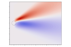
Figure 3. Significant wave height anomaly  $h_{s}(x,y)$ from (a,c,e,g) WW3 and (b,d, f,h) MA, for swell impinging on a Gaussian vortex. Each row corresponds to the indicated values of the directional spreading parameter $s$ of the incident wave spectrum, and the maximum velocity $U_m$ (in ${\rm m}\ {\rm s}^{-1}$). The corresponding non-dimensional parameters are given in table 1. The dashed circles have radius $r_{{v}}$ around the vortex centre. The solid lines in (b,d, f,h) indicate the caustics computed from (D6). The colour bars differ between rows but are the same within each row. White corresponds to $h_{s}=0$ in all plots. The customizable notebook that generates (h) by default can be accessed at https://www.cambridge.org/S0022112023006869/JFM-Notebooks/files/Figure-3.ipynb.
Typically, observations of the directional spreading for swell are in the range  $10^\circ \unicode{x2013}20^\circ$ (Ewans Reference Ewans2002), which corresponds to a range for $s$ between $16$ and $66$. In our experiments, setting $s=10$ and $s=40$ leads to directional spreading of $24^\circ$ and $12^\circ$, respectively, which correspond to very broad and very narrow swells.
Figures 3 and 4 show the significant wave height anomaly
 \begin{equation} h_{s}({\boldsymbol{x}})\stackrel{\text{def}}{=} H_{s}({\boldsymbol{x}})-H_{{s}\star} \end{equation}
for each combination of  $s$ and $U_m$. Because of our choice $H_{{s}\star } = 1$ m, $h_{s}$ in cm can be interpreted as the fractional change in significant wave height expressed as a percentage. A control run of WW3 in the absence of currents shows that $h_{s}$ is not exactly zero but decreases slowly with $x$. This is caused by the finite $y$-extent of the computational domain that leads to a wave forcing with compact support. To mitigate this numerical artefact, we compute the WW3 significant wave height anomaly as $h_{s}({\boldsymbol {x}}) = H_{s}({\boldsymbol {x}})-H_{s}^{ctrl}({\boldsymbol {x}})$, where $H_{s}^{ctrl}({\boldsymbol {x}})$ is the significant wave height of the current-free control run. See Appendix B for details.

Figure 4. Significant wave height anomaly  $h_s$ as a function of $y$ for (a,d) $x=r_v$, (b,e) $x=5r_v$, (c, f) $x=15 r_v$, and from WW3 (solid lines) and MA (see (4.5), dashed lines) in the set-up of figure 3. Results are shown for two sets of parameters $s$ and $U_m$ as indicated in (a,d). The range of $h_s$ differs between plots.
Figures 3 and 4 show that  $h_{s}$ has a wedge-like pattern in the wake of the vortex resulting from wave focusing and defocusing, with $h_{s} > 0$ mainly for $y > 0$, and $h_{s} < 0$ for $y < 0$. The pattern is not antisymmetric about $y=0$, and positive anomalies are larger than negative anomalies. These characteristics, which indicate a nonlinear response, are increasingly marked as $s$ and $U_m$ increase. Specifically, the parameter
 \begin{equation} \gamma = \frac{\varepsilon}{\delta} = \frac{U_m}{c_{{\star}}} \sqrt{\frac{s}{2}} \end{equation}
controls the degree of nonlinearity and hence of asymmetry. We discuss the two limiting regimes  $\gamma \ll 1$ and $\gamma \gg 1$ in § 5.
There is good overall agreement between WW3 and MA, even though in the case  $s=10$, the parameter $\delta = 0.447$ is only marginally small. The pattern is more diffuse for WW3 than for MA, with a less sharply defined wedge and a non-zero $h_{s}$ over a larger proportion of the domain. We attribute the differences to the finiteness of $\delta$ (they are more marked for $s=10$, $\delta = 0.447$ than for $s=40$, $\delta =0.224$), and to the limited spectral resolution of WW3 (simulations with degraded angular resolution lead to an even more diffuse $h_{s}$). The most conspicuous differences between WW3 and MA appear in the scattering region, where the non-zero $h_{s}$ obtained with WW3 appears to contradict the MA prediction that $h_{s} = 0$. The non-zero $h_{s}$ results from $O(\varepsilon,\delta )$ terms neglected by MA. Relaxing some of the approximations leading to (3.24) gives a heuristic correction to MA that captures the bulk of the difference with WW3 in the scattering region. We explain this in Appendix C.
As further demonstration of the MA approach, we provide a Jupyter notebook accessible at https://www.cambridge.org/S0022112023006869/JFM-Notebooks/files/Figure-3.ipynb, where users can customize the form of the current and the incoming wave spectrum to experiment with the resulting  $\int \mathcal {A}(x,y,k,\theta ) \, \mathrm {d} k$ and $h_{s}$.
4.2. Vortex dipole
A striking feature of the far-field spectrum and hence of  $H_{s}$ is that, according to MA, they depend on the flow only through the deflection $\varDelta (y)$ in (3.17), proportional to the integral of the vorticity along the direction of dominant wave propagation (the $x$-direction in our set-up). This implies that if the integrated vorticity vanishes because of cancellations between positive and negative contributions, the differences between far-field and incident fields are asymptotically small. This can be interpreted as a form of ‘vortex cloaking’, whereby an observer positioned well downstream of a flow feature is unable to detect its presence through changes in wave statistics. We demonstrate this phenomenon by examining the scattering of swell by vortex dipoles.
We consider two cases, corresponding to dipoles whose axes (the vectors joining the centres of positive and negative vorticity) are, respectively, perpendicular and parallel to the direction of wave propagation. The corresponding vorticity fields are chosen, up to a constant multiple, as the derivative of the Gaussian profile (4.1) with respect to  $y$ or $x$. Figure 5 shows the significant wave height anomaly obtained for the incident spectrum of § 4.1 with $s=40$ and dipoles with maximum velocity $U_m=0.8 {\rm m} \ {\rm s}^{-1}$.

Figure 5. Swell impinging on vortex dipoles with axes (a–c) perpendicular and (d–f) parallel to the dominant direction of wave propagation ( $x$-axis). The vorticity (colour) and velocity (vectors) are shown in (a,d), together with the significant wave height anomaly $h_{s}$ from WW3 in (b,e) and MA in (c, f). The directional spreading parameter is $s = 40$, and the maximum flow velocity is $0.8\ {\rm m}\ {\rm s}^{-1}$.
When the dipole axis is in the  $y$-direction (figures 5a–c), the deflection $\varDelta (y)$ does not vanish identically. As a result, $H_{s}$ is affected strongly by the flow, for our choice of parameters. This applies to both the MA and WW3 predictions, which match closely in the far field. When the dipole axis is in the $x$-direction (figures 5d–f), $\varDelta (y) = 0$. The MA prediction is then that $H_{s} = H_{{s}\star }$, i.e. $h_{s} = 0$ everywhere. The WW3 simulation is consistent with this, with only a weak signal in $h_{s}$.
In general, for a dipole with axis making an angle  $\alpha$ with the direction of wave propagation, the deflection $\varDelta (y)$ is proportional to $\sin \alpha$, and the cloaking effect is partial unless $\alpha = 0$.
5. Limiting cases
In this section, we return to the far-field asymptotics (3.22) for  $\mathcal {A}$ in terms of the scaled dependent variables in order to examine two limiting regimes characterised by extreme values of $\gamma = \varepsilon / \delta$. The regime $\gamma \ll 1$ corresponds to a weak flow and/or relatively broad spectrum, leading to a linear dependence of $h_{s}$ on the currents. The opposite regime $\gamma \gg 1$ corresponds to strong flow and/or a highly directional spectrum. The wave response is then highly nonlinear in the currents and, as we show below, controlled by the caustics that exist for pure plane incident waves ( $\gamma = \infty$). The ‘freak index’ of Heller et al. (Reference Heller, Kaplan and Dahlen2008), given by $\varepsilon ^{2/3}/\delta$, is the analogue of $\gamma$ for spatially extended, random currents.
5.1. Linear regime: $\gamma \ll 1$

For  $\gamma \ll 1$, we can expand (3.22) in Taylor series to obtain
 \begin{equation} \mathcal{A}(X,y,K,\varTheta) = \mathcal{A}_{{\star}}(K, \varTheta) - \gamma\,\varDelta(y - X \varTheta)\, \partial_\varTheta \mathcal{A}_{{\star}}(K, \varTheta) + O(\gamma^2). \end{equation}
This indicates that the flow induces the small correction  $- \gamma \,\varDelta (y - X \varTheta )\, \partial _\varTheta \mathcal {A}_{\star }(K, \varTheta )$ to the action of the incident wave. We deduce an approximation for $H_{s}$ by integrating (5.1) with respect to $K$ and $\varTheta$ to obtain $H_{s}^2$ followed by a Taylor expansion of a square root. Alternatively, we can carry out a Taylor expansion of the far-field approximation (3.29) of $H_{s}$, treating $\varDelta (y)$ as small. The result is best expressed in terms of the anomaly $h_{s}$, found to be
 \begin{equation} h_{s}(x,y) ={-} \frac{H_{s\star}}{2} \int D_s'(\theta) \, \varDelta(y-x \theta) \, \mathrm{d} \theta \end{equation}
after reverting to the unscaled variables and setting  $\gamma = 1$. This simple expression is evaluated readily once the flow, hence $\varDelta (y)$, and directional spectrum $D_{\star }(\theta )$ are specified. For the Gaussian vortex of § 4.1 and the directional spectrum in (2.6), the integration can be carried out explicitly, yielding
 \begin{equation} h_{s}(x,y)= \frac{H_{{s}\star} \kappa}{c_{{\star}} \sqrt{\rm \pi}}\,\frac{x^+ y \exp\!\left({-y^2/(2r_v^2+4x^2/s)}\right)}{(2 r_v^2+4x^2/s)^{3/2}}. \end{equation}
This formula makes it plain that  $h_{s}$ depends on space through $(x/\sqrt {s}, y)$, is antisymmetric about the $x$-axis, and is maximised along the curves $y=\pm \sqrt {r_v^2+2x^2/s}$. Decay as $|{\boldsymbol {x}}| \to \infty$ is slowest along these curves and proportional to $x^{-1}$.
We illustrate (5.3) and assess its range of validity by comparing it with MA for two sets of parameters in figure 6. The match is very good for  $s=10$ and $U_m = 0.4\ {\rm m}\ {\rm s}^{-1}$ (figures 6a,b), corresponding to $\gamma = 0.112$. It is less good for $s=40$ and $U_m = 0.8\ {\rm m}\ {\rm s}^{-1}$ (figures 6c,d), unsurprisingly since $\gamma = 0.447$ is not particularly small and the MA prediction is obviously far from linear, with a pronounced asymmetry. The curves $y=\pm \sqrt {r_v^2+2x^2/s}$ shown in the figure are useful indicators of the structure of $h_{s}$ for small enough $\gamma$.

Figure 6. Significant wave height anomaly  $h_{s}(x,y)$ for swell impinging on a Gaussian vortex: comparison between the predictions of (a,c) MA and (b,d) its $\gamma \to 0$ limit (see (5.3)). The set-up is as in figure 3, with parameters $s$ and $U_m$ (in ${\rm m}\ {\rm s}^{-1}$) as indicated. Dashed lines indicates the curves $y=\pm \sqrt {r_v^2+2x^2/s}$ where $h_{s}$ reaches maximum amplitudes according to (5.3).
5.2. Caustic regime: $\gamma \gg 1$

The limit  $\gamma \to \infty$ corresponds to an incident wave field that is almost a plane wave. It is natural to rescale variables according to $\varTheta \mapsto \gamma \varTheta$ and $X \mapsto \gamma ^{-1} X$ so that (3.22) becomes
 \begin{equation} \mathcal{A}(X,y,K,\varTheta) = \mathcal{A}_{{\star}}\left(K, \gamma\, \mathcal{S}(X,y,\varTheta) \right), \end{equation}
where
 \begin{equation} \mathcal{S}(X,y,\varTheta) \stackrel{\text{def}}{=} \varTheta - \varDelta(y - X \varTheta). \end{equation}
In  $(X,y,\varTheta )$-space, the $K$-integrated action is concentrated in a thin $O(\gamma ^{-1})$ layer around the surface $\mathcal {S}(X,y,\varTheta )=0$. Quantities such as $H_{s}$ obtained by integrating the action with respect to $\varTheta$ can be obtained by approximating the dependence of the right-hand side of (5.4) on $\mathcal {S}$ by $\delta ( \mathcal {S})$. This fails, however, when $(X,y,\varTheta )$ satisfy both
 \begin{equation} \mathcal{S}(X,y,\varTheta) = 0 \quad \text{and} \quad \partial_\varTheta \mathcal{S}(X,y,\varTheta)= 1 + X\,\varDelta'( y - X \varTheta) = 0. \end{equation}
The corresponding curves in the  $(X,y)$-plane are caustics near which $\int \mathcal {A}(X,y,K,\varTheta) \mathrm {d} K \,\mathrm {d} \varTheta$ is an order $\gamma ^{1/2}$ larger than elsewhere; correspondingly, $H_{s} = O(\gamma ^{1/4})$. In figure 7, the two caustics meet at a cusp point from opposite sides of a common tangent. The cusp point is located by the condition $\partial ^2_{\varTheta } \mathcal {S} = 0$, and the integrated action at the cusp point is $O(\gamma ^{2/3})$ so that $H_{s} = O(\gamma ^{1/3})$. We have verified numerically these $\gamma$ scalings at the caustics and at the cusp point by varying $s$ in the MA solutions.

Figure 7. Caustics for swell impinging on a Gaussian vortex: the caustics (D6) (solid lines) are superimposed onto the MA prediction of  $h_{s}$ for $U_m=0.8\ {\rm m}\ {\rm s}^{-1}$ and the indicated values of $s$. The dashed vertical lines correspond to the values $x = r_v$, $3r_v$ and $5 r_v$ used in figure 8.

Figure 8. Wavenumber-integrated action density  $\int \mathcal {A}(x,y,k,\theta ) \,\mathrm {d} k$ as a function of $y$ and $\theta$ for $x=r_v, 3r_v, 5r_v$ corresponding to the significant wave height shown in figure 7 for (a,c,e) $s=200$ and (b,d, f) $s=4000$. Line P1 in (d) corresponds to the values of $(x,y)$ of the cusp from where the caustics emanate; P2 and P3 are associated with points on each of the two caustics.
For the Gaussian vortex (4.1), the system (5.6a,b) can be solved to obtain an explicit equation for the caustics. This equation is derived in Appendix D and given by (D6). It describes two curves  $y(x)$ emanating from the cusp point at $x = x_c$ given by (D5). The caustics (which depend on $U_m$ but not on $s$) are indicated in figures 3(b,d, f,h). For the parameters of the figure, the caustics do not map regions of particularly large $h_{s}$. This is unsurprising since $\gamma$ is at most $0.447$.
To assess how large  $\gamma$, or equivalently $s$, needs to be for caustics to be the dominant feature of $H_{s}$, in figure 7 we show $h_{s}$ computed from MA for $U_m = 0.8\ {\rm m}\ {\rm s}^{-1}$ and $s = 200$ ( $\gamma = 1$, figure 7a) and $s=4000$ ( $\gamma = 4.47$, figure 7b). It is only for $s=4000$ that the caustics are evidently controlling the significant wave height pattern. We emphasise that $s=200$ and a fortiori $s=4000$ are unrealistically large values: observational estimates for $s$ in the open ocean seldom exceed $s=80$. We conclude that caustics are unlikely to play a role in real ocean conditions.
With academic rather than practical interest in mind, then, we show in figure 8 the integrated action  $\int \mathcal {A} \, \mathrm {d} k$ as a function of $y$ for three different values of $x$ (identified by dashed vertical lines in figure 7). The figure illustrates how caustics emerge from a fold singularity in the surface $\mathcal {S}(x,y,\theta )=0$ along which action is concentrated in the $(x,y,\theta )$ phase space. For $x = r_v$, the surface is a graph over $(x,y)$, and there are no caustics; for $x = x_c \approx 3 r_v$, the surface has a single point of vertical tangency (P1 in figure 8f) corresponding to the birth of caustics at a cusp in the $(x,y)$-plane; for $x = 5 r_c$, there are two points of vertical tangency, P2 and P3 in figure 8(h), corresponding to the two caustic curves. The picture is increasingly blurred as $s$ decreases (compare figures 8(a,c,e) with figures 8(b,d, f) and with figure 2), explaining the diminishing importance of caustics for $H_{s}$.
6. Discussion and conclusion
The main results in this study are obtained by approximate solution of the wave-action equation in the four-dimensional position–wavenumber space. The organizing principle identified by the analysis is that scattering of SGWs by spatially compact currents results in the deflection function  $\varDelta (y)$ in (3.17). Although $\varDelta$ varies linearly with the vertical vorticity of the currents, it figures in a nonlinear transformation of the action density. This nonlinear transformation produces the modulation of the significant wave height $H_{s}$ behind the scattering region, e.g. the expression for $H_{s}$ in (3.29). Quantities that depend on other moments (e.g. Stokes drift) behave similarly and could be inferred readily from our explicit forms (3.15) and (3.22) for the wave-action density.
While we have obtained these results for deep-water SGWs, they apply essentially unchanged to other two-dimensional waves with isotropic dispersion relation such as finite-depth SGWs or Poincaré waves. The conclusions that we draw about  $H_{s}$ can also be rephrased in terms of other root-mean-square quantities relevant to waves other than SGWs. With a little effort, the approach that we adopt, based on the matched asymptotics treatment of the wave-action equation, could be extended further to three-dimensional waves and to anisotropic dispersion relations. Our results could be extended easily to account for vertically sheared currents using the modified dispersion relation of Kirby & Chen (Reference Kirby and Chen1989) (which involves a Doppler shift term that is nonlinear in ${\boldsymbol {k}}$).
In addition to the WKB approximation used to derive the action conservation equation (2.1), there are two independent approximations involved:
(a) the current speed is much less than the group velocity of the incident swell;
(b) swell with small directional spreading is incident on a region of spatially compact currents, e.g. an axisymmetric vortex or a vortex dipole.
Provided that (a) and (b) are satisfied, the approximate solution of the wave-action equation compares well with numerical solutions provided by WW3.
Approximation (a) is usually justified. To challenge (a), one must consider current speeds such as  $2\ {\rm m}\ {\rm s}^{-1}$, e.g. observed as a peak current speed in the Agulhas system (Quilfen & Chapron Reference Quilfen and Chapron2019). Swell with 100 m wavelength has group velocity ${\sim }6\ {\rm m}\ {\rm s}^{-1}$, so the small parameter in (a) is as large as $1/3$. In less extreme cases, approximation (a) will be satisfied.
Approximation (b) is less secure: ocean swell is not sufficiently unidirectional to strongly justify (b) – e.g. see the  $\delta$ column in table 1. Over long distances, the continuous scattering by uncorrelated currents leads to a broadening of the angular spectrum. When approximation (a) applies, this broadening is described by the directional diffusion equation for wave action derived by Villas Bôas & Young (Reference Villas Bôas and Young2020). This diffusion process is one of the mechanisms that makes swell with very small values of $\delta$ unlikely. However, our computations for a Gaussian vortex indicate that our asymptotic results are reliable for the moderately small values of $\delta$ typical of swell.
Because of the relatively large directional spreading of ocean swell, the mathematical ideal of a sharp wave caustic is not realised. Instead, the caustic singularity is ‘washed out’ (Heller et al. Reference Heller, Kaplan and Dahlen2008). Behind a vortex, we find instead an elongated streaky pattern in  $H_{s}$.
Our results show that  $H_{s}$ behind an axisymmetric vortex with parameters in table 1 has spatial variation as large as ${\pm }30\,\%$ of the incident constant value $H_{{s}\star }$. Spatial inhomogeneities in $H_{s}$ of this magnitude are important for wave breaking and exchange of momentum, heat and gas between the ocean and atmosphere. For example, airborne observations of the ocean surface by Romero et al. (Reference Romero, Lenain and Melville2017) indicate that ${\pm }30\,\%$ variations in $H_{s}$ are associated with an order of magnitude increase in whitecap coverage.
The directional diffusion equation of Villas Bôas & Young (Reference Villas Bôas and Young2020) uses only approximation (a). One does not need to assume that the wave field is strongly unidirectional or that the currents are spatially compact. Moreover, the directional diffusion equation is obtained without detailed consideration of the perturbations to the action spectrum that accompany wave scattering. But there is useful information hiding in these unexamined perturbations to the action spectrum. We are engaged currently in extracting these perturbations, calculating the attendant spatial variability to  $H_{s}$, and relating the statistics of these fluctuations in $H_{s}$ to those of the surface currents. These future developments promise to explain numerical experiments that identify relations between the spectral slopes of surface-current spectra and those of significant wave height (Villas Boâs et al. Reference Villas Boâs, Cornuelle, Mazloff, Gille and Ardhuin2020).
Supplementary material
Computational Notebook files are available as supplementary material at https://doi.org/10.1017/jfm.2023.686 and online at https://www.cambridge.org/S0022112023006869/JFM-Notebooks/files/Figure-3.ipynb.
Acknowledgements
We thank V. Shrira for conversations about this work.
Funding
J.V. and H.W. are supported by the UK Natural Environment Research Council (grant NE/W002876/1). A.B.V.B. is supported by NASA award 80NSSC23K0979 through the International Ocean Vector Winds Science Team. W.R.Y. is supported by the National Science Foundation award 2048583.
Declaration of interests
The authors report no conflict of interest.
Data availability statement
The WW3 configuration files applied in this work can be found at https://github.com/biavillasboas/SwellVortex.
Appendix A. Incident spectrum
We use the separable spectrum
 \begin{equation} \mathcal{F}_{\!\star}(k,\theta)= \zeta_{{rms}\star}^2\,F_\star(k)\, D_{{\star}}(\theta) . \end{equation}
The wavenumber function in (A1) is
 \begin{equation} F_\star(k)\stackrel{\text{def}}{=} \frac{2}{\mathrm{erfc}(-\sigma_{{\star}}/\sqrt{2}\,\delta_{\sigma})} \frac{\exp({ -(\sigma - \sigma_{{\star}})^2/2 \delta_{\sigma}^2})}{\sqrt{2 {\rm \pi}\delta_{\sigma}^2} } \, \frac{1}{k}\,\frac{\mathrm{d} \sigma}{\mathrm{d} k}, \end{equation}
where  $\mathrm {erfc}$ is the complementary error function. It corresponds to a Gaussian spectrum in frequency truncated at $\sigma =0$. The angular part of the spectrum in (A1) is
 \begin{equation} D_{{\star}}(\theta) \stackrel{\text{def}}{=} \frac{\varGamma(s+1)}{2\sqrt{\rm \pi}\,\varGamma(s+\tfrac{1}{2})} \cos^{2s} \left(\frac{\theta}{2}\right) \end{equation}
(Longuet-Higgins et al. Reference Longuet-Higgins, Cartwright and Smith1963), which corresponds to incoming waves spread around  $\theta =0$. The four parameters in this model spectrum are the root-mean-square sea-surface displacement $\zeta _{{rms}\star }$, the peak radian frequency $\sigma _{\star }=\sqrt {g k_{\star }}$, the spectral width $\delta _{\sigma }$, and the directional spreading parameter $s$. Normalisation is ensured with
 \begin{equation} \int_{-{\rm \pi}}^{\rm \pi} D_{{\star}}(\theta) \,\mathrm{d} \theta = 1 \quad \text{and} \quad \int_0^\infty F_\star(k)\,k \, \mathrm{d} k =1. \end{equation}
 In the narrow-band limit  $\delta _{\sigma }/\sigma _{\star } \ll 1$ and $s \gg 1$, the spectrum is approximated by (2.6) with $\delta _k = 2 \delta _\sigma \sqrt {k_{\star }/g}$ and $\delta _{\theta }=\sqrt {2/s}$. The parameter $\delta _{\theta }$ captures the standard deviation in the angular distribution, which is the definition of ‘directional spreading’ (Kuik, Van Vledder & Holthuijsen Reference Kuik, Van Vledder and Holthuijsen1988). We note that the expressions for directional spreading are sometimes formally different, but equivalent to our expression for $\delta _{\theta }$ at large $s$. For example, another popular way to state the definition for a generic directional distribution is
 \begin{equation}
\sigma_{\theta} \stackrel{\text{def}}{=} \big[2\big(1-(a^2+b^2)^{1/2}\big)\big]^{1/2},
\end{equation}
\begin{equation}
\sigma_{\theta} \stackrel{\text{def}}{=} \big[2\big(1-(a^2+b^2)^{1/2}\big)\big]^{1/2},
\end{equation}
where
 \begin{equation} a=\int\cos{\theta}\,D_{{\star}}(\theta)\, \mathrm{d} \theta \quad \textrm{and} \quad b=\int\sin{\theta}\,D_{{\star}}(\theta)\, \mathrm{d} \theta \end{equation}
(Villas Boâs et al. Reference Villas Boâs, Cornuelle, Mazloff, Gille and Ardhuin2020). Using the expression for  $D_{\star }$ in (2.6), we can compute the integrals in (A6a,b) analytically, getting $a=\mathrm {e}^{-1/s}$ and $b=0$. Therefore,
 \begin{equation} \sigma_{\theta}^2=2(1-\mathrm{e}^{{-}1/s}) \to 2/s \quad \textrm{as} \ s\to \infty. \end{equation}
Thus the definition of  $\sigma _{\theta }$ in (A5) indeed agrees with the parameter $\delta _{\theta }$ at large $s$.
$s$.
Appendix B. Set-up of WAVEWATCH III
We compare our results with numerical simulations from an idealised set-up of WW3 that integrates the action balance equation (2.1). Here, we focus on freely propagating swell-type waves, so the effects of wind forcing, nonlinear interactions and wave breaking are ignored (e.g. Villas Boâs et al. Reference Villas Boâs, Cornuelle, Mazloff, Gille and Ardhuin2020). We use WW3 version v6.07.1 (https://github.com/NOAA-EMC/WW3/releases/tag/6.07.1) to solve (2.1) on a  $1000\ {\rm km}\times 1000\ {\rm km}$ Cartesian domain with 5 km grid spacing. To resolve swells with $s=10$ and $40$, the spectral grid has 80 directions and 32 frequencies. Larger values of $s$ (i.e. narrower directional spreading) would require higher directional resolution for the model to converge. We use the global integration time step 200 s, spatial advection time step 50 s, spectral advection time step 12 s, and minimum source term time step 5 s. We verified that decreasing the time stepping or the spatial grid spacing does not significantly change the results (not shown).
All simulations are initialised with the narrow-banded wave spectrum in (A1). Waves enter the domain from the left boundary with initial mean direction  $\theta = 0^\circ$ (propagating from left to right), directional spreading parameter $s=10$ or $s=10$, peak frequency $\sigma _{\star } = 0.61 {\rm rad}\ {\rm s}^{-1}$ (peak period 10.3 s), spectral width $\delta _{\sigma } = 0.04$, and $H_{{s}\star } = 1$ m. The boundary condition at the left boundary is kept constant throughout the experiment, and each experiment is run until steady state is reached.
As mentioned in § 4.1, a control run is conducted in the absence of currents. Although there is no scattering from the currents, a non-uniform  $h_{s}^{ctrl}=H_{s}^{ctrl}-H_{{s}\star }$ arises, due to the limited domain size in $y$, which leads to a reduction of incident wave action from waves arriving from large $|y|$ – an effect that is more pronounced at large $x$. As $s$ increases, the action density in the incident spectrum is more concentrated in the x-direction, leading to less leakage of wave action through the top and bottom boundaries, and a more spatially uniform $h_{s}^{ctrl}$. This leakage of wave action corresponds to a reduction of 5 % in $h_{s}^{ctrl}$ for $s=10$, and 2 % for $s=40$ towards the right-hand side boundary.
Appendix C. MA–WW3 mismatch in the scattering region
We develop a heuristic correction to MA that we show captures the non-zero  $h_{s}$ in the scattering region. First, we note that the non-zero $h_{s}$ in the scattering region from WW3 appears localised, likely caused by the term proportional to $\partial _k\mathcal {A}$ in (3.9), as the terms proportional to $\partial _{\theta }\mathcal {A}$ result in non-local effects. This observation is confirmed by a WW3 run, which we refer to as WW3 $^{-}$, where the term in $\partial _k \mathcal {A}$ is suppressed in the wave-action equation, yielding a more uniform $h_{s}$ in the scattering region (see figure 9d). We then recall that in the MA solution, the insignificance of the $\partial _k\mathcal {A}$ term is due to the approximation of a single dominant wavenumber in the steps leading to (3.24). We thus return to the approximation (3.12) of the wave-action transport equation in the scattering region and relax the approximation of replacing $k$ by $k_{\star }$. We focus on the $\theta$-integrated action
 \begin{equation} \mathcal{B}({\boldsymbol{x}},k) = \int \mathcal{A}({\boldsymbol{x}}, {\boldsymbol{k}}) \, \mathrm{d} \theta, \end{equation}
which satisfies
 \begin{equation} c(k) \, \partial_x \mathcal{B} - U_x({\boldsymbol{x}})\,k \,\partial_k \mathcal{B} = 0. \end{equation}
Noting that  $c(k) = g^{1/2} k^{-1/2}/2$, we solve this equation using the method of characteristics to find
 \begin{equation} \mathcal{B}({\boldsymbol{x}},k) = \mathcal{B}_\star\big(\big(k^{{-}1/2} - g^{{-}1/2}\,U({\boldsymbol{x}}) \big)^{{-}2} \big). \end{equation}
The significant wave height is deduced by integration as
 \begin{equation} H_{s}({\boldsymbol{x}})
= \left(\frac{16}{g^{1/2}} \int \mathcal{B}_\star\big(
\big(k^{{-}1/2} - g^{{-}1/2}\,U({\boldsymbol{x}}) \big)^{{-}2}
\big) k^{3/2} \, \mathrm{d} k \right)^{1/2}.
\end{equation}
\begin{equation} H_{s}({\boldsymbol{x}})
= \left(\frac{16}{g^{1/2}} \int \mathcal{B}_\star\big(
\big(k^{{-}1/2} - g^{{-}1/2}\,U({\boldsymbol{x}}) \big)^{{-}2}
\big) k^{3/2} \, \mathrm{d} k \right)^{1/2}.
\end{equation}
We now change the integration variable, taking advantage of the localisation of  $\mathcal {B}_\star (k)$ to ignore the corresponding change in the lower limit of integration, and obtain
 \begin{align}
H_{s}({\boldsymbol{x}}) &=
\left( \frac{16}{g^{1/2}} \int \mathcal{B}_\star(k) (k^{{-}1/2} + g^{{-}1/2}\,U({\boldsymbol{x}}))^{{-}6} k^{{-}3/2} \, \mathrm{d} k \right)^{1/2}
\nonumber\\ &= \left( \frac{16}{g^{1/2}} \int \mathcal{B}_\star(k)\,k^{3/2} (1 + k^{1/2}
g^{{-}1/2}\,U({\boldsymbol{x}}))^{{-}6} \,
\mathrm{d} k \right)^{1/2} \nonumber\\ &= \Bigg(
\frac{16}{g^{1/2}} \int \mathcal{B}_\star(k)\,k^{3/2}
\Bigg(1 +
\frac{U({\boldsymbol{x}})}{2\,c(k)}\Bigg)^{{-}6}
\, \mathrm{d} k \Bigg)^{1/2}.
\end{align}
\begin{align}
H_{s}({\boldsymbol{x}}) &=
\left( \frac{16}{g^{1/2}} \int \mathcal{B}_\star(k) (k^{{-}1/2} + g^{{-}1/2}\,U({\boldsymbol{x}}))^{{-}6} k^{{-}3/2} \, \mathrm{d} k \right)^{1/2}
\nonumber\\ &= \left( \frac{16}{g^{1/2}} \int \mathcal{B}_\star(k)\,k^{3/2} (1 + k^{1/2}
g^{{-}1/2}\,U({\boldsymbol{x}}))^{{-}6} \,
\mathrm{d} k \right)^{1/2} \nonumber\\ &= \Bigg(
\frac{16}{g^{1/2}} \int \mathcal{B}_\star(k)\,k^{3/2}
\Bigg(1 +
\frac{U({\boldsymbol{x}})}{2\,c(k)}\Bigg)^{{-}6}
\, \mathrm{d} k \Bigg)^{1/2}.
\end{align}
At this point, we can approximate  $c(k)$ by $c_\star$ in the small $O(\varepsilon )$ term $U({\boldsymbol {x}})/(2\,c(k))$ and use two binomial expansions to obtain
 \begin{equation} H_{s}({\boldsymbol{x}}) \approx H_{{s}\star} \left(1 - \frac{3U({\boldsymbol{x}})}{2 c_{{\star}}} \right). \end{equation}
We emphasise the heuristic nature of this approximation (MA $^+$), which is formally no more accurate than the MA approximation $H_{s}({\boldsymbol {x}})=H_{{s}\star }$ since it neglects some, though not all, $O(\delta )$ terms. Nonetheless, it captures most of the significant wave height anomaly close to the Gaussian vortex, as figure 9 demonstrates under parameters $s=40$ and ${U_m=0.8\ {\rm m} {\rm s}^{-1}}$.

Figure 9. Significant wave height anomaly hs computed from (a) WW3, (b) MA (same as figures 3g,h), (d) WW3 $^-$ (where the term proportional to $\partial _k \mathcal {A}$ is switched off) and (e) MA $^+$ as in (C6). Panels (c) and (f) show the differences between (a) and (b), and (a) and (e), respectively. All plots have the same colour bar.
Appendix D. Caustics for the Gaussian vortex
In the Gaussian vortex example, we can derive the locations of the caustics in the  $(x,y)$-plane analytically. Using expression (4.3) for $\varDelta (y)$, and introducing the functions
 \begin{equation} w(x,y) \stackrel{\text{def}}{=} -(y-x\theta)^2/r_v^2 \end{equation}
and
 \begin{equation} q(x) \stackrel{\text{def}}{=}-2{\rm \pi} r_v^4 c_{{\star}}^2/(x^2 \kappa^2), \end{equation}
we can write (5.6a,b) defining the caustics as
 \begin{equation} \theta-\frac{\kappa}{\sqrt{2{\rm \pi}}\,r_vc_{{\star}}}\,\mathrm{e}^{w/2}=0 \end{equation}
and
 \begin{equation} w\,\mathrm{e}^{w}=q. \end{equation}
Equation (D4) relates  $w$ to $q$, and takes the standard form defining the Lambert $W$-functions (see Olver Reference Olver, Lozier, Boisvert and Clark2010, (4.13.1)). This equation has two branches of solutions $w=W_{i}(q)$, $i=0, -1$, when $0 < -q < \mathrm {e}$, and no solutions when $-q > \mathrm {e}$ ( $q < 0$ by definition (D2)). The two branches meet at $q=-\mathrm {e}^{-1}$, which corresponds to
 \begin{equation} x=x_c\stackrel{\text{def}}{=} \sqrt{2{\rm \pi}\mathrm{e}}\,r_v^2c_{{\star}}/\kappa. \end{equation}
Physically, the two branches  $w=W_{i}(q)$ correspond to two caustic lines in the $(x,y)$-plane that emanate from a cusp point with $x=x_c$. The equation of the caustics is found using (D1) and (D3) as
 \begin{equation} y=\frac{\kappa x \exp({W_{i}(q(x))/2})}{\sqrt{2{\rm \pi}}\,r_vc_{{\star}}}+\sqrt{-W_{i}(q(x))}\,r_v,\quad x\geqslant x_c. \end{equation}
The cusp point is at  $(x,y)=(x_c,2 r_v)$.
The asymptotic form of the caustics for  $x \to \infty$ is obtained readily by noting that $q(x) \to 0^-$ as $x \to \infty$, and then that $W_0(q) \to 0$ and $W_{-1}(q) \sim \ln (-q)$. Thus the $i=0$ caustic asymptotes to a straight line, and the $i=-1$ caustic to $y \sim (2 \ln x)^{1/2}$.


 Open access