


1. Introduction
Microfluidic lab-on-a-chip devices allow users to sample and sort cells, engineer flow patterns or fabricate metamaterials (Schaaf, Rühle & Stark Reference Schaaf, Rühle and Stark2019). One phenomenon that has attracted considerable attention over the past decades is the utilisation of fluid–fluid interfaces in many engineering and microfluidics applications, including encapsulation, coating and dissolution processes (Magnaudet & Mercier Reference Magnaudet and Mercier2020), micro-reactions (Rivero-Rodriguez & Scheid Reference Rivero-Rodriguez and Scheid2018), flow batteries (Ruiz-Martín et al. Reference Ruiz-Martín, Moreno-Boza, Marcilla, Vera and Sánchez-Sanz2022), fabrication of complex materials (Isa, Samudrala & Dufresne Reference Isa, Samudrala and Dufresne2014) or biotechnology and biomedicine (Hütten et al. Reference Hütten, Sudfeld, Ennen, Reiss, Hachmann, Heinzmann, Wojczykowski, Jutzi, Saikaly and Thomas2004). In addition, the development of complex fabrication techniques often implies the utilisation of particles embedded in one or both of the fluids that eventually cross the liquid–liquid interface, with encapsulation and coating being some of the most relevant applications (Kawano et al. Reference Kawano, Hashimoto, Ihara and Shin1996; Pitois, Moucheront & Weill Reference Pitois, Moucheront and Weill1999; Tsai et al. Reference Tsai, Wexler, Wan and Stone2011; Sinha et al. Reference Sinha, Mollah, Hardt and Ganguly2013; Hadikhani et al. Reference Hadikhani, Hashemi, Balestra, Zhu, Modestino, Gallaire and Psaltis2018). In these situations, the couple effects between the hydrodynamic drag, inertial effects, interface deformation and shear or strain near the walls of the channels drive the movement of a particle in a non-quiescent flow towards or away of the fluid–fluid interface at low Reynolds numbers (Magnaudet & Mercier Reference Magnaudet and Mercier2020).
The control of the dynamics of these particles near fluid interfaces or elastic membranes enables, for instance, the preparation of high-quality crystals, plays an important role on the fabrication of foams and emulsions (Bresme & Oettel Reference Bresme and Oettel2007) and enables the study of swimmers and particles near elastic interfaces (Rallabandi et al. Reference Rallabandi, Oppenheimer, Ben Zion and Stone2018). In the latter case, the compliance of the membrane couples the hydrodynamic field with the hydroelastic forces of the membrane, breaking symmetry and inducing repulsive forces that separate the particle from the membrane with a velocity that changes with the resistance to bending and shearing of the membrane (Daddi-Moussa-Ider, Lisicki & Gekle Reference Daddi-Moussa-Ider, Lisicki and Gekle2017; Rallabandi et al. Reference Rallabandi, Oppenheimer, Ben Zion and Stone2018).
The problem of particles moving near fluid–fluid interfaces has been analysed extensively in the limit in which inertial forces are considerably larger than capillary and viscous forces. The paper by Magnaudet & Mercier (Reference Magnaudet and Mercier2020) offers an excellent review of the recent work on the matter when the body (bubble, droplet or rigid body) impinges perpendicularly into a free surface. A closely related problem with more relevance in other applications, such as liquid filters (Sinha et al. Reference Sinha, Mollah, Hardt and Ganguly2013) or conformal coating (Moon et al. Reference Moon, Hakimi, Hwang and Tsai2014), is that of particles moving parallel to a fluid–fluid interface inside a channel that, eventually, may cross the interface to emerge on the other phase. Available experiments and simulations have focused on bodies moving in a quiescent fluid, but very little is known about the interaction between the tangential displacement of the particle and fluid–fluid interfaces or elastic membranes. Experiments with particles travelling along an air–water interface indicated that the drag coefficient depends on the deformation of the interface (Petkov et al. Reference Petkov, Denkov, Danov, Velev, Aust and Durst1995). Numerically, the work by Loudet et al. (Reference Loudet, Qiu, Hemauer and Feng2020) simulated a particle embedded in a fluid–fluid interface deformed by the weight of the particle. Their numerical results, using a non-realistic uniform velocity profile at both the inlet and outlet sections of the computational domain, showed that large drag forces are not correlated with large interfacial distortions.
The presence of the interface affects the velocity and pressure fields even in the limit of zero Reynolds number. When two unbounded immiscible fluids are considered (Lee, Chadwick & Leal Reference Lee, Chadwick and Leal1979; Bławzdziewicz, Ekiel-Jeżewska & Wajnryb Reference Bławzdziewicz, Ekiel-Jeżewska and Wajnryb2010), the problem can be tackled using asymptotic methods in the limit of very large surface tension, to show that the drag force on the particle is larger than in the case of an single infinite fluid.
Taking advantage of the linearity of the equations in the limit of zero Reynolds number, Berdan & Leal (Reference Berdan and Leal1982) obtained the shape of the interface considering the effect of gravity in the limit of small capillary number  $Ca=\mu _2 \bar {u}/\gamma$, with $\mu _2$ the viscosity of the fluid in which the sphere is embedded, $\bar {u}$ the characteristic velocity and $\gamma$ the surface tension of the fluid–fluid interface. In their semi-analytical calculations they obtained a non-symmetric interface deformation in which the surface tension allowed very broad deformation with small curvature. This deformation induced a transverse force that promotes the migration of the sphere. This migration is similar to that induced by inertial effects when the Reynolds of the problem is small but non-zero (Segré & Silberberg Reference Segré and Silberberg1962a,Reference Segré and Silberbergb). A detailed literature review of the dynamics of particles, drops and bubbles can be found in Rivero-Rodriguez & Scheid (Reference Rivero-Rodriguez and Scheid2018), with some examples of utilisation of these effects for fascinating applications in medicine, chemistry and engineering given by Zhang et al. (Reference Zhang, Yan, Yuan, Alici, Nguyen, Warkiani and Li2016) and Di Carlo (Reference Di Carlo2009).
Motivated by these applications, in this paper we aim to compute the vertical force exerted on a rigid particle moving with terminal velocity  $V$ and angular velocity $\varOmega$ inside a two-dimensional channel parallel to a fluid–fluid interface. The present work is organised as follows. First, the problem under study is formulated in § 2 including the equations governing the fluid flow and the appropriate boundary conditions. The range of parameters selected in the computations presented throughout the paper is discussed in this section in terms of the stability of the interface. Section 3 considers the problem in the pure inertial regime in which the interface is considered non-deformable. Section 4 tackles the pure capillary regime $Re=0$ considering a deformable interface and studies asymptotically the limits of very large and very small surface tension.
2. Formulation of the problem
The formulation here presented examines the effect of shear and surface tension on the dynamics of moving particles in the presence of deformable fluid interfaces. We considered two immiscible liquids flowing in a channel with height  $h$. The two liquids form an interface that is located at $y=\varGamma$, with subscripts $1$ and $2$ referring to the lower and upper fluid, respectively. The total volumetric flow rate of the two liquids is $Q=Q_1+Q_2$ and we assume that both liquids have equal density $\rho =\rho _1=\rho _2$ but different viscosity $\mu _1 \ne \mu _2$.
The experiments by Lee et al. (Reference Lee, Amini, Stone and Di Carlo2010) motivate the configuration of the problem sketched in figure 1. In our computations, a train of particles of diameter  $d$ travels at its terminal velocity $V$ in the upper fluid forming a periodic flow structure with a single line of particles, with each particle separated by a distance $L$ from the closest neighbour. The distance $L$ is constant and will be changed in our simulations to consider the effect reported by Lee et al. (Reference Lee, Amini, Stone and Di Carlo2010) when the height of the channel was changed. The transverse location of the particle depends on the intensity of a uniform volumetric force $\boldsymbol {f}$ acting on both liquids.

Figure 1. Schematics of the flow configuration, including the geometrical and fluid-dynamical relevant parameters.
To describe the motion of the particle, we use a reference system attached to a particle that moves at its terminal velocity  $V$ so that the centre of the particle is located at $x=x_p=0$ and $y=y_p$. To write the problem in non-dimensional form, we choose the channel height $h$, the average velocity $\bar {u}=Q/h$ and $p_c=\mu _2 \bar {u}/h$ as the characteristics length, velocity and pressure to define the non-dimensional variables. The average velocity $\bar {u}$ and the properties of fluid 2 define the Reynolds number of the flow $Re=\rho Q/\mu _2$ and the capillary number $Ca=\mu _2 Q/\gamma$. Hereafter, all new variables refer to non-dimensional variables and the previously introduced refer to their non-dimensional counterparts scaled with their characteristic values defined previously. Introducing the non-dimensional variables, we obtain the non-dimensional continuity and momentum equations, yielding
 $$\begin{gather} \boldsymbol{\nabla}\boldsymbol{\cdot}\boldsymbol{v}_i = 0, \end{gather}$$
 $$\begin{gather}Re \, \boldsymbol{v}_i\boldsymbol{\cdot}\boldsymbol{\nabla} \boldsymbol{v}_i = \boldsymbol{\nabla}\boldsymbol{\cdot}\hat{\boldsymbol{T}}_i , \end{gather}$$
where  $\hat {\boldsymbol {T}}_i = - \hat {p}_i \boldsymbol{\mathsf{I}}+ \mu (\boldsymbol {\nabla } \boldsymbol {v}_i +\boldsymbol {\nabla }\boldsymbol {v}_i^{\rm T})$ and with $\hat {p}_i = p_i - \boldsymbol {f}\boldsymbol {\cdot }(\boldsymbol {x}-\boldsymbol {x}_{p})$ being the reduced pressure. The uniform volumetric force $\boldsymbol {f}$ is assumed to have only non-zero vertical component $\boldsymbol {f}= f \boldsymbol {e}_y$. The interface separating both fluids is described by the function $\varGamma =\varGamma (x)$ and defines each fluid domain $\boldsymbol {x} \in \mathcal {V}$, as indicated in figure 1. Consequently with this definition, the viscosity ratio in (2.2) is $\mu =\mu _1/\mu _2$ if $y < \varGamma$ and $\mu =1$ if $y > \varGamma$.
To identify the position of both the particle and the interface, we define the normalised variable  $\xi = [ y_p-(\varGamma _{L/2}+d/2) ] / [ 1-(d+\varGamma _{L/2}) ]$ and $\eta =\varGamma _{L/2}/(1-d)$, with $\varGamma _{L/2}=\varGamma (L/2)$. The variable $\xi$ ranges between $0 \leqslant \xi \leqslant 1$ and the two extreme values of $\xi$ corresponds to the particle touching the interface $y_p=\varGamma _{L/2}+d/2$ when $\xi =0$ or the channel wall $y_p=1-d/2$ when $\xi =1$, respectively (see figure 2). The normalised position of the interface $0\leqslant \eta \leqslant 1$ defines the extreme cases in which only fluid 2 runs through the channel $\eta =0$ and the case in which the particle is squeezed between the interface and the upper wall $\eta =1$, as illustrated in figure 2.

Figure 2. Definition of the normalised position of the (a,b) particle  $\xi$ with arbitrary $\eta$ and (c,d) of the interface $\eta$.
2.1. Boundary conditions
The system of equations given above in (2.1) and (2.2) is complemented with appropriate boundary conditions. In the reference frame attached to the particle, the velocity of the liquids at the walls  $y=0$ and $y=1$ is written as $\boldsymbol {v}_i=-V \boldsymbol {e}_{\boldsymbol {x}}$. Considering that the particle centre is located at $x=x_p=0$, we impose periodicity conditions so that
 \begin{equation} \left.\boldsymbol{v}\right|_{L/2} = \left.\boldsymbol{v}\right|_{{-}L/2}, \quad \left.\partial_x \boldsymbol{v}\right|_{L/2} = \left.\partial_x \boldsymbol{v}\right|_{{-}L/2}, \quad \left.\hat{p}\right|_{L/2}= \left.\hat{p}\right|_{{-}L/2} - \Delta p. \end{equation}
The pressure drop  $\Delta p$ and interface position are obtained by imposing the flow rates as total flow rate and flow ratios
 $$\begin{gather} \int_{0}^{\varGamma} (u_1+V) \,\mathrm{d} y + \int_{\varGamma}^{1} (u_2+V) \,\mathrm{d} y = 1 , \end{gather}$$
 $$\begin{gather}\int_{0}^{\varGamma} (u_1+V) \,\mathrm{d} y = \frac{Q_1}{Q_2} \int_{\varGamma}^{1} (u_2+V) \,\mathrm{d} y , \end{gather}$$
at any arbitrary section, for example  $x=L/2$. The terminal velocity $V$ is determined by imposing zero force on the particle in $x$ direction
 \begin{equation} \int_{\varSigma_p} \boldsymbol{e}_{\boldsymbol{x}}\boldsymbol{\cdot}\hat{\boldsymbol{T}}_2\boldsymbol{\cdot}\boldsymbol{n}_p =0 \end{equation}
with  $\boldsymbol {n}_p$ a unit-length vector normal to the surface of the particle $\varSigma _p$ pointing towards the fluid. The non-slip and zero net torque conditions are applied to determine the motion of the rigid particles,
 $$\begin{gather} \boldsymbol{v}_{2}(\boldsymbol{x}) = \boldsymbol{\varOmega} \times (\boldsymbol{x}-\boldsymbol{x_p}) \quad \text{at} \ \varSigma_{p} \end{gather}$$
 $$\begin{gather}\boldsymbol{0} = \int_{\varSigma_{p}} \boldsymbol{n}_p\boldsymbol{\cdot}\left\{ \hat{\boldsymbol{T}}_2 \times (\boldsymbol{x}-\boldsymbol{x_p})\right\}\boldsymbol{\cdot}\boldsymbol{e}_z \,{\rm d}\varSigma, \end{gather}$$
with  $\boldsymbol {\varOmega }= \varOmega \boldsymbol {e}_z$ and $\boldsymbol {e}_z=\boldsymbol {e}_x \times \boldsymbol {e}_y$. The implicit equation $q(x,y,t) =\varGamma (x,t)-y=0$ describes the location of the interface. Because $q=0$ on the interface at all times, the material derivative must satisfy
 \begin{equation} \boldsymbol{v}_2\boldsymbol{\cdot}\boldsymbol{n} = 0 \quad \text{at} \ \varGamma, \end{equation}
with  $\boldsymbol {n}=\boldsymbol {\nabla } q/|\boldsymbol {\nabla } q|=(\varGamma _x,-1)/(1+\varGamma _x^2)^{1/2}$ the unit-length vector normal to the surface $\varGamma$ pointing from fluid 2 towards fluid 1. At the fluid–fluid interface we impose the continuity of velocities and the jump condition on the stress tensor,
 \begin{equation} [\boldsymbol{v}] =\boldsymbol{0}, \quad \boldsymbol{n}\boldsymbol{\cdot}[ \hat{\boldsymbol{T}}] = Ca^{{-}1} (-\boldsymbol{n} \boldsymbol{\nabla}\boldsymbol{\cdot}\boldsymbol{n}) , \end{equation}
with  $Ca=\mu _2 \bar {u}/\gamma$ the capillary number, $\gamma$ the surface tension and the brackets indicating the jump of the variable included between them $[{\mathcal {L}}]={\mathcal {L}}_2-{\mathcal {L}}_1$. To compute the force per unit volume $f$ necessary to keep the particle at a given vertical position $\xi$, we impose equilibrium of vertical forces on the particle, yielding
 \begin{equation} \int_{\varSigma_p} \boldsymbol{e}_y\boldsymbol{\cdot}\hat{\boldsymbol{T}}_2\boldsymbol{\cdot}\boldsymbol{n}_p \,\mathrm{d} \varSigma - f \mathcal{V}_p = 0 , \end{equation}
where  $\mathcal {V}_p$ is the volume of the particle. In previous expression, the first term stands for the hydrodynamic force exerted by the fluid on the particle. The second is the external body force and represents, for example, buoyancy in the presence of a gravity field.
Once the problem is formulated in non-dimensional form, and taking into account that the density ratio is considered unity  $\rho _{2}/\rho _{1}=1$ and the size of the particle is set constant and equal to $d=0.2$, it is possible to identify the parametric dependence of the variables of the problem $\psi =(\hat {p}_i, \boldsymbol {v}_i, \varGamma, V, \varOmega, f, \Delta p)$ by writing the generic expression
 \begin{equation} \psi=\psi(\mu_1/\mu_2, Re, Ca, \eta, \xi, L) \end{equation}
in which the functional dependence will be obtained by numerically integrating the system of equations detailed previously in (2.1)–(2.11). After imposing the parameters of the problem, the flow variables  $\psi$ are calculated simultaneously using a Newton's iterative method that continues until the error is below $10^{-6}$.
The inter-particle distance  $L$ is a key parameter that will determine the behaviour of the interface and the force that the fluid exerts on the particle $f$. When this distance $L$ is sufficiently long, the interaction between particles is negligible and the one-directional classical solution for the velocity field is recovered, yielding $v_i=0$ and
 $$\begin{gather} u_1 =\dfrac{6}{A} Q_1 \left[C y + y(1-y) \right]-V , \quad y \leqslant \varGamma_{L/2} \end{gather}$$
 $$\begin{gather}u_2 =\dfrac{6}{A}\dfrac{\mu_1}{\mu_2} Q_1 \left[C (y-1) + y(1-y) \right]-V , \quad y \geqslant \varGamma_{L/2} \end{gather}$$
with
 \begin{equation} C = \dfrac{ \varGamma_{L/2}(1- \varGamma_{L/2})(\mu_1/\mu_2-1)}{ (\mu_1/\mu_2)(1-\varGamma_{L/2})+\varGamma_{L/2}} \quad \textrm{and} \quad A =3 \varGamma_{L/2}^2(1+C)-2\varGamma_{L/2}^3. \end{equation}
From this expression it is straightforward to check that once  $\mu _1/\mu _2$ and $\varGamma _{L/2}=\eta (1-d)$ are chosen, there is only a value of $Q_1$ that satisfies mass conservation and for which the flow ratio $Q_1/Q_2=Q_1/(1-Q_1)$ can be easily obtained using (2.5). The resulting pressure gradient can then be calculated as ${p_l=-{\rm d}p/{\rm d}\kern0.7pt x= 12 Q_1 (\mu _1/\mu _2)/A }$.
The value of  $L$ above which particles do not feel the effect of their neighbours is unknown a priori and depends on the rest of parameters defining the flow. As we show in the following, $L=40$ is generally enough in the limit $Ca^{-1} \ll 1$ but inter-particle distances as long as $L=200$ might be needed in the limit of very high surface tension $Ca^{-1} \gg 1$.
2.2. Numerical method and stability of the interface
The fluid–fluid interface  $\varGamma$ is tracked using the arbitrary Lagrangian–Eulerian (ALE) technique (Donea et al. Reference Donea, Huerta, Ponthot and Rodruez-Ferran2004), which enables us to impose the kinematic boundary condition (2.9) along the interface by prescribing the deformation of the mesh. An iterative Newton method is used to solve the algebraic system of equations that continues until the weighted Euclidean norm of the error vector falls below $5 \times 10^{-4}$. The steady-state computation is initiated with the interface located at $\eta$ and the particle at the prescribed value $\xi$.
A finite-element method with an unstructured triangular mesh elements and Taylor–Hood basis functions were considered to discretise the system of equations. The convergence of the mesh has been thoroughly checked by monitoring the calculated body force  $f$ using different element sizes near ( $|{\boldsymbol {x}}|\leqslant L/4$) and far ( $|{\boldsymbol {x}}|\geqslant L/4$) from the particle. Of the order of 100 elements uniformly distributed along the solid particle surface were sufficient for the results to be independent of this parameter. We clustered a maximum number of elements near the particle, with a minimum element size $\Delta \varphi / h = 1 \times 10^{-6}$ that was slowly increased to reach a maximum element size $\Delta \varphi / h = 0.075$ far from the particle. In addition, the mesh was symmetrical with respect to $x = 0$ and the skewness of the mesh was always around 0.93 to ensure a good mesh quality. The steady results were verified by comparing the numerical solution with the theoretical unidirectional flow solution given above in (2.13) and (2.14) and with the results given by Rivero-Rodriguez, Perez-Saborid & Scheid (Reference Rivero-Rodriguez, Perez-Saborid and Scheid2018).
The numerical method has been extensively verified by Ruiz-Martín et al. (Reference Ruiz-Martín, Moreno-Boza, Marcilla, Vera and Sánchez-Sanz2022) comparing our computational results with the asymptotic stability predictions given by Yiantsios & Higgins (Reference Yiantsios and Higgins1988) in the limit of quasi one-directional flow  $Re\,d/L \ll 1$ in the absence of particle. The largest Reynolds number considered in this study satisfies $Re \leqslant Re_c \simeq 27$, where $Re_c$ represents the critical Reynolds above which we find shear-flow instabilities in the less-viscous fluid at $x=0$ (Yiantsios & Higgins Reference Yiantsios and Higgins1988). Below the above-mentioned Reynolds number, the discontinuity in the shear rate resulting from the viscosity jump at the interface initiates Yih's instability (Yih Reference Yih1967). The absolute or convective nature of the interfacial stability, of relevance in order to anticipate the fluid dynamical behaviour of the interface, depends strongly on the viscosity ratio $\mu _1/\mu _2$ and capillary number $Ca$. The numerical analysis presented in the following sections has chosen only the combinations of parameters that make the interface stable to long-wavelength disturbances, according to the stability analysis carried out by Yiantsios & Higgins (Reference Yiantsios and Higgins1988) and Blyth & Pozrikidis (Reference Blyth and Pozrikidis2004). Therefore, the viscosity ratio $\mu _1/\mu _2$ and position of the interface $\eta$ of the results showed in the following sections are always in the region of stability of the interface. According to Yiantsios & Higgins (Reference Yiantsios and Higgins1988), the size of the stability region widens as $Ca^{-1}$ increases and the unstable (U) region corresponding to short-wavelength perturbations becomes narrower. The interface is, therefore, unstable only to long-wavelength instabilities that, in the asymptotic limit $Ca^{-1} \ll 1$, cannot develop in a channel with finite length.
3. Effect of inertia considering non-deformable fluid–fluid interface  $Ca = 0$

In this section we study the vertical force  $\boldsymbol {f}=f \boldsymbol {e}_{\boldsymbol {y}}$ needed to hold the particle at a given position $\xi$ within the channel, considering that the interface separating the fluids is non-deformable $Ca=0$. The computational results are used to depict the evolution of the volumetric force in the $\eta$– $\xi$ parametric space for $\mu _1/\mu _2 >1$ and $\mu _1/\mu _2 <1$.
3.1. The linear regime $Re \ll 1$

In pure creeping flows  $Re=0$, lateral migration cannot occur at all and, consequently, transverse forces are a direct consequence of the inertial effects that remain non-zero, though small, for small Reynolds numbers $Re \ll 1$. In this limit, the flow enters in the linear inertial regime in which all variables can be expanded in powers of the Reynolds number as $\psi =\psi _0 + Re \,\psi _1$ with $\psi =(\hat {p}_i, \boldsymbol {v}_i,V,\varOmega,f, \Delta p$). The resulting system of equations for each of the two fluids $i=1,2$ considered can be written, up to the first order, as
 $$\begin{gather} \boldsymbol{\nabla}\boldsymbol{\cdot}\boldsymbol{v}_{i,0} =0 \quad \textrm{and} \quad 0 = \boldsymbol{\nabla}\boldsymbol{\cdot}\hat{\boldsymbol{T}}_{i,0}, \end{gather}$$
 $$\begin{gather}\boldsymbol{\nabla}\boldsymbol{\cdot}\boldsymbol{v}_{i,1} =0 \quad \textrm{and} \quad \boldsymbol{v}_{i,0}\boldsymbol{\cdot}\boldsymbol{\nabla} \boldsymbol{v}_{i,0} =\boldsymbol{\nabla}\boldsymbol{\cdot}\hat{\boldsymbol{T}}_{i,1} \end{gather}$$
with boundary conditions at  $x= \pm L/2$ and at the interface given above in (2.3a–c) and (2.10a,b) enforced at every order of the expansion. To compute the terms of the expansion of the terminal and rotational velocities, we impose equilibrium in $x$ direction (2.6), non-slip (2.7) and the zero torque condition (2.8) at the particle at every order of the solution.
The zeroth-order solution of the terminal and rotational velocities are plotted in figure 3 in terms of the particle positions  $\xi$ for an interface location $\eta =0.50$ and viscosity ratios between $\mu _1/\mu _2=100$ and $\mu _1/\mu _2=0.01$. The first-order $V_1$ and $\varOmega _1$ are identically zero. As the viscosity ratio increases, the lower fluid acts as a passive surface $u=v=0$ whereas the velocity of fluid 2 attains a single-phase Poiseuille profile, with the maximum velocity located at the centre of the channel. In this case, the largest terminal velocity is achieved when the particle is mid-way between the interface and the wall $\xi =0.50$. The terminal velocity $V$ reduces when the particle is near the interface $\xi =0$ or near the wall $\xi =1$. The location of the particle at which the maximum terminal velocity is found shifts towards the interface $\xi \to 0$ as the viscosity ratio decreases $\mu _1/\mu _2 \ll 1$, with maximum values of $V$ significantly smaller than in the case $\mu _1/\mu _2>1$.

Figure 3. Effect of the position of the particle  $\xi$ on (a) the terminal velocity $V$ and (b) the rotational velocity $\varOmega$ for different values of the viscosity ratio $\mu _{1}/\mu _{2}$ in the linear regime with $\eta =0.50$.
Negative (positive) rotational velocities  $\varOmega$ are found near the interface (wall) as a consequence of the velocity gradients induced between the particle and the interface (wall) when $\mu _1/\mu _2=100$. A change in the sign of the velocity is observed at $\xi =0.5$ as the particle approaches the upper wall. In contrast, when the particle is in the more-viscous fluid $\mu _1/\mu _2<1$, the rotational velocity keeps a constant direction $\varOmega >0$ regardless of its position. As can be anticipated by looking at the velocity profiles included in (2.13) and (2.14), both the velocity and the transverse velocity gradients become small around the particle when $\mu _1/\mu _2 \ll 1$, creating a weak torque that rotates the particle with small angular velocity.
From the numerical solution, we obtain that the first-order correction of the force is zero  $f_0=0$, recovering the solution anticipated by the classical stokes law $Re=0$. The evolution of the first-order correction computed force $f/Re=f_1$ with the eccentricity $\xi$ in the limit $Re \ll 1$ is illustrated in figure 4 for $\mu _1/\mu _2=100$ and $\mu _1/\mu _2=0.01$. Large positive (negative) values of the vertical force are obtained when the particle is close to the interface (wall). When the particle is immersed in the less-viscous fluid $\mu _1/\mu _2 \geqslant 3$, we find two transition points ${\rm d}f/{\rm d}\xi =0$ and multiple neutral equilibrium positions $f=0$, as shown in figure 4(a). The transitions points define the range of stable particle locations ${\rm d}f/{\rm d}\xi <0$, indicated in the figure 4 with solid lines, in which the position of the particle would remain unaltered to the effect of short and small perturbations on the applied force. In contrast, small perturbations on the value of $f$ would induce appreciable changes on the position of a particle initially located outside the stable (S) region, depicted in figure 4 with dashed lines.

Figure 4. Evolution of the force  $f/Re=f_1$ with the eccentricity $\xi$ in the asymptotic linear limit $Re \ll 1$ for different values of $\eta$ (indicated in the figure) and (a) $\mu _1/\mu _2=100$ and (b) $\mu _1/\mu _2=0.01$. The markers indicate the particle position $\xi$ at which the stability of the solution changes.
The multiplicity of neutral equilibrium positions  $f=0$ disappears for $\mu _{1}/\mu _{2} > 1$ when the interface approaches the upper wall $\eta >0.90$. In these cases, the particle is stable in all the transverse positions except for a narrow region close to the interface $\xi <0.05$. When the fluid containing the particle is the most-viscous fluid $\mu _1/\mu _2 <1$ and the interface is close to the upper wall, all particle positions become stable and the evolution of $f$ with the particle position becomes monotonic. In between, the particle is pushed away $f>0$ the interface when $\xi$ is approximately smaller than $\xi <0.6$. In contrast, the particle is pushed towards $(f<0)$ the interface for higher values of $\xi$. The multiplicity of vertical positions at which the particle is at equilibrium $f=0$ disappears. In the particular case $\mu _1/\mu _2=0.01$ shown in figure 4(b), a unique and stable neutral equilibrium position $f=0$ is found independently of the position of the interface $\eta$. The multiplicity of equilibrium positions disappears approximately when $\mu _{1}/\mu _{2}=3$. For lower values of the viscosity ratio the remaining unstable positions would presumably be in the lower fluid.
The contour maps included in figure 5 summarised the dependency of the computed force  $f /Re$ with the position of the interface and the location of the particle. The solid curves identify the neutral equilibrium position $f /Re = 0$, whereas dashed curves depict the locus $\partial f /\partial \xi = 0$ at which we identify a transition in the stability behaviour of the particle location. The colour map indicates the value of the force and identify whether the position of the particle remains stable or not. In the latter case, we expect the particle to migrate away from the equilibrium position after a small perturbation in the applied force. This figure shows a small gradient on the value of the force when the position of the interface $\eta$ changes. The value of $f$ shows a much greater dependence on the relative location of the particle with respect to the interface. Small changes on the value of $\xi$ affect the stability behaviour of the particle even when the absolute value of $f$ does not change significantly.

Figure 5. Evolution of the scaled force  $f/Re$ with $\eta$ and $\xi$ for (a) $\mu _{1}/\mu _{2}=100$ and (b) $\mu _{1}/\mu _{2}=0.01$. Solid black lines represent equilibrium positions ( $f/Re=0$) and dashed black lines indicate stability transition ( $\partial _\xi f/Re =0$).
3.2. Departures from the linear regime
To determine the critical Reynolds number  $Re^{*}$ above which nonlinear effects are significant, we compare in figure 6 the computed force obtained assuming the linear regime (black solid line) with the numerical solution obtained integrating the whole problem given in (2.1) and (2.2) for small $Re$ with $\mu _1/\mu _2=(100, 0.01)$. When the particle is embedded in the less-viscous fluid $\mu _1/\mu _2=100$, the linear regime is valid up to Reynolds $Re \sim 64$ similar to that obtained in a single-phase channel (Rivero-Rodriguez & Scheid Reference Rivero-Rodriguez and Scheid2018). In contrast, nonlinear effects become evident for $Re \simeq 0.05$ when the particle is travelling in the more-viscous fluid $\mu _1/\mu _2<1$. In this case, the maximum velocity of the fluid containing the particle becomes very small, as anticipated by the unidirectional velocity profile included in (2.13) and (2.14). Therefore, most of the volumetric flux going through the channel is due to fluid 1, what increases the relative importance of the nonlinear convective terms in (2.2).

Figure 6. Computed vertical force  $f/Re$ in terms of the particle position in the linear asymptotic limit $Re \ll 1$ (black solid line) and for several Reynolds number $Re$ (indicated in the figure) with $\eta =0.5$ and (a) $\mu =100$ and (b) $\mu =0.01$.
The influence of the Reynolds number  $Re$ on the equilibrium position $f/Re=0$ (solid lines) and on the transition positions $\partial _\xi f/Re =0$ (dashed lines) is shown in figure 7. This figure identifies the combination of parameters in which nonlinear effects are more likely to emerge in the $\eta$– $\xi$ parametric space. In the case $\mu _1/\mu _2>1$, nonlinear effects surface when the interface is close to the upper wall but can be neglected for almost every particle position once $\eta <0.7$, at least up to $Re=64$. In contrast, when $\mu _1/\mu _2<1$, nonlinearities are evident for Reynolds number as small as $Re=0.05$ when the interface is, approximately, between $0.2<\eta <0.8$ independently of the particle location. It is only when the interface is close to either the lower or upper walls when nonlinear effects are negligible for the range of Reynolds number computed.

Figure 7. Influence of the Reynolds number  $Re$ on the equilibrium position $f/Re=0$ (solid curves) and transition positions $\partial _\xi f/Re =0$ (dashed curves) for (a) $\mu _{1}/\mu _{2}=100$ and (b) $\mu _{1}/\mu _{2}=0.01$.
4. Effect of capillarity in the Stokes regime $Re=0$

Assuming negligible inertial effects  $Re=0$, this section considers the effect of finite values of the capillary number on shape of the interface and the associated transverse forces induced on the particle as a consequence of the interface deformation. The first-order solution for the interface deformation induced by a solitary sphere moving parallel to the interface was obtained by Berdan & Leal (Reference Berdan and Leal1982) considering two unbounded immiscible fluids in the limit of very small deformations $Ca^{-1} \gg 1$. This solution, that can be written analytically in terms of the Bessel functions, predicted an anti-symmetric shape for the interface that induced a vertical force on the surface of the sphere. A similar problem, but considering a swimmer instead of a solid sphere, was studied by Shaik & Ardekani (Reference Shaik and Ardekani2017) also in the limit of small interface deformation. In contrast, the problem studied in this section considers a train of particles moving in a channel and extends the calculations to the whole range of capillary numbers $0 \leqslant Ca^{-1} < \infty$.
The influence of  $Ca^{-1}$ on the absolute value of the computed transverse force $f$ is plotted in figure 8. As shown in this figure, the force $f$ reaches a maximum value for order-unity capillary numbers and reduces in the limits $Ca^{-1} \gg 1$ and $Ca^{-1} \ll 1$, when this figure suggests a relationship between the force and the capillary number in the form $f Ca^{-1}=k_1$ or $f = k_3 Ca^{-1}$, respectively. A sudden change in the slope of the curve is observed at intermediate, but still large, values of $Ca^{-1}$. To explore this, we plot in figure 9 the scaled value of the force $f/Ca$ as a function of the inverse of the capillary number for different values of the distance between particles $L$. In this figure we clearly identify three different regimes, defined by the dependence of the force with the capillary number. As we anticipated previously, at small values of the surface tension $Ca^{-1} \ll 1$, the force varies linearly with $Ca^{-1}$ so that $f/Ca=k_3 Ca^{-2}$ and becomes independent of the distance between particles $L$.
$L$.

Figure 8. Evolution of the transverse force  $f$ with the inverse of the capillary number $Ca^{-1}$ for (a) $\mu _{1}/\mu _{2}=2$ and (b) $\mu _{1}/\mu _{2}=0.50$. Solid lines for repulsive (positive) force $f$ and dashed lines for attractive (negative) values with respect to the interface. The insets, with both axes in a log–log scale, illustrate the existence of two well-defined linear regimes. The inter-particle distance and the position of the particle are $L=40$ and $\xi =0.75$, respectively.

Figure 9. (a) Evolution of the scaled force  $f/Ca$ (left axis) and the ratio $f/g_{x0}$ (right axis) with the inverse of the capillary number $Ca^{-1}$ for $\mu _{1}/\mu _{2} = 0.50$, $\eta = 0.50$, $\xi = 0.75$ and several inter-particle distances $L$ (values indicated in the figure). Black markers indicate the onset of the linear regime at $Ca^{-1} \to \infty$. On the right panels, we included the interface profiles calculated for $L=5$ for (b) $Ca^{-1} = 10^{-2}$, (c) $Ca^{-1} = 10^{1.5}$ and (d) $Ca^{-1} = 10^{4}$. Blue-filled symbols define the value of $\lambda$ as the longitudinal position at which $g=\bar {g}$.
In contrast, for large values of the surface tension, the dependence of the force with  $Ca$ is given by an expression on the form $f/Ca=k_2 Ca^{-n}$, with the value of the exponent $n$ calculated in § 4.3.1. In figure 9 we identify the change of slope mentioned previously with the value of the capillary number $(Ca^{-1})^*$ above which the ratio $f/Ca$ becomes constant. The critical value $(Ca^{-1})^*$ changes with the inter-particle distance and will be calculated in the following sections. For $Ca^{-1}>(Ca^{-1})^*$, the force changes linearly with the capillary number $f/Ca=k_1$, where $k_1$ is a constant that remains independent of $L$.
$L$.
4.1. The shape of the interface
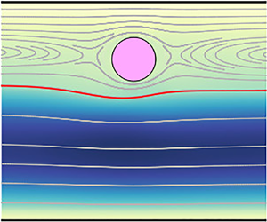
Figures 9 and 10 show the spatial evolution of the interface deformation  $g=\varGamma (x)-\varGamma _{L/2}$ for different capillary numbers. In the limit $Ca^{-1} \gg 1$, the deformation of the interface is anti-symmetrical with respect to the particle and the amplitude of the deformation becomes smaller as the surface tension increases. In contrast, in the limit of small surface tension $Ca^{-1} \ll 1$, the amplitude of the interface deformation is large, of the order of the radius of the particle, with the interface adopting a nearly symmetric shape.

Figure 10. Spatial evolution of the interface deformation  $g/d$ with the capillary number for $Re=0$, $\xi =0.75$ and (a,b) $\mu _{1}/\mu _{2}=2$, $\eta = 0.80$ and (c,d) $\mu _{1}/\mu _{2}=0.50$, $\eta = 0.50$.
Amplitude and symmetry of the interface deformation are quantified by calculating  $g_0= g|_{x=0}$ and $g_{x0}= {\rm d}g/{\rm d}\kern0.7pt x |_{x=0}$, with $g_{x0}=0$ and $g_{x0} \ne 0$ indicating a symmetrical and anti-symmetrical interface deformation, respectively. The functions $g_0$ and $g_{x0}$ are plotted in figure 11 as a function of the position $x$ and of the capillary number with the particle at $\xi =0.75$ moving in the less- $\mu _1/\mu _2=2$ or more-viscous $\mu _1/\mu _2=0.5$ fluid. In both figures, we observed that the solution slowly evolves to achieve $g_{x0} \ll 1$ for extreme values of the capillary number, either because the amplitude of the deformation is small $g \ll 1$ ( $Ca^{-1} \gg 1$) or because the interface becomes nearly symmetrical ( $Ca^{-1} \ll 1$), even when the amplitude of the deformation approaches its maximum value. To plot these figures, we chose the values of $\mu _1/\mu _2$ that maximise the values of $\eta$ at which the interface remains stable in the limit of small surface tension (Yiantsios & Higgins Reference Yiantsios and Higgins1988).

Figure 11. Influence of the inverse of the capillary number  $Ca^{-1}$ on the interface deformation $g_{0}$ and symmetry parameter $g_{x0}$ at $x=0$ for different values of $\eta$ (indicated in the figure), $\xi =0.75$ and (a,c) $\mu _{1}/\mu _{2} = 2$ and (b,d) $\mu _{1}/\mu _{2} = 0.50$.
The magnitude of the computed force  $f$ is similar when the capillary number achieves very large or very small values. To explore the influence of the interface symmetry on the vertical force we plotted in figure 12 the ratio $f/g_{x0}$ versus the capillary number. This figure show that the transverse force is proportional to the symmetry factor $g_{x0}$ in almost the whole range of capillary numbers and becomes independent of $Ca^{-1}$ for extreme values of the surface tension. The main difference is that $f/g_{x0}$ is independent of $L$ for small capillary number but changes with $L$ in the limit $Ca^{-1} \gg 1$, aspect that will be explored in the following section. To understand the relevance of the symmetry of the interface on the vertical force, we decomposed the function $g$ in its symmetrical and anti-symmetrical components $g= g_a + g_s$, defined as $g_s=(g(x)+g(-x))/2$ and $g_a=(g(x)-g(-x))/2$. Figure 12 depicts the anti-symmetrical component $g_a$ of the interface deformation for $Ca^{-1}=0.01$ and $Ca^{-1}=10^4$. In both limits, the order of magnitude of $g_a$ is similar and $g=g_a$ only in the limit $Ca^{-1} \gg 1$, as can be easily checked by comparing figures 9(d) and 12(d). In addition, from figure 12(a) we confirm that the ratio $f/g_{x0}$ becomes constant at large and small values of $Ca$, revealing that both the anti-symmetric part of the interface deformation $g_{x0}$ and the vertical force $f$ scale identically with $Ca$. On the other hand, the symmetric part of the deformation varies differently with $Ca$, as shown in figure 11, and does not contribute to the value of $f$.
$f$.

Figure 12. (a) Evolution of the ratio  $f/g_{x0}$ with the inverse of the capillary number $Ca^{-1}$ for $\mu _{1}/\mu _{2} = 0.50$, $\eta = 0.50$, $\xi = 0.75$ and several inter-particle distances $L$ (values indicated in the figure). On the right panels, we included the anti-symmetrical component of the interface profiles $g_a=(g(x)-g(-x))/2$ calculated for $L=5$ for (b) $Ca^{-1} = 10^{-2}$, (c) $Ca^{-1} = 10^{1.5}$ and (d) $Ca^{-1} = 10^{4}$.
In both limits, the ratio  $f/g_{x0}$ changes only for order-unity values of the capillary number, when the anti-symmetric component of the interface deformation $g_a$ evolves from the asymptotic shape observed at $Ca^{-1} \ll 1$, illustrated in figure 12(b), to the shape of the interface adopted in the limit $Ca^{-1} \ll 1$ depicted in figure 12(b).
4.2. The limit of small surface tension $Ca^{-1} \ll 1$: accuracy of the linear approximation

As suggested by figure 8, the capillary regime  $Ca^{-1} \ll 1$ can be described by considering the expansion $\psi =\psi _0 + Ca^{-1} \psi _{-1}+O( Ca^{-2})$, with $\psi _{j}$ representing any of the dependent variables $p_i$, $\boldsymbol {v}_i$, $V$ and $\varOmega$. As explained in the Appendix A, we also consider small regular perturbations $\delta = Ca^{-1} \delta _{-1}(x)+ O(Ca^{-2})$ normal to the unperturbed interface $\varGamma _0$ so that the coordinates of the perturbed surface $\varGamma '$ can be written as $\boldsymbol {x}'= \boldsymbol {x} +\delta \boldsymbol {n}$ with $\boldsymbol {x}' \in \varGamma '$ and $x \in \varGamma _0$. Considering that $Re=0$ and introducing this expansion in the Navier–Stokes equations, we obtain
 $$\begin{gather} \boldsymbol{\nabla}\boldsymbol{\cdot}\boldsymbol{v}_{i,0} =0 \quad \text{and}\quad 0 = \boldsymbol{\nabla}\boldsymbol{\cdot}\boldsymbol{\hat{\boldsymbol{T}}}_{i,0}, \end{gather}$$
 $$\begin{gather}\boldsymbol{\nabla}\boldsymbol{\cdot}\boldsymbol{v}_{i,-1} =0 \quad \text{and} \quad 0 =\boldsymbol{\nabla}\boldsymbol{\cdot}\boldsymbol{\hat{\boldsymbol{T}}}_{i,-1}. \end{gather}$$
Periodicity and non-slip conditions are imposed at  $x=\pm L/2$ and $y=0$ and $y=1$. To impose the boundary conditions at the perturbed interface $\varGamma ^{\prime }$, we use the methodology originally described by Rivero-Rodriguez et al. (Reference Rivero-Rodriguez, Perez-Saborid and Scheid2018), that we summarised in the Appendix A for the sake of completeness. Consequently, the condition of non-penetrability and continuity of velocity at the interface is then given by
 $$\begin{gather} \boldsymbol{n}\boldsymbol{\cdot}\boldsymbol{v}_{2,0} = 0, \quad [\boldsymbol{v}_{0}] =\boldsymbol{0}, \end{gather}$$
 $$\begin{gather}\boldsymbol{n}\boldsymbol{\cdot}\boldsymbol{v}_{2,-1} - {\boldsymbol{D}_{S}}\boldsymbol{\cdot}(\delta_{{-}1} \boldsymbol{v}_{2,0}) = 0, \quad {[\boldsymbol{v}_{{-}1}] + \delta_{{-}1} \boldsymbol{n}\boldsymbol{\cdot}\boldsymbol{\nabla} ([\boldsymbol{v}_{0}])=\boldsymbol{0}}. \end{gather}$$
The stress balance at the interface is now written as
 $$\begin{gather} \boldsymbol{n}\boldsymbol{\cdot}\left[\hat{\boldsymbol{T}}_{0}\right] = 0, \end{gather}$$
 $$\begin{gather}\boldsymbol{n}\boldsymbol{\cdot}\left[\hat{\boldsymbol{T}}_{{-}1}\right] -{\boldsymbol{D}_{S}}\boldsymbol{\cdot}\left( \delta_{{-}1} \left[\hat{\boldsymbol{T}}_{0}\right] \right) = {\boldsymbol{D}_{S}} 1, \end{gather}$$
with  $\boldsymbol {n}$ representing the normal vector to the unperturbed interface $\varGamma _0$, $\boldsymbol {\nabla }_S \psi =(\boldsymbol{\mathsf{I}}-\boldsymbol {n}\boldsymbol {n})\boldsymbol {\cdot }\boldsymbol {\nabla } \psi$ and the differential operator ${\boldsymbol {D}_{S}} \psi = -(\boldsymbol {n} \boldsymbol {\nabla }\ {\boldsymbol{\cdot} }\ \boldsymbol {n}) \psi + \boldsymbol {\nabla }_S \psi$. The rotational velocity is computed considering non-slip conditions (2.7) and equilibrium of moments (2.8). The terminal velocity is obtained imposing the equilibrium in $x$ direction given by (2.6).
Once the first order of the solution is obtained, we compute the first correction for the force  $k_3=f \,Ca$ using (2.11). The results of that calculations are compared in figure 13 with the results of the integration of the full problem specified in (2.1)–(2.9) with $Re=0$ and $Ca^{-1} \ll 1$ but non-zero. The linear approximation of the solution works fairly well for order-unity values of the capillary number $Ca^{-1}=1$ when the particle is in the less-viscous fluid $\mu _1/\mu _2=2$, but rapidly worsens for larger surface tensions giving wrong predictions for up to 35 % when $Ca =3.16$. In the limit of small surface tension, the linear approximation gives an accurate prediction of the force for relatively large capillary numbers $Ca^{-1}=10^{-0.5}$ as long as the particle is not very close to the interface. In that region, the validity of the linear approximation is confined to the small values of the inverse of the capillary number $Ca^{-1} \ll 1$ hypothesised in the derivation of this section.

Figure 13. Comparison of the force  $f\,Ca$ obtained in the linear limit $Ca^{-1} \ll 1$ (black solid lines) with the computations using small but finite values of $Ca^{-1}$ (indicated in the figure): (a) $\mu _{1}/\mu _{2} = 2$, $\eta = 0.80$ and (b) $\mu _{1}/\mu _{2} = 0.50$, $\eta = 0.50$.
As the viscosity ratio  $\mu _1/\mu _2$ increases, the flow rate in the bottom layer decreases proportionally and, in the limit of very high-viscosity ratios, the continuity of velocities at the interface approximates to a non-slip boundary condition. At sufficiently high values of the viscosity ratio, both the symmetrical and anti-symmetrical parts of the interface deformation become small $g \sim (\mu _1/\mu _2)^{-1}$ and $g_{x0} \sim (\mu _1/\mu _2)^{-2}$ and, consequently, the external body force becomes $f \sim (\mu _1/\mu _2)^{-2} \ll 1$. This result, which can be also demonstrated by deriving the asymptotic linear solution in the limit $\mu _{1}/\mu _{2} \gg 1$, reveals that, in this limit, the particles would be at equilibrium without the need of an external body force regardless of the particles position. Interestingly, the viscous layer would behave as a passive fluid with negligible deformation.
4.3. Large surface tension $Ca^{-1} \gg 1$: influence of the capillary number on the minimum inter-particle distance $L$


Surface tension has a stabilising effect and, therefore, the range of the parameters within which the interface is unstable asymptotically vanish in the limit  $Ca^{-1} \gg 1$ (Yiantsios & Higgins Reference Yiantsios and Higgins1988). Consequently, we can illustrate the evolution of the flow variables and the force $f$ with the capillary number and the distance between particles $L$ in a much wider range of parameter $\eta$ and $\mu _{1}/\mu _{2}$ than in the limit $Ca^{-1} \ll 1$.
At large values of  $Ca^{-1}$, figure 9 shows a sudden change in the asymptotic behaviour of the force, that becomes $f/Ca=k_1$, with $k_1=k_1(\eta,\xi,L)$ a constant value that will be calculated in the following. Black dots in this figure indicate the capillary number at which this occurs $Ca^{-1} =(Ca^{-1})^*$, being $(Ca^{-1})^*$ a critical value of the capillary number that will be computed below.
The presence of the particle near the interface induces a deformation whose characteristic length is  $\lambda =x_{max}-x_{min}$, defined as the difference between the longitudinal positions $x_{max}$ and $x_{min}$ at which $g=\bar {g}$, with the average deformation of the interface defined as $\bar {g} =L^{-1} \int _{-L/2}^{L/2} g \,{{\rm d}\kern0.06em x}$. The dependence of $\lambda$ with $Ca^{-1}$ is depicted in the right panels of figure 9 and in figure 14 for several inter-particle distances. As we anticipated, $\lambda$ is independent of the capillary number for $Ca^{-1} < 0.1$. The small dependence of $\lambda$ with the inter-particle distance is explained by the changes observed in the symmetrical part of the deformation $g_s$ with $L$. As shown in figure 9, the force $f$ is independent of $L$ in the limit $Ca^{-1} \ll 1$ evidencing, again, that the anti-symmetrical part of the interface deformation $g_a$ is the only factor responsible for the vertical force exerted on the particle.

Figure 14. (a) Influence of the inter-particle distance on the region of influence of the deformation  $\lambda$. The black dots indicate the beginning of the linear regime when $Ca^{-1}=(Ca^{-1})^*$. (b) Variation of the computed values of $(Ca^{-1})^*$ with $L$ (Blue solid line). The black, dashed line corresponds to the fitted curve $y= 1.55 L^{2.98}$. All calculations are carried out for $\mu _{1}/\mu _{2} = 0.50$, $\eta = 0.50$ and $\xi = 0.75$.
In the transition region  $Ca^{-1} < (Ca^{-1})^*$, the length $\lambda$ is determined by the surface tension and remains smaller than the inter-particle distance $L$. Therefore, the surface tension introduces a new length scale that determines the asymptotic behaviour of both the flow parameters and the transverse force, with the latter following a generic dependence on the form $f/Ca=k_2 Ca^{-n}$. The exponent $n$ is given in table 1 for different values of $\xi$, $\eta$ and $\mu _1/\mu _2$. When the surface tension increases above the threshold value $Ca^{-1}>(Ca^{-1})^*$, the length $\lambda$ becomes of the order of the inter-particle distance $L/2$ and the asymptotic behaviour of the force becomes $f/Ca=k_1$. To illustrate this, we included in the right panels of figure 9 the influence of the capillary number on the shape of the interface. In the limit of small surface tension $Ca^{-1}=10^{-2}$, the interface deforms symmetrically around the particle (figure 9a) and the region of influence of the particle on the interface is small. As we increase the surface tension, $\lambda$ becomes longer until it does not fit between two consecutive particles. In the limit $Ca^{-1} \gg 1$, the computations show a anti-symmetrical deformation (figure 9c) with $\lambda =L/2$. The critical value of the capillary number $(Ca^{-1})^*$ above which $\lambda =L/2$ and the vertical force enters in the linear regime is calculated by increasing the surface tension and monitoring when the force becomes constant $f/Ca=k_1$. The black symbols in figures 9, 12 and 14 indicate when $Ca^{-1}= (Ca^{-1})^*$ and show that the linear dependence of $f$ with $Ca$ starts only when $\lambda \simeq L/2$. The right panel of figure 14 shows that the critical capillary number scales with the inter-particle distance as $(Ca^{-1})^* \propto L^{-\alpha }$, being $\alpha =-3$ for $\mu _{1}/\mu _{2} = 0.50$, $\eta = 0.50$ and $\xi = 0.75$. Additional values of the exponent $\alpha$ are included in table 1 for $\mu =0.5$, $\mu =2$ and different particle $\xi$ and interface $\eta$ locations.
Table 1. Variation of the length scaling factor  $\alpha$ and the transition regime slope $n$ with the interface $\eta$ and particle $\xi$ position for $\mu _{1}/\mu _{2}=0.5$ and $\mu _{1}/\mu _{2}=2$.

As indicated previously, when the length of the interface deformation is longer than the inter-particle distance  $\lambda \geqslant L/2$, the problem reaches a linear regime in which all variables can be expanded in terms of the capillary number on the form $\psi =\psi _0 + Ca\,\psi _1+ O(Ca^2)$. This expansion fails when the length of the deformation is smaller than the inter-particle distance $\lambda < L/2$ and $\lambda$ becomes the relevant characteristic length. In this case, the dependence of the variables with the capillary number should be written in the form $\psi =\psi _0 + Ca^{1-n}\,\psi _1+ O(Ca^{2(1-n)})$, with $n \ne 1$ determined from the numerical solution in § 4.3.1.
4.3.1. Asymptotic solution in the limit $Ca^{-1}<(Ca^{-1})^*$ and $\lambda < L/2$


In this intermediate region, all variables can be expanded in terms of the capillary number as  $\psi = \psi _0 + Ca^{1-n} \psi _1 + \dots$ with $f=Ca^{1-n} k_2+ O(Ca^{2(1-n)})$. To determine the value of the exponent $n$, we plot in figure 15 the value of the scaled force $f/(k_1 Ca)$ in terms of $Ca^{-1} L^\alpha$ so that all curves converge at $f/(k_1 Ca)=1$ when $Ca^{-1} \geqslant (Ca^{-1})^*$, with the value of the exponent $\alpha$ given in table 1 as a function of $\eta$ and $\xi$. For $\mu _1/\mu _2=0.5$, $\eta =0.5$ and any inter-particle distance $L$, the slope of the curves in the intermediary region $Ca^{-1} < (Ca^{-1})^*$ determines the value of the exponent $n=1/3$. This value is independent of the interface location $\eta$ and depends weakly on the particles position $\xi$, as indicated in table 1.

Figure 15. Evolution of the force  $f/(Ca \,k_1)$ for $\mu _{1}/\mu _{2} = 0.50$, $\eta = 0.50$ and (a) $\xi = 0.75$ and (b) $\xi = 0.25$. Solid lines for repulsive (positive) force $f$ and dashed lines for attractive (negative) values with respect to the interface.
The position of the particle clearly affects the value of the force  $f$, as shown in figure 15. In contrast to what was observed before in figure 4 in the limit $Ca=0$, near the wall $\xi =0.75$ the fluid exerts a positive force $f$ on the particle. A change on the sign of the force is observed as the particle approaches the interface $\xi =0.25$ at intermediate values of the capillary number when $L>5$, as shown with dashed lines in the curves plotted in figure 15b) and in figure 16. With this combination of parameters, the force exerted on the particle $f$ is negative and the particle is pushed towards the interface. The negative value of $f$ is a direct consequence of the shape of the interface and the amplitude of the interface deformation, as can be checked by looking at figure 16b). The sign of the force $f$ remains unchanged for larger surface tensions, an effect that anticipates a natural tendency of the particle to migrate towards the interface that can be used to design passive filters.

Figure 16. Evolution of (a) the force  $f/(Ca)$ and (b) the derivative at $x=0$ of the interface deformation $g_{x}$ for $\mu _{1}/\mu _{2} = 0.50$, $\eta = 0.50$, $\xi = 0.25$. The insets show in detail the region where the sign of (a) the force $f$ and (b) $g_{x0}$ changes from positive to negative. In (b) the evolution of the deformation at the centre of the particle $x=0$, $g_{0}/d$ with $Ca^{-1}$ is illustrated in the upper inset. Solid lines for values corresponding to repulsive (positive) force $f$ and dashed lines for attractive (negative) values of $f$ with respect to the interface.
4.3.2. Asymptotic solution in the limit $Ca^{-1}>(Ca^{-1})^*$ and $\lambda > L/2$


In the pure capillary regime, the system of equations can be regularly expanded as  $\psi = \psi _0+Ca \,\psi _1 + O(Ca^2)$, with $\psi =(\hat {p}_i, \boldsymbol {v}_i,V,\varOmega, f, \Delta p$). The perturbation of the interface $\varGamma _0$ is expressed in terms of an infinitesimal normal displacement $\boldsymbol {\delta }= \delta \boldsymbol {n}$ with $\delta =\delta _1 Ca + \delta _2 Ca^2 + {O}(Ca^3)$.
The resulting expansion of the Navier–Stokes equations up to first order yield,
 $$\begin{gather} \boldsymbol{\nabla}\boldsymbol{\cdot}\boldsymbol{v}_{i,0} =0 \quad \text{and} \quad 0 = \boldsymbol{\nabla}\boldsymbol{\cdot}\hat{\boldsymbol{T}}_{i,0}, \end{gather}$$
 $$\begin{gather}\boldsymbol{\nabla}\boldsymbol{\cdot}\boldsymbol{v}_{i,1} =0 \quad \text{and} \quad 0 = \boldsymbol{\nabla}\boldsymbol{\cdot}\hat{\boldsymbol{T}}_{i,1}, \end{gather}$$
at the unperturbed surface  $\varGamma _0$. To compute the terms of the expansion of the terminal and rotational velocity we imposed, as before, equilibrium in $x$ direction (2.6), non-slip (2.7) and the zero-torque condition (2.8) at the particle at every order of the solution. The continuity of velocity and non-penetrability conditions are enforced at the interface
 $$\begin{gather} \boldsymbol{n}\boldsymbol{\cdot}\boldsymbol{v}_{2,0} = 0, \quad [\boldsymbol{v}_{0}]=\boldsymbol{0} \end{gather}$$
 $$\begin{gather}\boldsymbol{n}\boldsymbol{\cdot}\boldsymbol{v}_{2,1} - {\boldsymbol{D}_{S}}\boldsymbol{\cdot}(\delta_1 \boldsymbol{v}_{2,0}) = 0, \quad {[\boldsymbol{v}_{1}] + \delta_1 \boldsymbol{n}\boldsymbol{\cdot}\boldsymbol{\nabla} ([\boldsymbol{v}_{0}])=\boldsymbol{0}}. \end{gather}$$
The first-order solution  $Ca=0$ of the stress jump condition gives the unperturbed surface $\varGamma _0=\eta (1-d)$ while the first- and second-order perturbations yield
 $$\begin{gather} \boldsymbol{n}\boldsymbol{\cdot}\left[\hat{\boldsymbol{T}}_{0}\right] = {\boldsymbol{D}_{S}}\boldsymbol{\cdot}\boldsymbol{\mathsf{B}}_{\boldsymbol{1}} \end{gather}$$
 $$\begin{gather}\boldsymbol{n}\boldsymbol{\cdot}\left[\hat{\boldsymbol{T}}_{1}\right] - {\boldsymbol{D}_{S}}\boldsymbol{\cdot}\left( \delta_1 \left[\hat{\boldsymbol{T}}_{0}\right] \right) = {\boldsymbol{D}_{S}}\boldsymbol{\cdot}\boldsymbol{\mathsf{B}}_{\boldsymbol{2}}, \end{gather}$$
with the rotation tensor  $\boldsymbol{\mathsf{B}}=Ca \,\boldsymbol{\mathsf{B}}_1 + Ca^2 \boldsymbol{\mathsf{B}}_2 + O(Ca^3)$ defined such that $\boldsymbol{\mathsf{B}}=\boldsymbol {n}_{S0} \boldsymbol {n}_{Sp}$, with $\boldsymbol {n}_{S0}$ and $\boldsymbol {n}_{Sp}$ the tangential vectors to the unperturbed $\varGamma _0$ and perturbed interface $\varGamma ^{\prime }$, as shown in the Appendix A. In 2-D Cartesian coordinates, the rotation tensor $\boldsymbol{\mathsf{B}}=\boldsymbol {e}_x \boldsymbol {n}_{Sp}$ and $\boldsymbol {n}_{Sp} = (\boldsymbol {e}_{x}-\delta _x \,\boldsymbol {n})/| \boldsymbol {e}_{x}-\delta _x \,\boldsymbol {n} |$, with $\delta _x={\rm d}\delta /{{\rm d}\kern0.06em x}$. Then, the right-hand side of (4.11) and (4.12) can be written using the first two orders of the expansion giving ${\boldsymbol {D}_{S}}\boldsymbol {\cdot }\boldsymbol{\mathsf{B}}_1= \delta _{xx,1} \boldsymbol {e}_y$ and ${\boldsymbol {D}_{S}}\boldsymbol {\cdot }\boldsymbol{\mathsf{B}}_2= \delta _{xx,2} \boldsymbol {e}_y - \delta _{x,1} \delta _{xx,1} \boldsymbol {e}_x$, with $\delta _{xx}={\rm d}^2\delta /{{\rm d}\kern0.06em x}^2$. In addition, non-slip conditions are imposed at the walls $y=0$ and $y=1$ and periodic boundary conditions far from the particle $x =\pm L/2$.
Once the rest of the variables are computed, the first order of the force  $f= Ca \ k_1 + O(Ca^2)$ is determined numerically integrating (2.11). For $L=40$, figure 9 anticipates that the linear regime is achieved for $Ca^{-1}=(Ca^{-1})^* = 10^{5}$. To check this point, we compared the force $f/Ca$ obtained using the linear approximation with the numerical results obtained integrating the full problem (2.1)–(2.11) in figure 17. As expected, both solutions are indistinguishable for $Ca^{-1}>10^5$.

Figure 17. Computed vertical force  $f/Ca$ in terms of the particle position for several capillary numbers $Ca$, with (a) $\mu _{1}/\mu _{2}= 2$, $\eta = 0.80$ and (b) $\mu _{1}/\mu _{2}=0.50$, $\eta = 0.50$. In all computations $L=40$.
Once the linear solution is validated, we computed the variation of the force  $f/Ca$ with the position of the particle in the channel for different viscosity ratios $\mu _1/\mu _2$ and interface location. The results, plotted in figure 18, show only one neutral equilibrium position for $\mu _1/\mu _2<1$ when the interface is at $\eta =0.5$ but, unlike the pure inertial case presented previously, is unstable. One or three equilibrium positions are found when $\mu _1/\mu _2>1$ but they only remain stable when the particle is far from both the interface or the wall, again a behaviour that is the opposite to what we found in the pure inertial case. A similar trend is observed at low values of $\xi$ once we modify the location of the interface keeping $\mu _1/\mu _2=0.5$. When $\eta >0.5$, we find none or one unstable equilibrium position when the particle is near to the interface. Up to three equilibrium positions $f=0$, two of them unstable, are found when $\eta <0.5$. Again, the only stable equilibrium position is found when the particle is halfway between the wall and the interface.

Figure 18. Effect of the position of the particle  $\xi$ on the force $f/Ca$ in the linear regime $Ca^{-1} > (Ca^{-1})^*$ with $L=40$ for different values (a) of the viscosity ratio $\mu _{1}/\mu _{2}$ with $\eta =0.50$ and (b) of the interface position $\eta$ with $\mu _{1}/\mu _{2}=0.50$.
The isocontours of the computed force  $f/Ca$ are plotted in figure 19 in the $\eta$– $\xi$ parametric space. The asymptotic equilibrium positions $f=0$ of the particle are plotted using black thick curves. The isolines $\partial f/\partial \xi =0$ in which the stability behaviour of the equilibrium position shifts from unstable to stable and vice versa are included in dashed lines. As shown in this figure, up to three equilibrium positions can be found in a wide range of values of $\eta$ for both $\mu _1/\mu _2$ larger and smaller than one, with only one of them within the stable region.

Figure 19. Isocontours of the scaled force  $f/Ca$ obtained with the asymptotic solution in the plane $\eta$– $\xi$ for (a) $\mu _{1}/\mu _{2}=2$ and (b) $\mu _{1}/\mu _{2}=0.50$. Solid black lines represent equilibrium positions ( $f/Ca=0$) and dashed black lines indicate stability transition ( $\partial _\xi f/Ca =0$). White solid regions for unstable particle positions, gray regions for stable. The colour bar is piecewise linear, being the linear sections and is corresponding level step: ${\pm }6428$ for $|f/Ca| \geqslant 10\,000$, ${\pm }500$ for $500<|f/Ca|<5000$ and ${\pm }100$ for $|f/Ca|<250$.
A steep gradient on the transverse force  $f$ is observed in figure 19 when we modify the position of the interface $\eta$ keeping $\xi$ constant. This figure reveals a variation of the vertical force of several orders of magnitude, including a sign change that indicates that the particle is pushed either away or towards the interface depending on the location of the interface. This is clearly opposed to what is observed in the pure inertial regime included in figure 5, in which the force $f$ is only weakly dependent on the position of the interface once the position of the particle $\xi$ is set. Similarly, for intermediate values of the interface position eta, the value of the transverse force also varies dramatically with the particle position, being negative (attractive) for values close to the interface and positive (repulsive) when the particle is close to the upper wall.
5. Conclusions
Using a finite-element method combined with the ALE method we have studied the dynamics of a train of solid particles separated by a distance  $L$ moving near the interface of two co-flowing immiscible liquids. The presence of the interface introduces a new force that plays a crucial role in determining the equilibrium position of the particles.
The first part of the work considered a non-deformable interface corresponding to the limit of infinitely large surface tension  $Ca = 0$ with small, but finite, Reynolds number. In this limit, we found that the force is weakly dependent on the position of the interface but its sign varies significantly with the position of the particle. Our calculation showed that the particle is pushed towards the interface (wall) when it is near the wall (interface). Up to three neutral equilibrium positions $f=0$, two of them stable, are found when the particle is embedded in the less-viscous fluid. When the particle travels in the more-viscous fluid, a unique, neutral stable equilibrium position was found regardless of the particle or the interface positions. The asymptotic linear solution for the flow variables $\psi = \psi _0 + Re \,\psi _1$ found in the limit $Re \ll 1$ remains valid for values of the Reynolds number as large as $Re=60$ when $\mu _1/\mu _2 > 1$. This is not the case when $\mu _1/\mu _2 < 1$ as nonlinear effects become relevant even when $Re=0.1$ due to the greater relative importance of the convective terms in fluid 1.
In the pure capillary regime  $Re=0$, we computed the force necessary to keep the particle at a given vertical location $\xi$ in a wide range of capillary numbers $10^{-4} < Ca^{-1} < 10^{6}$. The results identified three different regimes depending of the value of the capillary number. In the limit $Ca^{-1} \ll 1$, the amplitude of the interface deformation induced by the particle is large, comparable to its diameter, but its influence is limited to a small region upstream and downstream of the particle. In this limit, all variables can be expanded asymptotically as $\psi =\psi _0 + Ca^{-1} \psi _1$ with the first correction of the force written as $Ca \,f=k_3$ and $k_3$ a constant that depends on both $\eta$ and $\xi$. This linear approximation remains valid up to values of the capillary number of order unity as long as $\mu _1/\mu _2 >1$. As in the inertial case, nonlinear effects emerge at much lower values of the capillary number when $\mu _1/\mu _2<1$.
The limit of very large surface tension  $Ca^{-1} \gg 1$ turns out to be more intricate. As expected, the amplitude of the interface deformation reduces with increasing capillary number and becomes much smaller than the particle diameter. Nevertheless, the region of influence of the particle $\lambda$ becomes wider as the surface tension increases, becoming of the order of the inter-particle distance for capillary numbers above a critical value $(Ca^{-1})^*$. Above this value, the asymptotic behaviour of the flow variables become linear with the inverse of the capillary number so that $\psi =\psi _0 + Ca \,\psi _1$ and $f/Ca=k_1$, with $k_1$ a constant that depends on both the location of the interface $\eta$ and the particle $\xi$. Below that threshold value $Ca^{-1} < (Ca^{-1})^*$, the relevant characteristic length becomes $\lambda$ instead of $L$, modifying the asymptotic behaviour of the solution that adopts an asymptotic expansion on the form $\psi =\psi _0 + Ca^{1-n} \psi _1$ with $f/Ca=k_2 Ca^{-n}$, with $k_2$ and $n$ computed numerically in terms of $\eta$ and $\xi$.
In the pure capillary regime  $Re=0$, the anti-symmetrical component of the interface deformation is responsible for the vertical forces $f$ exerted on the particle. The position of both the interface $\eta$ and the particle $\xi$ control the sign of $f$. Once the position of the interface $\eta$ is determined, the particle is pushed towards the interface (wall) when the particle is placed near the interface (wall), a result that is opposed to what was observed in the pure inertial regime when the interface was non-deformable $Ca=0$.
Funding
This work was funded by the Agencia Estatal de Investigación of Spain PID2019-108592RB-C41/ AEI/10.13039/501100011033. D.R.-M. acknowledges the support of an FPI predoctoral fellowship (BES-2016-078629). APC funded by Universidad Carlos III de Madrid (Read and Publish Carlos III University of Madrid 2022).
Declaration of interest
The authors report no conflict of interest.
Appendix A. Interface perturbation
In order to perturb the interface separating both fluids, we applied a normal differential displacement  $\boldsymbol {\delta }=\delta (\boldsymbol {x} ) \boldsymbol {n}$ that creates a volume $\mathcal {V}$ as a result of the displacement of the interface from $\varGamma _0$ to its perturbed position $\varGamma '$, as sketched in figure 20.

Figure 20. Fluid volume obtained when the interface  $\varGamma$ is perturbed with a normal perturbation $\boldsymbol {\delta }=\delta \boldsymbol {n}$ to form the perturbed interface $\varGamma '$.
The boundary conditions at the interface (2.9) and (2.10a,b) need to be evaluated at the perturbed interface  $\varGamma '$ to properly account for the displacement $\boldsymbol {\delta }$ during the asymptotic expansions carried out in §§ 4.2 and 4.3. The position of the perturbed interface $\varGamma '$ is unknown and will be obtained as part of the calculation process. Consequently, to evaluate (2.9) and (2.10a,b) we followed the methodology developed by Rivero-Rodriguez et al. (Reference Rivero-Rodriguez, Perez-Saborid and Scheid2018) to write the boundary conditions at the unperturbed surface $\varGamma _0$. To do so, we start by subtracting the momentum equations (2.2) written for fluid 2 and fluid 1. Integrating the resulting expression in the volume $\mathcal {V}$ and using Gauss's theorem to transform the volume integral into surface integrals, we obtained
 \begin{equation} -\int_{\varGamma_0} \boldsymbol{n}\boldsymbol{\cdot}[\hat{\boldsymbol{T}}] \,\mathrm{d}\varSigma + \int_{\varGamma'} \boldsymbol{n}'\boldsymbol{\cdot}[\hat{\boldsymbol{T}}] \,\mathrm{d}\varSigma + \int_{C_0} \delta [\hat{\boldsymbol{T}}]\boldsymbol{\cdot}\boldsymbol{n}_{S0} \,\mathrm{d} l = \int_{\mathcal{V}} [\boldsymbol{\mathcal{F}}] \,{\rm d}V , \end{equation}
with  $\boldsymbol {\mathcal {F}}_i=Re\,\boldsymbol {v}_i\boldsymbol {\cdot }\boldsymbol {\nabla } \boldsymbol {v}_i$ and $C_0=\partial \varGamma _0$ so that $\varGamma _l=\int _{C_0} \delta \,{\rm d}l$ is the lateral surface of the $\mathcal {V}$. The line integral in the left hand side of previous equation can be transformed to a surface integral, giving
 \begin{equation} \int_{C_0} \delta [\hat{\boldsymbol{T}}]\boldsymbol{\cdot}\boldsymbol{n}_{S0} \,{\rm d}l = \int_{\varGamma_0} {\boldsymbol{D}_{S}}\boldsymbol{\cdot}(\delta [\hat{\boldsymbol{T}}]) \,\mathrm{d}\varSigma , \end{equation}
where  ${\boldsymbol {D}_{S}}$ is the differential operator ${\boldsymbol {D}_{S}} \theta = \boldsymbol {\nabla }_S \theta -(\boldsymbol {n}\boldsymbol {\nabla }_{S}\boldsymbol {\cdot }\boldsymbol {n} ) \theta$. The volume integral on the right-hand side of (A1) can be expressed as $\int _{\mathcal {V}} [\boldsymbol {\mathcal {F}}] \,{\rm d}V=\int _{\varGamma _0} \delta [\boldsymbol {\mathcal {F}}] \,\mathrm {d}\varSigma$ and (A1) can be written as
 \begin{equation} \int_{\varGamma'} \boldsymbol{n}'\boldsymbol{\cdot}[\hat{\boldsymbol{T}}] \,\mathrm{d}\varSigma = \int_{\varGamma_0} \left[\boldsymbol{n}\boldsymbol{\cdot}[\hat{\boldsymbol{T}}] - {\boldsymbol{D}_{S}}\boldsymbol{\cdot}(\delta [\hat{\boldsymbol{T}}]) + \delta [\boldsymbol{\mathcal{F}}] \right] {\rm d}\varSigma . \end{equation}
Next, substituting the boundary condition (2.10a,b) in (A3), it yields
 \begin{equation} \int_{\varGamma'} Ca^{{-}1}D_S1 \,\mathrm{d}\varSigma = \int_{\varGamma_0} \left[\boldsymbol{n}\boldsymbol{\cdot}[\hat{\boldsymbol{T}}] - {\boldsymbol{D}_{S}}\boldsymbol{\cdot}(\delta [\hat{\boldsymbol{T}}]) + \delta [\boldsymbol{\mathcal{F}}] \right] {\rm d}\varSigma . \end{equation}
The differential operator  ${\boldsymbol {D}_{S}}$ on the left-hand side of (A4) can also be perturbed to facilitate its evaluation. Following Rivero-Rodriguez et al. (Reference Rivero-Rodriguez, Perez-Saborid and Scheid2018), and using (A2), for a perturbation $\delta$ normal to $\varGamma$ we can write
 \begin{equation} \int_{\varGamma'} {\boldsymbol{D}_{S}} \phi \,\mathrm{d}\varSigma = \int_{C'} \boldsymbol{n}'_{S}\phi \,{\rm d}\boldsymbol{l}= \int_{\varGamma_0} {\boldsymbol{D}_{S}}\boldsymbol{\cdot}\left( \boldsymbol{\mathsf{B}} \phi \right) {\rm d}\varSigma , \end{equation}
with the rotation tensor  $\boldsymbol{\mathsf{B}}$ defined such that $\boldsymbol{\mathsf{B}}=\boldsymbol {n}_{S0} \boldsymbol {n}'_{S}$. Using this result, (A4) finally reduces to
 \begin{equation} \boldsymbol{n}\boldsymbol{\cdot}\left[\hat{\boldsymbol{T}} \right] - {\boldsymbol{D}_{S}}\boldsymbol{\cdot}\left(\delta \left[\hat{\boldsymbol{T}} \right] \right) + \delta \left[\boldsymbol{\mathcal{F}}\right] =Ca^{{-}1} {\boldsymbol{D}_{S}}\boldsymbol{\cdot}\boldsymbol{\mathsf{B}} \quad \textrm{at} \ \varGamma_0 , \end{equation}
where the tensor  $\boldsymbol{\mathsf{B}}$ needs to be determined in each particular case.
By the same token, to enforce the kinematic condition (2.9), we use the same procedure than before and we integrate the continuity equation for the fluid 2 in the created volume  $\mathcal {V}$, to write
 \begin{equation} -\int_{\varGamma_0} \boldsymbol{n}\boldsymbol{\cdot}\boldsymbol{v}_2 \,\mathrm{d}\varSigma +\int_{\varGamma'} \boldsymbol{n}'\boldsymbol{\cdot}\boldsymbol{v}_2 \,\mathrm{d}\varSigma + \int_{C_0} \delta \boldsymbol{v}_2\boldsymbol{\cdot}\boldsymbol{n}_{S0} \,\mathrm{d}\varSigma=0 . \end{equation}
After imposing (2.9) at  $\varGamma '$ and using (A2) with $\delta \boldsymbol {v}_1$ substituting $\delta [\hat {\boldsymbol {T}}]$, it yields
 \begin{equation} \boldsymbol{n}\boldsymbol{\cdot}\boldsymbol{v}_{2} - {\boldsymbol{D}_{S}}\boldsymbol{\cdot}(\delta \boldsymbol{v}_{2})=0 \quad \textrm{at} \ \varGamma_0 .\end{equation}
To impose the continuity of velocity  $[\boldsymbol {v}]=0$ at $\varGamma ^{\prime }$ given in (2.9), we keep the first-order term of the Taylor expansion of the velocity difference to give
 \begin{equation} \left[\boldsymbol{v}\right] +\delta \boldsymbol{n}\boldsymbol{\cdot}\boldsymbol{\nabla}[\boldsymbol{v}] =0 , \end{equation}
evaluated at  $\varGamma _0$. Once the differential displacement $\delta$ is obtained, the perturbed interface $\varGamma '$ can be obtained as $\boldsymbol {x}'=\boldsymbol {x} + \delta \boldsymbol {n}$, where $\boldsymbol {x}' \in \varGamma '$ and $\boldsymbol {x} \in \varGamma _0$.


 Open access