


1. Introduction
Superhydrophobic (SHPo) surfaces have been one of the most popular topics in science and engineering over the last two decades because of their unique potentials, such as hydrodynamic drag reduction (Ou, Perot & Rothstein Reference Ou, Perot and Rothstein2004; Choi & Kim Reference Choi and Kim2006), self-cleaning (Barthlott & Neinhuis Reference Barthlott and Neinhuis1997), anti-icing (Cao et al. Reference Cao, Jones, Sikka, Wu and Gao2009), anti-biofouling (Marmur Reference Marmur2006) and anti-corrosion (Liu et al. Reference Liu, Yin, Chen, Chang and Cheng2007). Among them, drag reduction of watercraft has been cited as a motivating factor in nearly every publication on SHPo surfaces for its global-scale impact on energy saving and environmental protection (Park, Choi & Kim Reference Park, Choi and Kim2021). When a SHPo surface is completely immersed in water, a substantially continuous layer of air, commonly called a plastron (Brocher Reference Brocher1912), may be formed on it and produce a slip boundary that reduces skin friction drag. While all numerical studies over the years (Min & Kim Reference Min and Kim2004; Fukagata, Kasagi & Koumoutsakos Reference Fukagata, Kasagi and Koumoutsakos2006; Martell, Perot & Rothstein Reference Martell, Perot and Rothstein2009; Park, Park & Kim Reference Park, Park and Kim2013; Rastegari & Akhavan Reference Rastegari and Akhavan2015; Im & Lee Reference Im and Lee2017) and many experimental studies in the 2010s (Daniello, Waterhouse & Rothstein Reference Daniello, Waterhouse and Rothstein2009; Bidkar et al. Reference Bidkar, Leblanc, Kulkarni, Bahadur, Ceccio and Perlin2014; Park, Sun & Kim Reference Park, Sun and Kim2014; Gose et al. Reference Gose, Golovin, Boban, Mabry, Tuteja, Perlin and Ceccio2018) have reported a significant drag reduction, successful drag-reduction experiment in fully turbulent flows in open water, which represents the field condition of watercraft, has not been reported until 2020 (Xu et al. Reference Xu, Grabowski, Yu, Kerezyte, Lee, Pfeifer and Kim2020b, Reference Xu, Yu, Kim and Kim2021). These most recent successes have eased the skepticism that had grown against the SHPo drag reduction, after two decades of research without any successful field experiments. Importantly, the successful reports strongly suggested that most of the inconsistent experimental results in the past may have been simply due to the loss or deterioration of the plastron. In other words, the original notion of SHPo drag reduction is valid as far as the plastron remains in a good shape. The tortuous path to the current state of knowledge also indicates how difficult yet important it is to accurately monitor the state of the plastron during experimental studies of SHPo drag reduction, leading to the two-camera observation technique by Yu et al. (Reference Yu, Kiani, Xu and Kim2021). Focusing on longitudinal micro-trench SHPo surfaces, which have been the most effective for drag reduction (Park et al. Reference Park, Choi and Kim2021) and to help the design of SHPo surfaces capable of reducing the drag for watercraft, this paper aims to understand the range of trench geometries that can maintain a pinned or slightly degraded plastron, which has its air–water interfaces pinned or slightly depinned at the top edges over the entire or nearly entire trench length so that much of the pristine slip capability is preserved, in high-speed open-water flows.
Over the years, hydrostatic pressure and air diffusion have been found to affect the plastron stability in stationary (Bobji et al. Reference Bobji, Kumar, Asthana and Govardhan2009; Poetes et al. Reference Poetes, Holtzmann, Franze and Steiner2010; Samaha, Vahedi Tafreshi & Gad-el-Hak Reference Samaha, Vahedi Tafreshi and Gad-el-Hak2012; Lv et al. Reference Lv, Xue, Shi, Lin and Duan2014; Xu, Sun & Kim Reference Xu, Sun and Kim2014) and flowing (Ling et al. Reference Ling, Katz, Fu and Hultmark2017; Kim & Park Reference Kim and Park2019) water. More recently, the shear-driven drainage (Wexler, Jacobi & Stone Reference Wexler, Jacobi and Stone2015; Liu et al. Reference Liu, Wexler, Schönecker and Stone2016), which was developed to understand the loss of infused oil on liquid infused surfaces (LIS) (Wong et al. Reference Wong, Kang, Tang, Smythe, Hatton, Grinthal and Aizenberg2011) caused by the shear in flowing water, has been borrowed to explain the plastron loss on trench SHPo surface in very high shear flows (Xu et al. Reference Xu, Yu, Kim and Kim2021). However, while the diffusional loss of the infused oil on LIS in water is negligible and was justifiably ignored in the shear-drainage model, the diffusional loss of the trapped air in water cannot be ignored and would require a revised theory applicable to SHPo surfaces. To establish a theoretical model that can describe the plastron morphology on the longitudinal micro-trench SHPo surfaces in high-speed flows under water, in this paper we utilize both (i) the plastron stability theory based on the hydrostatic pressure and air diffusion and (ii) the shear-drainage theory modified for plastron (i.e. not oil) stability. In addition, the water pressure on the plastron is expected to deviate from the theory at the front and rear end of the trench by the dynamic effect of flows, leading to a negative effect when compounded with the interfacial contaminations such as surfactants (Landel et al. Reference Landel, Peaudecerf, Temprano-Coleto, Gibou, Goldstein and Luzzatto-Fegiz2020) that accumulate at the rear end.
To evaluate the model experimentally, we prepare a combinatorial series of SHPo surfaces and monitor their plastron status in fully turbulent flows under a motorboat at various flow speeds on seawater. For drag-reduction applications, ideally one would like to have a pinned plastron, where the trapped air fills the entire depth and length of trench. To enable differentiating pinned and slightly degraded plastron, which can retain an acceptably substantial amount (e.g. >30 %) of the drag reduction induced by pinned plastron, from degraded and no plastron, which is left with an unacceptably small amount (e.g. <30 %) of the drag reduction by pinned plastron, we devise a new observation scheme using two underwater cameras by applying the approach of Yu et al. (Reference Yu, Kiani, Xu and Kim2021) to the current goal. Since the plastron was observed to be intact at all speeds (i.e. 2.3 m s−1 < flow seed < 5.1 m s−1 or 10 000 s−1 < shear rate < 62 000s−1; see supplementary movie S1 is available at https://doi.org/10.1017/jfm.2023.184 with Appendix A) in the previous boat experiments (Xu et al. Reference Xu, Grabowski, Yu, Kerezyte, Lee, Pfeifer and Kim2020b) but found to be depleted at the higher speeds (i.e. 6.1 m s−1 < flow speed < 10.1 m s−1, or 55 000 s−1 < shear rate < 140 000 s−1) in the towing tank experiments while using similar trench SHPo surfaces (Xu et al. Reference Xu, Yu, Kim and Kim2021), we modify the boat to increase its top speed to 7.2 m s−1 (or shear rate up to ∼83 000 s−1) so that the plastron can be depleted by shear-driven drainage (see supplementary movie S1 with Appendix A) in the current boat study.
2. Theories and deviations from the model
2.1. Acceptable and unacceptable plastron for drag reduction
Let us consider a micro-trench SHPo surface immersed in water, as illustrated in figure 1, which also defines the pitch p, width w and depth d of the trenches. The gas fraction of the surface is defined as w/p. Although most numerical studies of SHPo drag reduction assume air–water interfaces (or menisci) to be flat and pinned on the trench top edges, in reality menisci are rarely flat and may not be pinned on the top. For watercraft applications, which usually involve open water in nature (whose air saturation level hovers around 100 %) and hydrostatic pressure, menisci would either be pinned and concave, as shown in figure 1(a-1), or depinned-in and concave, as shown in figure 1(a-2). Note that the amount of depinning is expressed as the water intrusion depth h, which is the distance between the trench top and the meniscus contact line. Compared with the pinned-and-flat meniscus, the pinned-and-concave meniscus would degrade the slip only slightly, but the depinned-in meniscus (even if flat) would degrade the slip significantly, as summarized in Lee, Choi & Kim (Reference Lee, Choi and Kim2016). Both numerical (Ng & Wang Reference Ng and Wang2009) and analytical (Crowdy Reference Crowdy2021) studies have predicted that the slip length, which determines the drag-reducing ability of a SHPo surface, on longitudinal trenches would decrease by ∼50 % when the contact line slides down from the trench top by merely 10 % of the trench width, i.e. h/w = 0.1, and by nearly 70 % when h/w = 0.2, for the trench with 0.9 of gas fraction (w/p = 0.9). Such a small amount of depinning has been unnoticeable in previous high-speed flow experiments, where the only practical way to confirm the plastron was by observing its silvery sheen, which indicates its existence but not thickness. Note that even a significantly depinned interface, e.g. figure 1(a-2), may still appear bright on trench SHPo surfaces, as demonstrated by Yu et al. (Reference Yu, Kiani, Xu and Kim2021). Compounded by the fact that even a marginal depinning would lead to a substantial decrease in slip length, the common practice of confirming the existence of plastron only with its brightness helps explain the frustratingly inconsistent experimental results even with trench SHPo surfaces (Henoch et al. Reference Henoch, Krupenkin, Kolodner, Taylor, Hodes, Lyons, Peguero and Breuer2006; Woolford et al. Reference Woolford, Prince, Maynes and Webb2009) that have been hampering the progress of SHPo drag-reduction research. Considering the stringent condition that little depinning is allowable for a successful drag reduction, let us define an acceptable plastron as one with contact lines pinned or slightly depinned on the trench top edge (e.g. h/w < 0.1, or h/w < 0.2). Note this new definition of acceptable plastron, which is useful for drag reduction, differs from the common definition of plastron lifetime that includes all shades of plastron until the meniscus hits the trench bottom (Emami et al. Reference Emami, Hemeda, Amrei, Luzar, Gad-el-Hak and Vahedi Tafreshi2013; Xu et al. Reference Xu, Sun and Kim2014) and instead resembles the stringent definition of plastron lifetime that includes only pinned interfaces (Piao & Park Reference Piao and Park2015). Assuming the depinning-caused loss of drag reduction by up to 70 % (which means down to 15 % of drag reduction if the pinned plastron was to provide 50 % of drag reduction) is acceptable in this study (somewhat arbitrarily), we devise and implement a new observation scheme that can differentiate h/w ≤ 0.17 (acceptable plastron) from h/w > 0.17 (unacceptable plastron), as explained in the experimental sections.

Figure 1. Schematic illustration of plastron being compromised on a SHPo surface made of micro-trenches with vertical sidewalls. (a) Since the water pressure is usually higher than the trapped air pressure, the air–water interface is concave when pinned (a-1). If the water pressure is large enough to make the contact angle of water on the trench sidewall exceed the advancing contact angle θa, the contact line is depinned from the top edges and slides into the trench (a-2) until the trench is fully wetted (a-3). ((b) Although not common, if the water pressure is lower than the trapped air pressure, the meniscus is convex when pinned (b-1). If the contact angle of water on the trench top decreases below the receding contact angle θr, the contact line is depinned from the top edges and lets the neighbouring air pockets merge (b-2). The merged air may form isolated bubbles off the surface, shrinking the plastron (b-3), which grows back to the pinned state (b-1).
For the contact line to stay pinned as in figures 1(a-1) and 1(b-1), the pressure difference between the water above and the air inside the plastron,  $\Delta P = {P_{water}}-{P_{air}}$, should be balanced by the Laplace pressure of the air–water interface $\Delta {P_\sigma }$ at the trench top, $\Delta P = \Delta {P_\sigma }$. Since the trench geometry determines the minimum and maximum value of $\Delta {P_\sigma }$ possible at the trench top, the range of pressure difference allowable for pinning can be expressed as
 \begin{gather}\Delta {P_{\sigma ,min}} < \Delta P = \Delta {P_\sigma } < \Delta {P_{\sigma ,max}},\end{gather}
 \begin{gather}\Delta {P_{\sigma ,min}} ={-} \frac{{2\sigma \cos ({\theta _r} - 90^\circ )}}{w},\end{gather}
 \begin{gather}\Delta {P_{\sigma ,max}} ={-} \frac{{2\sigma \cos {\theta _a}}}{w},\end{gather}
where σ is the surface tension of water. If the water pressure is higher than the plastron pressure by more than the maximum Laplace pressure,  $\Delta P > \Delta {P_{\sigma ,max}} =-2\sigma \cos {\theta _a}/w$, the contact line will be depinned in and slide into the trench, as illustrated in figure 1(a-2). Note that the above ranges of Laplace pressure were based on the simple trench geometry with vertical sidewalls. If one adds re-entrant edges to the micro-trenches, the maximum Laplace pressure increases to $\Delta {P_{\sigma ,max}} = 2\sigma /w$, expanding the pinned state, as introduced in the previous open-water drag-reduction experiments (Xu et al. Reference Xu, Grabowski, Yu, Kerezyte, Lee, Pfeifer and Kim2020b). On the other hand, if the water pressure is lower than the plastron pressure by more than the minimum Laplace pressure, $\Delta P < \Delta {P_{\sigma ,min}} =-2\sigma \cos ({\theta _r}-90^\circ )/w$, the contact lines will be depinned out and let neighbouring air pockets merge, as illustrated in figure 1(b-2). The latter case, i.e. figure. 1(b), may occur when a SHPo surface is placed shallow in supersaturated water. While the merged air pockets may grow large and leave by buoyancy in static water as shown in figure 1(b-3), in fast flowing water, the overgrown plastron is mostly prevented by the shear.
2.2. The effect of hydrostatic pressure and air diffusion on plastron morphology
Diffusion of air between the plastron and surrounding water on a hydrophobic trench in stationary water has been well studied using a two-dimensional model and experimentally verified (Xu et al. Reference Xu, Sun and Kim2014). Based on Henry's law, the partial pressure of dissolved air in water is  $p = {k_H}c$, where kH is Henry's constant and c is the concentration of dissolved air. The partial pressure of dissolved air in water can also be expressed as p = sPatm, where s is the pressure ratio of the dissolved air in the water to the atmospheric air above the water or the percentage saturation of air in water (Mortimer Reference Mortimer1956), also simply called the air saturation level. The volumetric diffusion rate of air into the plastron can be approximated by Fick's law as
 \begin{equation}\frac{{\textrm{d}V(t)}}{{\textrm{d}t}} = \int {{k_p}[s{P_{atm}} - {P_{air}}(x,t)]\,\textrm{d}A(x,t)} ,\end{equation}
where V is the volume of air in the plastron, kp is the mass transfer coefficient of air across the air–water interface, Pair is the air pressure in the plastron, A is the air–water interfacial area, x is the position along the trench and t is time. In static water, where the condition is uniform along the trench so that  ${P_{air}}(x,t) = {P_{air}}(t)\;\textrm{and}\;A(x,t) = A(t)$, the above diffusion rate can be simplified as
 \begin{equation}\frac{{\textrm{d}V(t)}}{{\textrm{d}t}} = {k_p}A(t)[s{P_{atm}} - {P_{air}}(t)].\end{equation}
If the plastron is in equilibrium (i.e. at a steady state) so that dV/dt = 0, the air pressure in plastron equals the partial pressure of dissolved air in the surrounding water:
 \begin{equation}{P_{air,st}} = s{P_{atm}},\end{equation}
where the subscript st indicates static water as opposed to the dynamic water, which flows and imposes a shear stress on the plastron. Since in static water, the water pressure on the plastron is  ${P_{water,st}} = {P_H} + {P_{atm}}$, where PH is the hydrostatic pressure at immersion depth H, (2.4) allows the pressure difference between two sides of the meniscus to be expressed in the following way:
 \begin{equation}\Delta {P_{st}} = \; {P_{water,st}} - {P_{air,st}} = {P_H} + (1 - s){P_{atm}}.\end{equation}
To help conceptualize how the pressure difference is determined on a longitudinal trench SHPo surface by multiple factors, (2.5) is graphically presented in figure 2(a), which visualizes how the pressure difference ΔP(x) (vertical arrows in the figure) is determined by the hydrostatic pressure PH and air saturation level s. If ΔP(x) is larger than the largest sustainable Laplace pressure, i.e. ΔPσ,max, or smaller than the smallest sustainable Laplace pressure, i.e. ΔPσ,min, by the air–water interface, depinning would occur at location x.

Figure 2. Pressure distributions along the trench. For the air–water interface to stay pinned on the trench top at x, the pressure difference between the water and the plastron,  $\Delta P(x) = {P_{water}}(x)-{P_{air}}(x)$ (blue vertical arrows), should be sustainable by the Laplace pressure of meniscus ΔPσ or $\Delta {P_{\sigma ,min}} < \Delta P(x) < \Delta {P_{\sigma ,max}}$. (a) The effect of immersion depth H and air saturation level s. In static water, the water pressure on the trench surface (thick green line) is ${P_{water,st}} = {P_{atm}} + {P_H}$. The partial pressure of air dissolved in water Pair,st is sPatm (thick red line), which equals Patm if the water at the free surface (in contact with ambient air) is saturated with the atmospheric air. (b) The effect of shear stress by water τw. In flowing water, the shear stress τw makes the air pressure in the plastron Pair(x) (thick red line) increase linearly with x, decreasing the pressure difference ΔP(x) along the trench. (c) When immersed in flowing water, the two trends of (a) and (b) are combined to suggest a more general trend. (d) The above trend may be deviated by the dynamic effects of water flow near the front and rear end of trench.
2.3. The effect of shear by water flow on plastron morphology
SHPo surface vs. LIS: if water is not static, the flowing water will drag the trapped air with it, causing a shear-driven flow of air inside the plastron, hence increasing the air pressure toward the rear (trailing) end of the trench. The increased air pressure at the rear end, in turn, will cause a pressure-driven flow of air in the opposite direction to the water flow. In accordance with the pressure distribution, the plastron morphology can be depicted as shown in figure 3(a), which is drawn for a simple trench with length L, width w and depth d and assuming L » w ∼ p. While the work of Wexler et al. (Reference Wexler, Jacobi and Stone2015) and Liu et al. (Reference Liu, Wexler, Schönecker and Stone2016) was developed to understand the loss of oil on LIS, for which there is no oil diffusion across the oil–water interface, our analysis for the loss of air on SHPo surfaces starts by noting there exists air diffusion across the air–water interface, as will be elaborated in this section. By combining the three types of air flows (i.e. shear driven, Laplace pressure driven and air diffusion driven), as indicated in figure 3(b), we will obtain the air pressure in the plastron along the trench and the resulting meniscus morphology.

Figure 3. A hydrophobic micro-trench submerged in longitudinally flowing water with the contact lines pinned on top. (a) An exemplary illustration of plastron morphology. The arrow in the trench shows the air circulation inside the plastron. (b) Profiles of the x-direction air flow inside plastron. The net air flow profile consists of three different flow profiles: shear driven, Laplace pressure driven and air diffusion driven. The first two profiles follow Wexler et al. (Reference Wexler, Jacobi and Stone2015) developed for LIS, and the third profile is newly introduced to account for the air diffusion across the air–water interface, which varies along the x-direction. The air flux (in the x-direction) induced by the air diffusion varying along x turns out to be small for the flow conditions of this study.
Water shear-driven flux: to analyse the air flux driven by the flowing water, we assume (i) the air flow inside the plastron is laminar, and (ii) the meniscus is flat. Based on Liu et al. (Reference Liu, Wexler, Schönecker and Stone2016), shear-driven flux qs can be expressed as
 \begin{equation}{q_s} = \frac{{2D}}{{1 + 2DN}}\frac{{{c_{sl}}{\tau _w}{w^3}}}{{{\mu _{air}}}},\end{equation}
where D is the normalized maximum local slip length on the plastron (Schönecker, Baier & Hardt Reference Schönecker, Baier and Hardt2014) that is determined by trench aspect ratio d/w and gas fraction w/p ( $D=0.201$ if d/w = 1 and w/p = 0.9, which are the typical parameters used for the experiments in this study); N is viscosity ratio, which is $N = {\mu _{water}}/{\mu _{air}} = 55$ for SHPo surfaces, where $\mu$water and $\mu$air are dynamic viscosities of water and air, respectively; csl is a factor determined by d/w (if d/w = 1, csl = 0.108); τw is the shear stress of flowing water applied on the SHPo surface.
Laplace pressure-driven flux: in addition to the above assumptions, for simplicity, we further assume (iii) the air pressure in the plastron changes linearly with x. Following Liu et al. (Reference Liu, Wexler, Schönecker and Stone2016), the Laplace pressure-driven flux inside the trench is
 \begin{equation}{q_p} ={-} \frac{{{c_p}w{d^3}}}{{{\mu _{air}}}}\frac{{\textrm{d}{P_{air}}(x)}}{{\textrm{d}x}},\end{equation}
where cp is a factor determined by trench aspect ratio; for d/w = 1, cp = 0.0351.
Air diffusion-driven flux: when analysing the shear-driven flux for LIS, the infused oil was considered to not diffuse into the surrounding water (Wexler et al. Reference Wexler, Jacobi and Stone2015). While such an assumption was reasonable due to the insolubility of silicone oil in water, the same assumption is not reasonable for SHPo surfaces, for which the solubility of air in water is appreciable, e.g. ∼0.8 mM (Sander Reference Sander1999), compelling us to analyse how the air diffusion between the plastron and flowing water would affect the plastron morphology. Note the diffusion rate across the meniscus varies along the trench because the pressure of trapped air varies along the trench, as indicated with ‘air diffusion’ in figure 3(b). At a steady state, for example, air would diffuse into the plastron on the leading half of the trench and diffuse out from the plastron on the trailing half of the trench, inducing a new air flux qd that we call air diffusion-driven flux, as shown in figure 3(b). The varying air pressure along the trench would also change the meniscus curvature, and thus, the meniscus area, which would affect the air diffusion rate across the meniscus. However, we would ignore the curvature effect for simplicity here, leaving it for a future study. In any case, interestingly and somewhat surprisingly, we found that the air diffusion-driven flux, although clearly relevant to SHPo surfaces, is negligibly small when compared with the shear-driven and pressure-driven flow for typical flow conditions of watercraft, as analysed in Appendix B:
 \begin{equation}{q_d} \ll {q_s};\quad {q_d} \ll {q_p}.\end{equation}
The net flux: following the above approximation, the net flux of the air in the trench is practically zero,
 \begin{equation}{q_s} + {q_p} + {q_d} \approx {q_s} + {q_p} = 0,\end{equation}
which means the shear-drainage model for LIS can be used as a good approximation for SHPo surfaces as well. By integrating (2.6) and (2.7) into (2.9), we can get the gradient of air pressure along the trench as
 \begin{equation}\frac{{\textrm{d}{P_{air}}(x)}}{{\textrm{d}x}} = \frac{{2D}}{{1 + 2DN}}\frac{{{c_{sl}}{w^2}}}{{{c_p}{d^3}}}{\tau _w}.\end{equation}
The shear introduces a linear increase of air pressure, as shown in figure 2(b), for a given micro-trench geometry (i.e. w, d, csl, cp) and fluid properties (i.e. D and N). As the flow speed increases (along with the shear stress), depinning would occur at the front end of trench when  $\Delta P(0) > D{P_{\sigma ,max}}$ (figure 1(a-2)) or at the rear end when $\Delta P(L) < D{P_{\sigma ,min}}$ (figure 1(b-2)) depending on which one would occur first. Based on (2.10), decreasing the trench depth d, increasing the trench width w or increasing the shear stress of water τw on the trench would lead to a larger pressure gradient of air, which promotes depinning on the leading or the trailing end of the trench, as shown in figure 2(b). A simple scaling analysis indicates the air circulating inside the micro-trench is laminar for most flow conditions of relevance. While further supporting the air flow inside the trench is laminar, the three-dimensional simulation of turbulent boundary layer flow summarized in Appendix C also verifies the obtained air pressure aligns with (2.10).
General: to understand the state of plastron on a trench SHPo surface covering the hull of a travelling watercraft, one should consider all three – the flow speed, the immersion depth of the position of interest on the hull and the air saturation level of the water. For this more general situation of interest, figure 2(c), which combines figures 2(a) and 2(b), is presented to help one understand the trends of how the three main factors affect the plastron stability.
2.4. Deviations by water dynamic pressure, interfacial contamination and turbulent fluctuation
The above subsections focused on the effects of water pressure and shear stress and ignored the effects of trench boundaries. The water pressure was assumed to be uniform on the trench, i.e.  ${P_{water}}(x) = {P_{water}}$, ignoring the effect of solid surfaces before (x < 0) and after (x > L) the trench for simplicity. However, the water pressure would decrease and increase momentarily as water flows past the front (leading) and rear (trailing) end of the trench, where the boundary condition changes from no slip to slip and from slip to no slip, respectively. Such a dynamic pressure effect has been studied on SHPo surfaces with posts (Seo, García-Mayoral & Mani Reference Seo, García-Mayoral and Mani2015) but not on longitudinal trenches, which are typically modelled to be infinitely long. For now, let us present a qualitative analysis of the dynamic pressures to understand their effects on plastron morphology, as illustrated in figure 2(d). The pressure difference between the water and the plastron at the front end would be smaller than the expected, suppressing the depinning-in at the front end. In other words, as the shear stress of water flow increases, depinning-in would start to occur slightly away from the front end. On the other hand, the pressure difference at the rear end would be larger than the expected, promoting the depinning-in at the rear end. While qualitative and two-dimensional, the current discussion on dynamic pressure is supported by the numerical simulation in Appendix C and the experimental results later in this paper. Dedicated investigations would be needed in the future to quantitatively assess how the dynamic pressure affects the plastron morphology on longitudinal trench SHPo surfaces.
In the above subsections, the surface tension of the air–water interface was assumed to be constant, ignoring the effects of potential contaminants inevitable in the environmental water. Surfactants in water can adsorb onto the air–water interfaces, where they can be advected by the shear and accumulate at the rear end of trench (Landel et al. Reference Landel, Peaudecerf, Temprano-Coleto, Gibou, Goldstein and Luzzatto-Fegiz2020). The accumulation may lead to the formation of a stagnant-cap region, where the surfactant reaches its maximum interfacial concentration and reduces the surface tension by ∼50 % for a typical surfactant such as sodium dodecyl sulphate (SDS) (Menger & Rizvi Reference Menger and Rizvi2011). Although the surfactant effect may dominate and practically eliminate the drag reduction for some cases (Landel et al. Reference Landel, Peaudecerf, Temprano-Coleto, Gibou, Goldstein and Luzzatto-Fegiz2020), the detrimental effect by the stagnant cap is confined to a relatively short range (e.g. ∼1 mm) at the rear end of trench for typical flow conditions. Accordingly, the surfactant effect is relatively small for the long (>10 mm) trenches used for drag reduction in turbulent flows (Daniello et al. Reference Daniello, Waterhouse and Rothstein2009; Park et al. Reference Park, Sun and Kim2014; Xu et al. Reference Xu, Grabowski, Yu, Kerezyte, Lee, Pfeifer and Kim2020b, Reference Xu, Yu, Kim and Kim2021). Nevertheless, the surfactant may induce a premature depinning at the rear end when the lowered surface tension is compounded by the dynamic pressure. Lastly, we would like to note numerous other effects, such as the small particles and micro-organisms that may accumulate on the meniscus and decrease surface tension (Zhang, Wang & Levänen Reference Zhang, Wang and Levänen2013), the impact of solid particles onto the meniscus (Hokmabad & Ghaemi Reference Hokmabad and Ghaemi2017) and the influence of salinity level of seawater (Ochanda et al. Reference Ochanda, Samaha, Tafreshi, Tepper and Gad-el-Hak2012). These and other unforeseeable environmental effects are important motivations behind performing flow experiments in a field condition, such as a passenger motorboat on natural seawater for this study.
Furthermore, the above subsections considered steady-state flows with time-averaged values. For the typical flow conditions of watercraft, however, the turbulent pressure fluctuations are significant. The water pressure in turbulent flow is
 \begin{equation}{P_{water,turb}} =
{\bar{P}_{water}} \pm
{P^{\prime}_{water}},\end{equation}
\begin{equation}{P_{water,turb}} =
{\bar{P}_{water}} \pm
{P^{\prime}_{water}},\end{equation}
where  $\bar{P}$ is the time-averaged pressure and P’ is the pressure fluctuations. In contrast, the circulating air inside the trench is laminar and assumed not to generate pressure fluctuation. Since the air is confined in the trench, the fluctuation in water would compress and decompress the trapped air, inducing a reactive fluctuation in air that opposes the fluctuation of water. Accordingly, the pressure difference across the air–water interface for turbulent water flow over the air trapped in micro-trench may be expressed as
 \begin{equation}\Delta P(x) = {P_{water,turb}} - {P_{air}}(x) = {\bar{P}_{water}} - {\bar{P}_{air}}(x) + {P^{\prime}_{water}} - {P^{\prime}_{air}},\end{equation}
where  ${P^{\prime}_{air}}$ is related to ${P^{\prime}_{water}}$ via the volume of the trapped air (determined by w, d, L and meniscus shape) and air compressibility factor. Although it will require additional research to describe the plastron with the above equation to account for the turbulent fluctuations, at this point we can point to a couple of reports in the literature. For example, Rastegari & Akhavan (Reference Rastegari and Akhavan2019) studied the probability density function of the wall pressure fluctuations in turbulent channel flows of water on longitudinal trench SHPo surfaces, assuming a shear-free interface $({\tau _{w,air}} = 0)$ and infinitely deep and long trench (i.e. $d \to \infty ,L \to \infty$), and showed an estimate of the upper limit for ${P^{\prime}_{water}}$ to be
 \begin{equation}P^{\prime+}_{water} = 4({P^{\prime}_{water}})_{rms}^ + = 4\{ 2.32\ln ({\{ {w^ + }\} ^{3/4}}) + 2.31\ln (R{e_\tau }) - 14\} ,\end{equation}
for  $\mathrm{^-}{w^ + }\mathrm{\ \mathbin{\lower.3ex\hbox{$\buildrel> \over {\smash{\scriptstyle\sim}\vphantom{_x}}$}}\ }5$ with 99.75 % confidence. The pressure fluctuation was normalized by the wall shear stress of the SHPo surface τw, i.e. $P^{\prime+}_{water}{=} {P^{\prime}_{water}}/{\tau _w}$. The trench width was normalized by the wall unit of the turbulent boundary layer, i.e. ${w^ + } = w/{\delta _v}$, where the wall unit is defined as ${\delta _v} = \nu {({\tau _w}/\rho )^{ - 1/2}}$, ν is kinematic viscosity of water and ρ is the density of water. The friction Reynolds number is defined as $R{e_\tau } = \delta /{\delta _\nu }$, where δ is the boundary layer thickness. Because the infinitely deep trench would have no air compression, making ${P^{\prime}_{air}} = 0$ in (2.12), (2.13) may be viewed as an extreme case of (2.12). On the other hand, Piao & Park (Reference Piao and Park2015) studied how the pressure fluctuation in water affect the lifetime of plastron on a longitudinal trench SHPo surface, which have a finitely deep (limited d) and infinite length $(L \to \infty )$ trench, by considering the gas compression (i.e. ${P^{\prime}_{air}} \ne 0$ in (2.12)) and viscous dissipation induced by the fluctuation. Using the fluctuation data reported by Tsuji et al. (Reference Tsuji, Fransson, Alfredsson and Johansson2007) for common high Reynolds number flows and assuming the trench geometry similar to the current study, they found the fluctuation would not affect the plastron stability in the shallow water used for the current flow experiments.
3. Experiments and methods
3.1. The boat and underwater cameras
The motorboat (13 foot Boston Whaler) retrofitted for the drag-reduction research by Xu et al. (Reference Xu, Grabowski, Yu, Kerezyte, Lee, Pfeifer and Kim2020b) was used for the current study. Since shear-induced wetting, which was not observed in the boat test of Xu et al. (Reference Xu, Grabowski, Yu, Kerezyte, Lee, Pfeifer and Kim2020b), was found during the high-speed tow tank test by Xu et al. (Reference Xu, Yu, Kim and Kim2021) for similar SHPo surfaces, the boat was revamped to increase its top speed. By adding a hydrofoil stabilizer (Doel-Fin Hydrofoil, Davis Instruments) to the outboard motor, the boat top speed was increased from 10 knots to 14 knots, increasing the maximum shear rate attainable on the sample surface from ∼5500 to ∼8300 s−1. A test well, which replaces a portion of the boat hull with a testing unit including sample surfaces, was installed on the boat as shown in figure 4(a) (similarly to Xu et al. Reference Xu, Grabowski, Yu, Kerezyte, Lee, Pfeifer and Kim2020b). A custom-developed shear-stress sensor (UCLA-TAMNS; Xu et al. Reference Xu, Arihara, Tong, Yu, Ujiie and Kim2020a) was used, as shown in figure 4(b), to measure the shear stress on the SHPo surface during the boat test with uncertainties of 0.1τw 0, where τw 0 is the measured shear stress on a smooth surface. An overall picture of the retrofitted boat is shown in figure 4(c).

Figure 4. Experimental set-up. (a) Schematic cross-section view of boat set-up. (b) Schematic cross-section view of the testing unit, including shear sensor and camera set-up. (c) Picture of the boat. (d) Picture of the bottom of testing well, taken by looking up from below in air.
Two miniature underwater cameras with waterproof rating IP67 (TODSKOP 5.5 mm WiFi Borescope) were used to monitor the plastron status on the SHPo surface during the boat test, following the observation strategy by Yu et al. (Reference Yu, Kiani, Xu and Kim2021). Each camera was held in its own 3D-printed housing with a streamlined profile and installed as shown in figure 4(d) (one black and one white) to observe the sample from a specific distance and direction, so that together, the two cameras can accurately monitor the plastron states over the entire sample surface. The side camera observed the SHPo surface in the spanwise direction of the trench with an elevation angle β = 10 ± 2°, which is the angle between the sample surface and the camera central axis. When the sample is observed from this specific elevation angle β = 10 ± 2°, the regions with 0 ≤ h/w ≤ 0.17 ± 0.04 (i.e. pinned and slightly depinned interface) appeared bright with the well-known silvery sheen, while the regions with h/w > 0.17 ± 0.04 (i.e. depinned and no interface) appeared dark. The smallest detectible depinning is determined by the minimum elevation angle, which is limited by the camera's depth of focus and the size of the surface to observe. On the other hand, from the rear camera, which observed the surface in the parallel direction of the trench, the regions with h/w < d/w (i.e. any plastron) appeared bright, while the regions with h/w = d/w (i.e. no plastron) appeared dark. For the experiments in this study, if a type of trenches appears bright from the side camera, it has a pinned or slightly degraded plastron (i.e. deemed acceptable for drag reduction). If a type appears dark from the side camera, it has a degraded or no plastron (i.e. deemed unacceptable). Although not used to determine the acceptable and unacceptable plastron, the rear camera helped us understand how the plastron is morphed inside the trench by differentiating the depinned interface from no interface along the trench length.
3.2. Preparation of SHPo surface samples
A series of SHPo surface samples were prepared, as shown in figure 5. To test different Laplace pressure limitations, 3 different roughness types of longitudinal trenches shown in figure 5(a) were prepared. The first roughness type was micro-trenches with a re-entrant shape at the top edge of the trench (named RE), which is the type used by Xu et al. (Reference Xu, Grabowski, Yu, Kerezyte, Lee, Pfeifer and Kim2020b). The second roughness type was micro-trenches without a re-entrant edge but covered with nano-grass (named NG). The third roughness type had both the re-entrance and nano-grass (named RE + NG). For each roughness type, 4 different trench depths were prepared, making a total of 12 samples (40 mm × 70 mm in size) each diced out from a 4 inch silicon wafer. Since there are 10 different combinations of trench widths and lengths on each sample, we may use a descriptive name for each trench geometry. For example, NG_d90-p75L30 points to the section filled with trenches of 75 μm pitch and 30 mm length on the sample of the nano-grass (but no re-entrance) type and 90 μm trench depth.

Figure 5. The SHPo samples prepared for the experimental verification. (a) Illustration of 3 different trench types depending on the edge shape and surface roughness. The SEM pictures reveal the top edges of the cross-cleaved trenches as well as the nano-grass. (b) Each sample carries 10 parallel sections each containing 30 or 42 trenches. All trenches in this study have a gas fraction w/p = 0.9. The 40 mm × 70 mm sample has a 30 mm × 60 mm micromachined surface surrounded by a smooth surface. The micromachined region has repeated sections of longitudinal trenches with p = 75 μm (drawn blue) and p = 100 μm (drawn red) combined with L = 2.5, 5, 10, 30, 60 mm. The inset SEM picture shows a spanwise divider which partitions a 60 mm trench into shorter trenches. The same arrangement was used for all the 12 samples (3 roughness types × 4 trench depths), providing 120 different trench geometries with one photomask. The SEM pictures of cleaved samples show the trenches of two different pitches and one depth d = 67.5 μm.
The micro-trenches were made on silicon wafer by developing 3 different fabrication processes of micro electro-mechanical systems (MEMS) based on photolithography, deep reactive ion etching (DRIE), and atomic layer deposition (ALD). For the 3 roughness types shown in figure 5(a), the first type (RE) was micro-trenches with re-entrance at the top edge of the trench. This type was used for the boat study by Xu et al. (Reference Xu, Grabowski, Yu, Kerezyte, Lee, Pfeifer and Kim2020b) and tested for a comparison in this study. The DRIE recipe was modified to create a ∼250 nm of undercut below the ∼500 nm thick silicon dioxide layer on top of trenches, thus creating the re-entrance, which is shown in the top scanning electron microscope (SEM) images of figure 5(a). The sawtooth-like sidewall below the re-entrance is by how DRIE works and should be considered smooth in nanometre scale. The second type (NG) was removed of the re-entrant edge by adding hydrofluoric wet etching after the DRIE. Following the wafer dicing, the surface was conformally coated with a ∼55 nm thick Al2O3 layer by ALD and then immersed in a 60 °C deionized water bath for 10 minutes to roughen the Al2O3 into a nano-grass. The middle SEM picture of figure 5(a) shows the top edge with no re-entrance and the entire surfaces uniformly covered with nano-grass with ∼100 nm of roughness. The third type (RE + NG) had both the re-entrance and nano-grass, as shown in the bottom SEM picture of figure 5(a), by omitting the hydrofluoric wet etching in the processing steps of the second type. For each of the three roughness types, 4 samples with increasing trench depths (i.e. d = 50.6, 67.5, 90, 153 μm) were prepared by increasing the etching time of DRIE. Hence, each of the 12 samples has a unique roughness type and trench depth. Once the trenches were formed, all the samples were cleaned by O2 plasma and then coated uniformly with the self-assembled monolayer of 1H,1H,2H,2H-perfluorodecyltrichlorosilane (FDTS) in a custom-made vapour-based coater to achieve superhydrophobicity. The contact angles of water on FDTS-coated smooth silicon and Al2O3 nano-grass were measured with an in-house contact angle measurement apparatus and summarized in table 1.
Table 1. Contact angles of water on FDTS-coated nano-grass and smooth surface.

On each sample, trenches with a combination of 2 different pitches (p = 75, 100 μm) and 5 different lengths (L = 2.5, 5, 10, 30, 60 mm) were fabricated, as schematically shown in figure 5(b). A sample was cleaved along the vertical broken line drawn on the schematic to obtain the two SEM pictures (p75 and p100), which show the two different pitches. The gas fraction of all trenches was kept at 90 %, i.e. w/p = 0.9. The 30 mm × 60 mm micromachined area in the middle was divided into 10 parallel sections each ∼3 mm wide and containing 42 or 30 parallel trenches of p = 75 μm (shaded blue) or 100 μm (shaded red), respectively. The section width was, in part, designed based on the resolution of the side camera. To provide the 5 different trench lengths, 8 of the 10 parallel sections were further divided into multiple (2, 6, 12 or 24) shorter trenches, the top SEM showing one such partition. The smooth area (grey) outside the micromachined area (blue and red) was to prevent the flow disturbances by the gap between the sample and the surrounding plate, as observed by Xu et al. (Reference Xu, Yu, Kim and Kim2021). Since 12 different samples were fabricated to provide combinations of 3 roughness types (i.e. RE, NG and RE + NG) and 4 trench depths (i.e. d = 50.6, 67.5, 90, 153 μm), a total of 120 different trench geometries have been prepared for flow experiments.
3.3. The flow experiments
To comprehensively compare the effects of hydrostatic pressure, air diffusion and shear stress on different SHPo samples, we performed all the flow tests in brackish water with air saturation level at 100 %–101 % in the mouth of a creek (Ballona Creek, Los Angeles, California, USA) meeting the Pacific Ocean. The air saturation level was monitored regularly by a total gas sensor (Point FourTM tracker, PENTAIR), and the specific testing area was determined for each test based on the air saturation level within the 2 mile range inside the creek. One end of the range was the creek's entry point into the ocean, where the air saturation level tended to be 104 %–106 % due to the wind and waves on the ocean, while the other end was the farthest upstream point allowed by the transportation rules, where the air saturation level was measured to be constantly below 99 %. The air saturation level gradually decreased away from the ocean but varied significantly by the tide and wind conditions, requiring us to measure the air saturation level regularly and often. At high tide, the ocean water would enter the creek, increasing the air saturation in the upstream end to as high as 100 %–101 %, while at low tide the ocean water would retreat from the creek, decreasing the air saturation in the downstream end (i.e. the entrance point) to as low as 99 %–100 %.
Each sample was tested with boat speeds varying from 2 to 7.2 m s−1 with ∼0.5 m s−1 intervals. For each test, the boat remained stationary at first, then accelerated to the target speed in ∼5 seconds and maintained the target speed for ∼40 seconds for observation. The sample was kept under water during the entire test trial (typically 30–40 min), and its immersion depth was measured to be 0.15 ± 0.03 m for all tests. The boat was carefully trimmed (i.e. weight distributed carefully) to maintain a ∼3° running (tilting) angle, measured by an inclinometer (H4A1-45 Inclinometer, RIEKER), and a constant waterline at all the target speeds. To estimate the shear stress on the SHPo surface for a given boat speed, a smooth 40 mm × 70 mm silicon sample, diced from a 4 inch bare silicon water, was attached to the shear-stress sensor (Xu et al. Reference Xu, Arihara, Tong, Yu, Ujiie and Kim2020a) and its shear stress τw 0 was measured at different speeds multiple times. Based on the shear-stress versus speed data, we derived the relation between smooth surface shear stress τw 0 and boat speed U, using the power regression method, as summarized in Appendix D. The shear stresses on the SHPo surface were, then, estimated from that on the smooth surface from  ${\tau _w}\sim 0.7{\tau _{w0}}$, which was found in the previous research using similar surfaces and the same boat (Xu et al. Reference Xu, Grabowski, Yu, Kerezyte, Lee, Pfeifer and Kim2020b). After the flow experiments, the samples were cleaned, dried, and examined under SEM to confirm their integrity including the nano-grass structures.
4. Results and discussions
4.1. Image pairs collected, plastron length measured and key trends confirmed
The images from the side and rear cameras were analysed as pairs to determine the state of plastron along the trench: (i) pinned or slightly depinned interface (i.e. h/w ≤ 0.17 in this study, limited by the underwater cameras availability), (ii) depinned interface (i.e. 0.17 < h/w < d/w) and (iii) no interface (i.e. h/w = d/w). The plastron length Lp was obtained by measuring the length of plastron in the first state. In other words, the depinned interface is excluded when defining Lp in this study. If a trench is filled with the plastron of the first state of interface (i.e. h/w ≤ 0.17) over the entire length (i.e.  ${L_p} = L < {L_{ss}}$), the trench is deemed to have a pinned or slightly degraded plastron, which is acceptable for our interest of drag reduction. For all other cases (i.e. Lp = Lss < L), the trench is deemed to have degraded or no plastron, which is unacceptable. We have analysed all the sample images obtained from the boat tests – a pair of images at each of ∼10 different boat speeds for each of the 12 samples, i.e. a total of ∼120 image pairs with each covering 10 different trench types, producing ∼1200 data points of Lp. Among them, 4 sets of images for 4 selected flow speeds, with each set collecting the image pairs of all the 12 samples, are presented in figures 10–13 of Appendix E, where coloured outlines are often used on the two types (p = 75 μm and 100 μm) of 60 mm long trenches to assist readers in identifying the state of plastron.
Throughout the collected data, the plastron length Lp increased with trench depth d and decreased with trench width w (or pitch p) and boat speed U, as expected from the theory. Several sample images were selected in figure 6 to reveal key trends. The selected ones were more often RE samples because the loss of plastron was rare (i.e. difficult to spot trends) on NG and RE + NG samples. Figure 6(a) shows a rear-view picture of an RE sample with d = 67.5 μm (i.e. RE_d67.5) at U = 5.5 m s−1. The image revealed trenches with p = 75 μm had longer plastron than those with p = 100 μm on 60 mm long trenches, indicating a stronger plastron stability on narrower trenches, as expected. Figure 6(b) presents 4 side-view pictures of 4 RE samples with d = 153 μm (i.e. RE_d153) taken at 4 different flows speeds (U = 3.8, 4.6, 5.5, 6.7 m s−1). The images of 60 mm long trenches revealed pinned or slightly degraded plastron (i.e. Lp = L < Lss) at speeds up to U = 5.5 m s−1 but degraded plastron (i.e. Lp = Lss < L) at U = 6.7 m s−1, indicating weakened plastron stability at higher flow speeds, as expected. Incidentally, most of the 60 mm long trenches on RE sample (i.e. RE_d153-p75L60 and RE_d153-p100L60) were found maintaining a pinned or slightly degraded plastron up to U = 5.5 m s−1, corroborating the existence of plastron reported in Xu et al. (Reference Xu, Grabowski, Yu, Kerezyte, Lee, Pfeifer and Kim2020b). Figure 6(c) presents 4 side-view pictures of 4 RE + NG samples with 4 different trench depths (i.e. RE + NG_d50.6, RE + NG_d67.5, RE + NG_d90, and RE + NG_d153) at a high speed (U = 6.3–6.7 m s−1). While the depinning of interfaces by high shear stress was apparent on shallow trenches (RE + NG_d50.6), the degraded plastron on the front region of the trench was shortened and disappeared with increasing trench depth, as predicted by the theory.

Figure 6. Sample images for key trends. Some regions are colour-outlined to help identify the plastron states, which were determined using the corresponding image pairs in Appendix E. Blue, yellow and red indicate the pinned or slightly depinned interface (i.e. h/w ≤ 0.17), depinned interface (i.e. 0.17 < h/w < d/w) and no interface (i.e. h/w = d/w), respectively. (a) The effect of trench width w shown by the side camera. Narrower trenches maintained the plastron better. (b) The effect of shear stress τw shown by the side camera. Slower flows maintained the plastron better. (c) The effect of trench depth d shown by the side camera. Deeper trenches maintained the plastron better. (d) The effect of nano-grass shown by the two cameras. For each pair of images, the top image was taken by the side camera, and the bottom image was taken by the rear camera. While the plastron was lost significantly on RE at this high flow speed (U = 6.4–6.7 m s−1), a pinned or slightly degraded plastron was found for all trenches on NG and RE + NG, demonstrating the effectiveness of adding nano-grass. (e) Effects of dynamic water pressure and interfacial contamination shown by the rear camera. Regions with trench length L = 2.5 mm, 10 mm, and 60 mm are outlined. The inset picture shows the pinned or slightly depinned interfaces at the front end of the 60 mm trenches.
Figure 6(d) presents 3 pairs of pictures taken from 3 samples of different roughness types with d = 90 μm at a high speed (U = 6.4–6.7 m s−1). On the sample with re-entrance but without nano-grass (e.g. RE_d90), most trenches had regions of no plastron. In comparison, on the samples with nano-grass regardless of re-entrance (e.g. NG_d90 and RE + NG_d90), nearly all trenches were found to have a pinned or slightly degraded plastron, demonstrating the effectiveness of adding nano-grass to the micro-trench. Incidentally, note the RE sample was populated with no interface and pinned or slightly depinned interface but no depinned interface. The same behaviour was true for all other RE samples, as shown in figures 10–13 of Appendix E. The lack of the depinned interface on RE was likely because once the meniscus is depinned from the top edge, where the re-entrance (on which θa ∼ 180°, effectively) maximizes the Laplace pressure, the smooth sidewalls (on which θa ∼ 116°) could not provide the same level of Laplace pressure, letting the contact line slide down quickly to the fully wetted state (i.e. no interface). On the other hand, while the region of no interface was negligible on the NG and RE + NG samples, depinned interface were found on shallow trenches at high speeds, as shown in figures 12 and 13 of Appendix E. The depinned interface was likely because the rough sidewalls (on which θa ∼ 166°) provided a similarly large Laplace pressure as the top edge. In other words, the nano-grass, while increasing the plastron stability, especially calls for an appropriate observation method, such as the two-camera system used in this study, to detect the degraded plastron, which may otherwise be interpreted as a pinned or no plastron.
4.2. Deviations from the linear increase of air pressure along a trench
Recall § 2.4, which discussed the additional effects that may cause the plastron morphology to deviate from the trend of linearly decreasing pressure difference along the trench. The magnitude of pressure difference is expected to be smaller at the rear end than at the front end, as depicted in figure 2(c), because Pwater > Pair in the current experimental conditions. First, for an example, as shown on the 60 mm length trenches in figure 6(e) (i.e. p75L60, p100L60), while a significant portion of the front region had no plastron, the very front end was found to have a plastron. This is a deviation from the linear theory, which predicts the pressure difference increasing toward the front of trench. We believe that this small but interesting deviation from the front wetting can be explained by the pressure of the flowing water decreasing right past the front end, as depicted in figure 2(d) and supported by figure 8(c) of Appendix C. Second, throughout the collected images, including figure 6(e), the plastron was frequently found to be lost at the rear end. This is a deviation from the linear theory, which predicts the pressure difference decreasing toward the rear of trench. We believe this deviation, which we will call ‘rear wetting’, may be partially explained by the water pressure increasing near the rear end, as explained with figure 2(d) and supported by figure 8(c) of Appendix C. However, the deviation at the rear end was found to be more common and more pronounced than the deviation at the front end. For example, rear wetting was observed on all trenches of all RE samples at U > 4.6 m s−1 and some trenches on NG and RE + NG samples, as shown in figures 10–13 of Appendix E. The stronger deviation at the rear end may be explained by the pressure increase by the dynamic flow exasperated by the negative effects of interfacial contaminants, as explained in § 2.4. Also, the rear wetting was not directly affected by the trench length, making its wetting effect more significant on shorter trenches. For an example, on the RE_d67.5 sample shown in figure 6(e), the rear wetting had a relatively small effect (<5 %) on p75L60, but a large effect (∼50 %) on p75L2.5. In addition, the rear wetting tended to be more significant on deeper trenches, possibly because the trapped air there was more compressible and provided less dynamic resistance against depinning. In any case, the rear wetting was found to be ∼4 times shorter on NG and RE + NG than on RE, manifesting another significant benefit of nano-grass for future applications.
The mechanism of rear wetting calls for a significant investigation in the future, as it seems inevitable for drag-reducing SHPo surfaces. As discussed in § 2.4, the rear wetting may arise from the increased local water pressure when the boundary condition changes from slip to no slip at the trench end, combined with the stagnant cap formed by the surfactant (or particles) advected to the rear end. While the former would require numerical and experimental studies of hydrodynamic issues involving free surfaces, the latter would further involve diffusion and interfacial phenomena. To the best knowledge of the authors, Landel et al. (Reference Landel, Peaudecerf, Temprano-Coleto, Gibou, Goldstein and Luzzatto-Fegiz2020) was the only study so far that reported a stagnant-cap region on the SHPo trench. In their study, the Péclet number was the main non-dimensionalized parameter,  $Pe = LU/{D_I} > {10^3}$, where U is bulk velocity and DI is the diffusion coefficient of the interfacial surfactant. Assuming a typical environmental surfactant SDS, which has ${D_I} = 7 \times {10^{ - 10}}\;{\textrm{m}^2}\;{\textrm{s}^{ - 1}}$, for our trenches, i.e. L = O(10−3–10−2 m), and the maximum speed, i.e. U = 7.2 m s−1, Pe = O(107–108), which suggests a stagnant-cap region at the rear end. Since the theory of Landel et al. (Reference Landel, Peaudecerf, Temprano-Coleto, Gibou, Goldstein and Luzzatto-Fegiz2020) only fits two regimes where the stagnant cap either covers the entire plastron or does not exist, additional advancement would be desired to estimate the distribution of stagnant cap on a SHPo trench, which is likely affected by the trench dimensions, water speed and surfactant concentration and properties, as discussed in the studies of stagnant cap on arising bubbles (He, Maldarelli & Dagan Reference He, Maldarelli and Dagan1991; Dukhin et al. Reference Dukhin, Kovalchuk, Gochev, Lotfi, Krzan, Malysa and Miller2015).
4.3. Comparisons with the theoretically estimated steady-state plastron length
While further advanced analysis is necessary for unifying all the factors for the prediction of the plastron length in turbulent flow, for convenience here we prepare a preliminary estimation of the steady-state plastron length to compare with our experimental conditions, where the leading end of trench tends to be depinned first. Based on the equilibrium state of the air pressure in static water, (2.4), and linear gradient due to the shear, (2.10), we estimate the air pressure to be in the scale of
 \begin{equation}{\bar{P}_{air}}(x)\; \sim \; s{P_{atm}} + \frac{{2D}}{{1 + 2DN}}\frac{{{c_{sl}}{w^2}}}{{{c_p}{d^3}}}\tau \left( {x - \frac{L}{2}} \right),\end{equation}
which shows the average air pressure increasing linearly in the x-direction. The difference between the water pressure on the trench and the air pressure in the plastron along the trench can be expressed based on (2.12) with the following trend:
 \begin{equation}\Delta P(x)\sim {\bar{P}_{water}} + {P^{\prime}_{water}} - s{P_{atm}} - \frac{{2D}}{{1 + 2DN}}\frac{{{c_{sl}}{w^2}}}{{{c_p}{d^3}}}\tau \left( {x - \frac{L}{2}} \right) - {P^{\prime}_{air}},\end{equation}
where  ${P^{\prime}_{water}}-{P^{\prime}_{air}}\sim 0$ if the effect of turbulent fluctuation is small. Under the flow conditions of this study, we expect the leading end of trenches reaches the Laplace pressure limitation prior to the trailing end of trenches, leading to $\Delta P(0) = \Delta {P_{\sigma ,max}}$, which leads to an estimated trend of the steady-state plastron length as
 \begin{equation}{L_{ss}}\sim [\Delta {P_{\sigma ,max}} - {\bar{P}_{water}} + s{P_{atm}} - ({P^{\prime}_{water}} - {P^{\prime}_{air}})]\frac{{1 + 2D}}{D}\frac{{{c_p}{d^3}}}{{{c_{sl}}{w^2}\tau }},\end{equation}
where, again,  ${P^{\prime}_{water}}-{P^{\prime}_{air}}\sim 0$ if the effect of turbulent fluctuation is small. Note the deviation caused by the rear wetting was not included in (4.3). While the deterioration effect of the pressure fluctuation terms remains unclear at this point, the nano-grass coverage would certainly make the plastron more stable on NG and RE + NG, compared with RE used in the previous open-water studies (Xu et al. Reference Xu, Grabowski, Yu, Kerezyte, Lee, Pfeifer and Kim2020b, Reference Xu, Yu, Kim and Kim2021).
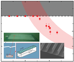
To qualitatively show the effects of nano-grass, trench dimensions and flow conditions (i.e. wall shear stress), the actual plastron lengths Lp on 60 mm long trenches were measured from all the images using ImageJ and plotted in figure 7, and the estimated theoretical plastron lengths Lss from (4.3) were drawn as colour-shaded ranges in the same figure for comparison, accordingly showing similar trends. If Lss < Lmax = 60 mm, the interface at the front of the 60 mm long trench should be depinned, and the plastron length could be observed as Lp = Lss. For the calculation of the theoretical estimation, the flow conditions of the experiments were used: air saturation level within s = 100 %–101 %, average water pressure as  ${\bar{P}_{water}}\sim 1500\;\textrm{Pa}$, and the wall shear stress on the SHPo surface τw estimated from the boat speeds U measured using the regression equation in Appendix D. Besides, the pressure fluctuation term, i.e. ${P^{\prime}_{water}}-{P^{\prime}_{air}}$, was intentionally ignored in the estimation range to allow the comparison. By increasing the boat speed beyond the ones used by Xu et al. (Reference Xu, Grabowski, Yu, Kerezyte, Lee, Pfeifer and Kim2020b), which did not observe any shear-driven wetting, we have observed severely degraded plastron on the same RE sample. In comparison, the NG and RE + NG samples were confirmed to have a clearly improved plastron stability and showed a better matching between the estimated ranges and experimental results. Although the theoretically estimated range of plastron length on RE was similar to those on NG and RE + NG, the metastable state of the re-entrant edge on RE was vulnerable to the many fluctuations in the environmental water and the pressure fluctuation of the highly turbulent flows under the boat.

Figure 7. Experimentally obtained plastron length Lp and theoretically estimated ranges of steady-state plastron length Lss as function of boat speed U for the experimental conditions in this study. (a) RE: trench with the re-entrant top edge and smooth surface, drawn blue. (b) NG: trench without the re-entrant top edge and nano-grass surface, drawn orange. (c) RE + NG: trench with re-entrant top edge and nano-grass surface, drawn red. The boat speed varied between ∼2 m s−1 < U < ∼7 m s−1. On each graph, the area above Lp = 60 mm was made dark to indicate an impossible range. Considering the numerous factors that were uncontrollable during the boat tests over several months, the experimental results match the theoretical estimations quite well.
The rear wetting made the plastron shorter than the estimation by (4.3) on NG and RE + NG especially for d = 90, 153 μm, but the effect was small (< ∼8 %). There was no significant difference between NG and RE + NG, as expected from the theory. It should be noted that, for simplicity, the theoretical wall shear stress on the SHPo surface τw was estimated from the wall shear stress on a smooth surface τw 0 by assuming 30 % drag reduction for all the speeds, which was the typical drag-reduction value from the previous works for p100 (Xu et al. Reference Xu, Grabowski, Yu, Kerezyte, Lee, Pfeifer and Kim2020b, Reference Xu, Yu, Kim and Kim2021) with gas fraction w/p = 0.9 in turbulent boundary flows for U > ∼5 m s−1. Although the theoretical wall shear stress should be 10–20 % larger than the estimated ones used in figure 7 for U < ∼5 m s−1, this effect was expected to be ignorable because a larger Lss would not change the fact that all the surfaces should have a pinned plastron (i.e. Lp = L < Lss) at low speeds (i.e. U < ∼5 m s−1) anyway due to the small wall shear stress. Besides, the theoretical shear stress for p75 should be 5 %–10 % larger than that on p100 in the same water flow due to the smaller pitch (Xu et al. Reference Xu, Yu, Kim and Kim2021), increasing Lss values for p75 surfaces by 5 %–10 %, while the experimental values will still fit the estimated values reasonably well. We note the theoretically estimated steady-state length Lss of (4.3) was for pinned plastron, while the experimentally measured Lp was for both pinned and slightly degraded plastron due to the finite resolution of observation. Unfortunately, the shear-driven drainage model in the current form (Wexler et al. Reference Wexler, Jacobi and Stone2015; Liu et al. Reference Liu, Wexler, Schönecker and Stone2016) does not allow us to quantitatively estimate how a slight degradation of plastron would affect its steady-state length. However, we believe the effect was minor because a slightly degraded plastron is unstable with a very short lifetime in the current experiment, making its population small in the measured data. Most importantly, NG and RE + NG have been demonstrated to maintain a pinned (including slightly degraded) plastron in the 60 mm long trench in turbulent boundary layer flows up to 7.2 m s−1 in accordance with the theoretical estimation, suggesting a direction toward high-performance SHPo surfaces for drag reduction.
5. Conclusion
To evaluate longitudinal micro-trench SHPo surfaces in high-speed flows of open water, which represent the operating conditions of common watercraft, we have studied how the sustainability of pinned plastron is affected by the pressure, air saturation level and wall shear of the water, and how the trends may be distorted by other factors, such as trench boundaries, surfactant and turbulent fluctuation. To model the effect of water pressure, an existing theory was used. To model the effect of wall shear stress of flowing water, another existing theory was used after a scale analysis revealed the diffusion of trapped air by the wall shear is small for the tested flow conditions. Distortions by the dynamic effect of flows were anticipated at the front and rear ends of the trench and corroborated by a numerical simulation. To evaluate the theoretical models and the distorting effects, micro-trench SHPo surfaces with combinatorial variations of trench width, trench depth, trench length and nano-roughness have been prepared and tested underneath a 13 foot motorboat in brackish water at a sea mouth. A unique observation technique using two underwater cameras was employed to differentiate pinned (and slightly degraded) plastrons from degraded (and no) plastrons rather than the common practice of determining whether the plastron is present or depleted. The experimental results corroborated the theoretical estimations reasonably well, considering the many assumptions in the models and the uncertainties inevitable in the field tests. When the trench surfaces were coated with nano-grass, nearly all the trenches tested were confirmed to have a pinned (or slightly degraded) plastron. This work contributed to designing SHPo surfaces geared toward field conditions for drag reductions, anti-biofouling, anti-corrosion, etc.
Supplementary movie
Supplementary movie is available at https://doi.org/10.1017/jfm.2023.184.
Acknowledgements
The authors thank H. Stone and P. Luzzatto-Fegiz for the discussions on the shear-driven drainage and the surfactant effect, respectively, and C.M. Carter for reviewing the manuscript.
Funding
This work was supported by NSF 1336966 and 2030404.
Declaration of interests
The authors report no conflict of interest.
Appendix A. Videos of plastron loss by shear drainage at high-speed flows
Underwater videos of the longitudinal trench SHPo surface used by Xu et al. (Reference Xu, Grabowski, Yu, Kerezyte, Lee, Pfeifer and Kim2020b) and tested at two different maximum speeds of boat are shown in Movie S1. The sample was filled with 7 cm long trenches made of re-entrant edges and smooth sidewalls (i.e. type RE by the designation of this report). For these close-up videos, two side cameras were used simultaneously (differently from the use of one side camera in the main study) to cover an entire sample. The top videos confirmed a pinned plastron being maintained at speeds up to 8 knots (4.1 m s−1), which was near the maximum boat speed tested by Xu et al. (Reference Xu, Grabowski, Yu, Kerezyte, Lee, Pfeifer and Kim2020b), and the bottom videos showed the plastron being drained out by the shear stress at 10 knots (5.1 m s−1) and completely lost at 13 knots (6.7 m s−1), motivating the current study of developing the nano-grass-covered SHPo surfaces. Following the test procedures by Xu et al. (Reference Xu, Grabowski, Yu, Kerezyte, Lee, Pfeifer and Kim2020b) and unlike the current report, the air saturation level was not measured for this visualization.
Appendix B. Scaling comparison of the three air fluxes in a trench
The air diffusion across the air–water interface (meniscus) will lead to a diffusion-driven air flow inside the plastron. Since air diffusion rate across the meniscus varies with the Laplace pressure and meniscus area, the diffusion-driven flow flux scales as  ${q_d}\sim {k_p}\sigma L$, where kp is the interfacial mass transfer coefficient, σ is the air–water interfacial tension and L is the trench length. In turbulent boundary layer flows, kp is defined by ‘film theory’ (Cussler & Cussler Reference Cussler and Cussler2009) as
 \begin{equation}{k_p} = \frac{{{D_{air}}}}{{{\delta _c}}}\frac{M}{{{k_H}{\rho _{air}}}},\end{equation}
where Dair is the diffusion coefficient of air (i.e. 1.75–2.00 × 10⁻⁵ cm2 s−1); M is the molecular weight of air (i.e. 29 g mol−1); ρair is the density of air (i.e. 0.0012 g cm−3); δc is diffusion length, which depends on the flow condition. Henry's constant kH (i.e. 1.21–1.34 atm mM−1) is irrelevant to the hydrostatic pressure unless the immersion depth is very large (e.g. kH increases ∼14 % at immersion depth ∼1000 m Enns, Scholander & Bradstreet Reference Enns, Scholander and Bradstreet1965). Ling et al. (Reference Ling, Katz, Fu and Hultmark2017) studied the effect of Reynolds number on diffusion length in turbulent boundary layer flow over a SHPo surface and found the relation between the Sherwood number  $S{H_{\varTheta 0}}$ and friction Reynolds number Reτ 0, where subscript 0 indicates a smooth surface, as $S{H_{\varTheta 0}} = 0.34Re_{\tau 0}^{0.913}$. Here, $SH_{\varTheta {0}}=\varTheta_{0}/\delta_{c}$, where $\varTheta_{0}$ is the momentum boundary layer thickness on a smooth surface and approximated to be ${\varTheta_0}/\hat{x} = 0.01277Re_x^{ - 0.1341}$ (Nagib, Chauhan & Monkewitz Reference Nagib, Chauhan and Monkewitz2007) for the purpose of scaling estimation, with the Reynolds number defined as Rex = U $\hat{x}$/ν, where $\hat{x}$ is the streamwise distance from the leading edge of immersed boat hull to the sample surface ( $\hat{x}$ is labelled as ∼2 m in figure 5a). Since the boat is tilted and elevated (by planing) when it speeds up, i.e. $\hat{x}$ decreases slightly with U, the tilting angle and waterline of the boat were measured for all the individual experiments to estimate $\hat{x}$ for each test run. For the purpose of estimating friction Reynolds number $R{e_{\tau 0\; }} = {\delta _0}{({\tau _{w0}}/\rho )^{0.5}}/\nu$, the boundary layer thickness on the smooth surface δ 0 can be approximated to be ${\delta _0}/\hat{x} = 0.16Re_x^{ - 1/7}$ (White & Majdalani Reference White and Majdalani2006) for the purpose of scaling estimation, and the shear stresses on smooth surface τw 0 were established in Appendix D. In the turbulent boundary layer flow under the boat set-up, using the relations above, we can estimate δc at the minimum and maximum Reynolds numbers ( $R{e_x} = 5.17 \times {10^6}$ and 1.10 × 10⁷, corresponding to the minimum and maximum boat speed U = 2.0 m s−1 and 7.2 m s−1) to be 6.75 and 1.93 μm, respectively. The parameters estimated using the relations above are listed in table 2. By inputting these values in (B1), we obtain ${k_p} = 0.5 \times {10^{ - 10}}{-}1.6 \times {10^{ - 10}}\;\textrm{m}\;{\textrm{(s}\ \textrm{Pa)}^{ - 1}}$.
Table 2. Approximation for parameters on boat tests. Here, U and x were measured from experiments, and other parameters were estimated from theoretical equations.

By considering micro-trenches with aspect ratio d/w = 1 and gas fraction w/p = 0.9, based on (2.6) and (2.7), the shear-driven flow and the pressure-driven flow scale as  ${q_{sl}}\sim {10^{ - 3}}\tau {w^3}\mu _{air}^{ - 1}$ and ${q_p}\sim {10^{ - 2}}{h^3}\sigma \mu _{air}^{ - 1}{L^{ - 1}}$, respectively. Then, we can estimate the magnitude of each flux inside the trench by substituting the exemplary values into the scaling equations. By assuming (i) the trench has width and depth of w = h = 90 μm and length of L = 60 mm and (ii) the shear stress on the SHPo surface is τw ∼ 50 Pa, the scaling equations lead to ${q_d}/{q_{sl}}\sim O({10^{ - 4}})$ and ${q_d}/{q_p}\sim O({10^{ - 4}})$. Therefore, we conclude that, for the trench geometries and flow conditions relevant to the current study, the diffusion-driven flow is negligibly small compared with the shear-driven flow and pressure-driven flow.
Appendix C. Numerical simulation for water pressure on and air pressure in a trench
To check the quantitative relevance of the deviations of water pressure Pwater and air pressure Pair anticipated in figure 2(d), a numerical simulation of a two-phase turbulent boundary layer flow was performed on the three-dimensional modelled domain using the unsteady Reynolds-averaged Navier–Stokes (RANS) technique and volume of fluid (VOF) multiphase model provided by ANSYS Fluent 17.1 (Ansys Inc, PA, USA). The geometric configuration of the numerical simulation is shown in figure 8(a) with the boundary conditions. Here, the notation is such that  $\hat{x}$, $\hat{y}$ and $\hat{z}$ denote the streamwise, wall-normal and spanwise coordinates, and corresponding time-averaged velocity components are u, v and w. To trigger a bypass transition from a laminar to turbulent flow, a rectangular rod is introduced near the inlet. The computational domain sizes in the streamwise, wall-normal and spanwise directions were 0.1202 m, 0.02 m and $7.5 \times {10^{ - 5}}\;\textrm{m}$, respectively, with corresponding grid numbers of 2404, 151 and 30. For a trench that is positioned at $\hat{x}$ = 0.0602 m away from the inlet, the sizes in the streamwise, wall-normal and spanwise directions were 0.01 m, $5.06 \times {10^{ - 5}}\;\textrm{m}$ and $6.75 \times {10^{ - 5}}\;\textrm{m}$, respectively, with corresponding grid numbers of 200, 41 and 27. The governing equations for the unsteady RANS simulations including VOF model were discretized through the finite volume method with second-order central difference scheme and fully implicit second-order temporal discretization, and a pressure-based solver was adopted for an incompressible flow with the k–ω shear-stress transport turbulence model (Menter Reference Menter1994).

Figure 8. Three-dimensional simulation for a turbulent flow of water over a micro-trench filled with air, assuming a flat air–water interface. (a) Schematic of the computational domain and boundary conditions. (b) Velocity vector superimposed with the volume fraction contour (the axes are not scaled). The blue and red contours on the  $\hat{x}\hat{y}$-plane indicate the water and the air phases, respectively. (c) Mean pressure and (d) root mean square of the turbulent pressure fluctuations for the water and air right above and below the interface $(\hat{y} = {\hat{y}_{interface}} \pm 1.0 \times {10^{ - 6}}\;\textrm{m)}$, respectively, or at the wall ( $\hat{y}$ = 0). The water and air pressure variations along the trench corroborate figure 2(d).
Assuming U = 2 m s−1 and Patm = 101.3 kPa, figure 8(b) shows the time-averaged velocity vector superimposed with the void fraction contour α on the  $\hat{x}\hat{y}$-plane that are extracted in the middle of the trench $(\hat{z} = 3.75 \times {10^{ - 5}}\;\textrm{m)}$. The air–water interface stays almost flat along the trench. Over the trench, a slip of the water flow (here, the spatially averaged slip velocity is estimated to be 1.37 m s−1) is clearly observed, and the backflow is generated in the air within the trench by the slip of the interface. Finally, figure 8(c) shows the mean water and air pressure right above and below the interface, respectively. The decrease and increase of the mean water pressure near the front and rear ends of the trench, respectively, and the linear increase of the mean air pressure along the trench confirm the trend anticipated in figure 2(d). The decrease of the mean water pressure at the front end is caused by the flow acceleration as water flows from the no-slip surface to the slip interface. On the other hand, the increase of the mean water pressure at the rear end is caused by the flow deceleration as water flows from the slip interface to the no-slip surface. The increase of the mean air pressure along the trench is caused by the flow impingement on the rear wall. In figure 8(d), small turbulent pressure fluctuations are observed in the water on the interface, whereas no turbulent pressure fluctuation is observed in the air underneath the interface.
Appendix D. Experiments for shear stress vs. boat speed
The shears stress on a smooth surface τw 0 underneath the boat has been measured with the custom shear sensor (Xu et al. Reference Xu, Arihara, Tong, Yu, Ujiie and Kim2020a) over the range of boat speeds U used in the current study and plotted in figure 9. The power regression line, which fits the experimental data reasonably well (especially considering the varying environmental conditions the field tests are subjected to), is used to estimate the wall shear stress for the plastron observation runs. The power regression also ensures the shear stress is zero when the boat speed is zero. The shear stress on the SHPo surface, τw, is estimated as 0.7τw 0, which assumes 30 % drag reduction. The estimation for 30 % drag reduction of SHPo surface was confirmed by previous work on the same boat (Xu et al. Reference Xu, Grabowski, Yu, Kerezyte, Lee, Pfeifer and Kim2020b) and in a high-speed towing tank under similar flow condition (Xu et al. Reference Xu, Yu, Kim and Kim2021). The ∼30 % drag reduction has also been proven to be consistent by the authors’ recent experiments (unpublished), which used the same flow conditions as this study.

Figure 9. Wall shear stress on a smooth surface τw 0 at different boat speeds. The experimental data fit the power regression line.
Appendix E. Picture pairs of all the 12 samples taken underwater at 4 selected boat speeds

Figure 10. Sample images at speeds in the range 3.3–3.8 m s−1. Blue indicates a pinned or slightly depinned interface (i.e. h/w ≤ 0.17); yellow indicates a depinned interface (i.e. 0.17 < h/w < d/w); and red indicates no interface (i.e. h/w = d/w).

Figure 11. Sample images at speeds in the range 4.4–5 m s−1. Blue indicates a pinned or slightly depinned interface (i.e. h/w ≤ 0.17); yellow indicates a depinned interface (i.e. 0.17 < h/w < d/w); and red indicates no interface (i.e. h/w = d/w).

Figure 12. Sample images at speeds in the range 5.2–5.7 m s−1. Blue indicates a pinned or slightly depinned interface (i.e. h/w ≤ 0.17); yellow indicates a depinned interface (i.e. 0.17 < h/w < d/w); and red indicates no interface (i.e. h/w = d/w).

Figure 13. Sample images at speeds in the range 6.3–6.7 m s−1. Blue indicates a pinned or slightly depinned interface (i.e. h/w ≤ 0.17); yellow indicates a depinned interface (i.e. 0.17 < h/w < d/w); and red indicates no interface (i.e. h/w = d/w).
Appendix F. Experimental data
The experimental data is shown in table 3. Due to the limitations in the field experiments and as commonly done in the literature (Fukagata et al. Reference Fukagata, Kasagi and Koumoutsakos2006; Busse & Sandham Reference Busse and Sandham2012; Ling et al. Reference Ling, Katz, Fu and Hultmark2017), we used the estimated parameters based on flow conditions of smooth surface. The wall shear stress τw 0, at different boat speeds of different tests based on figure 9, was used for the calculation of the wall friction velocity  ${u_{\tau 0}} = {({\tau _{w0}}/\rho )^{1/2}}$. The non-dimensionalized length scale quantities were normalized using wall unit ${\delta _{v0}} = \nu {({\tau _{w0}}/\rho )^{ - 1/2}}$; for example, ${w^{ + 0}} = w/{\delta _{v0}}$. The wetting length of the boat, which is the distance between the sample and the leading end of the immersed hull, $\hat{x}$, was estimated based on the boat tilting angle and immersion depth.
Table 3. Experimental parameters. The Reynolds number based on boundary layer thickness is  $R{e_{\delta 0}} = U{\delta _0}/\nu$. The Weber number is defined as $W{e_{\tau 0}} = {\mu _{water}}{u_{\tau 0}}/\sigma$. The friction Reynolds number is $R{e_{\tau 0}} = {u_{\tau 0}}{\delta _{v0}}/\nu$. The trench length ${L^{ + 0}}$ is based on the longest trenches. The range of $L_{ss}^{ + 0}$ is determined from the range of air saturation measured during the experiments (i.e. 100%-101% in this study). For the plastron length, $L_p^{ + 0} = L_{ss}^{ + 0}$ if $L_{ss}^{ + 0} < {L^{ + 0}}$, and $L_p^{ + 0} = {L^{ + 0}}$ if $L_{ss}^{ + 0} > {L^{ + 0}}$.


 Open access