


1. Introduction
Liquid fuels are much used in combustion-based transport and industry applications because of their availability, high energy density and easy storage in atmospheric conditions (Sharma & Ghoshal Reference Sharma and Ghoshal2015). The direct injection of liquid fuels as spray in a combustion chamber is the preferred option in state-of-the-art designs, mostly because of its high efficiency and simplicity. In that context, the vaporization of the liquid fuel is a key stage before the chemical energy stored in the fuel is released through combustion.
Due to its technological importance, the understanding of the vaporization of fuel droplets has been of great attention. Forced by the lack of computational power, the first theoretical models were based on order-of-magnitude analyses in which the properties of the fluids were assumed to be constant, both phases were in quasi-steady state and radiation was neglected (Spalding Reference Spalding1959; Crespo & Liñán Reference Crespo and Liñán1975; Law Reference Law1982; Kuo Reference Kuo1986; Abramzon & Sirignano Reference Abramzon and Sirignano1989; Liñán & Williams Reference Liñán and Williams1993).
Recent improvements in calculation capabilities have motivated the formulation of new models that make use of more sophisticated physics to consider the unsteady evaporation of mono- and multicomponent droplets with variable fluid properties (Yang & Wong Reference Yang and Wong2001; Sazhin Reference Sazhin2006; Azimi et al. Reference Azimi, Arabkhalaj, Ghassemi and Markadeh2017; Lupo & Duwig Reference Lupo and Duwig2018; Fang et al. Reference Fang, Chen, Li and Wang2019; Pinheiro et al. Reference Pinheiro, Vedovoto, da Silveira Neto and van Wachem2019; Ray, Raghavan & Gogos Reference Ray, Raghavan and Gogos2019). In spite of such improvements, often numerical predictions do not match with experiments and it is common to utilize correlations or semi-empirical parameters to improve the agreement with measurements (Maqua, Castanet & Lemoine Reference Maqua, Castanet and Lemoine2008), a practice that hinders the understanding of the underlying physics controlling the vaporization of liquid fuels. Leaving aside the work by Yang & Wong (Reference Yang and Wong2001), Lage & Rangel (Reference Lage and Rangel1993) and Tseng & Viskanta (Reference Tseng and Viskanta2005, Reference Tseng and Viskanta2006), the effect of radiation is not included in the models for the evaporation of single droplets.
Experimental studies under different conditions have been used to study mono- and multicomponent droplets including suspended droplets from fibers (Nomura et al. Reference Nomura, Ujiie, Rath, Sato and Kono1996; Ghassemi, Baek & Khan Reference Ghassemi, Baek and Khan2006; Chauveau et al. Reference Chauveau, Halter, Lalonde and Gökalp2008; Hallett & Beauchamp-Kiss Reference Hallett and Beauchamp-Kiss2010; Erbil Reference Erbil2012; Han et al. Reference Han, Zhao, Fu, Zhang, Pang and Li2015), levitating droplets (Gregson et al. Reference Gregson, Ordoubadi, Miles, Haddrell, Barona, Lewis, Church, Vehring and Reid2019; Niimura & Hasegawa Reference Niimura and Hasegawa2019; Sasaki et al. Reference Sasaki, Hasegawa, Kaneko and Abe2020), free falling droplets (Lee & Law Reference Lee and Law1992; Sirignano Reference Sirignano2010; Hillenbrand & Brüggemann Reference Hillenbrand and Brüggemann2020; Muelas et al. Reference Muelas, Carpio, Ballester, Sánchez and Williams2020), sessile droplets on heated and not-heated surfaces (Cazabat & Guena Reference Cazabat and Guena2010; Erbil Reference Erbil2012) and droplets evaporating in heated air flows with elevated temperatures and pressures (Sirignano Reference Sirignano2010). Various experimental techniques, each with advantages and disadvantages, have been instrumental in understanding complex phenomena such as puffing (Avulapati et al. Reference Avulapati, Ganippa, Xia and Megaritis2016; Shinjo et al. Reference Shinjo, Xia, Ganippa and Megaritis2016), particle deposition (Shmuylovich, Shen & Stone Reference Shmuylovich, Shen and Stone2002; Sefiane, Tadrist & Douglas Reference Sefiane, Tadrist and Douglas2003), Marangoni currents (Gurrala et al. Reference Gurrala, Katre, Balusamy, Banerjee and Sahu2019; Gao et al. Reference Gao, Zhang, Kong and Zhang2020) or the importance of surface hydrophobicity and wettability for the evaporation of drops and droplets (He, Liao & Qiu Reference He, Liao and Qiu2017).
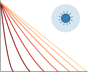
As part of a wider effort devoted to increase the basic understanding of droplet evaporation, in this paper we are concerned with the analysis of the vaporization in microgravity conditions of an individual droplet of radius  $a(t)$ in a stagnant, hot and inert nitrogen environment at a temperature $T_{\infty }$ and a pressure $p_{\infty }$. Pure nitrogen atmospheres are typically employed in droplet vaporization experimental set-ups, and then in numerical simulations, to avoid chemical reactions that could lead to uncontrolled variations in the temperature and concentration fields or even produce autoignition during droplet vaporization. This possibility, very real even for low ambient temperature, has been considered elsewhere (Millán-Merino Reference Millán-Merino2020; Millán-Merino et al. Reference Millán-Merino, Fernández-Tarrazo, Sánchez-Sanz and Williams2020). This simple configuration is especially suited for testing and improving the fundamental understanding of droplet vaporization. Our purpose is to use only first principles to carry out our analysis, avoiding the introduction of semi-empirical parameters or correlations intended to improve the match between numerical results and experimental measurements.
To solve the problem sketched in figure 1 we use the formulation, physical model and numerical method introduced in Millán-Merino (Reference Millán-Merino2020). This method is validated below by comparing our numerical results with experimental measurements and previous simulations of single-component  $n$-heptane and ethanol droplets and multicomponent ethanol–water and $n$-dodecane– $n$-hexadecane droplets. In the latter, the large difference in the boiling temperatures of both components and the non-ideal vaporization properties of the liquid phase introduce complexities in the analysis that greatly modify the features of the evaporation process.

Figure 1. Sketch of the spherically symmetric set-up.
In the following sections, we consider the vaporization of both monocomponent and multicomponent droplets, dedicating special attention to ethanol–water droplets because of the technological relevance as a cleaner alternative to petrol-based fuels.
The paper is organized as follows. In § 2 we include the whole formulation in detail, including the conservation equations, boundary and initial conditions and constitutive relations for the physical properties of both the liquid and gas phases. Those readers familiar with the equations can skip this section in a first reading of the paper without losing track of the main results. In § 3 we carry out an order-of-magnitude analysis to gain insight into the physically relevant phenomena and define the relevant time scales of the problem. In § 4 we focus our efforts on the analysis of monocomponent single-droplet vaporization using the scales identified in § 3. In § 5 we shift our attention to the relevant case of multicomponent droplet vaporization before presenting the main conclusions in § 6.
2. Formulation
We consider here the case of a single droplet with initial radius of  $a_0$ in an infinite stagnant atmosphere without gravity or forced flow as sketched in figure 1. In these conditions, the flow has spherical symmetry provided that the initial conditions satisfy this property. As we justify in § 3, the gas phase can be considered in quasi-steady state. On the contrary, an accurate description of the vaporization problem requires a fully transient formulation for the liquid phase. The spherically symmetric problem of droplet evaporation in microgravity conditions is mathematically described by the mass, species and energy conservation equations for the liquid phase,
 \begin{gather} \frac{\partial \rho_{\ell}}{\partial t} + \frac{1}{r^{2}} \frac{\partial}{\partial r}(r^{2}\rho_{\ell} u_{\ell} ) = 0, \end{gather}
 \begin{gather}\frac{\partial (\rho_{\ell} Y_{{\ell},i}) } {\partial t} + \frac{1}{r^{2}}\frac{\partial}{\partial r} (r^{2}\rho_{\ell} Y_{{\ell},i} u_{\ell}) = -\frac{1}{r^{2}}\frac{\partial}{\partial r} (r^{2} J_{{\ell},i}),\quad i=1,\ldots,N_{\ell}\,|\,i\neq I, \end{gather}
 \begin{gather}\frac{\partial (\rho_{\ell} h_{\ell})}{\partial t} + \frac{1}{r^{2}}\frac{\partial}{\partial r} ( r^{2}\rho_{\ell} h_{\ell} u_{\ell} ) = - \frac{1}{r^{2}} \frac{\partial}{\partial r} (r^{2} q_{\ell}), \end{gather}
and for the gas phase,
 \begin{gather} \frac{\mathrm{d}}{\mathrm{d} r}(r^{2}\rho_{{g}} u_{{g}} ) = 0, \end{gather}
 \begin{gather}\frac{\mathrm{d}}{\mathrm{d} r} (r^{2}\rho_{{g}} Y_{{{g}},i} u_{{g}}) = -\frac{\mathrm{d}}{\mathrm{d} r} (r^{2} J_{{{g}},i}),\quad i=1,\ldots,N_{{g}}\,|\,i\neq I, \end{gather}
 \begin{gather}\frac{\mathrm{d}}{\mathrm{d} r} (r^{2}\rho_{{g}} h_{{g}} u_{{g}}) = -\frac{\mathrm{d}}{\mathrm{d} r} (r^{2} q_{{g}}), \end{gather}
with  $\rho _{\beta }$, $u_{\beta }$, $Y_{\beta ,i}$ and $h_{\beta }$ being the density, the velocity, the mass fraction and the thermal enthalpy of the mixture, respectively. The subscript $i$ represents the $i$th species in both the liquid phase $\beta =\ell$ inside the droplet and the gas phase $\beta ={g}$, and $i=I$ denotes the most abundant species in each phase. Liquid-phase density $\rho _{\ell }$ may change due to local temperature and/or composition changes which, according to continuity equation (2.1), implies changes in the velocity field $u_{\ell }$.
The species mass flux term for the gas phase in (2.5) is calculated with the mixture-averaged model (Kee, Warnatz & Miller Reference Kee, Warnatz and Miller1983) with conservative flux correction (Coffee & Heimerl Reference Coffee and Heimerl1981):
 \begin{equation} J_{{{g}},i} = -\rho_{{g}} Y_{{g},i} \left( V_{d, i}^{0} + V_{d}^{c} \right), \end{equation}
where  $V_{d, i}^{0} = - (D_{{g},i}/X_{{g},i}) (\partial X_{{g},i}/\partial r)$ and $V_{d}^{c} = - \sum _{i=1}^{N_{{g}}} Y_{{g},i} V_{d, i}^{0}$, in which $X_{\beta ,i}=Y_{\beta ,i}W/W_i$ is the mole fraction, with $W$ and $W_{i}$ being the average and $i$th species molar mass, respectively, and $D_{{g},i} = (1-Y_{{g},i}) /({\sum _{{j{\neq}i}}^{N_{{g}}} {X_{{g},j}/D_{{g},ji}}}$) is the mixture diffusion coefficient, with $D_{{g},ij}$ the binary diffusion coefficient, for the pair of species $i$ and $j$, obtained from the kinetic theory (Hirschfelder, Curtiss & Bird Reference Hirschfelder, Curtiss and Bird1964). For the liquid phase, (2.2), the diffusive mass flux term is calculated using Fick's law:
 \begin{equation} J_{\ell,i} = -\rho_{\ell}D_{\ell,i} \frac{\partial Y_{\ell,i} }{\partial r} \end{equation}
and the mixture diffusion coefficient is determined using the Wilke–Chang equation (Wilke & Chang Reference Wilke and Chang1955):
 \begin{equation} D_{\ell,i} = 1.173 \times 10^{-16} \frac{\sqrt{\displaystyle\sum_{j{\neq}i}^{N_\ell}X_{\ell,j}\varphi_j W_{j}} T } {\mu_{\ell} {V}_{\ell,i}^{0.6}}, \end{equation}
where  $\mu _{\ell }$ is the mixture viscosity and ${V}_{\ell ,i}$ the molar volume. The association factor takes the values $\varphi _i=2.6$ for water, $\varphi _i=1.5$ for ethanol and $\varphi _i=1$ otherwise. In the energy equations (2.3) and (2.6), the thermal heat flux term $q_{\beta }$ is obtained from generalized Fourier's law:
 \begin{equation} q_{\beta} = -k_{\beta}\frac{\partial T}{\partial r} + \sum_{i=1}^{N_{\beta}} J_{\beta,i}h_{\beta,i}, \end{equation}
where  $k_{\beta }$ is the thermal conductivity of the $\beta$ phase and $N_{\beta }$ denotes the number of species in each phase. Soluble species exist in both phases ( $i=1,\ldots , N_{\ell }$) but non-soluble species only exist in the gas phase ( $i=N_{\ell }+1,\ldots , N_{{g}}$). Only the solubilities of liquid ethanol and water have been considered. The most abundant species in each phase $(i=I)$ is obtained as $Y_{{\beta },I} = 1 - \sum _{i{\neq}I}^{N_{\beta }}Y_{{\beta },i}$.
Equations (2.1)–(2.10) are supplemented with the equations of state of the gas written in the quasi-isobaric approximation  $p_\infty /\rho _{{g}}=T R_{{g}}$, with $R_{{g}} = \mathcal {R}/W$ and $1/W = \sum _{1}^{N_{{g}}} Y_i/W_i$. Notice that this approximation makes it unnecessary to solve the momentum equation unless the pressure differences, ${\rm \Delta} p = p - p_\infty$, are sought (Williams Reference Williams2018). The density of the mixture in the liquid phase is computed as in Aalto et al. (Reference Aalto, Keskinen, Aittamaa and Liukkonen1996) using the expression $\rho _{\ell }=( \sum ^{N_{\ell }}_{i=1} X_{\ell ,i} {\rho _{\ell ,i}^{1/2}} )^{2}$, in which the individual densities of liquid species are obtained by fitting published experimental data (Banipal, Garg & Ahluwalia Reference Banipal, Garg and Ahluwalia1991; Khasanshin, Shchamialiou & Poddubskij Reference Khasanshin, Shchamialiou and Poddubskij2003; Caudwell et al. Reference Caudwell, Trusler, Vesovic and Wakeham2004; Kadlec, Henke & Bubnik Reference Kadlec, Henke and Bubnik2010; Outcalt, Laesecke & Fortin Reference Outcalt, Laesecke and Fortin2010; Engineering ToolBox 2013; Michailidou et al. Reference Michailidou, Assael, Huber, Abdulagatov and Perkins2014) using the expression introduced by Svehla (Reference Svehla1995):
 \begin{equation} \log{ \rho_{\ell,i} } = A_{\rho,i} \log(T) + \frac{B_{\rho,i}}{T} + \frac{C_{\rho,i}}{T^{2}} + D_{\rho,i} + E_{\rho,i} T + F_{\rho,i} T^{2} . \end{equation}
2.1. Constitutive relations
Both liquid and gas phases are considered ideal mixtures with heat capacity and enthalpy calculated as  $c_{p_{\beta }}=\sum ^{N_{\beta }} Y_{\beta ,i}c_{p_{\beta ,i}}$ and $h_{\beta }=\sum ^{N_{\beta }} Y_{\beta ,i}h_{\beta ,i}$, in terms of the heat capacity $c_{p_{\beta ,i}}$ and thermal enthalpy $h_{\beta ,i}$ of species $i$ in phase $\beta$.
The thermodynamic properties  $c_{p_{\beta ,i}}$ and $h_{\beta ,i}$ of pure species are obtained using the NASA polynomials (McBride Reference McBride1993), where the coefficients are obtained whenever possible from the San Diego mechanism database (UCSD 2016). Data for those species not available in the San Diego database were taken from Burcat's database (Goos, Burcat & Ruscic Reference Goos, Burcat and Ruscic2010).
The gas-phase molecular transport coefficients  $D_{{g},ij}$ and $k_{{g},i}$ are obtained using the expression derived directly from the kinetic theory (Hirschfelder et al. Reference Hirschfelder, Curtiss and Bird1964) using the transport database of the San Diego mechanism (UCSD 2016), while $k_{{g}}$ is obtained using the standard mixture average formula (Mathur, Tondon & Saxena Reference Mathur, Tondon and Saxena1967):
 \begin{equation} k_{{g}} = \frac{1}{2}\left( \sum_{i=1}^{N_{g}}X_{{g},i}k_{{g},i} + \frac{1}{\displaystyle\sum_{i=1}^{N_{g}}X_{{g},i}/k_{{g},i}}\right). \end{equation}
For the liquid phase, the mixture thermal conductivity  $k_{\ell }$ was obtained from a generalization of Filippov's equation (Filippov Reference Filippov1955):
 \begin{equation} k_\ell = \sum_{i=1}^{N_\ell} Y_{\ell,i} \left( k_{\ell,i} - \sum_{j=i+1}^{N_\ell}K_{i,j}Y_{\ell,j}\left| k_{\ell,i}-k_{\ell,j} \right| \right), \end{equation}
where Filippov's constant is  $K_{i,j}=0.72$. The conductivity of the pure species is computed using the correlation (Svehla Reference Svehla1995)
 \begin{equation} \log { k_{\ell,i} } = A_{k,i} \log(T) + \frac{B_{k,i}}{T} + \frac{C_{k,i}}{T^{2}} + D_{k,i} + E_{k,i} T + F_{k,i} T^{2}, \end{equation}
in which the coefficients are obtained by fitting with the experimental data published in Kadlec et al. (Reference Kadlec, Henke and Bubnik2010), Engineering ToolBox (2013), Assael et al. (Reference Assael, Charitidou, de Castro and Wakeham1987), Burgdorf et al. (Reference Burgdorf, Zocholl, Arlt and Knapp1999), Tanaka et al. (Reference Tanaka, Itani, Kubota and Makita1988) and Dortmund Data Bank (2019). The viscosity of the liquid mixture is evaluated using the Grunberg and Nissan equation: (Grunberg & Nissan Reference Grunberg and Nissan1949)
 \begin{equation} \mu_{\ell}=\exp\left( \sum_{i=1}^{N_\ell}X_{\ell,i} \ln\mu_{\ell,i} \right), \end{equation}
where the viscosity of the pure species is obtained using an expression analogous to (2.14) for the experimental results of Kadlec et al. (Reference Kadlec, Henke and Bubnik2010), Engineering ToolBox (2013), Sagdeev et al. (Reference Sagdeev, Fomina, Mukhamedzyanov and Abdulagatov2013), Michailidou et al. (Reference Michailidou, Assael, Huber, Abdulagatov and Perkins2014), Caudwell et al. (Reference Caudwell, Trusler, Vesovic and Wakeham2004), Koller et al. (Reference Koller, Klein, Giraudet, Chen, Kalantar, van der Laan, Rausch and Froba2017) and Wohlfarth (Reference Wohlfarth2008). Even though the momentum equation is not integrated and no viscous terms are included in the formulation, the liquid-phase viscosity is required in (2.9) to obtain the effective diffusivity of the species in the liquid phase. The numerical values of the coefficients  $A, B, C, D, E$ and $F$ for density, conductivity and viscosity of the liquid-phase species are given in the Appendix.
2.2. Boundary conditions
Boundary conditions are required at the centre of the droplet and in the far field:
 \begin{gather} r=0: \quad \frac{\partial T_{\ell}}{\partial r}=\frac{\partial Y_{\ell,i}}{\partial r}=u_{\ell}=0, \end{gather}
 \begin{gather}r \rightarrow \infty: \quad T_{{g}}-T_{\infty}= Y_{{g},i}-Y_{\infty,i}=0, \end{gather}
while the boundary conditions at the liquid–gas interface are obtained by imposing the continuity of the temperature field and the conservation of species mass and energy in a control volume extending from  $r = a(t) - \delta$ to $r = a(t) + \delta$ in the limit $\delta \rightarrow 0$, yielding
 \begin{align} -{\dot m}''(Y_{{g},i}-Y_{\ell,i})_{r=a}&=-(J_{{g},i}-J_{\ell,i})_{r=a},\quad i=2,\ldots,N_{\ell}, \end{align}
 \begin{align} -{\dot m}''(Y_{{g},i})_{r=a} &=-(J_{{g},i})_{r=a},\quad i=N_{\ell}+2,\ldots,N_{{g}}, \end{align}
 \begin{align} \left( T_{\ell} \right)_{r=a} &= \left( T_{{g}} \right)_{r=a} = T_s, \end{align}
 \begin{align} -\dot m'' \sum_{i=1}^{N_l} \left( Y_{\ell,i} {L}_i(T_s) \right)_{r=a} &= \left( k_{{g}} \frac{\partial T}{\partial r} - k_{\ell} \frac{\partial T}{\partial r} \right)_{r=a} \nonumber\\ &\quad +\alpha_{{eff}}\sigma\left(T_\infty^{4}-T_s^{4}\right) - \sum_{i=1}^{N_l} \left( J_{\ell,i} {L}_{i}(T_s) \right)_{r=a}, \end{align}
where  $a(t)$ is the instantaneous time-dependent radius of the droplet at a generic time $t$, determined by the surface mass balance
 \begin{equation} {{ -{\dot m}''=\rho_{\ell}(u_{\ell}-{\dot a})_{r=a}=\rho_{{g}}(u_{{g}}-{\dot a})_{r=a}, }}\end{equation}
where  ${{-\dot m''}}$ is the mass vaporization rate per unit of surface area, $T_s$ is the droplet surface temperature and ${\dot a}={\textrm {d}}a/{\textrm {d}}t$. The vaporization heat of each species is calculated as ${L}_i(T_s) = h_{{g},i}(T_s)-h_{\ell ,i}(T_s) + {L}_{i}^{{ref}}$, with ${L}_i^{{ref}}$ representing the vaporization heat at the reference temperature. Notice that an optically thin radiation model is included in our model through (2.21), where $\sigma$ is the Stefan–Boltzmann constant and $\alpha _{{eff}}=0.93$ is the effective absorption coefficient as found by Yang & Wong (Reference Yang and Wong2001) and Tseng & Viskanta (Reference Tseng and Viskanta2005).
Additionally, imposing the conservation of the chemical potential at the interface we obtain the Clausius equation (Criado-Sancho & Casas-Vázquez Reference Criado-Sancho and Casas-Vázquez1997):
 \begin{equation} (Y_{{g},i})_{r=a}=\left(Y_{\ell,i}\frac{W_{\ell}}{W_{{g}}}\right)_{r=a} \frac{p_{{atm}}}{{{p(r=a)}}} \gamma_i \exp \left( { \int_{T_{{b},i}}^{T_s}\frac{{L}_i(T)}{R_{{g},i}T^{2}}\mathrm{d}T } \right),\quad i=1,\ldots, N_{\ell}, \end{equation}
where  $T_{{b},i}$ is the boiling temperature at atmospheric pressure ( $p_{{atm}}=101\,325$ Pa) and $R_{{g},i} = \mathcal {R}/W_i$ and $\gamma _i$ are, respectively, the specific gas constant and the activity coefficient for species $i$, obtained using the UNIFAC method (Fredenslund, Gmehling & Rasmussen Reference Fredenslund, Gmehling and Rasmussen1977). The pressure of the fluid at the droplet surface is equal to the ambient pressure $p(r=a)=p_\infty =101\,325$ Pa in the low-Mach-number approximation used in the paper.
2.3. Initial conditions
We consider here the simplest case of a droplet with uniform composition and temperature that is placed at  $t=0$ in an infinitely large homogeneous gaseous ambient. We assume that at $t=0$ the droplet, of uniform temperature and composition, is suddenly placed unperturbed in the gaseous ambient:
 \begin{equation} t=0: u_\ell = Y_{\ell,i} - Y_{\ell,i,0} = T_{\ell} - T_{d_0} =0;\quad i=1,\ldots, N_{\ell}, \end{equation}
Notice that, because of the quasi-steady assumption for the gas phase, it is not necessary to smooth the initial condition in the gas phase near the droplet interface, as was done in a previous work (Millán-Merino et al. Reference Millán-Merino, Fernández-Tarrazo, Sánchez-Sanz and Williams2020) to avoid numerical instabilities. The comparison between both approaches in this work provides further validation for the approximation used there.
2.4. Numerical method
The set of equations (2.1)–(2.6) together with the boundary conditions (2.16)–(2.21) and initial conditions (2.24) are discretized in a spherical domain using a second-order, finite-volume discretization for the spatial derivatives and a first-order backward Euler discretization for the temporal derivatives. The resulting set of equations is solved using a modified Newton–Raphson method that minimizes an error function  $f$ formed subtracting the left- and right-hand-side terms of the equations. A non-uniform grid with typically 80 points is used to discretize a fluid domain that spans $100 a_0$, with a maximum clustering of points at the gas–liquid interface where the maximum gradients are located. The minimum and maximum grid steps are ${\rm \Delta} r/a_0=0.05$ and ${\rm \Delta} r/a_0=28$, respectively.
Even though for this one-dimensional problem simpler alternatives may exist, we chose, in order to track the position of the gas–liquid interface, to implement a moving mesh method (Diddens Reference Diddens2017) that uses a two-step, predictor–corrector strategy that can be easily generalized to two- and three-dimensional geometries. Once the new value of the variables is known, we computed the new position of the interface  ${\dot a}={\dot m}''/\rho _{\ell }+(u_{\ell })_{r=a}$ and the location of the grid points that conformed the new mesh using the recession velocity $v_s=r{\dot a}/a(t)$. The values of the variables are recalculated in the new grid and the procedure continues until the normalized difference between the interface position calculated in two consecutive iterations falls below $10^{-5}$. A detailed description of the numerical procedure can be found in Millán-Merino (Reference Millán-Merino2020).
3. Characteristic times in droplet evaporation process
Before presenting the results of the detailed numerical simulations, we discuss in this section the appropriate scale to measure the droplet evaporation time,  $t_{{V}}$ – or droplet lifetime. Even in this simple canonical problem, the non-dimensional formulation of the problem introduces a large number of parameters that make difficult the physical interpretation of the results. For this reason, and even though the general formulation is given in § 2 in dimensional form, we chose to consider here a simpler problem to facilitate the understanding of the physical mechanisms that would explain the computational results.
3.1. A first estimate for the time scales
In droplet vaporization problems, it is particularly interesting to find the adequate scale  $t^{*}_{{C}}$ to measure time by estimating the droplet lifetime. To do so, we consider here a small spherical droplet with uniform density and temperature vaporizing in a hot, radiating atmosphere, as sketched in figure 1. Leaving aside droplet dilation, the rigorous evaluation of the evaporation time implies the integration of the mass conservation equation for the liquid phase:
 \begin{equation} {{\dot m = \rho_\ell 4 {\rm \pi}a^{2} \frac{{\textrm{d}}a}{{\textrm{d}}t}={\dot m}'' 4 {\rm \pi}a^{2},}} \end{equation}
to be solved with initial conditions  $a(t=0)=a_0$ and where ${{-{\dot m}''=\rho _{g} (u_{g}-{\dot a})}}$ is the evaporation rate per unit surface. A first estimate of the droplet lifetime (Crespo & Liñán Reference Crespo and Liñán1975; Liñán & Williams Reference Liñán and Williams1993) can be obtained comparing the two terms in (3.1) to give
 \begin{equation} t_{{C}}^{*} \sim \frac{\left(a_0^{3} \rho_{\ell}\right)}{\left(-a_0^{2} \dot m''\right) }\sim \frac{a_0^{2}}{D_{{th}, {g}}} \frac{\rho_{\ell}}{\rho_{{g}}} \frac{{L}_{b}}{c_{p_{g}}(T_{\infty}-T_{b})}, \end{equation}
where  ${{-}}\dot m''\sim \rho _{{g}} D_{{th}, {g}} c_{p_{g}}(T_\infty -T_{b})/({L}_{b} a_0)$ was estimated assuming heat conduction is the dominant mechanism driving vaporization in (2.21). In the expression given above, the liquid density $\rho _\ell$ and the enthalpy of vaporization ${L}_{b}$ are evaluated at the boiling temperature $T_{b}$, the gas heat capacity is obtained as $c_{p_{g}} = (c_{p,\infty } + c_{p,{b}})/2$ and the thermal diffusivity $D_{{th},{g}}=k_{{g}}/\rho _{g} c_{p_{{g}}}$, where $k_{{g}} = (k_{{g},\infty } + k_{{g},{b}})/2$. Typical values of the physical properties for common liquid fuels are summarized in table 1.
Table 1. Physical properties of common liquid fuels. Note that  $\beta _{b} = L_{b} W/\mathcal {R} T_{{b}}$ is the non-dimensional latent heat of vaporization. The Lewis number $L_e$ of a gaseous species in air is obtained from Smoke & Giovangigli (Reference Smoke and Giovangigli1991) when possible. For the remaining species, it was obtained from mixture average transport model (Kee et al. Reference Kee, Warnatz and Miller1983).

This expression is similar to that developed analytically by Spalding (Reference Spalding1959), who gave the evaporation time in terms of the transfer number  $B_{T_{b}}=c_{p_{g}}(T_\infty -T_{b})/{L}_{b}$ yielding
 \begin{equation} \tilde{t}_{{C}} \sim \frac{a_0^{2}}{{{D_{{th},{g}}}}} \frac{\rho_{\ell}}{\rho_{{g}}} \frac{1}{2\log(1+B_{T_{b}})}. \end{equation}
Except for a constant of order unity, this expression reduces to (3.2) in the limit  $B_{T_{b}}\ll 1$. To quantify the relative importance of radiation, we define here the radiative evaporation time as the characteristic time to evaporate a droplet of radius $a_0$ when the radiation coming from the surrounding ambient at temperature $T_\infty$ is the dominant mechanism heating the droplet in (2.21), yielding
 \begin{equation} {{{\tilde t_{{R}}} \sim \frac{\left( a_0^{3} \rho_{\ell}\right)}{\left( -a_0^{2} \dot m''\right) }\sim \frac{\rho_{\ell} a_0 {L}_{b}}{\alpha_{eff} \sigma (T^{4}_{\infty}-T_{b}^{4})}. }} \end{equation}
Traditionally, the role of radiation in the evaporation of liquid fuel droplets has been neglected, a limit that implicitly considers  $\tilde t_{{R}} \gg \tilde {t}_{{C}}$. This hypothesis, as we show below, fails for sufficiently large droplets or high ambient temperatures when $\tilde t_{{R}}/ \tilde {t}_{{C}} = \textit {O}(1)$. Examples of this effect are the numerical simulations carried out by Abramzon & Sazhin (Reference Abramzon and Sazhin2006), Dombrovsky et al. (Reference Dombrovsky, Sazhin, Sazhina, Feng, Heikal, Bardsley and Mikhalovsky2001), Lage & Rangel (Reference Lage and Rangel1993) and Tseng & Viskanta (Reference Tseng and Viskanta2006). They showed that the temporal evolution of the square of the droplet radius clearly deviates from the $d^{2}$-law in droplets of initial radius larger than $a_0 \sim 0.5$ mm and $T_\infty =1000$ K but did not make any comment about it in their papers.
3.2. Radiation effect: an analytical solution
The characteristic evaporation time  $\tilde {t}_{{C}}$ given above in (3.3) provides a valid approximation for the evaporation time when $T_{\infty }-T_{b}$ is sufficiently large. If the ambient temperature $T_{\infty }$ is near or below $T_{b}$, this estimate does not take into account that vaporization occurs even if the droplet surface temperature is far below $T_{b}$. In these cases, we can develop a better estimation of the vaporization time using the quasi-steady approximation for both the gas and the liquid phases, as was proposed by Spalding (Reference Spalding1959), but retaining the effect of thermal radiation at the interface. To do so, we consider a spherical droplet of pure fuel vaporizing in an inert nitrogen atmosphere with temperature $T_\infty$, assuming, for these refined estimates, constant properties in the gas phase and homogeneous mass fractions and temperature in the liquid phase, with the latter remaining equal to the surface temperature $T_s$.
Under these conditions, the droplet behaves as a zero-heat-capacity liquid, coupled to the gas only through its instantaneous radius  $a(t)$. The quasi-steady state of the gas is then computed without reference to a time variable to determine $T_s$ and $-{\dot m}$. As a result, the time dependence only comes in through (3.1) when the time rate of change of the radius $a$ is linked to the evaporation rate $-{\dot m}$. The surface temperature $T_s$ is then fully determined by the diffusive/radiative state of the gas and needs no initialization. The problem then reduces to integrating mass, species and energy conservation equations in the gas phase, yielding
 \begin{gather} \frac{\mathrm{d} }{\mathrm{d} r} \left( \rho_{g} u_{g} r^{2} \right) =0, \end{gather}
 \begin{gather}\frac{\mathrm{d} }{\mathrm{d} r} \left( \rho_{g} u_{g} r^{2} Y \right) = \frac{\mathrm{d} }{\mathrm{d} r} \left( \rho_{g} r^{2} D_{{g}} \frac{\mathrm{d} Y }{\mathrm{d} r} \right), \end{gather}
 \begin{gather}\frac{\mathrm{d} }{\mathrm{d} r} \left( \rho_{g} u_{g} r^{2} c_{p_{g}}T \right) =\frac{\mathrm{d} }{\mathrm{d} r} \left(r^{2} k_{g} \frac{\mathrm{d} T }{\mathrm{d} r} \right), \end{gather}
with the boundary conditions
 \begin{gather} r \to \infty:\quad Y=T-T_\infty=0, \end{gather}
 \begin{gather}r = a:\quad \rho_{{g}} u_{{g}} = -\dot m'' = - \frac{\dot m}{{{4 {\rm \pi}}} a^{2}}, \end{gather}
 \begin{gather}T-T_s=Y-Y_s=0, \end{gather}
 \begin{gather}-\frac{{\dot m}}{{{4 {\rm \pi}}} a^{2}} (Y_s-1) =\left(\rho_g D_{g} \frac{\mathrm{d} Y}{\mathrm{d} r}\right)_{r=a}, \end{gather}
 \begin{gather}-\frac{{\dot m}}{{{4 {\rm \pi}}} a^{2}} {L} =\left(k_{g} \frac{\mathrm{d} T}{\mathrm{d} r}\right)_{r=a}+ \alpha_{eff} \sigma (T^{4}_\infty -T^{4}_s), \end{gather}
 \begin{gather}\frac{Y_s}{W+Y_s(1-W) } = \exp{ \left( \int_{T_{b}}^{T_s} \frac{{L}(T)}{R_{{g},F}T^{2}} {\textrm{d}}T \right)}, \end{gather}
where  $W=W_F/W_{N_2}$ is the fuel-to-nitrogen molecular mass ratio and $R_{g,F} = \mathcal {R}/W_F$ the specific fuel gas constant. Notice that (3.11), (3.12) and (3.13) correspond to the more general equations (2.18), (2.21) and (2.23), respectively, taking into account the simplifications introduced in this section. The system (3.5)–(3.13) is complemented with the mass conservation equation for the liquid phase (3.1) given above.
The gas-phase velocity  $u_{{g}}$, species mass fraction $Y$ and temperature $T$ can be obtained in terms of the yet unknown evaporation rate $\dot m$, droplet surface temperature $T_s$ and mass fraction $Y_s$. To do so, we first integrate equation (3.5) with the boundary condition (3.9), to obtain $\rho _{g} u_{g} r^{2} = -{\dot m}/{{4 {\rm \pi}}} = -a^{2} {\dot m}''$. Temperature and mass fraction are then obtained integrating (3.6) and (3.7) with conditions (3.8) and (3.10), yielding
 \begin{equation} {{\frac{T-T_\infty}{T_s-T_\infty} = \frac{1-\exp(-\varLambda a/r)}{1-\exp(-\varLambda)} \quad \mathrm{and} \quad \frac{Y}{Y_s} = \frac{1-\exp(-\varLambda L_e a/r)}{1-\exp(-\varLambda L_e)},}}\end{equation}
with  ${{{\varLambda =-({\dot m c_{p {g}}}/{{4 {\rm \pi}} a k_{{g}}})}}}$ and ${L_e= {k_{{g}} }/{\rho _{{g}} D_{F, {g}}c_{p{g}} } }$ being the Lewis number of the fuel. The expressions (3.14a,b) are later substituted in (3.11)–(3.13) to form an implicit nonlinear equation system for $T_s$, $Y_s$ that can be reduced to
 \begin{gather} \exp{ \left( -\int_{T_{b}}^{T_s} \frac{\mathrm{L}(T)}{R_{{g},F}T^{2}} {\textrm{d}}T \right) } = 1+ \frac{W}{ \exp(\varLambda L_e) -1}, \end{gather}
 \begin{gather}\varLambda = \log \left[1 + \frac{B_{T}}{1 - \dfrac{2 \log(1+B_{T_{{b}}})}{\varLambda} \dfrac{\tilde{t}_{C}}{\tilde t_{R}} \dfrac{a}{a_0} } \right], \end{gather}
where  $\tilde t_{{C}}$ is given by (3.3) and $B_T= c_{p_g} (T_\infty -T_s)/{L}(T_s)$. In deriving (3.16), we made the approximation $({L}_{{b}}/{L}) [(T_\infty ^{4} - T_s^{4})/ (T_\infty ^{4} - T_{{b}}^{4}) ] \approx 1$.
Finally, once  $T_s$ and $Y_s$ are known, the temporal evolution of the droplet radius is obtained using the global mass conservation equation (3.1):
 \begin{equation} {{\frac{\mathrm{d}a^{2}}{\mathrm{d} t} = -{2 \varLambda}{D_{{th}, {g}}} \frac{\rho_{{g}}}{\rho_{\ell}}. }} \end{equation}
The relative importance of radiation is measured in (3.16) through the parameter
 \begin{equation} \varepsilon= \frac{\tilde t_{{C}}}{\tilde t_{{R}}}= \frac{a_0 \alpha_{{eff}} \sigma}{{{D_{{th}, {g}}}}{L}_{b} \rho_{{g}} } \frac{T_{\infty}^{4}-T_{{b}}^{4}}{2\log(1+B_{T_{b}})}. \end{equation}
The classical  $d^{2}$-law developed by Spalding (Reference Spalding1959) predicts a linear decay of the square of the droplet radius with time $(a/a_0)^{2}=1-C_{C} t$, with $C_{C}$ a known constant. As can be checked in figure 2, where we plot the evolution with time of the surface temperature $T_s$, the square of the droplet radius $a^{2}$ and the vaporization rate obtained by integrating (3.15)–(3.17), the evolution of the droplet clearly deviates from the $d^{2}$-law when the ratio $\tilde {t}_{{C}}/{\tilde t_{{R}}}$ is increased. The curves shown in figure 2 are actually a family of parallel curves plotted at different scales $a_0$. From (3.15) and (3.16) we can see that both $T_s$ and $\varLambda$ can be computed once both $T_\infty$ and the instantaneous droplet radius $a(t)$ are known, independently of the initial droplet size $a_0$. Consequently, the right-hand side of (3.17) becomes identical for two droplets with different initial diameter once they reach the same instantaneous radius, anticipating the same temporal evolution thenceforward.

Figure 2. Ethanol droplet vaporization in a hot nitrogen atmosphere at ambient temperature and pressure of  $T_\infty =800$ K and $p_\infty = 1$ atm, respectively. (a) The normalized droplet surface $(a/a_0)^{2}$ versus dimensionless time ${t/t_{C}}$. (b) The normalized droplet surface $(a/a_0)^{2}$ versus surface temperature $T_s$. (c) Dimensionless gasification rate $-\mathrm {d}(a/a_0)^{2}/\mathrm {d} (t/t_{C})$ as a function of the dimensionless time $t/t_{C}$. Different line styles are chosen for each value of $\varepsilon =\tilde t_{C}/\tilde t_{R}$, as shown in the figure legend. Thick colour lines represent the solution of (3.15)–(3.16), thin grey lines depict the asymptotic prediction $\varepsilon \ll 1$ given in (3.19) and thin black lines represent the asymptotic prediction $\varepsilon \gg 1$ defined by (3.28).
3.2.1. Case of small radiation effects  $\varepsilon =\tilde {t}_{{C}}/{\tilde t_{{R}}} \ll 1$

As shown in figure 2, in the limiting case in which radiation heating is negligible  $\varepsilon =\tilde {t}_{{C}}/{\tilde t_{{R}}} \ll 1$, the evolution of the droplet diameters follows the classical $d^{2}$-law. This can be seen easily from the above system of equations by introducing the expansion
 \begin{equation} f=f_1 + \varepsilon f_2 + O(\varepsilon^{2}) \end{equation}
in (3.15)–(3.17), with  $f=(\varLambda , a^{2}, T_s)$. In the first order we get $\varLambda _1=\log (1+B_{T_1})$, $B_{T_{1}}=c_{p_{g}}(T_\infty -T_{s,1})/{L}_{b}$ and $T_{s_1}$ computed by solving the implicit equation
 \begin{equation} \exp \left(\frac{{L} (T_{b} - T_{s_1})}{R_{{g},F} T_{b} T_{s_1}} \right) = 1+ \frac{W}{(1+B_{T_1})^{L_e} -1} \end{equation}
derived from (3.15) assuming constant vaporization heat  ${L}$. As is clear from this expression, to a first approximation the surface droplet temperature $T_{s_1}$ remains constant during the whole evaporation period and is independent of the initial droplet radius $a_0$. Once $T_{s_1}$ is known we can easily determine the vaporization rate using (3.17) to recover the $d^{2}$-law
 \begin{equation} \left(\frac{a_1}{a_0} \right)^{2} = 1- \frac{\log(1+B_{T_1})}{\log(1+B_{T_{b}})} \frac{t}{\tilde{t}_{{C}}} \end{equation}
depicted in figure 2 after solving numerically the system of (3.15)–(3.16) for  $\varepsilon \ll 1$. The droplet evaporation time $t_{{C}}$ is then easily obtained to give, to a first approximation,
 \begin{equation} t_{{C}} = \frac{a_0^{2}}{{{D_{{th}, {g}}}}} \frac{\rho_{\ell}}{\rho_{{g}}}\frac{1}{2 \log{\left( 1 + B_{T_1}\right)} }. \end{equation}
The explicit procedure indicated here is a major difference with respect to previous models (Abramzon & Sirignano Reference Abramzon and Sirignano1989; Sazhin Reference Sazhin2006), which required the resolution of a coupled system of equations at each time step. Higher orders of the solution can be computed to give first-order corrections due to the presence of radiation, yielding  $T_{s_2}= C_1 (a_1/a_0)$, $\varLambda _2= C_2 (a_1/a_0)$ and $(a_2/a_0)^{2}=C_3 [(a_1/a_0)^{3}-1]$, with
 \begin{gather} C_0 = \frac{L_e W T_{s_1}}{T_\infty-T_{s_1}} \frac{\textrm{e}^{L_e \varLambda_1}}{(\textrm{e}^{L_e \varLambda_1}-1)^{2}}+ \frac{B_{T_1}+1}{B_{T_1}}\frac{{L}}{R_{{g},F}T_{s_1}} \exp{\left(\frac{{L}(T_{b}-T_{s_1})}{R_{{g},F}T_{b}T_{s_1}}\right)}, \end{gather}
 \begin{gather}C_1 = \frac{2}{C_0} L_e W \frac{\log(1+B_{T_{b}})}{\log(1+B_{T_1})} \frac{\textrm{e}^{L_e \varLambda_1}}{(\textrm{e}^{L_e \varLambda_1}-1)^{2}} T_{s_1}, \end{gather}
 \begin{gather}C_2 = \frac{2}{C_0} \frac{{L}}{R_{{g},F}T_{s_1}} \frac{\log(1+B_{T_{b}})}{\log(1+B_{T_1})} \exp{\left(\frac{{L}(T_{b}-T_{s_1})}{R_{{g},F}T_{b}T_{s_1}}\right)}, \end{gather}
 \begin{gather}C_3 =\frac{2}{3}\frac{C_2}{\log(1+B_{T_1})}. \end{gather}
The accuracy of the asymptotic predictions (3.19) and the radiation-induced departures from the  $d^{2}$-law are clearly depicted in figure 2 for $\varepsilon =( 0.1, 0.25)$. As expected, the asymptotic expansion fails when the droplet radius $a/a_0 = O(\varepsilon )$.
3.2.2. Case of dominant radiation $\varepsilon = \tilde t_{{C}}/{\tilde t_{{R}}} = 1/\delta \gg 1$

In this limiting case, radiation dominates the evaporation process and (3.16) provides the scale for the parameter  $\varLambda = \textit {O}(1/\delta ) \gg 1$. From (3.15), and taking into account that $\varLambda > 0$, we obtained $T_s = T_b$ to a first approximation, in excellent agreement with the numerical results shown in figure 2 for $\delta = 1/\varepsilon = 1/6$. Therefore, $B_T \simeq B_{T_{{b}}}$ and taking the limit $\delta \to 0$ in (3.16), we obtain
 \begin{equation} \varLambda \delta = 2 \log (1 + B_{T_{{b}}} ) \frac{a}{a_0}, \end{equation}
which allows the integration of (3.17) to afford a linear droplet diameter time evolution,
 \begin{equation} \frac{a}{a_0} = 1 - \frac{t}{t_{{R}}}, \end{equation}
which yields the same evaporation time  $t_{{R}} = \tilde t_{{R}}$ estimated above in (3.4).
3.2.3. Case $\varepsilon = \tilde t_{{C}}/{\tilde t_{{R}}} = \textit {O} (1)$

In the more general case  $\tilde {t}_{{C}}/{\tilde t_{{R}}} = \textit {O} (1)$, (3.16) clearly indicates that the decay of the square of the droplet radius $(a/a_0)^{2}$ is not linear with time and the $d^{2}$-law is not satisfied even when the problem is quasi-steady. The nonlinear evolution of $a^{2}$ becomes evident in figure 2 for $\tilde {t}_{{C}}/{\tilde t_{{R}}} >0.25$, when the evaporation rate and the surface temperature changed substantially with the droplet diameter. Notice that, even in the case $\tilde {t}_{{C}}/{\tilde t_{{R}}} = \textit {O} (1)$, the $d^{2}$-law is recovered in the last stages of the vaporization when $a/a_0 \ll 0$ with the slope of the curves abruptly changing to adopt a linear evolution and the droplet temperature becoming independent of the initial droplet radius $a_0$, as shown in figure 2 and anticipated by (3.20).
Even relatively small radiation effects produce a deviation from the  $d^{2}$-law. To take into account this effect, hereafter we measure time in units of the droplet vaporization time,
 \begin{equation} 1/t_{V} = 1/ t_{{C}} + 1/t_{{R}} , \end{equation}
developed integrating the conservation equations to improve the estimation of the characteristic times scales given above in (3.2) and (3.3). Equation (3.29) corresponds to an interpolation between  $t_{{C}}$ and $t_{{R}}$ with proper asymptotic behaviour for large values of either $t_{{C}}$ or $t_{{R}}$. To test the new scaling, we introduce $\tau =t/t_{V}$ in figures 3, 4 and 5, where we depict the temporal evolution of the droplet diameter at different initial ambient temperature. As can be seen in these figures, all curves nearly collapse into a single curve for $n$-heptane and ethanol droplets. A summary of the different time scales is presented in table 2.

Figure 3. Normalized droplet surface as a function of time for  $n$-heptane droplets at atmospheric pressure $p_\infty =1$ bar and initial droplet temperature $T_{d_0}=300$ K. (a) Plots of $(a/a_0)^{2}$ versus the normalized time, $t/a_0^{2}$. (b) Plots of $(a/a_0)^{2}$ versus the dimensionless time, $\tau =t/t_{V}$, with $t_{V}$ given by (3.29). The colours denote the parameters $(T_\infty , a_0, t_{C}/t_{R})$: $\textrm {red}=(471\ \textrm {K},\ 0.35\ \textrm {mm},\ 0.10)$, $\textrm {blue}=(555\ \textrm {K},\ 0.35\ \textrm {mm},\ 0.16)$, $\textrm {green}=(741\ \textrm {K},\ 0.35\ \textrm {mm},\ 0.34)$, $\textrm {purple}= (1050\ \textrm {K},\ 0.12\ \textrm {mm},\ 0.30)$. Solid lines: quasi-steady gas-phase simulations. Dashed lines in (b): full transient simulations using the formulation described by Millán-Merino (Reference Millán-Merino2020). Dash-dotted lines in (a): numerical results by Yang & Wong (Reference Yang and Wong2001). Circles: experiments by Nomura et al. (Reference Nomura, Ujiie, Rath, Sato and Kono1996). Triangles: experiments by Lee & Law (Reference Lee and Law1992).

Figure 4. Ethanol droplet vaporization in nitrogen atmosphere at pressure  $p_\infty =1$ bar and initial droplet temperature $T_{d_0}=300$ K. (a) Normalized droplet surface $(a/a_0)^{2}$ as a function of the non-dimensional time $\tau =t/t_{V}$, with $t_{V}$ given by (3.29). (b) Dimensionless gasification rate $-\mathrm {d}(a/a_0)^{2}/\mathrm {d}\tau$ as a function of the dimensionless time $\tau$. The squares represent experimental results of Hallett & Beauchamp-Kiss (Reference Hallett and Beauchamp-Kiss2010) and solid lines represent our numerical results. The colours denote the parameters $(T_\infty , a_0, t_{C}/t_{R})$: $\textrm {green}=(703\ \textrm {K},\ 0.8\ \textrm {mm},\ 0.46)$, $\textrm {orange}=(893\ \textrm {K},\ 0.8\ \textrm {mm},\ 0.81)$, $\textrm {purple}=(1050\ \textrm {K},\ 0.7\ \textrm {mm},\ 0.99)$.

Figure 5. Ethanol droplet vaporization in a hot nitrogen atmosphere at ambient temperature and pressure of  $T_\infty =800$ K and $p_\infty =1$ bar, respectively, and initial droplet temperature $T_{d_0}=300$ K. (a) Normalized droplet surface $(a/a_0)^{2}$ versus dimensionless time $\tau = t/t_V$, with $t_{{V}}$ given by (3.29). (b) Normalized droplet surface $(a/a_0)^{2}$ versus surface temperature $T_s$. (c) Dimensionless gasification rate $-\mathrm {d}(a/a_0)^{2}/\mathrm {d}\tau$ as a function of the dimensionless time $\tau$. Lines represent different initial radius $a_0$ as shown in the figure legend. The numbers indicate the time at which the radial profiles of temperature and mass fraction are shown in figure 6.
Table 2. Characteristic time definitions.
 $^{a}$In the definition of $t_R$, $T_{s_1}$ substitutes $T_{b}$ for ambient temperatures $T_\infty \lesssim T_{b}$.
3.3. Time scales comparison
The classical asymptotic theory (Liñán & Williams Reference Liñán and Williams1993) considers the limit of large heat of vaporization  ${L}_{b}/R_{g} T_{b}$ in which the evaporation time $t_{{C}}$ is much longer than the heat diffusive time in both the gas $t_{{{D_{{th},{g}}}}} \sim a_0^{2} / {{D_{{th},{g}}}}$ and the liquid $t_{{{D_{{th},\ell }}}} \sim a_0^{2} / {{D_{{th}, \ell }}}$ phases. In this limit it is assumed that $t_{{R}} \gg t_{{C}} \gg t_{{{D_{{th},\ell }}}} \gg t_{{{D_{{th},{g}}}}}$, so that the quasi-steady approximation is used in both phases and vaporization takes place with the liquid at the boiling temperature $T_{b}$.
As shown in table 3, this hypothesis fails for the liquid phase for moderately large ambient temperatures ( $T_\infty$ above 600 K) when the liquid fuel droplets evaporate in a nitrogen atmosphere. The realistic estimations given in this table clearly show that the ambient gas remains in quasi-steady state for the whole range of ambient temperatures considered. This is not the case in the liquid phase as the thermal conduction-to-evaporation characteristic time ratio is of order unity $t_{{{D_{{th},\ell }}}}/t_{C} = \textit {O}(1)$ for $T_\infty >600$ K. Finally, as indicated by (3.18), radiation is negligible only at low temperatures (close to ambient temperature) or small initial droplet diameters. According to table 3, a more realistic ordering of the different time scales for ethanol droplets would be $t_{D_{\ell }} \gg t_{{R}} \sim t_{{{D_{{th},\ell }}}} \sim t_{{C}} \gg t_{{{D_{{th},{g}}}}} \sim t_{D_{{g}}}$, where $t_{D_{\beta }}=a_0^{2}/D_{\beta }$ is the mass diffusion time in phase $\beta$.
Table 3. Characteristic time relations for different ambient temperatures for ethanol,  $n$-heptane, dodecane and hexadecane droplets, of initial radius $a_0=0.5$ mm, in nitrogen atmosphere. Liquid mass diffusion time for ethanol is evaluated for ethanol–water mixtures while for $n$-heptane the self-diffusion coefficient is used. Physical properties are evaluated at $T_s$, as obtained from (3.15).

Motivated by the order-of-magnitude analysis shown above, in the present work, we assume that the gas phase is quasi-steady but we consider the full transient problem for the liquid phase, as was already stated for the formulation in § 2. This approach will be compared later with the solution obtained using the full transient formulation for both gas and liquid phases described in Millán-Merino et al. (Reference Millán-Merino, Fernández-Tarrazo, Sánchez-Sanz and Williams2020).
4. Monocomponent droplet vaporization
In this section, we show results for single-component droplet vaporization in order to validate the physical model and the numerical method by comparing our numerical results with the experimental measurements of  $n$-heptane and ethanol droplets. The variety of techniques and methodologies used in the experiments and the emergence of complex physical phenomena (such as puffing or explosive evaporation) turn the validation process into a formidable task that requires a critical evaluation of the experimental data before meaningfully comparing them with our numerical results.
The code and the model are validated comparing in figure 3(a) the numerical results against the clean  $n$-heptane droplet vaporization experiments performed by Nomura et al. (Reference Nomura, Ujiie, Rath, Sato and Kono1996) and Lee & Law (Reference Lee and Law1992) in microgravity conditions. In this figure we show the normalized droplet surface as a function of the normalized time $t/a_0^{2}$, for different droplet diameters and ambient temperatures. Virtually identical results were obtained with the full transient formulation developed in Millán-Merino (Reference Millán-Merino2020) and only small discrepancies were found when our computations were compared with the numerical results performed by Yang & Wong (Reference Yang and Wong2001). Figure 3(b) depicts the same results after introducing the time scale derived in the previous section, $\tau =t/t_V$. With the new scaling, the influences of both droplet radius and ambient temperature are included in $t_V$, and all curves nearly collapse into one. The differences from the experimental results only emerged in the last stages of the droplet vaporization process, when the spherical symmetry that was assumed in the theoretical model was broken as the droplet diameters became comparable with the size of the suspender. Notice that in figure 3(b) the droplet lifetime is larger than $t_{{V}}$ because of the initial droplet heating time, an effect not included in the definition of $t_{{V}}$.
4.1. Vaporization of anhydrous ethanol droplets
Liquid ethanol is a polar substance with a strong hydrophilic character. The –OH group forms hydrogen bonds to neighbouring polar molecules that make ethanol infinitely soluble in water. Ethanol droplets can be easily contaminated with ambient moisture condensing on the droplet surface, making droplet vaporization experiments technically very challenging. Alternatively, to keep the conditions of the experiment under control, numerical analysis emerges as a convenient alternative for analysing the particularities of ethanol vaporization. Keeping in mind the above-mentioned technical limitation, we validated our simulations by comparing in figure 4 our simulations with the experiments by Hallett & Beauchamp-Kiss (Reference Hallett and Beauchamp-Kiss2010) carried out in a nitrogen atmosphere. The agreement for droplets with initial radius  $a_0=(0.7, 0.8, 0.8)$ mm and ambient temperature $T_\infty =(1023, 893, 703)$ K is notable with all curves collapsing into one once the scaling $\tau =t/t_V$ is introduced. Also, the droplet vaporization rate shown in figure 4(b) does not depict the quasi-steady vaporization rate that characterizes the $d^{2}$-law, confirming the departures from the ideal theory anticipated above in § 3.
To further investigate these results we plot in figure 5 the temporal evolution of the droplet radius, surface temperature and vaporization rate of pure ethanol droplets with radii  $a_0=(0.05, 0.1, 0.25, 0.5, 1.0, 2.5)$ mm in a hot nitrogen atmosphere at $T_\infty =800$ K. Unlike the ratio
 \begin{equation} \frac{t_{{{D_{{th},\ell}}}}}{t_{{C}}}=O\left[\frac{\rho_{g} {{D_{{th},{g}}}}}{ \rho_\ell {{D_{{th},\ell}}}} \log(1+B_{T_1}) \right]=O(1), \end{equation}
which remains constant with the droplet size, the conduction-to-radiation characteristic time ratio increases proportionally to the droplet radius, yielding
 \begin{equation} \frac{t_{{C}}}{t_{{R}}} \sim \frac{\alpha_{eff}\sigma a_0}{2 \rho_g {{D_{{th},{g}}}} {L}_{b}} \frac{T^{4}_\infty - T^{4}_{{b}}}{\log\left(1+ B_{T_1} \right)}= \left\{\begin{array}{ll} 0.04 & a_0=0.05\ \mathrm{mm} \\ 0.74 & a_0=1\ \mathrm{mm}. \end{array}\right. \end{equation}
In accordance with this result, the numerical results depicted in figure 5 clearly show significant departures from the  $d^{2}$-law for droplets with sufficiently large initial radius, $a_0>0.25$ mm. Both the surface temperature and the droplet vaporization rate do not achieve the steady state predicted by the $d^{2}$-law over the droplet lifetime. Leaving aside the initial heating period of the liquid phase, these numerical results are qualitatively identical to the theoretical predictions plotted in figure 2 and clearly illustrate the relevance of radiation in sufficiently large droplets.
Also, in figure 5 we numerically explore the effect of radiation by excluding the radiation term in (2.21) during the vaporization of a droplet with initial radius  $a_0=2.5$ mm. The red dashed line in figure 5 represents the artificial case $\alpha _{{eff}}=0$ and clearly indicates the importance of radiation for the accuracy of the calculations. Its absence in the energy balance would lead to mistakenly predicting significantly lower droplet surface temperatures and a linear evolution of the square of the droplet diameter that do not match with the experimental measurements.
The radial profiles of the temperature within the liquid ethanol are plotted in figure 6 at the time instants indicated in figure 5 for droplet radii  $a_0=0.05$ and 1 mm. In small droplets, the liquid temperature becomes uniform early in the droplet lifetime $\tau <0.2$, foreseeing a rapid evolution towards the linear temporal evolution that announces the $d^{2}$-law. Larger droplets with initial radius $a_0=1$ mm need a slightly longer time to achieve uniform temperature $\tau \gtrsim 0.45$ as shown in figures 5 and 6, but the temperature and vaporization rate are significantly higher than in smaller droplets as a consequence of the higher relative importance of radiation. For even larger droplets $a_0=2.5$ mm, uniform temperature in the liquid phase is not achieved until the droplet is almost completely vaporized, with the droplet surface temperature $T_s$ slightly below the temperature at the centre of the droplet, an effect also observed in figure 6 for $a_0=1$ mm. Notably, the droplet surface temperature becomes higher in larger droplets, approaching the boiling temperature $T_{b}=351.44$ K as the droplet radius $a_0$ is increased.

Figure 6. Ethanol droplet temperature profiles as a function of normalized radius  $r/a_0$ for instants marked in figure 5. (a) Temperature profiles for initial droplet radius of $a_0=1$ mm at time instants 1 to 8 indicated in figure 5. (b) Temperature profiles for initial droplet radius of $a_0=0.05$ mm at time instants i to vi indicated in figure 5. The dot-dashed line represents the evolution of the surface temperature $T_s$.
5. Multicomponent droplet vaporization
An important task of this work is to evaluate the vaporization properties of multicomponent droplets, a significantly more difficult problem than that of single-component droplet vaporization due to the existing uncertainties in the thermodynamics and kinetic theory of liquid mixtures. This section starts by defining the vaporization time  $t_{{V}}$ in § 5.1. Section 5.2 is dedicated to ethanol–water droplet vaporization, where we analyse the effects of both the initial water content in the droplet ${V}= V_{{\textrm {H}_2\textrm {O}}}/V_{{droplet}}$ and ambient relative humidity in the vaporization process:
 \begin{equation}{\rm {\mathcal H}} = \left\{ {\matrix{{X_{g,{\rm H}_2{\rm O},\infty }\displaystyle{{p_\infty } \over {p_{v,{\rm H}_2{\rm O}}}},} \hfill & {T_\infty \lt T_b,} \hfill \cr {X_{g,{\rm H}_2{\rm O},\infty },} \hfill & {T_\infty \gt T_b,} \hfill \cr}} \right.\end{equation}
with  $V_{{\textrm {H}_2\textrm {O}}}$ and $V_{{droplet}}$ representing the volume of liquid water in the droplet and the total droplet volume, respectively. In (5.1), the variable $\mathcal {H}$ represents the relative humidity when $T_\infty < T_{{b}}$ and reduces to the ambient mole fraction of water otherwise. Finally, in § 5.3 we present our numerical results for bicomponent $n$-dodecane– $n$-hexadecane droplets, where we present a detailed analysis of the evolution of the concentration profile within the droplet.
5.1. Characteristic evaporation time
In the case of bicomponent droplets, the evaporation time  $t_{{V}}$ given by (3.29) is no longer a good estimate of the droplet lifetime. A better estimate of the droplet lifetime can be obtained by considering that, within a droplet of initial radius $a_0$, the liquid components of the droplet are initially segregated. Assuming we only have two components, the less volatile would occupy a sphere of radius $a_1 < a_0$ in the innermost part of the droplet, while the most volatile component would fill the outermost spherical space between the radii $a_1$ and $a_0$. Additionally, for estimation purposes, we consider that the droplet components evaporate sequentially, with the most volatile component evaporating first in a time
 \begin{equation} \frac{1}{t_{{V}_1}} {{\approx}} \frac{(\mathrm{d} a^{2}/\mathrm{d}t)_{{C}_1}}{a_0^{2}- a_1^{2}}+ \frac{(\mathrm{d} a/\mathrm{d}t)_{{R}_1}}{a_0- a_1}, \end{equation}
and then, after complete evaporation of the outermost liquid, the less volatile component would evaporate in a time
 \begin{equation} \frac{1}{t_{{V}_2}} {{\approx}}\frac{(\mathrm{d}a^{2}/\mathrm{d}t)_{{C}_2}}{a_1^{2}}+ \frac{(\mathrm{d}a/\mathrm{d}t)_{{R}_2}}{a_1}, \end{equation}
with  $(\mathrm {d} a^{2}/\mathrm {d}t)_{{C}_i}$ and $(\mathrm {d}a/\mathrm {d}t)_{{R}_i}$ computed using (3.21) and (3.28), respectively. The overall evaporation time is then obtained by adding the evaporation time of each fluid, yielding
 \begin{equation} t_{{V}} = t_{{V}_1} + t_{{V}_2}.\end{equation}
Using this scale for the characteristic vaporization time, the curves for different initial compositions collapse, as shown in figures 7 and 11 for ethanol–water and  $n$-dodecane– $n$-hexadecane droplet vaporization, respectively.

Figure 7. Effect of initial water content in the droplet  $\mathcal {V}$ and ambient relative humidity $\mathcal {H}$ on the evolution of the normalized droplet surface (a,b) and on the evolution of the time derivative of the normalized droplet surface (c,d). Solid lines: numerical simulations; symbols: experiments (Gregson et al. Reference Gregson, Ordoubadi, Miles, Haddrell, Barona, Lewis, Church, Vehring and Reid2019). All results correspond to the vaporization of a droplet of initial radius and temperature $a_0=24\ \mathrm {\mu }$m and $T_{d_0}=293$ K, respectively, at ambient temperature and pressure $T_{\infty }=293$ K and $p_\infty =1$ atm, respectively.
5.2. Moisture and water content effects on ethanol droplet vaporization
We next investigate the effect of water both in the initial droplet composition and in the ambient. This analysis is relevant for technological reasons. Since ethanol is hydrophilic, water from the ambient can easily be absorbed into a fuel tank. Moreover, in combustion applications, the recirculation of exhaust gases is a common practice to reduce flame temperature and emissions of nitric oxides. This gas contains a high content in water vapour that, in addition to ambient humidity, will affect droplet vaporization, as we show below. These changes can lead to variations in the combustion properties (Millán-Merino Reference Millán-Merino2020; Millán-Merino et al. Reference Millán-Merino, Fernández-Tarrazo, Sánchez-Sanz and Williams2020)
In figure 7 we show the effect of both the initial volumetric water content  $\mathcal {V}= V_{{\textrm {H}_2\textrm {O}}}/V_{{droplet}}$ and ambient relative humidity $\mathcal {H}$, defined above in (5.1), on the evolution of a droplet evaporating in an inert nitrogen atmosphere at ambient temperature $T_{\infty }=293$ K. According to the order-of-magnitude analysis presented in (4.2), the small value of the parameter $t_{C}/t_{R}=0.002 \ll 1$ anticipates a negligible influence of radiation.
Figure 7(a,c) compares the experimental results with our computations considering a dry atmosphere  $\mathcal {H}=0$ and different initial water contents $\mathcal {V}=(0, 0.24, 0.44)$. In all three cases, both the experimental and numerical results follow the classical $d^{2}$-law until the liquid ethanol is vaporized completely. At that instant of time, the slope of the vaporization curve swiftly changes giving way to a new, but also constant, vaporization rate.
The accuracy of the model at  $T_\infty =293$ K in the presence of ambient humidity is tested in figure 7(b,d) against the experiments carried out by Gregson et al. (Reference Gregson, Ordoubadi, Miles, Haddrell, Barona, Lewis, Church, Vehring and Reid2019) considering, also, a non-negligible water content inside the droplet with $\mathcal {V}=0.44$. The match between the numerical and experimental results is notable, with the model correctly predicting the droplet lifetime and accurately describing the formation of a liquid water boundary layer after the condensing of ambient moisture that slowly diffuses towards the droplet centre, creating the concentration gradient depicted in figure 9.
Figure 8 analyses, separately, the effect of the droplet water content  $\mathcal {V}$ and ambient relative humidity $\mathcal {H}$ on the vaporization of a droplet with initial radius $a_0=0.5$ mm placed in an atmosphere at initial temperature $T_\infty =800$ K. This figure shows the opposite effect that moisture and droplet water content have on the vaporization rates.

Figure 8. Effect of initial water content in the droplet  $\mathcal {V}$ and ambient relative humidity $\mathcal {H}$ on the evolution of the normalized droplet surface (a), dimensionless gasification rate (c), net vaporization rate of ethanol (b) and net vaporization rate of water (d). All results correspond to full one-dimensional simulations for evaporation of a droplet of initial radius and temperature $a_0=1$ mm and $T_{d_0}=300$ K, respectively, at ambient temperature $T_{\infty }=800$ K and pressure $p_\infty =1$ bar. Green lines: $\mathcal {V}=0, \mathcal {H}=0$; blue lines: $\mathcal {V}=0.1, \mathcal {H}=0$; red lines: $\mathcal {V}=0.2, \mathcal {H}=0$; violet lines: $\mathcal {V}=0, \mathcal {H}=0.1$; orange lines: $\mathcal {V}=0, \mathcal {H}=0.2$.
In practical applications, liquid ethanol is commonly found with large quantities of dissolved water due to its hygroscopic character (Brown, Keates & Brown Reference Brown, Keates and Brown2011). To account for this effect, we analysed the evaporation of water–ethanol droplets with  $\mathcal {V}=(0.1, 0.2)$. In all cases computed, the evaporation rate decreases, resulting in longer lifetimes as we scale up the parameter $\mathcal {V}$. The gasification rate of both water and ethanol follows a similar evolution, as is shown in figure 8(b,d), with a slow monotonic decay after peaking at the beginning of the vaporization process. The profiles of ethanol mass fraction and temperature within the droplet are depicted in figure 9(b,d) for the case $\mathcal {V}=0.2, \mathcal {H}=0$. The large value of the Lewis number of liquid ethanol in water $L_e={{D_{{th},\ell }}}/D_l \simeq 47.0$ at 333 K and the ratios of characteristic times
 \begin{equation} \frac{t_{{{D_{{th},\ell}}}}}{t_{{C}}} \simeq 0.557 \quad \mathrm{and}\quad \frac{t_{D_\ell}}{t_{C} } \simeq 26.2 \end{equation}
predict the slow migration of the volatile ethanol to the surface of the droplet and the fast temperature homogenization illustrated in figure 9(b), when the temperature profile becomes uniform during the first quarter of the droplet lifetime. Both water and fuel are vaporized simultaneously keeping the mass fraction almost uniform until the end of the droplet life (figure 9).

Figure 9. Structure of the solution for ethanol–water droplets vaporizing in a humid atmosphere at instants marked in figure 8(a). (a,b) Ethanol mass fraction profiles; (c,d) temperature profiles. The orange lines in (a,c) correspond to the case  $\mathcal {V}=0, \mathcal {H}=0.2$ and red lines in (b,d) correspond to the case $\mathcal {V}=0.2, \mathcal {H}=0$. Dashed lines show ethanol mass fraction (a,b) and temperature (c,d) at the droplet surface $r=a(t)$.
The effect of ambient relative humidity  $\mathcal {H}$ is opposite to that of the water content. During the first stages of the vaporization, moisture condenses on the droplet surface (figure 8) initially increasing the vaporization rate of ethanol and the droplet surface temperature with respect to the case $\mathcal {H}=0$. The condensed water slowly builds a water-rich boundary layer that forms a concentration gradient inside of the droplet (figure 9a) that progressively reduces the gasification rate of ethanol until it falls below the gasification rate computed for a dry ambient ( $\mathcal {H}=0$). As before, the temperature within the droplet becomes rapidly uniform, even after the sudden rise in the surface temperature observed when the droplet runs out of ethanol (figure 9c).
The relative importance of the heat release during the condensing of the water vapour on the droplet can be estimated using the coupling condition (2.21). Comparing the first and last terms on the right-hand side of (2.21), and making use of (2.7) and (2.23), yields
 \begin{equation} \frac{k_{g} \dfrac{\partial T}{\partial r}}{J_{g,\textrm{H}_2\textrm{O}}{L_{\textrm{H}_2\textrm{O}}}} \sim \frac{L_{e_{\textrm{H}_2\textrm{O}}} c_{p_{g}} (T_{\infty}-T_s)}{Y_{{\textrm{H}_2\textrm{O}},\infty} {L_{\textrm{H}_2\textrm{O}}}}\sim O(1). \end{equation}
Using the data collected in table 1 at  $T_\infty =800$ K, it is easy to check that this ratio becomes of order unity only during the first stages of the evaporation process. This extra heat rapidly increases the droplet surface temperature, that suddenly jumps from the initial 300 K to reach 335 K almost instantaneously (figure 9), contributing to the accelerated vaporization rate observed in the computations.
In the cases shown in figures 8 and 9, the contribution of thermal radiation is relevant,  $t_{C}/t_{R}=0.37$. To isolate the effect of water on the vaporization rate, we plot in figure 10 the temporal evolution of the normalized droplet surface and vaporization rate of a droplet with initial diameter $d_0=0.2$ mm, in which the ratio $t_{C}/t_{{R}} \simeq 0.07$ is sufficiently small to be considered negligible. In this case, we compute a non-constant vaporization rate that clearly deviates from the $d^{2}$-law when ambient humidity is non-zero, while the linear evolution is maintained even at relatively large droplet water contents $\mathcal {V} > 0$. This nonlinearity is introduced by the heat released due to water condensation when $\mathcal {H} \ne 0$, a similar effect to that of radiation discussed in § 3.

Figure 10. Effect of initial water content in the droplet  $\mathcal {V}$ and ambient relative humidity $\mathcal {H}$ on the evolution of the normalized droplet surface (a) and dimensionless gasification rate (b). All results correspond to full one-dimensional simulations for evaporation of a droplet of initial diameter and temperature $d_0=0.2$ mm and $T_{d_0}=300$ K, respectively, at ambient temperature $T_{\infty }=800$ K and pressure $p_\infty =1$ bar. Green lines: $\mathcal {V}=0, \mathcal {H}=0$; blue lines: $\mathcal {V}=0.1, \mathcal {H}=0$; red lines: $\mathcal {V}=0.2, \mathcal {H}=0$; violet lines: $\mathcal {V}=0, \mathcal {H}=0.1$; orange lines: $\mathcal {V}=0, \mathcal {H}=0.2$.
5.3. Vaporization of bicomponent n-dodecane–n-hexadecane droplets
In this section we consider droplets of perfectly mixed  $n$-dodecane (C $_{12}$H $_{26}$) and $n$-hexadecane (C $_{16}$H $_{34}$), liquid fuels with very different boiling temperatures ( $T_{{b},\textrm {C}_{12}\textrm {H}_{26}}=489$ K and $T_{{b},\textrm {C}_{16}\textrm {H}_{34}}=560$ K) and very small vapour pressure under atmospheric conditions ( $p_{{v},{\textrm {C}_{12}\textrm {H}_{26}}} \simeq 18$ Pa and $p_{{v},{\textrm {C}_{16}\textrm {H}_{34}}} \simeq 10$ Pa). In figure 11 we compare our numerical results with the experimental measurements of Han et al. (Reference Han, Zhao, Fu, Zhang, Pang and Li2015), performed at ambient temperatures $T_{\infty }=443$ K, sufficiently below the boiling temperatures of both fuels to preclude internal micro-bubble formation and reduce the uncertainties associated with radiation.

Figure 11. Droplet vaporization of  $n$-dodecane and $n$-hexadecane mixtures in a hot nitrogen atmosphere at ambient temperature and pressure of $T_\infty =443$ K and $p_\infty =1$ bar, respectively, and initial droplet conditions of $a_0=1.2$ mm and $T_{d_0}=315$ K. (a) The time evolution of droplet normalized surface $(a/a_0)^{2}$. (b) The temporal evolution of the dimensionless gasification rate $\mathrm {d}(a/a_0)^{2}/\mathrm {d}\tau$. Stars: experimental results of Han et al. (Reference Han, Zhao, Fu, Zhang, Pang and Li2015); solid lines: numerical simulations. The colours indicate the droplet composition. Green: pure $n$-hexadecane; blue: 70 % $n$-hexadecane and 30 % $n$-dodecane (by volume); red: pure $n$-dodecane.
In figures 11(a) and 11(b) we plot the temporal evolution of the normalized droplet surface and the vaporization rate, respectively. Notice that numerical solutions show good agreement with experiments. In this case, the contribution of thermal radiation is relatively small  $t_{C}/t_{R}=0.16$ and the $d^{2}$-law is approximately followed by both pure fuel curves and by the bicomponent droplet in the last stage of the vaporization, once the volatile component has vaporized.
The radial distribution of hexadecane mass fraction is plotted in figure 12(a) at the instants of time depicted with circles in figure 11(a). By comparing the characteristic time of species diffusion with the droplet lifetime at the initial temperature we obtain  $t_{D_\ell }/t_{{C}}=1.7$, a value that anticipates an almost constant droplet composition throughout the droplet lifetime. According to figure 12, this is clearly not the case. This apparent contradiction can be easily understood if we check the droplet temperature distribution included in figure 12(b). Since the heat conduction time is much shorter than the droplet lifetime $t_{{{D_{{th},\ell }}}}/t_{{C}} \simeq 0.05 \ll 1$, the droplet temperature rapidly increases to achieve a uniform value, close to the boiling temperature. That induces a tenfold increase in the mass diffusivity $D_{\ell }$, markedly reducing the ratio $t_{D_\ell }/t_{{C}}$ down to a value of 0.21. This explains the concentration gradient observed during the droplet lifetime depicted in figure 12(a), in which the droplet composition is essentially frozen until the temperature is high enough to bring the volatile component C $_{12}$H $_{26}$ to the droplet surface and start vaporizing. As shown in the case of 70 % C $_{16}$H $_{34}$ depicted in figure 11(a), when the volatile component is depleted at $\tau _6 \sim 0.5$, the time evolution of the normalized droplet surface $(a/a_0)^{2}$ changes its slope and transitions from the curve of pure C $_{12}$H $_{26}$ to that of pure C $_{16}$H $_{34}$ droplets.

Figure 12. Droplet profiles as a function of normalized radius  $r/a_0$ for instants marked from 1 to 6 in figure 11. (a) The $n$-hexadecane mass fraction profiles. (b) The temperature profiles. Solid light lines show $n$-hexadecane mass fraction (a) and temperature (b) at the droplet surface $r=a(t)$.
6. Conclusions
This numerical work analyses the evaporation of pure and multicomponent droplets for a wide range of fuels at different ambient temperatures. Using an order-of-magnitude analysis, we demonstrated that the effect of radiation heating can cause the vaporization rate of a droplet to deviate significantly from the classical  $d^{2}$-law. For sufficiently large droplets or ambient temperature, radiation and heat conduction heating become of the same order of magnitude, forcing a nonlinear decay of the square of the droplet diameter with time.
The numerical description carried out in the paper makes use of the quasi-steady approximation for the gas phase while keeping a non-transient description for the liquid phase. The numerical simulation confirmed the conclusions derived theoretically in § 3 and were proven valid for ethanol and  $n$-heptane droplets vaporizing in an inert nitrogen atmosphere by comparing with experimental results. Moreover, after using the theoretically derived expression for the vaporization time, the experimental data measured at different ambient temperatures nearly collapsed into one curve, demonstrating the relevance of the scaling.
Multicomponent droplets are also considered by studying ethanol–water droplet and  $n$-dodecane– $n$-hexadecane droplet vaporization in a humid atmosphere. For bicomponent droplets, the evaporation time derived for pure fuels is no longer valid. A new estimation for $t_V$ is derived considering that the less volatile fuel occupies the innermost part of the droplet and the most volatile fuel fills the outermost part of the droplet. Using this vaporization time to scale time, all experimental results nearly collapse into one curve that is satisfactorily reproduced with our numerical model.
In contrast to what was expected, ethanol droplets vaporizing in a humid atmosphere present higher vaporization rates. The additional heat released during the phase change of water condensing on the droplet surface in the initial stages of the vaporization process contributes to accelerate the evaporation of the fuel and deviating the vaporization rate from the classical  $d^{2}$-law. Conversely, increasing the water droplet content slows down the vaporization rate, lengthening the evaporation time but keeping the linear decay of the square of the droplet radius with time predicted by the classical theory.
Acknowledgements
The authors express their gratitude to Professor F. Williams in the conception and guidance of this work, in particular, and all the ongoing work on ethanol droplet vaporization and combustion. This work was supported by the project ENE2015-65852-C2-1-R (MINECO/FEDER,UE). The authors are grateful for the comments and suggestions offered by an anonymous referee during the revision of the paper.
Declaration of interests
The authors report no conflict of interest.
Appendix. Fitting coefficients for liquid-phase density, conductivity and diffusivity
The values of fitting coefficients for liquid-phase density, conductivity and diffusivity are presented in table 4, table 5 and table 6, respectively.
Table 4. Fitting coefficients for liquid-phase species densities from (2.14).

Table 5. Fitting coefficients for liquid-phase species thermal conductivity from (2.14).

Table 6. Fitting coefficients for liquid-phase species viscosity from (2.14).


 Open access