


1. Introduction
The interaction between a shock wave and a boundary layer is ubiquitous in supersonic and hypersonic flows around a high-speed vehicle. Typical configurations involving shock-wave/boundary-layer interaction (SWBLI) are compression-ramp flow, shock impingement on a flat plate, double-cone flow, etc. (Gaitonde Reference Gaitonde2015). Taking compression-ramp flow for example, when the pressure rise induced by the ramp shock is sufficiently large, the boundary layer on the flat plate can no longer resist the adverse pressure gradient and thus separates ahead of the corner. When the interaction strength is further enhanced, a large separation bubble can be generated, forming a complex shock system in the flow field.
Flow instabilities in SWBLI have been of great interest in recent decades owing to their importance in understanding the laminar–turbulent transition in supersonic and hypersonic flows. However, the flow instability in SWBLI seems to be less discussed than that in high-speed boundary layers due to the complex flow structure, e.g. flow separation. In general, mechanisms that are responsible for destabilising the flow are different for weakly and strongly separated flows. It is known that a separated flow has the potential to support self-sustained global instability (Theofilis Reference Theofilis2011). Therefore, a globally stable flow can turn to an unstable one by enhancing the interaction strength, as shown by Hildebrand et al. (Reference Hildebrand, Dwivedi, Nichols, Jovanović and Candler2018) and Hao et al. (Reference Hao, Cao, Wen and Olivier2021).
For an incipiently or weakly separated flow, global instability may be absent in the flow system, namely, the flow is globally stable (Hildebrand et al. Reference Hildebrand, Dwivedi, Nichols, Jovanović and Candler2018; Sidharth et al. Reference Sidharth, Dwivedi, Candler and Nichols2018). In such flows, convective mechanisms contribute to the amplification of external disturbances. Balakumar, Zhao & Atkins (Reference Balakumar, Zhao and Atkins2005) studied a two-dimensional (2-D) compression-ramp flow at Mach 5.373 and examined the evolution of second-mode disturbances. It was shown that the disturbances grow exponentially upstream and downstream of the separated region but remain neutral across the separated region. Using high-speed schlieren, Butler & Laurence (Reference Butler and Laurence2021) experimentally revealed the propagation of second-mode disturbances in an incipiently separated flow over a cone/flare. In addition, numerous experimental (de Luca et al. Reference de Luca, Cardone, de la Chevalerie and Fonteneau1995; Simeonides & Haase Reference Simeonides and Haase1995; Chuvakhov et al. Reference Chuvakhov, Borovoy, Egorov, Radchenko, Olivier and Roghelia2017; Currao et al. Reference Currao, Choudhury, Gai, Neely and Buttsworth2020) and numerical (de la Chevalerie et al. Reference de la Chevalerie, Fonteneau, de Luca and Cardone1997; Navarro-Martinez & Tutty Reference Navarro-Martinez and Tutty2005) studies have reported the presence of three-dimensionality in the form of streamwise streaks near flow reattachment, which is conventionally referred to as the footprint of Görtler-like vortices. Possible sources of disturbances are leading-edge imperfections and free-stream turbulence. Employing an input–output analysis, Dwivedi et al. (Reference Dwivedi, Sidharth, Nichols, Candler and Jovanović2019) showed that the amplification of upstream disturbances can result in the formation of streamwise streaks in a globally stable compression-ramp flow. However, they demonstrated that baroclinic effects arising from the interaction of upstream pressure perturbations with base-flow density gradients, rather than centrifugal effects near reattachment, are responsible for the production of streamwise vorticity. Another convective mechanism leading to the formation of streamwise streaks is transient growth, as shown in Dwivedi et al. (Reference Dwivedi, Hildebrand, Nichols, Candler and Jovanović2020) for the case of shock impingement on a flat plate.
Apart from the aforementioned convective mechanisms, instabilities intrinsic to the flow system can also promote transition in SWBLI. In a significantly separated flow (i.e. a very strong interaction), self-excited instability may occur (Theofilis Reference Theofilis2011; Hildebrand et al. Reference Hildebrand, Dwivedi, Nichols, Jovanović and Candler2018; Hao et al. Reference Hao, Cao, Wen and Olivier2021). Global stability analysis (GSA) considers the linear stability of small-amplitude perturbations superposed on a steady base flow without assumptions on the spatial variation of the base flow and the directionality of perturbation waves. This makes GSA suitable for studying the stability of flows with separation (Sidharth et al. Reference Sidharth, Dwivedi, Candler and Nichols2017, Reference Sidharth, Dwivedi, Candler and Nichols2018). By performing GSA for a double-wedge flow at Mach 5, Sidharth et al. (Reference Sidharth, Dwivedi, Candler and Nichols2018) showed that the global instability gives rise to the formation of streamwise temperature streaks on the adiabatic wall. The identified unstable mode was shown to originate from the streamwise deceleration of the recirculating flow in the separation bubble. Hao et al. (Reference Hao, Cao, Wen and Olivier2021) found that the occurrence of global instability is closely linked with the onset of secondary separation (Shvedchenko Reference Shvedchenko2009) beneath the primary separation bubble. Cao et al. (Reference Cao, Hao, Klioutchnikov, Olivier and Wen2021b) studied a hypersonic compression-ramp flow at Mach 7.7 using direct numerical simulation (DNS) and GSA and demonstrated the presence of streamwise heat-flux streaks in the absence of external disturbances. Additionally, they revealed that the intrinsic instability triggers a broadband low-frequency unsteadiness inside and downstream of the separated flow. For the case of shock impingement on a flat plate, Hildebrand et al. (Reference Hildebrand, Dwivedi, Nichols, Jovanović and Candler2018) showed that, for sufficiently large oblique shock angles, the separation bubble is unstable to three-dimensional (3-D) perturbations, and the global mode drives the formation of long streamwise streaks downstream of the bubble. As the intrinsic instability also plays an important role in destabilising the flow system, it is able to affect the transition process in SWBLI.
Studies concerning transitional SWBLI are not sparse (Simeonides & Haase Reference Simeonides and Haase1995; Benay et al. Reference Benay, Chanetz, Mangin, Vandomme and Perraud2006; Sandham et al. Reference Sandham, Schülein, Wagner, Willems and Steelant2014; Knight & Mortazavi Reference Knight and Mortazavi2018; Currao et al. Reference Currao, Choudhury, Gai, Neely and Buttsworth2020). However, there are difficulties in explaining the transition mechanisms responsible for the observed phenomena. As mentioned previously, both convective mechanisms (e.g. first/second mode, transient growth, baroclinic effect, etc.) and intrinsic instabilities provide potential paths for the transition to turbulence. In experiments performed at high-speed facilities (e.g. shock tunnel), it is almost inevitable to encounter external disturbances (e.g. free-stream turbulence, surface roughness), which bring difficulty in separating convective and intrinsic instabilities. For example, Benay et al. (Reference Benay, Chanetz, Mangin, Vandomme and Perraud2006) experimentally studied transitional flows (Mach 5) over a hollow cylinder/flare at different Reynolds numbers. Transition was detected both in the absence and presence of streamwise streaks. They therefore pointed out that it is necessary to distinguish the streamwise streaks from the convective instability waves in order to explore the transition nature. Recently, Lugrin et al. (Reference Lugrin, Beneddine, Leclercq, Garnier and Bur2021b) investigated the experiments of Benay et al. (Reference Benay, Chanetz, Mangin, Vandomme and Perraud2006) using a high-fidelity simulation and revealed several possible transition paths via perturbing the incoming flow with a white noise. However, their study only focused on the convective instabilities and ignored the intrinsic instability. Another example is in Currao et al. (Reference Currao, Choudhury, Gai, Neely and Buttsworth2020) for the interaction of a flat-plate boundary layer with an impinging shock. The shock-induced transition was shown to occur inside the separated region. While Currao et al. (Reference Currao, Choudhury, Gai, Neely and Buttsworth2020) suggested that Görtler instability triggered by the concave nature of the bubble at separation is the main mechanism leading to the boundary-layer transition, Fu et al. (Reference Fu, Karp, Bose, Moin and Urzay2021) demonstrated the transition to turbulence without the need for any inflow free-stream disturbances by performing DNS for this interaction. The above evidence indicates that the transition to turbulence in the flow involving SWBLI is highly case dependent. Therefore, efforts should be put into different cases to gain a deeper understanding of the transition mechanisms in SWBLI.
In the present study, we focus on the laminar–turbulent transition triggered by the intrinsic instability of a hypersonic compression-ramp flow. GSA and DNS are employed to identify the intrinsic instability and explore the transition process, respectively. Available experimental data resulting from the experimental campaign conducted in the shock tunnel TH2 at the Shock Wave Laboratory of RWTH Aachen University (Roghelia et al. Reference Roghelia, Olivier, Egorov and Chuvakhov2017; A. Roghelia, private communication 2017) will be used to validate the numerical results. This work is an extension of our previous study (Cao et al. Reference Cao, Hao, Klioutchnikov, Olivier and Wen2021b), where the streamwise surface heat-flux streaks and low-frequency unsteadiness were shown to originate from the instability intrinsic to the separation bubble. Hence, in this paper, we further investigate the whole transition process as a result of the intrinsic instability.
The rest of the paper is organised as follows. Details about the DNS of compression-ramp flow are given in § 2, where the numerical results are compared with the experimental data and theoretical predictions. In § 3, GSA is performed for the 2-D base flow to uncover the globally unstable modes in the flow system. The GSA results are also verified by the DNS data. In § 4, the transition process downstream of reattachment is described with an emphasis on the influence of flow unsteadiness. Conclusions are provided in § 5.
2. DNS of the compression-ramp flow
2.1. Numerical method
DNS achieved by a finite-difference method of high-order accuracy in space and time and with shock capturing ability is applied to study the hypersonic compression-ramp flow problem. The 3-D Navier–Stokes equations for unsteady, compressible flow are employed in a conservative form
 \begin{equation} \frac{\partial U}{\partial t} + \frac{\partial F}{\partial x} + \frac{\partial G}{\partial y} + \frac{\partial H}{\partial z} = \frac{\partial F_\nu}{\partial x} + \frac{\partial G_\nu}{\partial y} + \frac{\partial H_\nu}{\partial z}, \end{equation}
where F, G and H are the inviscid fluxes, and  $F_{\nu}$, $G_{\nu}$ and $H_{\nu}$ denote the viscous fluxes. $U = (\rho, \rho u, \rho v, \rho w, \rho e)^{\rm T}$ is the vector of conservative variables, $\rho$ is the density, $u$,
$u$,  $v$ and $w$ are the flow velocities, $e$ is the total energy per unit mass and T denotes the transpose of the matrix. The equation system is closed by the perfect gas law relating pressure, density and temperature, as well as Sutherland's law for calculating the viscosity.
In terms of the numerical methods, time integration is performed by an explicit third-order total variation diminishing Runge–Kutta scheme. A weighted essentially non-oscillatory finite-difference scheme of fifth-order is applied for the discretisation of the inviscid fluxes, based on the work of Jiang & Shu (Reference Jiang and Shu1996). A sixth-order central-difference scheme is used to approximate the viscous fluxes. Details about the numerical schemes may be found in Hermes, Klioutchnikov & Olivier (Reference Hermes, Klioutchnikov and Olivier2012), Gageik, Klioutchnikov & Olivier (Reference Gageik, Klioutchnikov and Olivier2015) and Cao (Reference Cao2021). The DNS solver has been validated and successfully applied to study hypersonic compression-ramp flows (Cao, Klioutchnikov & Olivier Reference Cao, Klioutchnikov and Olivier2019; Cao Reference Cao2021; Cao et al. Reference Cao, Hao, Klioutchnikov, Olivier, Heufer and Wen2021a,Reference Cao, Hao, Klioutchnikov, Olivier and Wenb).
2.2. Two-dimensional base flow
The numerically considered flow conditions and compression-ramp geometry are based on those used in the experimental campaign conducted in the shock tunnel TH2 at the Shock Wave Laboratory of RWTH Aachen University. Details about the experimental facility and set-up can be found in Roghelia et al. (Reference Roghelia, Olivier, Egorov and Chuvakhov2017). The compression ramp comprises a flat plate with a sharp leading edge and a ramp with a deflection angle of  $15^\circ$. The length of flat plate is $L$ = 100 mm. To examine the complete transition process, the length of ramp used in the present numerical simulation is 220 mm. Table 1 lists the flow conditions at TH2 (A. Roghelia, private communication 2017). The free-stream Mach number ( $M_\infty$) and Reynolds number ( $Re_{\infty,L}$) are 7.7 and $8.6\times 10^5$, respectively. The total enthalpy $h_0$ is relatively low allowing the use of the calorically perfect gas assumption. Owing to the short running time of the shock tunnel, an isothermal wall condition is applied, and the wall temperature ( $T_w$) is given by 293 K, which corresponds to a wall-to-total temperature ratio of 0.18.
Table 1. Flow conditions at the shock tunnel TH2 (Roghelia et al. (Reference Roghelia, Olivier, Egorov and Chuvakhov2017) and A. Roghelia, private communication 2017).

In the 2-D simulation for the base flow, the number of grid points in the streamwise ( $x$) and vertical ( $y$) directions is 4080 and 320, respectively. Preliminary simulations showed a converged 2-D base flow for this mesh resolution. For the subsequent 3-D simulation, 480 grid points are equi-spaced in the spanwise ( $z$) direction over a width of 30 mm, yielding a total number of grid points of $4080\times 320\times 480 \approx 627$ million. In the $x$ direction, the mesh is clustered near the leading edge and on the ramp. In the $y$ direction, the mesh is clustered near the wall, and the minimum mesh spacing is $\Delta y_w = 3.8\times 10^{-6}$ m. It is noted that the mesh over the ramp is perpendicular to the wall. The set-up described above yields the following non-dimensional wall units at a position near the outflow boundary ( $x/L = 3.0$): $x^+ = 13.1$, $y_w^+ = 0.9$, $z^+ = 14.0$. It should be mentioned that a turbulent boundary layer is established prior to the outflow region (see below), and the number of grid points inside the boundary layer (in the $y$-direction) is approximately 160 at $x/L = 3.0$.
In terms of boundary conditions, free-stream parameters are prescribed at the inflow and upper boundaries. A zero-gradient extrapolation condition is used for the outflow boundary. For the no-slip wall, isothermal conditions are specified with the wall temperature being 293 K. Periodic boundary conditions are applied in the spanwise direction for the 3-D simulation.
The 2-D base flow is visualised in figure 1 using the Mach number contour and numerical schlieren. Owing to the pressure rise induced by the ramp shock, a separation bubble forms around the corner with the separation and reattachment points located at  $x/L = 0.49$ and $x/L = 1.26$, respectively. The separation shock generated at the separation position interacts with the reattachment shock at the triple point ( $T$), resulting in a slip line and an expansion fan that impinges on the wall. Note that the leading-edge shock resulting from the viscous interaction (Anderson Reference Anderson2006) is relatively weak compared with the separation, reattachment and ramp shocks, as seen in the Mach number contour. In the following, 3-D simulation is performed on the basis of the 2-D base flow.

Figure 1. Base-flow visualisation: (a) Mach number contour; (b) numerical schlieren. Here,  $T$ denotes the triple point, where the separation shock interacts with the reattachment shock.
2.3. Establishment of 3-D flow
The initial 3-D flow field is generated by extending the above 2-D solution in the spanwise direction. The initial spanwise velocity is set to zero. It has been demonstrated in our previous work (Cao et al. Reference Cao, Hao, Klioutchnikov, Olivier, Heufer and Wen2021a) that the growth of instability waves can arise from the extremely low-level perturbations provided by numerical round-off error. No external disturbances are introduced at the inflow or at the wall, which enables the examination of intrinsic instabilities in the fluid-dynamic system.
To ensure the stability of numerical simulation, the time step is set as  $4.6 \times 10^{-9}$ s. Starting from $tU_\infty /L = 0$, the 3-D simulation is run up to $tU_\infty /L = 41$. The sampling time interval for collecting the data is $\Delta tU_\infty /L = 0.006$, corresponding to a sampling frequency of $f_s = 2.88$ MHz ( $f_s L/U_\infty = 167$).
To capture the growth of three-dimensionality, we consider the temporal evolution of the quadratic mean of spanwise velocity at a streamwise position, which is defined as
 \begin{equation} A_w = \sqrt{\frac{1}{N_y N_z} \sum_{j=1}^{N_y} \sum_{k=1}^{N_z} (w/U_\infty)_{j,k}^2}, \end{equation}
where  $N_y$ and $N_z$ denote the number of grid points in the $y$ and $z$ directions, respectively. Figure 2(a) shows the temporal history of $A_w$ at $x/L = 1.05$. Similar to Cao et al. (Reference Cao, Hao, Klioutchnikov, Olivier and Wen2021b), this streamwise position was chosen because $A_w$ is largest there compared with all other streamwise positions. It should be mentioned that this position is located in the separated region as the instability core lies inside the separation bubble (Sidharth et al. Reference Sidharth, Dwivedi, Candler and Nichols2018; Cao et al. Reference Cao, Hao, Klioutchnikov, Olivier and Wen2021b). The slope of the dotted line shown in figure 2(a) corresponds to the growth rate of the most unstable mode identified by GSA, which is shown later. After an initial transient period, $A_w$ starts to grow exponentially at $tU_\infty /L \approx 3.5$. The exponential growth ends at $tU_\infty /L \approx 6.5$, from which on $A_w$ reaches its asymptotic level. This indicates that a saturated flow is achieved in the separation bubble.

Figure 2. (a) Temporal evolution of spanwise velocity (2.2) at  $x/L = 1.05$. The slope of the dotted line represents the growth rate of the most unstable mode predicted by GSA, which is shown later. (b) Temporal history of the wall Stanton number at $x/L = 1.45$ and $z/L = 0.15$, which is located at the centre line of wall.
Figure 2(b) plots the temporal history of the wall Stanton number at  $x/L = 1.45$ and $z/L = 0.15$. The wall Stanton number is defined as
 \begin{equation} St = \frac{q_w}{\rho_\infty U_\infty c_p (T_{aw} - T_w)}. \end{equation}
Here,  $q_w$ denotes the surface heat flux, $c_p$ is the specific heat capacity and $T_{aw}$ is the adiabatic wall temperature. It is noted that the chosen position is the peak-heating position in the vicinity of reattachment. As seen, the Stanton number remains nearly constant until $tU_\infty /L \approx 6.5$, which corresponds to the end of the exponential growth for $A_w$. This means that the change of the wall Stanton number downstream of reattachment is closely linked to the separation bubble flow, as demonstrated by Cao et al. (Reference Cao, Hao, Klioutchnikov, Olivier and Wen2021b). Subsequently, the Stanton number exhibits an unsteady feature due to the intrinsic instability (see below).
Figure 3 presents the instantaneous wall Stanton number distribution at  $tU_\infty /L = 6$, 16 and 41. Separation and reattachment positions are highlighted by iso-lines of zero skin-friction coefficient ( $C_f$). Weak three-dimensionality can be observed in the vicinity of flow reattachment at $tU_\infty /L = 6$. At $tU_\infty /L = 16$, the wall Stanton number distribution deviates significantly from figure 3(a) and appears similar to that at $tU_\infty /L = 41$. Based on the previous discussions, it can be concluded that the 3-D flow is fully established prior to $tU_\infty /L = 16$. To avoid potential transient effects, we use the time period from $tU_\infty /L = 16$ to 41 to conduct the time-averaging process in the following.

Figure 3. Instantaneous wall Stanton number distribution at (a)  $tU_\infty /L = 6$, (b) $tU_\infty /L = 16$ and (c) $tU_\infty /L = 41$. Black solid lines denote iso-lines of $C_f = 0$.
2.4. Validation of DNS results
The DNS results are validated below by comparing with experimental data and theoretical predictions. Figure 4(a) compares the surface pressure coefficient  $C_p = (p_w - p_\infty )/0.5\rho _\infty U_\infty ^2$ with the experimental measurement (A. Roghelia, private communication 2017) and the inviscid solution based on the oblique shock theory. In general, the pressure plateau induced by boundary-layer separation and the pressure rise downstream of reattachment are in good agreement with the experimental data. The pressure decrease at $x/L \approx 2$ is caused by the impingement of the expansion fan emanating from the triple point (see figure 1b). As expected, the surface pressure at the rear part of ramp matches the inviscid solution because this position is located far away from the interaction zone.

Figure 4. (a) Streamwise distribution of the spanwise- and time-averaged surface pressure coefficient  $C_p$, in comparison with experimental data and the inviscid solution based on the oblique shock theory. (b) Streamwise distribution of the spanwise- and time-averaged $St$, the spanwise-averaged $St$ at $t/U_\infty /L = 41$ as well as the $St$ for the 2-D base flow. The shaded grey region represents the envelope of the spanwise variation of time-averaged $St$. All experimental data are measured along the centre line of the model (A. Roghelia, private communication 2017).
The comparison of the wall Stanton number is illustrated in figure 4(b). The black line represents the spanwise-averaged Stanton number at  $tU_\infty /L = 41$, and the red line represents the spanwise- and time-averaged Stanton number. Excellent agreement can be found upstream and inside the separation bubble. The size of the separation bubble is also well captured by the DNS. Downstream of reattachment, a heating peak is generated at approximately $x/L = 1.45$ as a result of flow reattachment. An evident increase in the wall Stanton number starting at $x/L = 1.8 {\sim} 1.9$ can be found both in the experimental and numerical data. This is indicative of transition from a laminar state to a turbulent state. In contrast to the 3-D flow, the 2-D base flow exhibits a purely laminar state in the entire domain. Moreover, owing to the presence of 3-D phenomena, the separation bubble is slightly enlarged in the 3-D simulation. Therefore, disagreement (e.g. in surface heat transfer and separation bubble size) may arise when one uses a 2-D solution to predict the flow in a real situation.
The discrepancy of  $St$ downstream of reattachment between the experimental and 3-D numerical results could be due to the following reasons. First, while the experimental data were measured along the centre line of the model, the DNS data shown in figure 4(b) are averaged in the spanwise direction. Figure 5 provides the spanwise distribution of $St$ at $x/L = 1.45$ for the time-averaged and instantaneous flows. It is apparent that a considerable variation of $St$ exists in the spanwise direction, especially for the instantaneous flow. The shaded grey region in figure 4(b) represents the envelope of the spanwise variation of time-averaged $St$ in the DNS data. Obviously, most experimental data fall in the grey region. Note also that the total uncertainty of the experimental Stanton number is approximately 10 % (Roghelia et al. Reference Roghelia, Olivier, Egorov and Chuvakhov2017). Second, the presence of external disturbances in the experiment may affect the formation of surface heat-flux streaks, which is not considered in the DNS.

Figure 5. Spanwise distribution of the time-averaged wall Stanton number (red dash dotted line) and the instantaneous wall Stanton number at  $tU_\infty /L = 41$ (black solid line). The numerical results are taken at $x/L = 1.45$.
In addition to the measurement of surface pressure and wall Stanton number along the centre line of the model, infrared imaging was used to obtain a surface temperature map on the ramp. Figure 6 compares this experimental surface temperature map with the numerical Stanton number distribution. Both the experimental and DNS data are time averaged. Similar streak pattern can be observed between the experimental and numerical results. The peak-heating position also matches, as implied in figure 4(b). It should be noted that there is a slight discrepancy in the spanwise wavelength of the streaks. The reasons might be as follows. First, the window used for time averaging is different in the experiment (0.25 ms) and DNS (1.45 ms). Note that the flow is highly unsteady. In addition, the external disturbances existing in the experiments may affect the formation of heat-flux streaks, as mentioned above.

Figure 6. (a) Infrared image and (b) numerical Stanton number map showing the heat-flux streaks on the ramp surface. Both the experimental and numerical maps are time averaged. The peak heating position ( $x/L = 1.45$) is highlighted by triangles.
To further validate the DNS results from a theoretical point of view, we compare both the laminar and turbulent boundary-layer profiles with theoretical predictions. As mentioned previously, the undisturbed boundary layer upstream of separation is laminar, and the boundary layer on the rear part of ramp (e.g. at  $x/L = 3.0$) is turbulent. Firstly, the laminar boundary-layer profile is compared with the similarity solution of compressible boundary-layer equations (White Reference White2006) in figure 7(a). Both velocity and temperature profiles agree well with the similarity solution. Note that the slight discrepancy in the profiles results from the fact that the streamwise pressure gradient is assumed to be zero in the boundary-layer equations, while a favourable pressure gradient exists in the DNS due to the viscous interaction near the leading edge of the flat plate.

Figure 7. (a) Velocity and temperature profiles for the laminar boundary layer upstream of separation, in comparison with the similarity solution of the compressible boundary-layer equations. (b) The van-Driest-transformed mean velocity profile at  $x/L = 0.4$ and 3.0. The dotted lines represent the linear-sublayer and log-law relations. (c) Mean temperature profile at $x/L = 3.0$, in comparison with the relations proposed by Walz (Reference Walz1969) and Duan & Martin (Reference Duan and Martin2011).
In figure 7(b), transformed streamwise velocity profiles at  $x/L = 0.4$ and 3.0 are plotted in a rescaled wall-normal coordinate. Here, the streamwise velocity is normalised as
 \begin{equation} u^+= \frac{\bar{u}_s}{\bar{u}_\tau}, \end{equation}
with  $\bar {u}_s$ being the velocity in the wall-parallel direction and $\bar {u}_\tau = \sqrt {\bar {\tau }_w/\bar {\rho }_w}$ the friction velocity. The overline ‘-’ denotes a spanwise- and time-averaged quantity. Then, the streamwise velocity is transformed using van Driest transformation as the flow is compressible
 \begin{equation} u^+_c = \int_0^{u^+} \sqrt{\frac{\bar{T}_w}{\bar{T}}}\mathrm{d}u^+. \end{equation}
The dotted lines represent the relations for the linear sublayer and the logarithmic overlap region
 \begin{equation} u^+= y^+,\quad u^+= \frac{1}{\kappa} \mathrm{ln}(y^+) + C, \end{equation}
where  $\kappa = 0.41$ and $C = 5.2$. At $x/L = 0.4$, the velocity profile is typical of a laminar profile. At $x/L = 3.0$, the velocity profile exhibits typical features for a turbulent boundary layer. Note that, in the viscous sublayer, $u^+ = y^+$ is only satisfied until $y^+ \approx 2$. This is because of the low wall-to-total temperature ratio and is consistent with the results of Duan, Beekman & Martin (Reference Duan, Beekman and Martin2010). They studied Mach 5 turbulent boundary layers at cold walls and found that the region of the viscous sublayer shrinks significantly with decreasing wall temperature. Nevertheless, the velocity profile at $x/L = 3.0$ overlays the laminar profile until $y^+ \approx 10$, indicating a well-resolved viscous sublayer. Furthermore, the velocity profile in the log-law region also matches the theoretical curve.
Figure 7(c) presents the spanwise- and time-averaged temperature profile at  $x/L = 3.0$. One of the commonly used temperature–velocity relations is Walz's equation (Walz Reference Walz1969)
 \begin{equation} \frac{\bar{T}}{\bar{T}_e} = \frac{\bar{T}_w}{\bar{T}_e} + \frac{\bar{T}_{aw} - \bar{T}_w}{\bar{T}_e} \left( \frac{\bar{u}_s}{\bar{u}_e} \right) + \frac{\bar{T}_{e} - \bar{T}_{aw}}{\bar{T}_e} \left( \frac{\bar{u}_s}{\bar{u}_e} \right)^2. \end{equation}
As shown in figure 7(c), the DNS results do not match Walz's relation because this relation was originally built for the boundary layer over an adiabatic wall. By considering the effect of the wall temperature, Duan & Martin (Reference Duan and Martin2011) modified (2.7) using their DNS data
 \begin{equation} \frac{\bar{T}}{\bar{T}_e} = \frac{\bar{T}_w}{\bar{T}_e} + \frac{\bar{T}_{aw} - \bar{T}_w}{\bar{T}_e} f\left( \frac{\bar{u}_s}{\bar{u}_e} \right) + \frac{\bar{T}_{e} - \bar{T}_{aw}}{\bar{T}_e} \left( \frac{\bar{u}_s}{\bar{u}_e} \right)^2, \end{equation}
where
 \begin{equation} f\left( \frac{\bar{u}_s}{\bar{u}_e} \right) = 0.1741 \left( \frac{\bar{u}_s}{\bar{u}_e} \right)^2 + 0.8259 \left( \frac{\bar{u}_s}{\bar{u}_e} \right). \end{equation}
It is apparent that the present DNS data agree well with the modified relation of Duan & Martin (Reference Duan and Martin2011). The deviation is less than 2 %. To summarise, the laminar and turbulent boundary layers on the cold wall are well resolved by the present DNS. In the following, we start describing the transition process. As the transition to turbulence is triggered by the self-excited instability in the flow system, GSA is firstly employed to examine the intrinsic instability with respect to the 2-D base flow.
3. GSA of the compression-ramp flow
The stability of the 2-D base flow subject to small-amplitude perturbations that are periodic in the spanwise direction is examined using an in-house GSA solver (Hao et al. Reference Hao, Cao, Wen and Olivier2021; Cao et al. Reference Cao, Hao, Klioutchnikov, Olivier and Wen2021b). The governing equation (2.1) is linearised by decomposing  $U$ into a 2-D base flow $U_\text {2-D}$ and a 3-D small-amplitude perturbation $U'$ as
 \begin{equation} U(x,y,z,t) = U_\text{2-D}(x,y) + U'(x,y,z,t). \end{equation}
The linearised Navier–Stokes equations are discretised using a second-order finite-volume method. Near discontinuities, the linearised inviscid fluxes are calculated using the modified Steger–Warming scheme (MacCormack Reference MacCormack2014), whereas a central scheme is adopted in smooth regions. The linearised viscous fluxes are computed using the second-order central difference. The vector of perturbed conservative variables is assumed to be in the following modal form:
 \begin{equation} U'(x,y,z,t) = \hat{U}(x,y) \exp[-{\rm i} (\omega_r + {\rm i} \omega_i) t + {\rm i} \beta z] + \text{c.c.}, \end{equation}
where  $\hat {U} = (\hat {\rho }, \widehat {\rho u}, \widehat {\rho v}, \widehat {\rho w}, \widehat {\rho e})^{\rm T}$ is the eigenfunction, $\omega _r$ is the angular frequency, $\omega _i$ is the growth rate and $\beta$ is the spanwise wavenumber. The corresponding frequency and spanwise wavelength are defined by
 \begin{equation} f = \frac{\omega_r}{2{\rm \pi}},\quad \lambda_z = \frac{2{\rm \pi}}{\beta}. \end{equation}
 Substituting (3.2) into the linearised Navier–Stokes equations leads to an eigenvalue problem for a given  $\beta$, which is solved using the implicit restarted Arnoldi method implemented in ARPACK (Sorensen et al. Reference Sorensen, Lehoucq, Yang and Maschhoff1996–2008). The boundary conditions are consistent with those in the 2-D base-flow simulation except that sponge layers are placed near the far field and outflow boundaries to ensure no reflection of perturbations (Mani Reference Mani2012). See Hao et al. (Reference Hao, Cao, Wen and Olivier2021) for more details.
To reduce the computational cost, the 2-D base flow is simulated on a coarser grid ( $750 \times 350$), and the ramp length is reduced to 100 mm. Grid independence was verified using a finer grid. In total, three stationary and seven oscillating modes are captured by the GSA, which indicates that the considered flow conditions are far beyond the global stability boundary. Figure 8 shows the non-dimensional growth rates and frequencies of the first two most unstable modes (modes 1 and 2) as a function of the spanwise wavelength. The largest growth rate of mode 1 occurs at $\lambda _z/L = 0.055$, denoted by the vertical dash-dot lines, which is used to determine the slope of the straight line in figure 2(a). Excellent agreement is obtained between the GSA and DNS. It is indicated that, in the DNS, mode 1 dominates the evolution of perturbations until nonlinear saturation. The peak growth rate of mode 2 is lower than that of mode 1 and shifted to a smaller spanwise wavelength. Mode 1 is stationary when $\lambda _z/L \geqslant 0.028$, whereas mode 2 is oscillating with the wavelength at $\lambda _z/L = 0.015 {\sim} 0.455$. The eigenvalue spectrum at $\lambda _z/L = 0.055$ is shown in figure 9. Six additional pairs of complex conjugates (oscillating unstable modes) can be seen with the corresponding frequency ( $fL/U_\infty$) ranging from 0.476 to 1.668. The spatial structure of modes 1 and 2 at $\lambda _z/L = 0.055$ is shown in the Appendix.

Figure 8. (a) Growth rates and (b) frequencies of the first two most unstable modes as a function of the spanwise wavelength.

Figure 9. Eigenvalue spectrum at  $\lambda _z/L = 0.055$ corresponding to the largest growth rate of the most unstable mode.
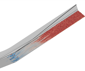
To make a closer comparison between the GSA and DNS, figure 10 presents the iso-surfaces of  $|w/U_\infty | = 0.006$ at $tU_\infty /L = 6$ in the exponential growth stage obtained from the DNS. Also shown in this figure are the contours of spanwise velocity in the $x$–
$x$– $y$ plane at $z/L = 0.14$ and the $z$–
$z$– $y$ plane at $x/L = 1.05$ at the same time instant. The spanwise velocity is mostly confined within the separation region with an average spanwise wavelength of 0.056, which agrees well with the GSA prediction.

Figure 10. (a) Iso-surfaces of  $w/U_\infty = -0.006$ (blue) and $w/U_\infty = 0.006$ (red) obtained from the DNS at the time instant $tU_\infty /L = 6$. The numerical schlieren is added at $z/L = 0$ to highlight the position of the separation bubble. (b–c) Instantaneous distribution of spanwise velocity ( $w/U_\infty$) at $tU_\infty /L = 6$ in the $x$–
$x$– $y$ plane at $z/L = 0.14$ and the $z$–
$z$– $y$ plane at $x/L = 1.05$. Closed circles in panel (b) mark the separation and reattachment positions.
For each eigenvalue, the GSA solver returns a normalised complex eigenfunction. A scaling factor can be determined by dividing the largest spanwise velocity in figure 10(c) by the largest magnitude of the spanwise velocity perturbation of the most unstable mode (i.e. mode 1 at  $\lambda _z/L = 0.055$) along a wall-normal slice at the same streamwise location. The eigenfunction of mode 1 is then multiplied by the scaling factor and extends to five periods in the spanwise direction to construct a 3-D perturbation field corresponding to $tU_\infty /L = 6$.
Figures 11(a) and 11(b) show the contours of the spanwise velocity perturbations in the  $x$–
$x$– $y$ plane at $z/L = 0.12$ and the $z$–
$z$– $y$ plane at $x/L = 1.05$, respectively. Note that the locations of the separation and reattachment points denoted by the closed circles are obtained from the 2-D base flow, which has a slightly smaller separation region than the 3-D saturated flow in the DNS. Figures 11(c) and 11(d) plot the iso-surfaces of the streamwise and spanwise velocity perturbations extracted from the 3-D perturbation field. The good agreement between the GSA and DNS confirms the validity of both methods. In contrast to $w'$,
$w'$,  $u'$ stretches downstream along the reattaching boundary layer, leading to spanwise alternating acceleration and deceleration in the streamwise direction. Similar behaviours were also observed by Hildebrand et al. (Reference Hildebrand, Dwivedi, Nichols, Jovanović and Candler2018) for an oblique-shock impingement on a flat plate.

Figure 11. (a,b) Contours of the spanwise velocity perturbations in the  $x$–
$x$– $y$ plane at $z/L = 0.12$ and $z$–
$z$– $y$ plane at $x/L = 1.05$. (c) Iso-surfaces of $|w'/U_\infty | = 0.006$. (d) Iso-surfaces of $|u'/U_\infty | = 0.015$. The perturbation field is constructed using the eigenfunction of mode 1 at $\lambda _z/L = 0.055$ with the amplitude corresponding to $tU_\infty /L = 6$.
The change in the flow topology due to the global instability can be examined by the linear superposition of the 2-D base flow and the 3-D perturbation field (Theofilis, Hein & Dallmann Reference Theofilis, Hein and Dallmann2000). At  $tU_\infty /L = 6$, the perturbation amplitude is not large enough to alter the reattached flow significantly, as shown in figure 3(a). Here, we focus on the topological change downstream of flow reattachment at $tU_\infty /L = 7$ by further amplifying the 3-D perturbation field according to (3.2) using the largest growth rate of mode 1. Figure 12 shows the contours of the perturbed streamwise velocities in three wall-normal planes extracted at $x/L = 1.27$, 1.45 and 1.60 superimposed with the in-plane streamlines. Note that only the regions with $0 \leqslant u/U_\infty \leqslant 0.92$ are displayed. Note also that $y_n$ denotes the wall-normal coordinate starting from the wall. The station with $x/L = 1.27$ is located immediately downstream of the 2-D reattachment point. However, the global instability induces local regions of reversed flow embedded in the reattaching boundary layer, which indicates that the reattachment line is no longer straight but has a zigzag pattern. The meandering reattachment line can also be observed in the saturated flow (see DNS results in figure 3). Meanwhile, the edge of the reattaching boundary layer becomes corrugated. At $x/L = 1.45$ and 1.60, streamwise vortices can be seen with the peak–valley structure corresponding to the upwash and downwash motions. The GSA confirms that streamwise vortices can be generated due to the global instability of the flow system, which can persist along the compression ramp and eventually break down into turbulence.

Figure 12. Contours of the perturbed streamwise velocities in three wall-normal planes extracted at (a)  $x/L = 1.27$, (b) $x/L = 1.45$ and (c) $x/L = 1.60$ superimposed with the in-plane streamlines. The perturbed flow field is constructed using the eigenfunction of mode 1 at $\lambda _z/L = 0.055$ with the amplitude corresponding to $tU_\infty /L = 7$. The cutoff levels are $u/U_\infty < 0$ and $u/U_\infty > 0.92$.
Although the linear GSA predicts the main flow features (e.g. spanwise periodicity, streamwise vortices) for the considered compression-ramp flow, there are certain nonlinear effects that are not revealed by the GSA. In fact, the DNS results indicate the occurrence of higher harmonic of spanwise wavelength. For instance, it can be estimated from figure 3(b,c) that the typical wavelength of heat-flux streaks is approximately  $\lambda _z / L = 0.027$. This value is approximately half of the wavelength of the most unstable global mode (mode 1). Figure 13 compares the spanwise velocity fields obtained from the DNS at $tU_\infty /L = 6$ and $tU_\infty /L = 7.2$. Note again that the linear growth stage ends at $tU_\infty /L = 6.5$. The streamwise position is $x/L = 1.15$ for figure 13(a–b) and $x/L = 1.27$ (reattachment position) for figure 13(c–d). It is clear that only mode 1 is present at $tU_\infty /L = 6$. However, a new mode occurs near the wall after the linear growth stage. As a result, the spanwise wavelength is doubled near the wall. To further examine the streamwise location of this mode, a fast Fourier transform for the spanwise velocity fields on a wall-parallel plane ( $y_n / L = 0.0015$) at $tU_\infty /L = 6$ and 7.2 is carried out. The resulting power spectral density (PSD) contours as a function of spanwise wavelength and streamwise location are presented in figure 14. Obviously, the dominant wavelength at $tU_\infty /L = 6$ is in the range $\lambda _z / L = 0.05 {\sim} 0.06$, corresponding to mode 1. At $tU_\infty /L = 7.2$, however, another high-energy mode can be found at $\lambda _z / L = 0.027$, which corresponds to the second harmonic of mode 1. Moreover, the second harmonic extends further downstream of reattachment, while mode 1 is mainly confined in the separation bubble. This means that the second harmonic dominates the spanwise periodicity in the near-wall region downstream of reattachment. This explains the observed wavelength of surface heat-flux streaks in the saturated flow.

Figure 13. Instantaneous distributions of spanwise velocity on the  $z$–
$z$– $y$ planes at (a–b) $x/L = 1.15$ and (c–d) $x/L = 1.27$. The time instants are (a,c) $tU_\infty /L = 6$, (b,d) $tU_\infty /L = 7.2$.

Figure 14. Power spectral density of the spanwise velocity on a wall-parallel plane ( $y_n/L = 0.0015$) at (a) $tU_\infty /L = 6$ and (b) $tU_\infty /L = 7.2$.
4. Transition to turbulence downstream of reattachment
4.1. Influence of low-frequency unsteadiness
The oscillatory unstable modes revealed by the GSA imply the presence of unsteady flow. According to the DNS results, the saturated flow exhibits a strong unsteadiness both inside and downstream of the separation bubble. For a similar compression-ramp flow with a lower Reynolds number, Cao et al. (Reference Cao, Hao, Klioutchnikov, Olivier and Wen2021b) demonstrated that the flow unsteadiness can be attributed to the intrinsic instability of the flow system. With this view, the flow unsteadiness and its effects on the transition process are first addressed in this section.
To facilitate the following discussion, it is necessary to highlight some critical positions in the flow field. Figure 15 shows the time-averaged wall Stanton number on the ramp and marks several positions; C denotes the corner ( $x/L = 1$); R corresponds to the spanwise-averaged reattachment position ( $x/L = 1.27$); P represents the peak-heating position ( $x/L = 1.45$) and T indicates the onset of transition ( $x/L = 1.76$, estimated from figure 4b).

Figure 15. Contour of the time-averaged wall Stanton number. Here, C denotes the corner ( $x/L = 1$), R corresponds to the spanwise-averaged reattachment position ( $x/L = 1.27$), P represents the peak-heating position ( $x/L = 1.45$) and T indicates the onset of transition.
Figure 16(a) presents the temporal history of the reattachment position ( $x_R$) in the centre line of the wall, in comparison with the wall Stanton number signal shown in figure 2(b). In general, there exists an opposite trend for the two signals. When the reattachment position moves downstream, the Stanton number decreases, and vice versa. This is consistent with the results of Cao et al. (Reference Cao, Hao, Klioutchnikov, Olivier and Wen2021b), who found that the pulsation of the reattachment position is accompanied by the variation of downstream surface heat flux. Figure 16(b) compares the temporal history of the wall Stanton number and the boundary-layer displacement thickness ( $\delta _1$) at the same position ( $x/L = 1.45, z/L = 0.15$). Similar to figure 16(a), a generally opposite trend can also be observed. In other words, a high heat flux on the wall corresponds to a thin boundary layer above this position, and vice versa. This is not surprising because the thinning of the boundary layer induces a high temperature gradient on the cold wall. Concerning the spatial distribution of the surface heat flux, its streak pattern indicates that there exist streamwise-elongated high- and low-momentum streaks for the boundary layer above the wall. Therefore, like the surface heat-flux streaks, the boundary-layer streaks also exhibit an unsteady feature. The complicated spatio-temporal distribution of the reattached boundary layer has a significant influence on the transition process, as is shown later.

Figure 16. (a) Temporal history of the reattachment position (solid line) in the centre line of the wall ( $z/L = 0.15$), in comparison with the wall Stanton number signal (dash dotted line) at $x/L = 1.45$, $z/L = 0.15$ (extracted from figure 2b). (b) Temporal history of the boundary-layer displacement thickness (solid line) and wall Stanton number signal (dash dotted line) at $x/L = 1.45$ and $z/L = 0.15$.
To characterise the streamwise propagation of the unsteadiness, a two-point spatio-temporal correlation is employed to evaluate the wall Stanton number signal
 \begin{equation} R_{nm}(\tau)=\frac{\overline{St'_{n}(t)\cdot St'_{m}(t+\tau)}}{\sqrt{\overline{St'^{2}_{n}}} \cdot \sqrt{\overline{St'^{2}_{m}}}}, \end{equation}
where the subscript  $n$ denotes the reference point: $x/L = 1.6$, $z/L = 0.15$; the subscript $m$ corresponds to the position varying in the streamwise or spanwise direction; $St' = St-\overline {St}$ is the fluctuation quantity ( $\overline {St}$ is the time-averaged $St$ at local streamwise or spanwise position) and $\tau$ is the time delay. The resulting correlation maps are shown in figure 17. The vertical coordinates are given by $\Delta x = x/L - 1.6$ and $\Delta z = z/L - 0.15$. A strong correlation is found in the streamwise direction, whereas the correlation in the spanwise direction is quite weak. This means that the unsteadiness primarily travels in the streamwise direction. The slope of the black line shown in figure 17(a) indicates the travelling speed of the unsteadiness, which is evaluated approximately by $0.5U_\infty$.

Figure 17. Two-point temporal correlation map of the wall Stanton number in the (a) streamwise and (b) spanwise directions. The reference point is located at  $x/L = 1.60$, $z/L = 0.15$.
Figure 18 presents the PSD of the wall Stanton number signal shown in figure 16 as well as the spanwise-averaged PSD at  $x/L = 1.45$. Welch's method (Welch Reference Welch1967) is employed for the spectral estimation with three segments and 50 % overlap. A Hamming window is used for weighting the data on each segment prior to fast Fourier transform processing. The above setting yields the length of an individual segment as $12.5L/U_\infty$. It is apparent that the wall Stanton number signal has a broadband low-frequency feature. The dominant non-dimensional frequencies (Strouhal number) are of the order of 0.1. The spanwise-averaged PSD has a similar distribution to the PSD at $z/L = 0.15$, which indicates that the dominant frequencies at different spanwise positions are nearly the same.

Figure 18. PSD of the wall Stanton number signal shown in figure 16 (solid line) and the spanwise-averaged PSD (dash dotted line) at  $x/L = 1.45$.
The influence of low-frequency unsteadiness on the transition process can be further illustrated by showing the wall pressure signal at different streamwise positions in figure 19. The chosen positions are  $x/L = 1.45$, 1.80, 2.10 and 3.00 along the centre line of the wall. As seen, no high-frequency fluctuation exists at $x/L = 1.45$, indicating a laminar state for the boundary layer. At $x/L = 1.80$, high-frequency fluctuation packets intermittently occur in the pressure signal. By roughly counting the number of fluctuation packets, the frequency for the occurrence of a packet is approximately $fL/U_\infty = 7/25 = 0.28$, which is consistent with the typical frequency of the flow unsteadiness (see figure 18). At $x/L = 2.10$, the pressure signal exhibits a high-frequency feature at most time instants, although the intermittent appearance of fluctuation packets is still present. This means that the flow is highly transitional here. A turbulent boundary layer at $x/L = 3.00$ is indicated by the pressure signal shown in figure 19(d).

Figure 19. Temporal history of the wall pressure at different streamwise positions along the centre line of the wall. (a–d) Correspond to the signal at  $x/L = 1.45$, 1.80, 2.10 and 3.00.
4.2. Breakdown of streamwise vortices
As mentioned previously, the unsteady heat-flux streaks on the wall are the footprint of unsteady boundary-layer streaks above the wall, and the unsteadiness can be traced back to the reattaching flow. The streak pattern for the reattached boundary layer is further visualised in the following. Figure 20 illustrates the streamwise velocity contour ( $u/U_\infty$) in the wall-normal plane at $x/L = 1.27$, 1.35, 1.45, 1.50 and 1.60 for the time instant $tU_\infty /L = 41$ superimposed with the in-plane streamlines. Note that the contour outside the boundary layer is removed by cutting off the levels of $u/U_\infty > 0.92$. As $x/L = 1.27$ is the spanwise-averaged reattachment position, both reverse and reattached flows are present in figure 20(a). Downstream of reattachment (figure 20b–e), the distorted boundary layer exhibits spanwise corrugation, and the high- and low-momentum portions persist in the streamwise direction. This is consistent with previous GSA predictions (see figures 11 and 12). Therefore, it is concluded that the occurrence of streamwise-elongated boundary-layer streaks is triggered by the intrinsic instability in the flow system.

Figure 20. Instantaneous ( $tU_\infty /L = 41$) streamwise velocity contour in the wall-normal plane at different streamwise positions superimposed with in-plane streamlines. (a–e) Correspond to $x/L = 1.27$, 1.35, 1.45, 1.50 and 1.60, respectively. The cutoff levels are $u/U_\infty < 0$ and $u/U_\infty > 0.92$.
Further evidence can be found by comparing the in-plane streamlines in figures 12 and 20. It is apparent that counter-rotating vortices are present downstream of reattachment. Between two adjacent vortex pairs, the boundary layer is compressed towards the wall, causing a large temperature gradient and thus a hot region on the wall. At the centre of a vortex pair, the upwash motion brings low-momentum flow away from the wall, producing a cold region on the wall. It should be mentioned that the change in the flow direction at the upper side of both figures 12 and 20 is induced by the flow reattachment and downstream growth of the boundary layer. The consistent vortical structure between the GSA and DNS results indicates that the global instability plays an important role in the formation of streamwise vortices and heat-flux streaks. It is further noted that there are three distinct vortex pairs in figure 20, whereas only one and a half vortex pairs can be observed in figure 12. In other words, the number of vortices or streaks in the saturated flow (DNS data) is twice of that in the flow governed by the linear instability (GSA data). This is due to the emergence of the second harmonic of the most unstable mode, as discussed previously.
To visualise the breakdown of the streamwise vortices, the instantaneous distribution of streamwise vorticity on the wall-parallel plane at  $y_n/L = 0.005$ is shown in figure 21. The streamwise vorticity is defined as
 \begin{equation} \omega_s = \frac{\partial w}{\partial y_n} - \frac{\partial u_n}{\partial z}, \end{equation}
where  $u_n$ denotes the wall-normal velocity component. Owing to the flow unsteadiness, the distributions of $\omega _s$ at $tU_\infty /L = 40$ and 41 differ from each other. The boundary layer tends to be homogeneous upstream of $x/L = 2.3$ at $tU_\infty /L = 41$, whereas it is still transitional up to $x/L = 2.5$ at $tU_\infty /L = 40$. In general, the typical breakdown position can be estimated at $x/L = 1.7 {\sim} 1.8$, which is consistent with the aforementioned position for the onset of transition (see figure 4). On the other hand, the streak patterns at the two time instants share some similarities. For example, the evolution of the streamwise streaks in both figures starts from the reattachment region (around $x/L = 1.27$). Moreover, each streak consists of a vorticity pair, which represents a pair of counter-rotating vortices.

Figure 21. Instantaneous distribution of the streamwise vorticity ( $\omega _s$, non-dimensional) on the wall-parallel plane at $y_n/L = 0.005$ for the time instants (a) $tU_\infty /L = 40$ and (b) $tU_\infty /L = 41$.
Subsequently, the  $Q$-criterion is employed to visualise the flow structures, Q is the second invariant of the velocity gradient tensor. As shown in figure 22, the vortical structure originates from the separation bubble flow and evolves in the streamwise direction. Affected by the flow unsteadiness, the onset of transition differs for each streamwise vortical streak. Interestingly, vortical structures with a ‘hairpin’ shape can be observed in the transitional region (see the enlarged views in figure 22b,d). This structure resembles the varicose mode of streak breakdown in a flat-plate boundary layer (Ovchinnikov, Choudhari & Piomelli Reference Ovchinnikov, Choudhari and Piomelli2008; Schlatter et al. Reference Schlatter, Brandt, De Lange and Henningson2008). In short, the above facts demonstrate that the transition process in the considered compression-ramp flow is initiated by its intrinsic instability and accomplished via the breakdown of streamwise vortices.

Figure 22. Instantaneous visualisation of the vortical structure on the basis of the  $Q$-criterion. The iso-surface of $Q = 50$ coloured by the velocity magnitude $U = \sqrt {u^2 + v^2 + w^2}$ is shown in all panels. Panels (b,d) are enlarged views of panels (a,c), respectively. The time instant is $tU_\infty /L = 40$ for (a–b) and $tU_\infty /L = 41$ for (c–d). Numerical schlieren is added to highlight the separation bubble and shock structure.
5. Conclusion
In the present work, DNS and GSA were performed for a hypersonic compression-ramp flow, where the transition to turbulence has been detected in shock tunnel experiments. The free-stream Mach number and the Reynolds number based on the flat-plate length are 7.7 and  $8.6 \times 10^5$, respectively. Owing to the strong SWBLI, a large separation bubble forms around the corner. Without introducing any external disturbances to the DNS, the flow system was shown to be intrinsically unstable, causing the formation of surface heat-flux streaks and the transition to turbulence downstream of reattachment. The DNS results were verified using experimental data and theoretical predictions.
The global stability of the 2-D base flow was examined by the GSA. Three stationary and seven oscillatory unstable modes were revealed. The most unstable mode is a stationary one with its growth rate peaking at the spanwise wavelength  $\lambda _z/L = 0.055$. This mode dominates the linear growth stage in the DNS. The frequency of the oscillatory modes ( $fL/U_\infty$) ranges from 0.474 to 1.668. By superimposing the 3-D perturbation field of the most unstable mode on the base flow, a spanwise corrugation of the reattaching shear layer and reattached boundary layer was uncovered, accompanied by the formation of streamwise vortices. Similar structures were extracted from the DNS results. The comparison between the DNS and GSA results demonstrated that the occurrence of streamwise boundary-layer streaks and streamwise vortices downstream of reattachment is triggered by the intrinsic instability in the flow system.
In addition, the DNS results indicated the occurrence of the second harmonic of the most unstable global mode, which was not revealed by the linear GSA. It was shown that the second harmonic dominates the spanwise periodicity in near-wall shear flows after flow saturation. As a result, the spanwise wavelength of streamwise vortices and surface heat-flux streaks in the saturated flow is approximately half of the most unstable mode predicted by the GSA. Consistent with the result of Cao et al. (Reference Cao, Hao, Klioutchnikov, Olivier and Wen2021b), the saturated flow exhibits a broadband low-frequency unsteadiness. The boundary-layer streaks and surface heat-flux streaks mainly oscillate in the streamwise direction with a typical Strouhal number of the order of 0.1. This unsteadiness has a significant influence on the transition process. For example, the transition length exhibits a temporal-spatial dependence. It was shown that the transition to turbulence starts from the breakdown of streamwise vortices. Hairpin vortical structures were identified in the transitioning flow.
It is interesting to note that self-excited instability is ubiquitous in separated flows involving SWBLI. Examples are compression-ramp flow (Egorov, Neiland & Shredchenko Reference Egorov, Neiland and Shredchenko2011; Sidharth et al. Reference Sidharth, Dwivedi, Candler and Nichols2017), shock impingement on a flat plate (Robinet Reference Robinet2007; Nichols et al. Reference Nichols, Larsson, Bernardini and Pirozzoli2017), double-wedge flow (Sidharth et al. Reference Sidharth, Dwivedi, Candler and Nichols2018), double-cone flow (Hao et al. Reference Hao, Fan, Cao and Wen2022) and flow over a hollow cylinder/flare (Brown et al. Reference Brown, Boyce, Mudford and O'Byrne2009; Lugrin et al. Reference Lugrin, Beneddine, Garnier and Bur2021a). Both stationary and oscillatory global modes were revealed using GSA (see, e.g. Nichols et al. Reference Nichols, Larsson, Bernardini and Pirozzoli2017; Sidharth et al. Reference Sidharth, Dwivedi, Candler and Nichols2018; Hao et al. Reference Hao, Fan, Cao and Wen2022). The formation of streamwise streaks and low-frequency unsteadiness in such flows are closely linked to the intrinsic instability. Hence, intrinsic instability provides a viable scenario for the transition to turbulence in separated flows, as highlighted in the present study.
However, in an intrinsically stable flow, the convective mechanism can dominate the formation of streamwise streaks, as shown by Dwivedi et al. (Reference Dwivedi, Sidharth, Nichols, Candler and Jovanović2019). As the introduction of upstream disturbances is inevitable in high-speed wind tunnel experiments, both intrinsic and convective instabilities may play a role. Because the numerical and experimental results in the present study agree well, it might be possible that the experimental flow is dominated by the intrinsic instability. Nevertheless, the influence of upstream disturbances on the formation of streamwise streaks and transition process in the considered flow needs to be further investigated. A comprehensive study of the combined effects of intrinsic and convective instabilities on SWBLI contributes to the understanding of transition in experiments and flight tests.
Funding
This work was jointly supported by RWTH Aachen University and the Hong Kong Research Grants Council (no. 25203721). The authors gratefully acknowledge the computing time granted by the JARA Vergabegremium and provided on the JARA Partition part of the supercomputer CLAIX at RWTH Aachen University under project JARA0218.
Declaration of interests
The authors report no conflict of interest.
Appendix. Shape of GSA modes 1 and 2 at  $\lambda _z/L = 0.055$

Figure 23 presents the spatial structure of modes 1 and 2 at  $\lambda _z/L = 0.055$ constructed by the real parts of different perturbation variables.

Figure 23. Shape of (a–f) mode 1 and (g–l) mode 2 at  $\lambda _z/L = 0.055$ coloured by the real parts of different perturbation variables. The contour levels are evenly spaced between $\pm$0.1 of the maximum amplitude.


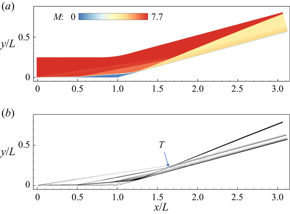


 Open access