2.1. Facility overview

All experiments were performed in HyperTERP, a small-scale reflected shock tunnel operated by the University of Maryland. A contoured Mach-5.95 nozzle with a $22$ cm exit diameter was employed, exhausting into a $30.5$ cm diameter free-jet test section equipped with $15.2$ cm diameter windows. A more detailed description of the facility is given in Butler & Laurence (Reference Butler and Laurence2019). The total specific enthalpy was held approximately constant at $0.89$ MJ kg$^{-1}$, corresponding to a temperature of $890$ K, with unit Reynolds numbers, $Re_m=\rho _\infty U_\infty /\mu _\infty$, of $3.33$, $4.49$ and $5.24\times 10^6\ {\rm m}^{-1}$ achieved by varying the reservoir pressure (viscosity is calculated here using Sutherland's law). Reference reservoir (subscript 0) and corresponding free stream properties (subscript $\infty$) for each condition are detailed in table 1; the methodology used to calculate these conditions and an overview of the free stream characterization are given in Butler & Laurence (Reference Butler and Laurence2021b). Typical reservoir pressure traces for all conditions are provided in figure 1. In each case, the steady test time is approximately $6$ ms, during which the unsteadiness in pressure is of the order of 2 % (standard deviation). Note that runs at condition Re52 are often affected by spikes in pressure (e.g. at $t\approx 6$ ms in figure 1) which must dissipate before data reduction. Shot-to-shot variation in the mean pressure is of the order of 1.3 %, while systematic uncertainty (combined calibration and nonlinearity) is estimated as 1.6 %. Shock-speed estimates are accurate to $\pm 5\ {\rm m}\ {\rm s}^{-1}$, contributing 0.4 % uncertainty in the reservoir temperature.

Table 1. Typical HyperTERP test conditions for this investigation.

Figure 1. Sample reservoir pressure traces at each condition.

2.2. Test article and instrumentation

The test article for this study was a cone/flare model comprising a 5$^\circ$ half-angle, stainless steel frustum of $410$ mm length and interchangeable, $76.2$ mm long, Delrin flares. Flare half-angles of 5$^\circ$, 10$^\circ$, 15$^\circ$ and 20$^\circ$ were employed, corresponding to a straight continuation of the frustum surface and compression angles of +5$^\circ$, +10$^\circ$ and +15$^\circ$. The model with the +10$^\circ$ configuration is pictured in figure 2. The nose radius was measured to be $0.10$ mm using a SmartScope optical gauge. The straight-cone configuration was included to provide comparisons against an undisturbed boundary layer.

Figure 2. Model schematic for the +10$^\circ$ configuration showing the sensor layout; all dimensions are in millimetres.

A single streamwise row of PCB 132B38 pressure transducers was installed along the upper surface of the cone, held in place using clear nail polish (Ort & Dosch Reference Ort and Dosch2019). The sensor locations are indicated in figure 2, and corresponding distances along the cone surface from the nosetip are provided in table 2. These sensors were sampled at 2 MHz with a 600 kHz low-pass filter to remove aliasing effects. The factory-supplied calibration was used in converting the voltage signals to pressure, though this does not account for the varying frequency response of the sensors (Ort & Dosch Reference Ort and Dosch2019). It should additionally be noted that Ort & Dosch (Reference Ort and Dosch2019) observed parasitic resonances at frequencies above 300 kHz for this sensor model and corresponding peaks were observed in many of the spectra in the present experiments; results near this frequency should thus be treated with caution. To analyse the pressure-disturbance data, average power spectral densities (PSDs) were computed over the steady test duration using Welch's method with Hann windows of length 128. Disturbance $N$ factors, i.e. the spatial integral of the amplification rate, could be computed for each frequency according to

(2.1)\begin{equation} \Delta N(f,x_i) = \frac{1}{2}\ln \left( \frac{PSD(f,x_i)}{PSD(f,x_0)} \right),\end{equation}

where $PSD(f,x_i)$ refers to the power of frequency $f$ at streamwise location $x_i$ and $x_0$ refers to the most upstream station. Similarly, the maximum second-mode $N$ factor could be computed by instead considering only the peak PSD within the frequency range of the second mode at each station.

Table 2. Surface coordinates of PCB stations.

The model was initially installed at approximately zero incidence (pitch and yaw) with the aid of a laser level by aligning the model seam and PCB array with the horizontal and vertical centrelines of the nozzle. To further refine the model pitch, measurements were also performed with an additional PCB sensor installed on the underside of the model opposite station U1, as second-mode frequencies are known to be highly sensitive to angle-of-attack variations. From these measurements, it was determined that the pitch angle was less than 0.2$^\circ$, with any residual offset corresponding to the upper ray of the model (where measurements were performed) lying on the flow-leeward side. Although no comparable measurements were made regarding model yaw, small yaw variations are expected to have a negligible effect on the flow behaviour in the region of interest.

2.3. Calibrated schlieren

High-speed flow field visualization, obtained using a standard Z-type schlieren with a horizontal knife edge, serves as the primary means of flow interrogation throughout this work. Light pulses of $20$ ns duration were provided by a Cavilux HF laser and a Phantom v2512 camera was used to capture the images at frame rates between $440$ kHz and $822$ kHz (the lower frame rate being used for the larger flare angle), allowing resolution of spectral content up to $411$ kHz. The frame rates were chosen to be higher than the Nyquist sampling rate of the dominant boundary-layer disturbances (typically second-mode waves). The field of view ranged from $512\times 32$ pixels at $822$ kHz to $640\times 64$ pixels at $440$ kHz, with the camera rotated to maximize the region of flow visualized. The magnification of the optical set-up resulted in a length scale of 0.115 mm pixel$^{-1}$ for the +15$^\circ$ configuration and 0.139 mm pixel$^{-1}$ for all others. The theoretical, undisturbed boundary-layer thickness at the corner junction, $\delta _c$, ranged from $1.4\unicode{x2013}1.8$ mm depending on the condition (particular values are provided in table 1). This gives a visualized boundary-layer resolution of at least 10 pixels, though it should be noted that this number will be lower far upstream of the corner and along the compression flares due to the reduced boundary-layer thicknesses there.

The pixel intensities in each image were converted to integrated density gradients using the calibration procedure described by Hargather & Settles (Reference Hargather and Settles2012) and Kennedy (Reference Kennedy2019). A plano-convex, spherical lens (focal length 10 m, diameter 25.4 mm) with a known deflection angle profile was placed into the field of view and a reference image captured. The intensity profile along the lens face was then mapped to the known deflection profile, assuming zero deflection to correspond to 92 % of the background pixel intensity (to account for the 8 % absorption specific to the calibration lens). For a weak lens, the deflection angle, $\epsilon$, is given as a function of radial distance from the lens centre, $r$, by

(2.2)\begin{equation} r/f = \tan\epsilon \approx \epsilon.\end{equation}

The deflection profile is then mapped to the density gradient of the test gas according to

(2.3)\begin{equation} \epsilon = \frac{\kappa L}{n_\infty}\frac{\partial \rho}{\partial y}, \end{equation}

where $L$ is the integration path length of the light, $\kappa$ is the Gladstone–Dale constant, $\rho$ refers to the gas density, $y$ is the direction normal to the knife edge and $n_\infty$ is the index of refraction of air at laboratory conditions. Note that this formulation assumes the density gradient profile to be constant over the integration path; if this is not the case, the term $L\partial \rho /\partial y$ should be replaced by a corresponding integral.

The ultra-high frame rate employed throughout this work allows us to perform spectral analysis on the schlieren data without assuming a propagation speed for the disturbances (as was necessary, for example, in Kennedy et al. Reference Kennedy, Laurence, Smith and Marineau2018). To this end, after converting each image over the steady test duration into a map of density gradient using (2.3), PSD curves were computed for each pixel in the field of view using Welch's method with Hann windows of length 64. This process then allows us to visualize the spatial distribution of frequency content anywhere within the field of view. The number of frames included in these calculations varied from 2400 to 6000 (75 to 187 realizations), depending on the frame rate of the test. The one exception to this is the condition Re45 test of the +15$^\circ$ configuration. The latter half of this test was contaminated by anomalous turbulence and, thus, only 1300 images were kept. For reference, the exact number of frames used for each test is reported later in this article in table 4.

3.1. Straight (+0$^\circ$) continuation

We begin by examining the behaviour of the undisturbed boundary layer in the +0$^\circ$ configuration through the time-resolved schlieren sequences presented in figures 3 (condition Re33) and 4 (condition Re52). Exemplary schlieren sequences from combinations of flow condition and flare angle not provided here in the main article are included for reference in the online supplementary material (available at https://doi.org/10.1017/jfm.2022.769), together with animations of selected combinations. The images have been rotated to align the abscissa with the frustum and $X$ refers to the distance along the cone surface from the nose tip. At the top of each sequence is shown an average flow-on image to highlight the mean boundary-layer profile. Subsequent images are reference subtracted using a 40 image sliding average (corresponding to time intervals of between 49 and $91\ \mathrm {\mu }$s, depending on the frame rate) to emphasize transient features. Red triangles in the mean flow image denote the locations of PCB sensors, while red bars are used to bracket regions of interest and approximate the propagation of the disturbances as determined visually. Mean PSDs for select PCB sensors at each condition are presented in figure 5.

Figure 3. Reference-subtracted image sequence captured for the $+0^\circ$ configuration at condition Re33; the inter-image spacing, $\Delta t$, is $9.7\ \mathrm {\mu }$s.

Figure 4. Reference-subtracted image sequence captured for the +0$^\circ$ configuration at condition Re52; $\Delta t = 10.2\ \mathrm {\mu }$s.

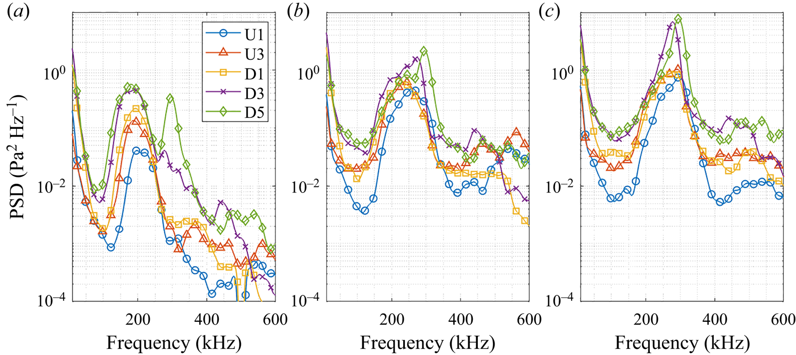
Figure 5. Power spectral densities at select PCB stations for the +0$^\circ$ configuration at (a) condition Re33, (b) condition Re45 and (c) condition Re52.

In the first reference-subtracted image of figure 3, distinct, rope-like waves are seen upstream of U3, revealing the presence of a second-mode wavepacket, with an additional wavepacket visible in the vicinity of D3. The upstream wavepacket then appears to intensify as it propagates along the cone surface, and the last three images of the sequence show distortions to its regular, periodic structure, which we interpret as an initial sign of breakdown, i.e. the precursor of transition. While this schlieren sequence is intended to be representative of the overall observed behaviour, the transition process in such conventional facilities is stochastic by nature and there is occasionally significant variation in wavepacket behaviour, with some breaking down over the frustum and others traversing the entire cone surface without showing obvious distortions to their structure.

The PCB spectra shed additional light on these qualitative trends (it should be emphasized that these spectra are representative of the average behaviour, rather than the isolated phenomena revealed in the images). Between U1 and U3, the peak second-mode frequency decreases from approximately $210$ kHz to $190$ kHz while the maximum $N$ factor increases by 0.6. Additional amplification is observed up to D3, where the maximum $N$ factor has increased by an additional 0.6. The deterioration of the wavepacket features downstream aligns with the amplitude saturation and spectral broadening observed in the spectra for sensors D3 and D5. Note that the $300$ kHz peak at station D5 is likely an example of anomalous sensor resonance and not attributable to flow features.

Wavepackets at condition Re52 almost universally exhibit transitional behaviour, which we interpret here to correspond to a clear loss of the regular, periodic structures observed upstream and the onset of a more chaotic, disordered appearance; this is exemplified in figure 4. The highlighted wavepacket in this sequence breaks down as it reaches $X=400$ mm, resulting in what appears to be a young turbulent spot over much of the extension. The PCB spectra indicate that mean saturation occurs between U1 and U3, as the fundamental peak (now at $280$ kHz) experiences no growth while surrounding frequencies amplify by nearly an order of magnitude. This spectral broadening continues along the length of the model, though the second-mode peak is still apparent at D5, indicating that (on average) the boundary layer is not yet in a fully developed turbulent state. The sensor resonance in D3 and D5 now overlaps with the second-mode peak however, making it difficult to discern the true amplitude of the disturbances (again, the strong resonance peak near $300$ kHz should be ignored as unphysical). The behaviour of the boundary-layer disturbances at condition Re45 generally lies between what has been presented for conditions Re33 and Re52, with a decrease in second-mode amplitude between sensors D3 and D5 indicating saturation early on the cone extension.

3.2. The +5$^\circ$ flare

When compared with the straight extension, the +5$^\circ$ compression flare serves largely to promote disturbance growth and transition. Figure 6 presents an image sequence captured at condition Re45 with the +5$^\circ$ configuration, again concentrating on an incoming second-mode wavepacket. The field of view for this test is focused primarily on the flare to better capture the downstream development of the boundary-layer disturbances. First, from the mean image, we note that the boundary layer appears fully attached at the corner. When the wavepacket encounters the SWBLI, transient flow structures are radiated away along the expected location of the corner shock (though the shock itself is too weak to be clearly visible): this is indicated by the red arrow in the fourth and fifth images of the sequence. This radiation, apparent for nearly all wavepackets, has a periodicity similar to the second-mode structures and typically appears to emanate from the tail of a wavepacket (this is most clearly seen in movie 1, provided in the online supplementary material). Similar radiation of disturbance energy along weak, mean flow discontinuities appeared in computations performed by Sawaya et al. (Reference Sawaya, Sassanis, Yassir and Sescu2018) of second-mode waves interacting with two-dimensional wall deformations. Downstream of the corner the wavepackets retain their rope-like appearance, but the structure angle of the disturbances decreases such that they appear more parallel to the model surface. In the schlieren sequence, the tail of the wavepacket shows signs of breakdown around $X=440$ mm. This occurs as the head of the packet, which has maintained its periodic structure, is leaving the field of view.

Figure 6. Reference-subtracted image sequence captured for the +5$^\circ$ configuration at condition Re45; $\Delta t = 7.3\ \mathrm {\mu }$s.

Amplification of the second mode is seen in the PCB spectra of figure 7(b) until station D3, similar to the straight extension at this condition (Re45). Importantly, however, the broadband amplification observed between sensors D1 and D3 exceeds that of the +0$^\circ$ configuration, implying an overall acceleration of the transition process relative to the undisturbed boundary layer. We also note that the PCB spectra along the flare, particularly D3 and D5, demonstrate a shift in the second-mode peak to higher frequencies consistent with the reduced boundary-layer thickness.

Figure 7. Power spectral densities for select PCB stations at the +5$^\circ$ configuration at (a) condition Re33, (b) condition Re45 and (c) condition Re52.

The behaviour just described for the Re45 condition is also generally representative of condition Re33, though the boundary layer is less transitional along the flare at the lower $Re_m$. This is evident from the reduced spectral broadening seen in the PCB spectra in figure 7(a). At condition Re52 (rightmost plot of figure 7), the PCB spectra along the flare (D1, D3 and D5) show significant amplification in frequencies above and below the second-mode peak. It is unclear to what extent the spike in second-mode power at D3 and D5 is caused by sensor resonance, but in any case, the signal has become largely broadband along the flare, indicative of the onset of a young turbulent boundary layer. Indeed, the full test video shows this to be typically the case, with many wavepackets already breaking down upstream of the flare. When contrasted with the straight-cone case, the results here indicate that the attached SWBLI here accelerates boundary-layer transition for unit Reynolds numbers above that of condition Re33.

3.3. The +10$^\circ$ flare

The development of second-mode wavepackets encountering the +10$^\circ$ flare was reviewed in detail by Butler & Laurence (Reference Butler and Laurence2021a). The adverse pressure gradient imposed by this compression is sufficient to separate the boundary layer upstream of the flare for all Reynolds numbers considered. Approximate separation and reattachment locations were identified as points at which the pseudo-streamline profiles reported in § 4 exhibited a sudden change in slope; reasonable agreement (to within $2$ mm) was obtained between these results and preliminary numerical simulations (Butler Reference Butler2021). These locations are represented in each image sequence by vertical, dashed lines and are given in table 3; the uncertainty in each location is estimated as $\pm 3$ mm.

Table 3. Approximate separation and reattachment locations for the +10$^\circ$ and +15$^\circ$ configurations.

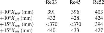
Figure 8 depicts the typical transitional behaviour of wavepackets which encounter the separated region at condition Re45; a corresponding movie, movie 2, is provided in the online supplementary material. In the mean image, the boundary layer separates between sensor U3 and the corner junction, and reattaches in the vicinity of D3. At the separation point, the instability waves lift off the cone surface and propagate largely within the separated shear layer. The incoming wavepacket can be seen to undergo substantial morphing downstream of separation, with some features propagating near the wall within the recirculation zone. As in the +5$^\circ$ case, periodic structures are radiated away when the wavepacket encounters the SWBLI (highlighted by red arrows in the second, third and fourth images of the sequence); however, this now occurs along the expected location of the separation shock. Downstream of reattachment the packet's structure has become distorted and retained little of its ‘rope-like’ appearance. Such behaviour is not fully representative of condition Re45 however, as the state of the incoming wavepacket may substantially alter its development through the SWBLI. In the first image of the sequence in figure 8, for example, a wavepacket is visible downstream of D3 that has largely retained its structure. The latter behaviour is more representative of wavepackets seen at condition Re33.

Figure 8. Reference-subtracted image sequence captured for the +10$^\circ$ flare at condition Re45; $\Delta t = 9.7\ \mathrm {\mu }$s. The dashed vertical lines indicate the approximate separation and reattachment locations.

Beyond the clear second-mode signature upstream of separation (sensors U1 and U3) in the middle image of figure 9, there is evidence of a harmonic developing in the U3 spectra at $500$ kHz (a phenomenon also seen at Re33 around $440$ kHz). Sensor D1 shows a marked decrease in second-mode power, which may reflect the tendency for the disturbances to lift off the surface; note also, however, the increase in low-frequency content relative to sensor U3, peaking at $85$ kHz. A similar peak is seen around $73$ kHz at condition Re33 and we have demonstrated previously that these lower-frequency spectral features correspond to distinct, shear-layer disturbances (Butler & Laurence Reference Butler and Laurence2021a). The increasingly broadband nature of the spectra of sensors D3 and D5 match the transitional behaviour generally observed in images. At condition Re52, the separation region has shrunk significantly and the instantaneous flow structures on the flare are generally distorted and chaotic in appearance. This is also reflected in the PCB spectra, where even sensor D1 exhibits primarily broadband content.

Figure 9. Representative PSDs at select PCB stations for the +10$^\circ$ configuration at (a) condition Re33, (b) condition Re45 and (c) condition Re52.

3.4. The +15$^\circ$ flare

As evident from the mean flow-on image in figure 10 (captured at condition Re45), the +15$^\circ$ compression flare produces a large separation bubble which at conditions Re33 and Re45 extends far enough upstream to fully envelop sensor U3. Approximate separation and reattachment locations for this configuration are given in table 3. These were determined in the same manner as previously, though the separation location could not be determined at conditions Re33 and Re45 as the boundary layer appeared to separate upstream of the field of view in both cases.

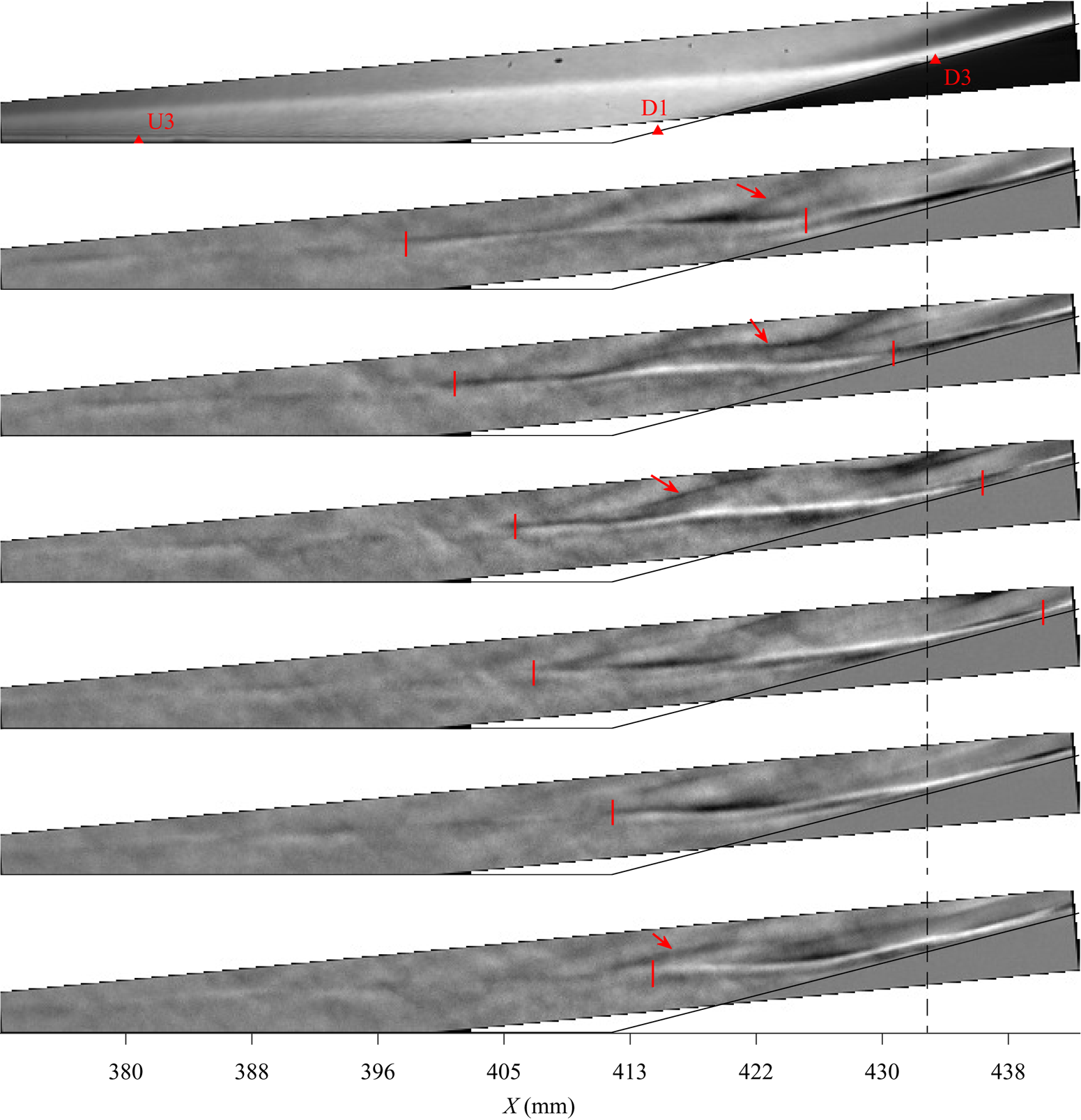
Figure 10. Reference-subtracted image sequence captured for the +15$^\circ$ configuration at condition Re45; $\Delta t = 5.5\ \mathrm {\mu }$s. The dashed vertical line indicates the approximate reattachment location.

For conditions Re33 and Re45, second-mode wavepackets appear only intermittently within the field of view for this flare angle (note that this also made it difficult to define a pseudo-streamline, which will lead to additional uncertainty in the reattachment location) and the dominant transient phenomenon instead appears to be shear-layer disturbances that originate over the separation bubble. These disturbances manifest themselves as long, wavy structures primarily aligned with the direction of propagation: an example may be seen in the instantaneous Re45 image sequence of figure 10 (a corresponding movie, movie 3, can be found in the online supplementary material), which is also representative of the behaviour at Re33. These disturbances appear to undergo substantial intensification once the shear layer begins to recompress from $X = 412$ mm; then, upon approaching reattachment, they emanate ribbon-like features into the shock layer, as annotated by red arrows in the first three images of the sequence. Near reattachment, the disturbances take on a thin, layered structure that persists downstream on the flare. The final image of figure 10 shows a further ribbon of energy detaching from the shear layer as another shear disturbance approaches the flare.

The PCB spectra for conditions Re33 and Re45 are presented in figure 11. Note that excessive sensor resonance contaminated the PCB data at high frequencies for most experiments with this flare angle; thus, the plotted frequency range is limited to $200$ kHz and no spectra are presented for Re52. The dominant features for both conditions are peaks present at stations U3 and D1 within the separation bubble which, as we shall see, correspond to the shear-layer disturbances. At condition Re45, this disturbance appears at $90$ kHz in the U3 spectrum and proceeds to amplify and shift to lower frequencies downstream, peaking at $50$ kHz at station D1. This peak quickly becomes indistinct further along the flare, with rapid spectral broadening occurring between D3 and D5 downstream of reattachment. Similar behaviour is observed at Re33, though the U3 and D1 peaks now occur at $60$ kHz and $40$ kHz, respectively.

Figure 11. Representative PSDs at select PCB stations for the +15$^\circ$ configuration at (a) condition Re33 and (b) condition Re45.

Although the appearance of second-mode waves at conditions Re33 and Re45 was rare for this flare angle, several such instances were observed, a typical example of which is presented in figure 7 of the supplementary material. At condition Re52 however, second-mode waves re-emerge as the primary disturbance, with shear-layer waves appearing only intermittently. Several particularly intense bursts of turbulence were observed in this experiment which caused the separation bubble to collapse and reform in a transient process. The online movie 4 depicts such an event, and the image sequence of figure 8 of the supplementary material shows a wavepacket passing through the SWBLI during the recovery process.

We may also compute the root-mean-square (r.m.s.) values of the mean-subtracted PCB signals to study the impact of each configuration on the surface pressure fluctuations. The r.m.s. fluctuations over the frequency range 15–280 kHz are shown for the +0$^\circ$, +5$^\circ$ and +10$^\circ$ configurations at each condition in figure 12, normalized by the surface pressure computed from the Taylor–MacColl solution. Filled symbols correspond to sensors determined to be between the separation and reattachment locations in table 3. Note that sensor D2 is only shown for the +10$^\circ$ case and that sensor D4 appears to give anomalously low readings in some cases. First, we note that the normalized fluctuation magnitude grows as $Re_m$ is increased, which is to be expected based on the overall boundary-layer states noted earlier. Somewhat surprisingly though, we see that all configurations show nearly identical development in fluctuation levels at condition Re33. At condition Re45, the compression flares cause substantial amplification of the surface pressure fluctuation relative to the undisturbed case, though this growth is generally not observed until station D3 ($Re_x=1.95\times 10^6$). The slight decrease in $\tilde {p}$ between U3 and U4 for the +10$^\circ$ configuration is likely caused by the onset of separation between this sensor pair: we have noted that the second-mode disturbances propagate primarily along the shear layer, and, thus, the separated-flow region may act as a kind of ‘buffer zone’ between the disturbances and the cone surface. For condition Re52, increased fluctuation levels for +5$^\circ$ and +10$^\circ$ are observed even at station D1; this is to be expected based on the rapid onset of turbulence on the flare observed in the image sequences. These fluctuations peak at station D3 ($Re_x=2.27\times 10^6$) on the flare and decrease downstream. Note that, for the +5$^\circ$ configuration, the mean inviscid pressure would increase by a factor of 1.9 across the flare shock, relaxing to 1.8 further downstream (corresponding factors for +10$^\circ$ are 3.4 and 3.1, and, for +15$^\circ$, they are 5.5 and 4.8). Thus, comparing the compression fluctuation levels to those of the +0$^\circ$ case, the increase in pressure fluctuations for all flare angles is somewhat smaller than that in the mean pressure.

Figure 12. Normalized r.m.s. values of surface pressure fluctuations (15–280 kHz) computed for (a–c) conditions Re33, Re45 and Re52. Filled symbols indicate sensors that were determined to lie beneath a separated-flow region. The dashed line in each case indicates the location of the compression corner: upstream sensors are U1 to U4, while downstream sensors are D1 to D5.

4.1. High-frequency behaviour

In figure 13 we present spatial distributions of the integrated disturbance power for each configuration at condition Re33 over the frequency band 170–270 kHz (corresponding to the dominant second-mode frequencies determined from the PCB measurements).Note that the data for the +15$^\circ$ case was obtained at only $440$ kHz, meaning that frequency content between 220–270 kHz would be aliased down to 170–220 kHz. The dashed line in each image traces the wall-normal location of maximum PSD strength within this second-mode frequency range and can be interpreted as a pseudo-streamline along which the disturbances tend to propagate (and was used earlier to determine approximate separation and reattachment locations). The full-range spectra corresponding to each pixel along these pseudo-streamlines are presented in the left column of figure 14. The right column of figure 14 illustrates the change in $N$ factor, which provides a better picture of the local growth rate of disturbances. These $N$ factors are in terms of fluctuations in the magnitude of the density gradient recorded by the schlieren apparatus (with the reference location being the upmost point of the corresponding visualization). If we are to extend these results to the density fluctuations that would typically be of more interest, we must invoke a parallel-flow assumption (Kennedy et al. Reference Kennedy, Laurence, Smith and Marineau2018); this assumption will become questionable across and immediately downstream of the corner and within regions of flow separation, so caution should be exercised in interpreting these results in this way. Note that the abscissa in each of the $N$-factor plots is the dimensionless stability Reynolds number, $R$, given by

(4.1)\begin{equation} R = \sqrt{Re_m X}, \end{equation}

and the ordinate is also given in terms of the dimensionless frequency $F'=F\delta _c/U_e$, where $U_e$ is the edge velocity calculated from the Taylor–MacColl cone solution.

Figure 13. Spatial contours of average PSD from 170–270 kHz at condition Re33 for each flare configuration. Separation/reattachment locations are indicated by vertical lines.

Figure 14. Power spectral densities (left panels) and $N$-factor distributions (right panels) computed along pseudo-streamlines at condition Re33 for the (a) +0$^\circ$, (b) +5$^\circ$, (c) +10$^\circ$ and (d) +15$^\circ$ configurations. The dashed and solid vertical lines indicate corner and (where relevant) separation/reattachment locations.

The topmost contour in figure 13 illustrates the behaviour of the straight-cone second-mode content, which saturates and then gradually diminishes in intensity downstream of $X=435$ mm. The streamline spectra in figure 14(a) support this interpretation, as evidence of spectral broadening is observed even upstream of the extension. The growth/decay characteristics of the second mode become more interesting when the boundary layer interacts with a compression corner. For the +5$^\circ$ compression (second contour of figure 13), the wavepackets amplify substantially on the flare, peaking at around $X = 450$ mm ($R=1220$). The pseudo-streamline spectra downstream of this point broaden (figure 14b), correlating well with the wavepacket development observed in the instantaneous flow images and the spectrum of PCB D5. Substantial amplification of content below $50$ kHz is observed in the $N$-factor plot (figure 14b) and there is evidence of additional disturbance development at $75$ kHz. The $N$-factor plot also demonstrates second-mode amplification at higher frequencies along the flare ($F'\gtrsim 0.3$), matching the PCB observations.

For the +10$^\circ$ flare (third contour of figure 13), the second-mode energy is seen to amplify along the frustum until the separation point at approximately $X=391$ mm, after which it undergoes a rapid decay; this is perhaps linked to the radiation phenomenon noted earlier, though other effects may also be at work. The amplitude of the second-mode fluctuations appears to freeze within the separated shear layer before growing substantially downstream of reattachment alongside low-frequency content near $50$ kHz (seen in figure 14c). The pronounced growth in frequencies below $100$ kHz which occurs from $X = 415\unicode{x2013}429$ mm ($R=1175\unicode{x2013}1200$) is completely absent on the straight cone, suggesting at least one new instability mechanism generated by the separated shear layer. Indeed, the $N$ factors show two distinct bands of growth within the separation bubble: one at 70–80 kHz that peaks within the separation region and decays slightly as the boundary layer reattaches, and another at $30\unicode{x2013}40$ kHz that continues to amplify downstream.

The bottom contour of figure 13 (+15$^\circ$ flare) shows consistent growth of high-frequency content along the shear layer, in contrast to the +10$^\circ$ results. It is worth noting, however, that the streamline spectra in figure 14(d) show no distinct peak in the second-mode range, meaning that this behaviour is caused by broadband amplification rather than modal growth. This is consistent with the relative lack of distinct wavepackets observed in the schlieren images. Instead, low-frequency disturbances can be seen developing as far upstream as $X = 390$ mm ($R=1140$) in the pseudo-streamline spectra, dropping from $65$ kHz at onset to $40$ kHz at the corner. Amplification of higher frequencies does not begin until downstream of $X = 432$ mm ($R=1200$). Similarly to the +10$^\circ$ case, the $N$-factor contour plot for the +15$^\circ$ compression is dominated by two bands of growth, now at approximately $15$ kHz and $45$ kHz. It is worth noting that the $N$ factors for +15$^\circ$ reach much greater values than any other configuration, indicating that the amplification rates for the shear-layer instabilities are higher than those for the second mode.

Many of the observations regarding the behaviour of the second mode for condition Re33 also hold at condition Re45. Spatial contours of the second-mode strength (now integrated within the range $200\unicode{x2013}300$ kHz) are depicted in figure 15, and spectra along the pseudo-streamlines are given in figure 16. The straight-cone case again shows consistent amplification of second-mode content leading up to saturation. While the magnitude of the fluctuations has increased compared with Re33, the disturbances do not attain as large a change in $N$ factor due to the earlier onset of saturation. The spatial contour for the +5$^\circ$ Re45 configuration (second contour in figure 15) shows high-frequency content reaching off-wall distances greater than the upstream boundary-layer thickness downstream of $X\approx 440$ mm. This may be attributed to intermittent turbulent behaviour of the flare boundary layer and is consistent with the dramatic broadband excitation along the pseudo-streamline in figure 16(b); these observations reinforce the conclusion that the SWBLI promotes transition at this condition. Around this same point, the $N$-factor spectrum shows significant amplification of content below $30$ kHz and within bands around $80$ kHz and $150$ kHz. These bands may potentially correspond to new disturbances, though it should be noted that content at $150$ kHz is particularly weak at the upstream edge of the field of view (where the reference power is considered).

Figure 15. Spatial contours of average PSD from $200\unicode{x2013}300$ kHz at condition Re45 for each flare configuration. Separation/reattachment locations are indicated by vertical lines.

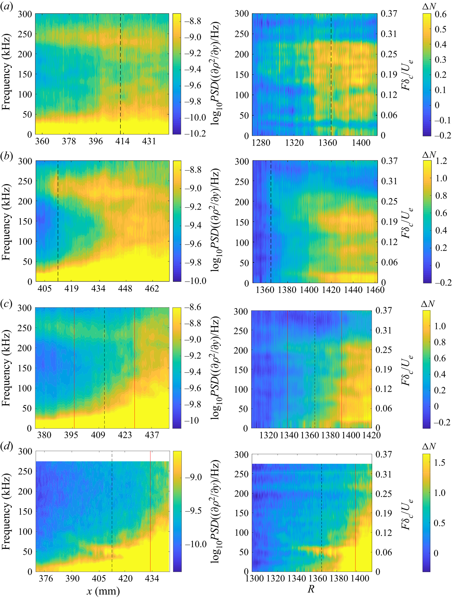
Figure 16. Same as figure 14, but for condition Re45.

For the +10$^\circ$ case, the second-mode disturbances freeze in amplitude within the upstream portion of the separation bubble (third contour of figure 15), but begin to amplify (weakly) within the downstream portion as they approach reattachment, as in the computations of Novikov et al. (Reference Novikov, Egorov and Fedorov2016). Dramatic spectral broadening is observed in the vicinity of reattachment near $X = 430$ mm, or $R = 1390$ (figure 16c). Although it is difficult to discern in the PSD pseudo-streamline spectrum, the $N$-factor spectrum for this test shows evidence of weakly amplifying disturbances at $80$ kHz within the separation bubble from $R=1300\unicode{x2013}1330$, which we have previously shown to correspond to intermittent shear-layer disturbances (Butler & Laurence Reference Butler and Laurence2021a).

In the +15$^\circ$ results we again see a clear shift away from second-mode-dominated behaviour. The bottom-most spatial contour of figure 15 shows amplification of high-frequency content through the entire separation bubble, with the most significant growth again occurring just upstream of reattachment. There also appears to be elevated content along the expected location of the reattachment shock, which was not observed at +10$^\circ$ but is likely related to the previously discussed radiation phenomenon. As in the corresponding Re33 case however, the pseudo-streamline spectra in figure 16(d) (both raw and $N$-factor plots) indicate no significant second-mode peak. Instead, the dominant feature is again the shear-layer instability, which is seen from $X\approx 387$ mm ($R\approx 1320$) and reduces in frequency from approximately $85$ kHz to $50$ kHz at the corner. Substantial low-frequency amplification occurs downstream of the corner near the reattachment zone.

Switching focus to condition Re52, in figure 17 the spatial PSD contours now correspond to $230\unicode{x2013}330$ kHz and the intermittently transitional nature of the incoming boundary layer has a significant effect in all configurations. For the +0$^\circ$ case, this manifests itself as high-frequency content lying significantly above the pseudo-streamline downstream of $X\approx 403$ mm ($R\approx 1450$), where the disturbance strength now peaks. This also corresponds to the location beyond which significant spectral broadening is seen in the pseudo-streamline spectra of figure 18(a). Just downstream of the +5$^\circ$ compression, the high-frequency content amplifies briefly but rapidly before apparently saturating (second contour of figure 17). This is accompanied by nearly instantaneous spectral broadening in figure 18(b), with the power of lower frequencies rising to meet or exceed the second-mode power. The high-frequency content in the +10$^\circ$ case grows steadily along the frustum and decays slightly downstream of separation from $X\approx 403\unicode{x2013}413$ mm in the third contour of figure 17. As the flow reattaches, this content amplifies and spreads out to cover an off-wall distance significantly greater than the upstream boundary-layer thickness, again implying transition. This behaviour is mirrored by the +15$^\circ$ configuration, where the turbulent state of the flare boundary layer is even more obvious. Both separated configurations display effectively instantaneous spectral broadening at the corner in figures 18(c) and 18(d). The low-frequency signature of the shear-layer mode has largely vanished from the streamline spectra for the +15$^\circ$ extension even upstream of thispoint.

Figure 17. Spatial contours of average PSD from $230\unicode{x2013}330$ kHz at condition Re52 for each flare configuration. Separation/reattachment locations are indicated by vertical lines.

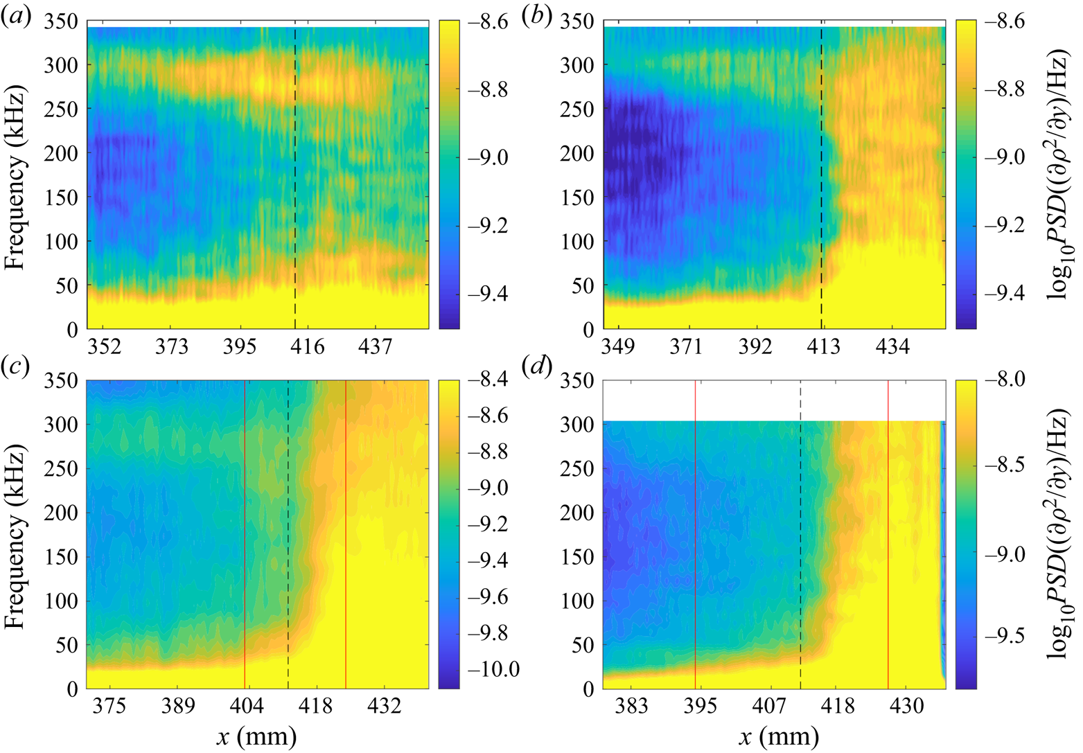
Figure 18. Power spectral densities along pseudo-streamlines at condition Re52 for the (a) +0$^\circ$, (b) +5$^\circ$, (c) +10$^\circ$ and (d) +15$^\circ$ configurations. The dashed and solid vertical lines indicate corner and (where relevant) separation/reattachment locations.

4.2. Low-frequency behaviour

The consistent generation of low-frequency content, particularly in the separated cases, justifies a spatial analysis with the frequency range chosen to bracket the potential shear-layer instability observed thus far in the PCB and schlieren spectra. Figure 19 shows the integrated power within this range, from $40\ {\rm kHz}\text{ to }80\ {\rm kHz}$, for each configuration at condition Re33. Mild growth occurs downstream of the +5$^\circ$ corner in the vicinity of the pseudo-streamline, likely associated with the low-frequency $N$-factor peak shown in figure 14. This is dwarfed however by the growth observed in the separated regions of the +10$^\circ$ and +15$^\circ$ configurations. For the +10$^\circ$ extension, much of the amplification occurs from $X\approx 410\unicode{x2013}430$ mm as the separation bubble is compressing towards reattachment. As mentioned previously, both pseudo-streamline contours (figure 14c) show growth of a distinct $75$ kHz band within this region, whereas the amplification seen along the flare is likely due to the $40$ kHz peak seen in the $N$-factor plot. These observations largely hold for the +15$^\circ$ case, but the disturbance amplification can be discerned as far upstream as $X\approx 390$ mm and reaches a much greater magnitude. There is also evidence of energy emanating away from the shear layer at approximately $X = 415$ mm, which is consistent with the instantaneous behaviour noted in the reference-subtracted sequences.

Figure 19. Spatial contours of average PSD from $40\unicode{x2013}80$ kHz at condition Re33 for each flare configuration. Separation/reattachment locations are indicated by vertical lines.

Figure 20 shows that the +5$^\circ$ compression causes greater low-frequency (now $50\unicode{x2013}90$ kHz) amplification at condition Re45 than at condition Re33. The spatial amplification seen along the flare for this configuration most likely corresponds to the $N$-factor peak at around $80$ kHz in figure 16(b), as both features begin to dissipate at approximately $X = 455$ mm ($R=1430$). The +10$^\circ$ compression again shows evidence of the shear-layer instability developing over the separation bubble, particularly within the downstream portion from $X\approx 415\unicode{x2013}425$ mm; this was obscured in the raw pseudo-streamline spectra (figure 16c), partly because the pseudo-streamline is tuned to the second-mode disturbances and does not follow the maximum amplification of low-frequency structures (which we see in figure 20 occurs instead above the pseudo-streamline). This content amplifies further downstream of reattachment, but the pseudo-streamline spectra suggest this amplification to be caused primarily by spectral broadening and transition. The shear-layer instability for the +15$^\circ$ configuration in the lowermost contour again develops far upstream of the corner. There is a brief but notable drop in PSD directly above the corner at $X = 412$ mm, where significant energy is seen emanating from the shear layer. This drop is not captured in figure 16(d) because the maximum low-frequency fluctuations again occur further from the wall than the pseudo-streamline. The growth and slight decay of the shear disturbances illustrated here correlate well with the production terms for the baroclinic instability identified by Dwivedi et al. (Reference Dwivedi, Sidharth, Nichols, Candler and Jovanović2019) for a two-dimensional compression ramp, suggesting a similar mechanism may be at work. Another particularly strong ray of energy originates from the reattachment zone in the spatial contour, at which point the pseudo-streamline spectrum in figure 16(d) shows significant spectral broadening.

Figure 20. Spatial contours of average PSD from $50\unicode{x2013}90$ kHz at condition Re45 for each flare configuration.

At condition Re52 (not shown), the low-frequency content experiences transition-related amplification in all configurations. The separated cases no longer show significant evidence of the shear-layer instability, though apparently unrelated low-frequency content does amplify within the separation bubbles.

5.1. Attached-flow cases

As has been established, the boundary layer on the straight-cone configuration is largely dominated by the second-mode instability: this is confirmed by the SPOD analysis. The energies of the SPOD modes computed for each condition are given in figure 21, with the highest-ranked mode indicated by a bold line in each case. Throughout this section, only the highest-ranked mode will be considered for analysis, as it represents the greatest energy content and appears to capture the dominant instability mechanisms (in the left plot of figure 21, for example, the second-mode energy near $200$ kHz is much more prominent in the highest-ranked mode than the others). Note that the second-mode peak appears reduced at Re52: this is due to turbulent content which possesses significant flow energy but is less structurally coherent.

Figure 21. The SPOD mode energy for the +0$^\circ$ extension at condition Re33 (left panel), condition Re45 (middle panel) and condition Re52 (right panel).

Eigenvalue contours for select SPOD modes for condition Re33 on the straight cone are given in figure 22. Because they are computed from schlieren images, these eigenvalues correspond to spatially coherent oscillations in the vertical density gradient, $\partial \rho /\partial y$. Note that the colour map for each SPOD mode has been scaled independently to provide the best qualitative visualization of that mode's coherent flow structures (as is the case throughout). The $184$ kHz contours (figure 22b) show the typical rope-like structure of the second-mode disturbances, amplifying from the upstream end of the field of view until dissipating from around $X = 400$ mm. While these second-mode disturbances are dominant, lower-frequency content is also present. Figure 22(a) shows coherent structures at $34$ kHz, with a shallower angle than the second-mode features, amplifying as far upstream as $X = 380$ mm. It is possible that these structures correspond to the first mode, as similar features were observed and speculated to be first-mode waves in Casper et al. (Reference Casper, Beresh, Henfling, Spillers, Pruett and Schneider2016) and Kennedy et al. (Reference Kennedy, Jewell, Paredes and Laurence2022). The large spike in SPOD energy from $250\unicode{x2013}300$ kHz in figure 21 is exemplified by the $280$ kHz mode (figure 22c), which corresponds to uniform flickering; this is thus a noise mode from the schlieren apparatus and can be safely ignored.

Figure 22. The SPOD mode shapes for the +0$^\circ$ configuration at condition Re33 for frequencies of (a) $34$ kHz, (b) $184$ kHz and (c) $281$ kHz.

The enhanced growth of lower-frequency content at condition Re52 is demonstrated by the first three contours of figure 23; such features are also generally representative of the low-frequency content at condition Re45. The $32$ kHz mode (figure 23a) closely resembles the corresponding one at Re33, while the $59$ kHz structures exhibit a similar angle and occupy generally the same region of the boundary layer, suggesting a possible first harmonic. The structures of the $144$ kHz mode (figure 23c), meanwhile, closely resemble those of the dominant second mode but at half the frequency and, thus, may represent a subharmonic. The second-mode structures are now observed at higher frequencies and overpower the flickering noise, with the $294$ kHz mode (figure 23d) demonstrating strong energy even at the upstream edge of the field of view. All modal structures begin to dissipate or lose coherence from $X \approx 430$ mm: this is attributed to the transitional nature of the boundary layer at such high $Re_m$, which degrades the coherency of the flow structures.

Figure 23. The SPOD mode shapes for the +0$^\circ$ configuration at condition Re52 for frequencies of (a) $32$ kHz, (b) $59$ kHz, (c) $144$ kHz and (d) $294$ kHz.

The SPOD energy spectra for the +5$^\circ$ compression (not shown here) still demonstrate distinct peaks surrounding the second-mode fundamental, but with additional regions of lower-frequency elevation. At condition Re33, for instance, the highest-ranked mode contains substantially more energy than the second highest at around $70\unicode{x2013}80$ kHz; this is also the case near $150$ kHz at condition Re45. The mode shapes computed for condition Re33 reveal complex growth of disturbances along the flare, as seen in the contours of figure 24. Some of this growth appears to correspond to modulation of the structures observed in the straight-cone case. For example, the $32$ kHz mode (figure 24a) resembles that seen in figure 22(a), tentatively identified as being generated by first-mode waves. Second-mode content at $199$ kHz (figure 24f) can be seen passing through the corner and intensifying until approximately $X = 450$ mm, matching the saturation point seen in the pseudo-streamline spectrum of figure 14(b). Rope-like structures can also be seen developing just downstream of the corner at $180$ kHz (figure 24e) – the growth of such apparent lower-frequency second-mode disturbances is somewhat surprising given the reduced boundary-layer thickness on the flare. Other lower-frequency structures however do not have a clear analogue in the +0$^\circ$ case. For example, coherent structures at $77$ kHz (figure 24b) appear downstream of the corner and seemingly correspond to a significant $N$-factor peak along the pseudo-streamline (figure 14b). Another mode shape with substantial energy in this region ($125$ kHz) is shown in figure 24(c), though the relevant structures are less clearly periodic than those at the other frequencies shown. As will be discussed in § 6, this growth region correlates well with the appearance of nonlinear interactions, particularly for the $77$ kHz and $125$ kHz structures. An additional mode shape with nonlinear relevance is shown at $161$ kHz (figure 24d); this amplifies downstream of the corner but then loses coherence towards the end of the flare.

Figure 24. The SPOD mode shapes for the +5$^\circ$ configuration at condition Re33 for frequencies of (a) $32$ kHz, (b) $77$ kHz, (c) $125$ kHz, (d) $161$ kHz, (e) $180$ kHz and ( f) $199$ kHz.

Low-frequency content is once more seen to develop downstream of the corner at condition Re45 in figure 25. The $35$ kHz structures again resemble the possible first-mode waves identified in the straight-cone case; the $71$ kHz and $100$ kHz mode shapes (figures 25b and 25c) develop slightly further downstream but share structural similarities with the $35$ kHz mode, and, thus, may represent first and second harmonics. This would reinforce the observation that the attached SWBLI modulates existing disturbances, in this case promoting harmonic development. Particular note should also be taken of the $151$ kHz mode, as this corresponds to a significant $N$-factor peak for the test (figure 16b). As was noted earlier, this elevated $N$ factor may be largely due to the relative weakness of the signal at this frequency upstream (which is reflected by the absence of structures in the SPOD contours); nevertheless, on the flare we see well-defined, coherent structures at this frequency. The SPOD mode shapes within the second-mode band, e.g. at $244$ kHz (figure 25e), show evidence of dissipation due to the onset of turbulence downstream of $X=450$ mm, and energy can be seen radiating away from the boundary layer along the corner shock. High-frequency content is observed at $382$ kHz (figure 25f) from around $X = 420$ mm, likely corresponding to transitional structures.

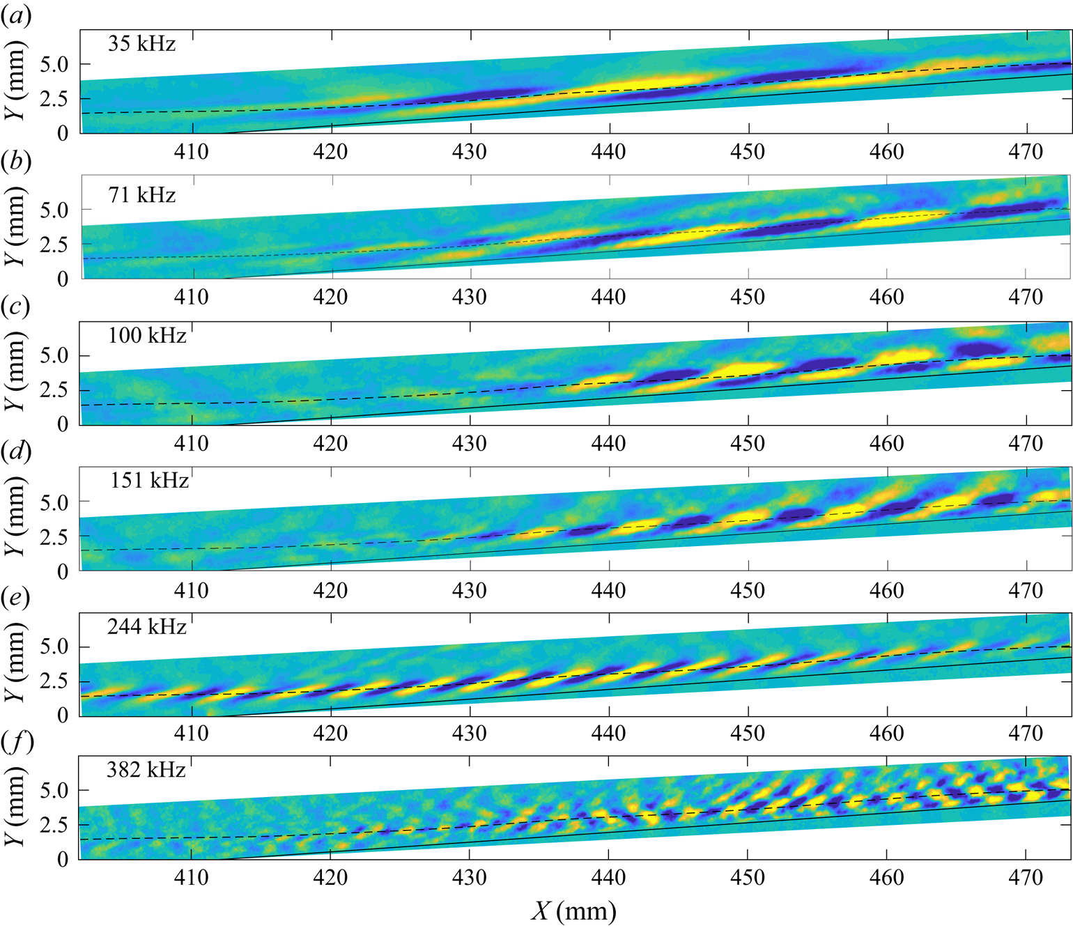
Figure 25. The SPOD mode shapes for the +5$^\circ$ configuration at condition Re45 for frequencies of (a) $35$ kHz, (b) $71$ kHz, (c) $100$ kHz, (d) $151$ kHz, (e) $244$ kHz and ( f) $382$ kHz.

The rapid breakdown induced by the compression corner at condition Re52 is evident in the structure of the SPOD modes shown in figure 26. Low-frequency content appears abruptly at the corner ($61$ kHz and $136$ kHz modes, figures 26a and 26b); these structures have a slightly irregular appearance indicative of contamination by intermittent turbulence. The lack of coherent structures along the frustum at $136$ kHz is somewhat surprising given the spectral peak exhibited by the U3 PCB sensor in figure 7. The higher-frequency mode shapes associated with the second mode generally show a rapid breakdown in structure at the flare, which is to be expected based on the immediate spectral broadening and disappearance of the second-mode peak along the pseudo-streamline. Nevertheless, the $270$ kHz mode, which corresponds closely to the U3 peak second-mode frequency at this condition, persists for a short distance downstream of the corner; this indicates that some wavepackets traverse the SWBLI without immediately breaking down.

Figure 26. The SPOD mode shapes for the +5$^\circ$ configuration at condition Re52 for frequencies of (a) $61$ kHz, (b) $136$ kHz and (c) $270$ kHz.

5.2. Separated-flow cases

A discussion of the major SPOD mode shapes for the +10$^\circ$ extension at the three conditions has been provided in Butler & Laurence (Reference Butler and Laurence2021b). Here we give a brief overview, focusing on those shapes corresponding to frequencies that exhibit significant nonlinear interactions in § 6. Three mode shapes for condition Re33 are shown in figure 27. The second-mode waves at $215$ kHz exhibit the expected rope-like structure, weakening only slightly as they traverse the corner separation, with some evidence of energy passing into the separation bubble. The $42$ kHz mode shape consists of long-wavelength features approximately aligned with the shear layer; these amplify significantly immediately downstream of separation and maintain their amplitude through reattachment. This behaviour is consistent with that of the $40$ kHz $N$-factor peak which develops along the pseudo-streamline (figure 14c). Finally, the mode shape representative of the previously noted shear-layer disturbance at $71$ kHz is shown in figure 27(b). Figure 28 displays two mode shapes for condition Re45. The second-mode structures at $257$ kHz maintain their amplitude downstream of separation, then take on a modified appearance downstream of reattachment. The $61$ kHz mode amplifies within the downstream portion of the separation bubble and appears significantly augmented by the onset of transition downstream of reattachment.

Figure 27. The SPOD mode shapes for the +10$^\circ$ configuration at condition Re33 at (a) $42$ kHz, (b) $71$ kHz and (c) $215$ kHz. Separation and reattachment locations are indicated by the dashed vertical lines.

Figure 28. The SPOD mode shapes for the +10$^\circ$ configuration at condition Re45 at (a) $61$ kHz and (b) $257$ kHz.

As evidenced by the streamline spectra of figures 14(d) and 16(d), the large separation bubble created by the +15$^\circ$ configuration for conditions Re33 and Re45 continues the trend of shifting the dominant modal content to lower frequencies, with significant content under $70$ kHz but little-to-no prominent high-frequency content. This is reflected in the SPOD energy spectra, where the dominant peak at these conditions now corresponds to the shear-layer disturbances at around $40\unicode{x2013}50$ kHz. The highest-rank modes were also elevated slightly around $80\unicode{x2013}90$ kHz, corresponding to the frequency range of the first harmonic of the shear disturbances.

The SPOD mode shapes presented in figure 29 depict the structures of the prominent low-frequency disturbances at condition Re33. The $41$ kHz mode (figure 29b) closely resembles the shear-layer disturbance identified for the +10$^\circ$ configuration (figure 27b) and appears strongest just upstream of reattachment, from $X =420\unicode{x2013}430$ mm. The $58$ kHz mode (figure 29c) develops further upstream within the separation region and radiates energy away from the shear layer. Significant energy is also seen in the $83$ kHz mode (figure 29d) as the separation region compresses, appearing as longitudinal streaks emanating from the boundary layer at $X = 420$ mm. It is notable that this corresponds approximately to the harmonic frequency of the shear-layer disturbances. Very-low-frequency ($14$ kHz) structures aligned with the pseudo-streamline are observed amplifying rapidly in the immediate vicinity of reattachment in figure 29(a). These latter features likely correspond to the lower band of the $N$-factor peak in figure 14(d).

Figure 29. The SPOD mode shapes for the +15$^\circ$ configuration at condition Re33 for frequencies of (a) $14$ kHz, (b) $41$ kHz, (c) $58$ kHz and (d) $83$ kHz. The reattachment location is indicated by the dashed vertical line.

At condition Re45, the +15$^\circ$ configuration is still largely characterized by low-frequency modal structures, which are illustrated by figure 30. The first SPOD contour, computed at $26$ kHz, shows features concentrated around the downstream end of the separation bubble and corresponds approximately to the subharmonic of the shear mode; this will be addressed further in § 6. The mode shape at $52$ kHz (figure 30b) matches the expected structure of the shear-layer disturbance and again amplifies starting directly above the cone/flare junction, while the $60$ kHz mode (figure 30c) shows content developing further upstream with energy radiating away from the shear layer. The angle of these radiating features (which remains approximately constant) is suggestive of frozen Mach radiation, which would indicate that the generating disturbances are moving supersonically with respect to the external flow. To confirm this, in figure 31 we present disturbance propagation speeds computed based on the cross-correlation methodology described by Butler & Laurence (Reference Butler and Laurence2021b). The cross-correlation was performed along a pseudo-streamline now constructed using the maximum intensity of the shear-layer disturbances, with the intensity time-series bandpass filtered from $40$ kHz to $120$ kHz. On this plot we also show the edge velocity, $U_e$, on the straight-cone section, together with the quantity $U_e(1-1/M_e)$, which is the relative sonic line for disturbances. Note that the actual flow velocity above the separated region will be slightly smaller than $U_e$, since the fluid in this region has been processed by the separation shock. In any case, the disturbance speed upstream of the corner ($U_p \approx 620\ {\rm ms}^{-1}$) lies well below the sonic line, indicating that the disturbances here are indeed locally supersonic. Modal content at $103$ kHz (figure 30d) is composed almost entirely of ribbon-like waves emanating from the shear layer ahead of reattachment. The angle of these waves is now close to that of the shear layer itself, suggesting more a subsonic ‘flapping’ motion of the generating disturbances rather than the frozen radiation of the lower-frequency modes. This is consistent with the propagation speed seen in this region in figure 31, which is now much closer to the relative sonic line (also remembering that $U_e$ is a slight overestimate). It is notable that the relevant frequency corresponds closely to the first harmonic of the shear-layer disturbances. The potential nonlinear development of these structures will be studied further in the next section. High-frequency ($223$ kHz) features are observed in figure 30(e) within the severely thinned boundary layer downstream of reattachment.

Figure 30. The SPOD mode shapes for the +15$^\circ$ configuration at condition Re45 for frequencies of (a) $26$ kHz, (b) $52$ kHz, (c) $60$ kHz, (d) $103$ kHz and ( f) $223$ kHz.

Figure 31. Calculated propagation speed of the shear disturbances for the +15$^\circ$ configuration at condition Re45. Here $U_e$ and $M_e$ are the boundary-layer edge velocity and Mach number on the straight cone, and the location of the corner is indicated by the dashed vertical line.

For condition Re52, the mode shapes were generally dominated by turbulent structures, especially on the flare. Second-mode structures were seen upstream of separation, but there was little evidence of shear-layer disturbances.

6.1. Attached-flow cases

We begin by examining the bicoherence spectra observed in the +0$^\circ$ configuration to discern the undisturbed nonlinear behaviour of the wavepackets. Representative bicoherence spectra for condition Re33 are shown in figure 32 for three distinct streamwise stations, annotated with red lines in the top mean flow image. Each of these regions corresponds to 21 pixels along the pseudo-streamline for which the bicoherence spectra have been averaged. The dashed line connecting the vertices [$F_s/4$, $F_s/4$] and [$F_s/2$, 0], where $F_s$ is the sampling frequency, separates the inner triangle (IT) from the outer triangle (OT). The OT (located to the right of this line) is distinct in that it is non-redundant but relies upon aliased information, i.e. for any frequency pair [$f_1$,$f_2$] within the OT, $f_1 + f_2$ will lie above the Nyquist frequency, $F_s/2$. Information within this region thus requires special scrutiny. At the most upstream station, the dominant nonlinear interaction is fundamental resonance at $210$ kHz (i.e. [210,210,420]), as expected based on prior literature. This resonance shifts to lower frequencies downstream to match the fundamental second-mode peak frequency. At the second station, illustrated by the middle contour plot of figure 32, the bicoherence spectrum exhibits elevated levels around [165,30,195]. Such peaks which occur in the vicinity of the second mode and involve low frequencies are typically attributed to sideband interactions, though it is potentially significant that $30$ kHz roughly corresponds to the low-frequency (possibly first-mode) structures observed in the SPOD analysis. The final contour of figure 32 demonstrates that these resonant and sideband interactions persist far along the extension, where the instantaneous images have shown intermittent breakdown of wavepackets.

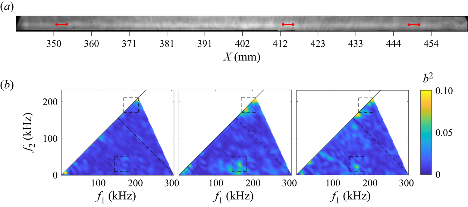
Figure 32. (a) Averaged image for the +0$^\circ$ configuration at condition Re33 with red lines denoting regions for computing the average bicoherence; (b) bicoherence spectra for each region with the contours ordered streamwise from left to right.

We can better visualize the spatial development of these individual interactions as in figure 33, where the r.m.s. bicoherence has been computed within two select regions of the frequency plane (annotated in figure 32 with dashed boxes) for each pixel within the field of view. Figure 33(b) corresponds to fundamental resonance: we see the interaction is generally concentrated around the pseudo-streamline and amplifies along the main cone body. The energy signature of this interaction begins to disperse over the extension as intermittent breakdown occurs, but maintains its presence until the end of the field of view. Note that the downstream part of this contour should be treated with caution, as the resonant peak shifts to frequencies too low to be captured by the considered region far downstream. Figure 33(a) illustrates the spatial distribution of the low-frequency coupling, which appears to be concentrated along the boundary-layer edge; however, it does appear along the pseudo-streamline from $X=415\unicode{x2013}440$ mm, matching the peak intensity of the $34$ kHz SPOD structures in figure 22(a).

Figure 33. Spatial bicoherence contours on the straight cone at condition Re33 for frequency triplets of (a) [165,30,195] and (b) [190,190,380].

The compression-corner configurations generally lead to the development of new nonlinear exchange mechanisms. Figure 34 demonstrates this point for the +5$^\circ$ configuration at condition Re33 (note that the frame rate here has been increased to $822$ kHz, which facilitates better resolution of interactions). The most upstream bispectral plot verifies the presence of fundamental resonance near $200$ kHz as well as low-frequency coupling in the immediate vicinity of the corner. From the spatial contour of figure 35(e), we see that this resonance enters from upstream of the field of view concentrated along the pseudo-streamline and persists downstream of the corner until approximately $X=430$ mm, at which point the interaction dissipates and moves closer to the wall. Indeed, the second streamwise station in figure 34 demonstrates the continued presence of $200$ kHz resonance, but it is absent at the third station.

Figure 34. As in figure 32 but for the +5$^\circ$ configuration at condition Re33.

Figure 35. Spatial bicoherence contours for the +5$^\circ$ flare at condition Re33 for frequency triplets of (a) [75,75,150], (b) [160,10,170], (c) [160,70,230], (d) [120,120,240] and (e) [200,200,400].

Multiple additional resonant interactions develop at the second station of figure 34 around frequencies of 70–80 kHz and 150–160 kHz. In addition to the interaction between these two frequency bands ([160,70,230]), there is a large degree of low-frequency coupling in the vicinity of [160,10,170]. As seen in figures 35(a)–35(c), these interactions peak sharply from $X=420\unicode{x2013}430$ mm. This region corresponds closely to where the $77$ kHz and $161$ kHz SPOD mode shapes presented in figure 24 first develop, with the $161$ kHz structure appearing slightly further upstream. The interaction at [160,70,230] can thus best be explained as deconstructive interference between second-mode wavepackets at $230$ kHz and the low-frequency content to produce additional low-frequency structures. Notably, the interaction at [160,10,130] exhibits substantial energy from just upstream of the corner and above the pseudo-streamline; this part of the contour likely corresponds to the corner shock, as mean flow interactions are captured by this bi-frequency region. The resonant interaction at $120$ kHz that peaks at the third station in figure 34 has the same general spatial distribution (figure 35d) as the preceding interactions, but shifted downstream. This interaction can be linked to the SPOD structure at $125$ kHz (figure 24c), which peaks in amplitude near $X=440$ mm and shows a broadly similar distribution of energy.

Spatial bicoherence distributions for several of the notable interactions on the +5$^\circ$ flare at condition Re45 are given in figure 36. The first three contours correspond to resonant interactions at $35$ kHz, $70$ kHz and $230$ kHz. The dominant feature for all these interactions is a band of substantially elevated signals lying well above the pseudo-streamline on the flare. This band originates from 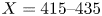$X=415\unicode{x2013}435$ mm depending on the frequency and much of this content, especially downstream, likely corresponds to turbulent features. Nevertheless, we can deduce other regions of nonlinear significance in these contours. Resonance of the second-mode fundamental at $230$ kHz (figure 36c) is seen along the pseudo-streamline at the beginning of the field of view but rapidly drops off downstream of the corner. The $70$ kHz resonance develops slightly upstream of the corner and is also clearly concentrated along the pseudo-streamline until approximately $420$ mm. Both the $35$ kHz resonance and the [135,10,145] interaction (figure 36d) spike in amplitude dramatically from $410\unicode{x2013}420$ mm, with much of the signal concentrated above the pseudo-streamline; this behaviour of the low-frequency resonance is consistent with the emergence of the SPOD mode in figure 25(b). The energy concentration of the [135,10,145] contour correlates with a locally well-defined SPOD structure at $140$ kHz not shown in the preceding discussion and likely corresponds to a mean flow interaction with the corner shock. Synthesizing the results from both conditions, the +5$^\circ$ compression causes a localized spike in nonlinear interactions early on the flare, which may facilitate energy transfer and alter the transition process significantly.

Figure 36. Spatial bicoherence contours for the +5$^\circ$ flare at condition Re45 for frequency triplets of (a) [35,35,70], (b) [70,70,140], (c) [230,230,460] and (d) [135,10,145].

6.2. Separated-flow cases

There was a general decrease in nonlinear interactions for the +10$^\circ$ configuration compared with the +5$^\circ$ configuration at condition Re33; figure 37 shows the spatial distribution of three of the more prominent interactions. Fundamental resonance at [220,220,440] and low-frequency coupling of the second-mode waves at [220,20,240] are captured upstream of the separation point but quickly die off within the separated region, where there is generally little evidence of high-frequency interactions. A new, low-frequency resonant interaction at [45,45,90] appears downstream of separation however, and may correspond to the SPOD mode shape in figure 27(a).

Figure 37. Spatial bicoherence contours for the +10$^\circ$ flare at condition Re33 for frequency triplets of (a) [45,45,90], (b) [220,20,240] and (c) [220,220,440].

There is a significant increase in nonlinearity within the separation region and in the vicinity of reattachment at condition Re45, and several representative bispectral plots are presented in figure 38. At the first station, located within the shear layer just downstream of the corner, there now exist two distinct resonant interactions at approximately $70$ kHz and $140$ kHz. We also note prevalent high-frequency interactions in the vicinity of [320,10,330] and [320,180,500]; these latter interactions may correspond to harmonic content aliased down from $500$ kHz. Just upstream of reattachment, in the middle contour of figure 38, the low-frequency resonance shifts down to $55$ kHz while the $140$ kHz resonance continues to amplify. Figure 39(a) shows that the low-frequency resonance peaks within a confined spatial region along the pseudo-streamline, which generally matches the behaviour of the $61$ kHz SPOD mode in figure 28(a). The $75$ kHz resonance depicted in figure 39(b) corresponds to essentially the same phenomenon but appearing slightly further upstream and shifted in frequency. As with the +5$^\circ$ configuration, the streamline curvature appears to create a concentrated region close to the corner in which the nonlinear interactions are greatly enhanced. The $160$ kHz resonant interaction, although prominent in the two downstream stations of figure 38, demonstrates little spatial coherence in figure 39(c) and seems to be largely due to contamination from intermittent turbulence. This is the case for many of the interactions which appear in the third station of figure 38, just downstream of reattachment.

Figure 38. As in figure 32 but for the +10$^\circ$ flare at condition Re45.

Figure 39. Spatial bicoherence contours for the +10$^\circ$ flare at condition Re45 for frequency triplets of (a): [55,55,110], (b) [75,75,150] and (c) [160,160,320].

The reduced frame rates employed with the +15$^\circ$ configuration ($440$ kHz at condition Re33 and $550$ kHz at Re45) render it impossible to properly resolve nonlinear interactions involving second-mode disturbances without significant aliasing. Fortunately, the preceding sections have demonstrated that the unsteady flow field in this configuration is largely dominated by lower-frequency structures which lie well below the Nyquist limit. At condition Re33, as with the +10$^\circ$ configuration, there are no discernible peaks in the bicoherence throughout much of the upstream portion of the separation bubble. The first region presented in figure 40 is located upstream of the corner near where the shear-layer disturbances are first observed in instantaneous images: here, the bicoherence spectrum shows resonance at $53$ kHz, corresponding to the dominant frequency of the shear waves. At the second station, downstream of the corner, this resonance has amplified substantially (though this is not immediately clear from the figure, since the colour scale has saturated) and shifted to $40$ kHz, consistent with the decrease in frequency seen along the pseudo-streamline. The spatial contour of figure 41(a) shows this interaction is concentrated both near and above the pseudo-streamline from $X=418\unicode{x2013}425$ mm as the boundary layer recompresses, which is also where the $83$ kHz SPOD mode in figure 29(d) becomes prominent; this is consistent with the latter corresponding to a harmonic of the shear-layer disturbance.

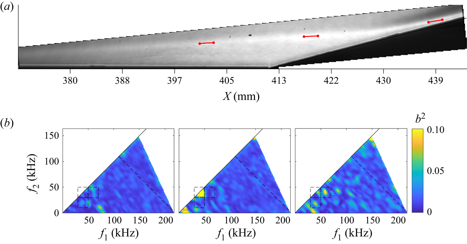
Figure 40. As in figure 32 but for the +15$^\circ$ configuration at condition Re33.

Figure 41. Spatial bicoherence contours for the +15$^\circ$ flare at condition Re33 for frequency triplets of (a) [40,40,80], (b) [40,20,60] and (c) [60,40,100].

Downstream of reattachment (third station of figure 40), a series of interactions can be seen to lie approximately along vertical and horizontal lines corresponding to $f_1 = 40$ kHz and $f_2 = 40$ kHz; we note also that these peaks have approximately uniform spacing of $\Delta f = 20$ kHz. Interaction peaks at [42,20,62] and [60,40,100] are presented in figures 41(b) and 41(c). Both of these contours are concentrated within a similar region of the flow field as the main energy in the $14$ kHz SPOD mode in figure 29(a). As with the $40$ kHz resonance, these interactions peak in strength as the boundary layer reattaches, but exhibit significant intensity far upstream of this. All of this suggests that the shear disturbances couple with other lower-frequency content to facilitate energy transfer within the shear layer. This also demonstrates the shortcomings of the pseudo-streamline for this analysis however, as these interactions follow very different trajectories.

At condition Re45, resonance of the shear-layer instability at [50,50,100] is observed in the first probed region of figure 42 as far upstream as $X=405$ mm. This interaction amplifies downstream at the second station (just upstream of reattachment), while new resonances appear at $25$ kHz and $95$ kHz: these interactions are notable in that they correspond approximately to the subharmonic and harmonic of the shear-layer disturbances, respectively. The spatial distribution of the fundamental shear-mode resonance ([50,50,100]) is shown in figure 43(b) to attain significant energy by $X\approx 410$ mm and then peak just above the pseudo-streamline as the boundary layer recompresses, just as it did at condition Re33. Now, however, the bicoherence peak is no longer confined close to the boundary of the separation bubble, with a ray of elevated signal extending upwards from the shear layer. The bicoherence peak and this ray of elevated signal align well with the SPOD structure displayed in figure 30(d) at $103$ kHz, suggesting that the ribbon-like waves of energy which emanate from the shear layer may be caused by nonlinear resonance of the shear waves as they approach reattachment. The potential subharmonic resonance at $25$ kHz is illustrated by the contour of figure 43(a) and peaks both above and below the pseudo-streamline within the same region as the fundamental shear-mode resonance. This interaction immediately precedes the development of the $26$ kHz structures resolved by the SPOD analysis in figure 30(a). Another interesting feature of the bicoherence spectrum at the second station is the peak which develops at [100,50,150], potentially corresponding to an interaction between the shear-layer disturbance and its first harmonic. The spatial distribution of this interaction (figure 43c) again appears as a ray emanating from $X=418$ mm and closely aligns with the $103$ kHz SPOD mode shape in figure 30(d), providing evidence that higher-harmonic content is generated within the region of streamline curvature as the shear layer approaches the flare.

Figure 42. (a,b) Averaged image for the +15$^\circ$ configuration at condition Re45 with red lines denoting regions for computing the bicoherence; (c,d) bicoherence spectra for each region with the contours ordered streamwise from top left to bottom right.

Figure 43. Spatial bicoherence contours for the +15$^\circ$ flare at condition Re45 for frequency triplets of (a) [25,25,50], (b) [50,50,100], (c) [100,50,150] and (d) [215,20,235].

Within the vicinity of reattachment (probed by the third station in figure 42), interactions develop along the band corresponding roughly to $f_2 = 20$ kHz. This band of interactions persists and strengthens downstream at the final station (note the increased contour limits there). These interactions are likely facilitated by low-frequency structures similar to the $26$ kHz SPOD mode (figure 30a), which are concentrated near reattachment. Notably, these downstream interactions also involve some much higher frequencies. Figure 43(d) shows that the interaction [215,20,235] is concentrated entirely within the compressed boundary layer downstream of reattachment, correlating well with the high-frequency structures resolved along the flare by the SPOD analysis, for example, in figure 30( f).