


1. Introduction
Internal waves generated by tides and winds can cause intense mixing in the deep ocean (Alford Reference Alford2003; Garrett Reference Garrett2003). Dissipation of these internal waves plays a crucial role in meridional overturning circulation (Munk & Wunsch Reference Munk and Wunsch1998) and processes such as nutrient and plankton transport (Garrett & Munk Reference Garrett and Munk1979).
Triadic resonance is one of the important mechanisms leading to internal wave dissipation (Staquet & Sommeria Reference Staquet and Sommeria2002). A well-studied manifestation of triadic resonance is parametric subharmonic instability (PSI), where a primary internal wave of frequency  $\omega$ and wave vector $\boldsymbol {k}$ is unstable to perturbations of two secondary waves with frequencies $\omega _{1,2} = \omega /2$ and wave vectors $\boldsymbol {k}_{\boldsymbol {1}}$ and $\boldsymbol {k}_{\boldsymbol {2}}$ such that $\boldsymbol {k}_{\boldsymbol {1}} + \boldsymbol {k}_{\boldsymbol {2}} = \boldsymbol {k}$. (Hasselmann Reference Hasselmann1967; Koudella & Staquet Reference Koudella and Staquet2006). Field observations (Alford et al. Reference Alford, MacKinnon, Zhao, Pinkel, Klymak and Peacock2007; MacKinnon et al. Reference MacKinnon, Alford, Sun, Pinkel, Zhao and Klymak2013), however, show much less energy transfer from internal tides to subharmonic waves than what is predicted by the theory of PSI. The effects of various realistic ocean settings such as non-uniform stratification (Young, Tsang & Balmforth Reference Young, Tsang and Balmforth2008; Gayen & Sarkar Reference Gayen and Sarkar2013; Gururaj & Guha Reference Gururaj and Guha2020), finite width of the wave beam (Bourget et al. Reference Bourget, Scolan, Dauxois, Le Bars, Odier and Joubaud2014; Dauxois et al. Reference Dauxois, Joubaud, Odier and Venaille2018) and background flow (Fan & Akylas 2019, 2021) are potential reasons for the discrepancy between theory and observations of PSI. The effects of a background flow is the focus of the current study, albeit on a different manifestation of triadic resonance as described below.
Another manifestation of triadic resonance occurs when two monochromatic (frequency  $\omega$) primary internal waves resonantly excite a secondary wave at superharmonic frequency $2\omega$. Resonant generation of superharmonic internal waves has been studied in the context of interacting internal wave beams (Teoh, Ivey & Imberger Reference Teoh, Ivey and Imberger1997; Tabaei, Akylas & Lamb Reference Tabaei, Akylas and Lamb2005; Jiang & Marcus Reference Jiang and Marcus2009). Tide–topography interaction (Lamb Reference Lamb2004; Korobov & Lamb Reference Korobov and Lamb2008), internal wave beam reflection from a solid boundary (Javam, Imberger & Armfield Reference Javam, Imberger and Armfield1999; Peacock & Tabaei Reference Peacock and Tabaei2005; Gerkema, Staquet & Bouruet-Aubertot Reference Gerkema, Staquet and Bouruet-Aubertot2006; Rodenborn et al. Reference Rodenborn, Kiefer, Zhang and Swinney2011) or a pycnocline (Thorpe Reference Thorpe1998; Gayen & Sarkar Reference Gayen and Sarkar2013; Diamessis et al. Reference Diamessis, Wunsch, Delwiche and Richter2014; Wunsch et al. Reference Wunsch, Ku, Delwiche and Awadallah2014; Mercier et al. Reference Mercier, Mathur, Gostiaux, Gerkema, Magalhães, Da Silva and Dauxois2015) are example scenarios where interacting internal wave beams generate superharmonic internal waves. Higher harmonic generation due to surface reflection of internal tides has been observed in the ocean too (Xie et al. Reference Xie, Shang, van Haren and Chen2013). In a fixed-depth domain like the region between the ocean floor and surface, only discretized wavenumbers are possible and linear internal wave fields are a superposition of internal wave modes. Superharmonic generation due to modal interactions, as summarized below, has received much attention recently.
In a uniform stratification with no shear, interaction between two different internal wave modes  $m$ and $n$ at a given frequency $\omega$ can resonantly excite a superharmonic $2\omega$ internal wave mode $|m-n|$ at specific values of $\omega$ if $m/3< n<3m$ (Thorpe Reference Thorpe1966). As shown in figure 1, only a fraction of the points where the horizontal resonance condition is satisfied are actual triadic resonance locations. The amplitude evolution of such resonant triads in a uniform stratification with no shear has recently been studied numerically (Varma, Chalamalla & Mathur Reference Varma, Chalamalla and Mathur2020) and experimentally (Husseini et al. Reference Husseini, Varma, Dauxois, Joubaud, Odier and Mathur2020). In contrast to a uniform stratification, several more triadic resonances occur in a finite-depth non-uniform stratification (Varma & Mathur Reference Varma and Mathur2017), including the possibility of self-interacting individual modes exciting superharmonic wave fields (Thorpe Reference Thorpe1968; Sutherland Reference Sutherland2016; Wunsch Reference Wunsch2017). Varma et al. (Reference Varma, Chalamalla and Mathur2020) and Baker & Sutherland (Reference Baker and Sutherland2020) have studied amplitude evolution in self-interacting modes at and off resonance, respectively.

Figure 1. (a) Dispersion curves ( $\omega$ vs $k_q$, grey lines) for mode numbers $q = 1,2,3,4,5$ in a uniform stratification with no shear. The black lines show $2\omega$ vs $k_m+k_n$ for $m+n = 2$ to $10$, with modes $m$ and $n$ being at frequency $\omega$. Horizontal resonance condition $k_m+k_n = k_q$ is satisfied at the points of intersection (filled and unfilled circles). Filled circles represent actual resonances. (b) Number ( $N_H$, unfilled circles) of modal interactions (between modes $m$ and $n$ at frequency $\omega$, $0<\omega <0.5$) for which the horizontal resonance condition $k_m + k_n = k_q$ (mode $q$ being at $2\omega$) is satisfied, plotted as a function of $m+n$. Number $N_R$ (filled circles) from the $N_H$ modal interactions that are also resonances. The symbol $\lfloor \ \rfloor$ refers to the floor operator.
In an inviscid, stratified shear flow, if the gradient Richardson number is greater than  $1/4$ throughout the domain, Booker & Bretherton (Reference Booker and Bretherton1967) showed that significant momentum is transferred from internal waves to the mean flow at the critical layer (where internal wave phase velocity matches the local background horizontal velocity), and strong nonlinear effects ensue. As a result, numerous studies have considered nonlinear resonant interactions near the critical layer (Brown & Stewartson Reference Brown and Stewartson1980; Grimshaw Reference Grimshaw1988, Reference Grimshaw1994) in infinite-depth media. To complement the studies of Brown & Stewartson (Reference Brown and Stewartson1980, 1982a,b), Grimshaw (Reference Grimshaw1988, Reference Grimshaw1994) derived amplitude evolution equations for primary (i.e. three interacting first-order waves) and secondary (i.e. a second-order wave interacting with two first-order waves) interactions, respectively, in a slowly varying background shear and stratification in infinite depth. While Grimshaw (Reference Grimshaw1988) focused on ‘weak resonance’ (resonance conditions satisfied only on certain surfaces in space and time) near the critical layer, he pointed out that triadic resonance in the homogeneous flow represents the leading-order ‘strong resonance’ conditions in weakly inhomogeneous flow. In the specific case of stratified, anti-symmetric shear layer, Kelly (Reference Kelly1968) analysed the second-order resonant interactions of two specific interacting singular neutral modes at constant frequency and numerically showed how the amplitude of different waves is modulated. In a finite-depth stratified shear flow, the necessary condition for an explosive interaction (i.e. finite time blow-up in the amplitude evolution) of internal wave modes is the existence of a critical layer (Becker & Grimshaw Reference Becker and Grimshaw1993; Vanneste & Vial Reference Vanneste and Vial1994). Considering a sinusoidal background velocity profile in a uniform stratification and fixed horizontal wavenumbers $(k_1, k_2, k_3)$ that satisfy the triadic resonance condition $k_1 + k_2 + k_3 = 0$, Vanneste & Vial (Reference Vanneste and Vial1994) numerically showed how different interaction coefficients vary with wave amplitudes, and thereby lead to resonance.
Realistic ocean settings include factors such as non-uniform stratification, background rotation, background shear, finite depth, excitation of a wide range of wavenumbers etc. An earlier study (Varma & Mathur Reference Varma and Mathur2017) has shown modal interactions, including self-interaction, can lead to resonant generation of superharmonic internal waves in a finite-depth ocean-like non-uniform stratification with background rotation. Here, we consider the effects of inhomogeneity introduced by a background flow, thus building towards a generalization of the effects of inhomogeneities on finite-depth internal wave triadic resonances. Specifically, we consider triadic resonances in a finite-depth uniform stratification in the presence of an ocean-like nonlinear background shear flow (corresponding to the wind drift layer) that monotonically increases from zero at the ocean floor to a finite value at the ocean surface. With no critical layers being present for discrete modes in a continuous shear flow (Banks, Drazin & Zaturska Reference Banks, Drazin and Zaturska1976), and motivated by forcing mechanisms being at specific frequencies in the ocean (the semi-diurnal frequency, for example), we consider triadic resonances resulting from interaction between two discrete modes at the same frequency. An analytical treatment of the weak shear limit is presented, providing insights into why inhomogeneity significantly increases the number of possible resonances. A systematic study on the effects of Richardson number, spanning weak to strong shear limits, on the occurrence of triadic resonances is then performed. Owing to the loss of symmetry about the  $\omega = 0$ axis in the dispersion curves when background flow is present, both cograde (modes that travel faster than the maximum background flow velocity) and retrograde (modes that travel slower than the minimum background flow velocity) modes are considered.
The governing equations, and weakly nonlinear solutions resulting from modal interactions, are presented in § 2.1. An analytical treatment of the weak shear limit in given in § 2.2. Section 3 discusses the results and compares the solutions from asymptotics and numerics. In § 3, a systematic study of the effects of Richardson number, including weak and strong shear limits, is presented. A brief discussion and a summary of our conclusions are provided in § 4.
2. Theory
2.1. Governing equations
We consider an inviscid, two-dimensional flow in a uniformly stratified fluid of depth  $H$ in the Boussinesq approximation. The base flow state is described by a stably stratified, linear density profile $\bar {\rho }(z)$ and a vertically varying steady horizontal shear flow $U(z)\boldsymbol {e}_x$. The corresponding constant Brunt–Väisälä frequency is $N = \sqrt {-(g/\rho ^{*})(\textrm {d}\bar {\rho }/\textrm {d}z)}$, where $\boldsymbol {g} = -g\boldsymbol {e}_z$ is gravitational acceleration and $\rho ^{*}$ a reference density. The non-dimensional governing equations for the perturbation flow field are (Tsutahara Reference Tsutahara1984)
 \begin{align} &\left(\frac{\partial}{\partial t}+ U \frac{\partial}{\partial x}\right)^{2}\nabla^{2} \psi - \frac{\textrm{d}^{2} U}{\textrm{d} z^{2}}\left(\frac{\partial}{\partial t}+ U \frac{\partial}{\partial x}\right)\frac{\partial \psi}{\partial x} + \frac{\partial^{2} \psi}{\partial x^{2}} \nonumber\\ &\quad ={-}\left(\frac{\partial}{\partial t}+ U \frac{\partial}{\partial x}\right)J(\psi,\nabla^{2} \psi) - \frac{\partial}{\partial x}J(\psi, b), \end{align}
 \begin{align} &\left(\frac{\partial}{\partial t} + U \frac{\partial }{\partial x}\right)b + \frac{\partial \psi}{\partial x} ={-} J(\psi, b). \end{align}
All quantities (including  $U$) in (2.1) and (2.2) are non-dimensional, using $H$,
$H$,  $1/N$ and $\rho ^{*}$ as the length, time and density scales, respectively. Here, $t$,
$t$,  $x$ and $z$ are time, horizontal and vertical coordinates, respectively and the Jacobian is defined as $J(A,B) = (\partial A/\partial x)(\partial B/\partial z) - (\partial A/\partial z)(\partial B/\partial x)$. The non-dimensional perturbation flow field is described by $(u,w) = (-\partial \psi /\partial z, \partial \psi /\partial x)$, where $\psi (x,z,t)$ is the perturbation stream function. The buoyancy perturbation is $b = -g\rho /(N^{2} H)$, where $\rho (x,z,t)$ is the non-dimensional perturbation density. The no-penetration boundary condition is given by $w(x,z=0,t) = w(x,z=1,t) = 0$, with $z = 0$ and $z = 1$ denoting the ocean bottom and top (rigid lid), respectively.
Assuming a regular perturbation expansion in  $\epsilon$, a small parameter that quantifies the relative magnitude of the nonlinear terms in the governing equations, we seek solutions for the perturbation wave field in the following form:
 \begin{equation} (\psi, b) = \epsilon (\psi_1, b_1) + \epsilon^{2} (\psi_2, b_2) + \cdots. \end{equation}
The  $O(\epsilon )$ wave field $(\psi _1, b_1)$, governed by linear internal wave equations, is assumed to comprise a superposition of several modes at a frequency $\omega$
 \begin{equation} \left.\begin{gathered} \psi_1 = \sum_{j={-}\infty}^{\infty}\frac{1}{2}A_j\phi_j(z) \exp({\textrm{i} k_j (x - c_j t)}) + \textrm{c.c.}, \\ b_1 = \sum_{j={-}\infty}^{\infty}\frac{1}{2}A_j\frac{\phi_j(z)}{(c_j - U)} \exp({\textrm{i} k_j (x - c_j t)}) + \textrm{c.c.}, \end{gathered}\right\}\end{equation}
where  $A_j$, $k_j$ and $c_j(=\omega /k_j)$ are the complex amplitude, horizontal wavenumber and phase velocity, respectively of mode $j$, with c.c. denoting complex conjugate. The vertical mode shape, $\phi _j(z)$ is governed by the Taylor–Goldstein–Haurwitz equation (Kundu & Cohen Reference Kundu and Cohen2001)
 \begin{equation} \left[(U-c_j)^{2}\left(\frac{\textrm{d}^{2}}{\textrm{d}z^{2}} - k_j^{2}\right) + 1 - (U-c_j)\frac{\textrm{d}^{2}U}{\textrm{d}z^{2}}\right]\phi_j(z) = 0,\end{equation}
along with the no-penetration boundary conditions given by  $\phi _j(z=0) = \phi _j(z=1) = 0$. The wave field in (2.4) could represent a linear wave field generated by forcing at a specific frequency, internal tides generated by barotropic forcing on topography (Garrett & Kunze Reference Garrett and Kunze2007) for example.
At  $O(\epsilon ^{2})$, the governing equations (2.1)–(2.2) give
 \begin{align} &\left(\frac{\partial}{\partial t}+ U \frac{\partial}{\partial x}\right)^{2}\nabla^{2} \psi_2 - \frac{\textrm{d}^{2} U}{\textrm{d} z^{2}}\left(\frac{\partial}{\partial t} + U \frac{\partial}{\partial x}\right)\frac{\partial \psi_2}{\partial x} + \frac{\partial^{2} \psi_2}{\partial x^{2}} \nonumber\\ &\quad ={-}\left(\frac{\partial}{\partial t}+ U \frac{\partial}{\partial x}\right)J(\psi_1,\nabla^{2} \psi_1) - \frac{\partial}{\partial x}J(\psi_1, b_1), \end{align}
 \begin{align} &\left(\frac{\partial}{\partial t} + U \frac{\partial }{\partial x}\right)b_2 + \frac{\partial \psi_2}{\partial x} ={-} J(\psi_1, b_1). \end{align}
Substituting  $(\psi _1,b_1)$ from (2.4) in (2.6), the right-hand side of (2.6) can be written as
 \begin{gather} \sum_{m={-}\infty}^{\infty}\sum_{n={-}\infty}^{\infty}\left[\left(\tfrac{1}{4}P_{mn}(z)\exp({\textrm{i}(\theta_m+\theta_n)}) + \textrm{c.c.}\right) + \left(\tfrac{1}{4}Q_{mn}(z)\exp({\textrm{i}(\theta_m-\theta_n)}) + \textrm{c.c.}\right)\right],\end{gather}
 \begin{gather} P_{mn}(z) =A_mA_n\left(k_m+k_n\right)\left[\left(U-C_{mn}\right)\left(k_m\phi_m\frac{\textrm{d}}{\textrm{d}z} - k_n\frac{\textrm{d}\phi_m}{\textrm{d}z}\right)\left(\frac{\textrm{d}^{2}}{\textrm{d}z^{2}} - k_n^{2}\right)\phi_n \right. \nonumber\\ \hspace{-2.2pc} \left.- \left(\frac{k_n\phi_n}{(c_n - U)}\frac{\textrm{d}\phi_m}{\textrm{d}z} - \phi_m k_m \frac{\textrm{d}}{\textrm{d}z}\left(\frac{\phi_n}{(c_n - U)}\right)\right)\right], \end{gather}
 \begin{gather} Q_{mn}(z)=A_mA_n^{*}\left(k_m-k_n\right)\left[U\left(k_m\phi_m\frac{\textrm{d}}{\textrm{d}z} + k_n\frac{\textrm{d}\phi_m}{\textrm{d}z}\right)\left(\frac{\textrm{d}^{2}}{\textrm{d}z^{2}} - k_n^{2}\right)\phi_n\right.\nonumber\\\hspace{1.5pc} \left.+ \left(\frac{k_n\phi_n}{(c_n - U)}\frac{\textrm{d}\phi_m}{\textrm{d}z} + \phi_m k_m \frac{\textrm{d}}{\textrm{d}z}\left(\frac{\phi_n}{(c_n - U)}\right)\right)\right], \end{gather}
thus comprising superharmonic (frequency  $2\omega$) and time-independent mean-flow terms. Here, $\theta _j = k_j(x - c_j t)$, $C_{mn} = 2\omega /(k_m+k_n)$ and $A_n^{*}$ is the complex conjugate of amplitude $A_n$. The particular solution of (2.6) can now be sought in the form
 \begin{align} \psi_2 &= \sum_{m={-}\infty}^{\infty}\sum_{n={-}\infty}^{\infty}\left[\left(\tfrac{1}{2}h_{mn}(z)\exp({\textrm{i}(\theta_m+\theta_n)}) + \textrm{c.c.}\right) \right.\nonumber\\ &\quad \left.+ \left(\tfrac{1}{2}g_{mn}(z)\exp({\textrm{i}(\theta_m-\theta_n)}) + \textrm{c.c.}\right)\right], \end{align}
where  $h_{mn}(z)$ and $g_{mn}(z)$ are vertical structures of the superharmonic and mean-flow terms, respectively, resulting from the interaction between modes $m$ and $n$. They satisfy the following equations, obtained from (2.6):
 $$\begin{gather} \left[(U-C_{mn})^{2}\left(\frac{\textrm{d}^{2}}{\textrm{d}z^{2}} - (k_m+k_n)^{2}\right) + 1 - (U-C_{mn})\frac{\textrm{d}^{2}U}{\textrm{d}z^{2}}\right]\bar{h}_{mn}(z) = \frac{-\left(P_{mn}+P_{nm}\right)}{2(k_m+k_n)^{2}}, \end{gather}$$
 $$\begin{gather}\left[U^{2}\left(\frac{\textrm{d}^{2}}{\textrm{d}z^{2}} - (k_m-k_n)^{2}\right) + 1 - U\frac{\textrm{d}^{2}U}{\textrm{d}z^{2}}\right]\bar{g}_{mn}(z) = \frac{-\left(Q_{mn}+Q_{nm}\right)}{2(k_m-k_n)^{2}}, \end{gather}$$
where  $\overline {h}_{mn}(z) = h_{mn}(z) + h_{nm}(z)$ and $\bar {g}_{mn}(z) = g_{mn}(z) + g_{nm}(z)$. The no-penetration boundary conditions are: $\bar {h}_{mn}(z = 0)=\bar {h}_{mn}(z = 1)=\bar {g}_{mn}(z = 0)=\bar {g}_{mn}(z = 1)= 0$. The magnitude of the mean-flow term in (2.11) could potentially be influenced by a class of resonances considered by Phillips (Reference Phillips1968), who studied the interaction between an upward and a downward propagating plane internal wave in the presence of a steady (zero frequency) shear flow with twice the vertical wavenumber of the plane waves. The focus of the current study, however, is the superharmonic part of the $O(\epsilon ^{2})$ wave field, to specifically identify the role of the background shear flow $U(z)$. Before proceeding with a fully numerical solution of (2.12), it is instructive to analyse the asymptotic limit of weak shear.
2.2. Weak shear limit
To perform an asymptotic analysis in the weak shear limit, we define a small parameter  $\delta = \xi /\sqrt {Ri}$, where $Ri = N^{2}L_s^{2}/U_s^{2}$ is the Richardson number and $\xi = L_s/H$ is the ratio of shear flow length scale to the ocean depth; $U_s$ and $L_s$ are dimensional velocity and length scales of the background shear flow. In the weak shear limit ( $\delta \ll 1$), we write
 \begin{equation} U(z) = \delta\upsilon(z), \end{equation}
where  $\upsilon (z)$ is an $O(1)$ function describing the vertical structure of $U(z)$ (recall that $U(z)$ is non-dimensional, with $NH$ being the velocity scale used for the non-dimensionalization). We will make the reasonable assumption of $L_s/H < 1$. This implies, in conjunction with $\delta \ll 1$, that the shear flow time scale $L_s/U_s$ is much larger than the stratification time scale $1/N$ ( $Ri\gg 1$, in other words). We proceed to analytically solve the $O(\epsilon )$ and $O(\epsilon ^{2})$ equations presented in § 2.1, up to $O(\delta ^{1})$, with the assumption that $\delta ^{2}\ll \epsilon \ll \delta$.
2.2.1. The  $O(\epsilon )$ equation

We begin by seeking a regular perturbation series (in  $\delta$) solutions for the vertical mode shapes (2.5) upon substituting $U(z) = \delta \upsilon (z)$. For a fixed frequency $\omega$, we write
 \begin{equation} (\phi_j, k_j) = (\phi_{j,0}, k_{j,0}) + \delta (\phi_{j,1}, k_{j,1}) + \delta^{2} (\phi_{j,2}, k_{j,2}) + \cdots, \end{equation}
where  $\phi _j$ and $k_j$ are the mode shape and horizontal wavenumber of mode $j$, respectively. At $O(\delta ^{0})$, (2.5) reduces to the linear internal wave equation in quiescent fluid
 \begin{equation} \mathcal{L}_j\phi_{j,0}(z) = 0,\end{equation}
where,  $\mathcal {L}_j = (\textrm {d}^{2}/\textrm {d}z^{2}+k_{j,0}^{2}(1-\omega ^{2})/\omega ^{2})$, and the boundary conditions are $\phi _{j,0}(z=0) = \phi _{j,0}(z=1) = 0$. The solutions of (2.16) are given by $\phi _{j,0}(z) = \sin (j{\rm \pi} z)$, $k_{j,0} = j{\rm \pi} \omega /\sqrt {1-\omega ^{2}}$, with $j$ being the mode number. In this subsection, we assume $\omega <1$, i.e. propagating internal waves in the zero shear limit.
At  $O(\delta^{1})$, (2.5) reduces to
 \begin{equation} \mathcal{L}_j\phi_{j,1}(z) =\mathcal{R}_1(z):=\left[2k_{j,1}k_{j,0}\left(1-\frac{1}{\omega^{2}}\right)-2\frac{k_{j,0}^{3}}{\omega^{3}}\upsilon(z)- \frac{k_{j,0}}{\omega}\upsilon''(z) \right]\phi_{j,0}(z),\end{equation}
where  $(\phi _{j,1},k_{j,1})$ are the unknowns, with $\phi _{j,1}(z=0) = \phi _{j,1}(z=1) = 0$. Multiplying (2.17) by $\phi _{j,0}(z)$, and integration (from $z = 0$ to $1$) by parts gives
 \begin{equation} k_{j,1} = \displaystyle\frac{2k_{j,0}^{2}}{\omega(\omega^{2} - 1)}\left(\int_{0}^{1}\upsilon(z)\phi_{j,0}^{2}(z)\,\textrm{d}z\right)+\frac{\omega}{\omega^{2} -1}\left(\displaystyle\int_{0}^{1}\upsilon''(z)\phi_{j,0}^{2}(z)\,\textrm{d}z\right),\end{equation}
where (2.16) and the boundary conditions have been used. The solution of (2.17) can now be written as
 \begin{equation} \phi_{j,1}(z) = \int_0^{z} \frac{\mathcal{R}_1(z')\sin\left(j{\rm \pi} (z-z')\right)}{j{\rm \pi}}\textrm{d}z'. \end{equation}
Similarly, at  $O(\delta ^{2})$, (2.5) is given by
 $$\begin{align}
\mathcal{L}_j\phi_{j,2}(z) &=
\mathcal{R}_{2}(z)\phi_{j,0}(z)+\mathcal{R}_{3}(z)\phi_{j,1}(z),
\end{align}$$
$$\begin{align}
\mathcal{L}_j\phi_{j,2}(z) &=
\mathcal{R}_{2}(z)\phi_{j,0}(z)+\mathcal{R}_{3}(z)\phi_{j,1}(z),
\end{align}$$ $$\begin{align}
\mathcal{R}_2(z) &=
\left[(k_{j,1}^{2}+2k_{j,2}k_{j,0})\left(1-\frac{1}{\omega^{2}}\right)\right.\notag\\
&\quad \left.-\,\frac{k_{j,0}^{2}}{\omega^{2}}\upsilon(z)
\left(6\frac{k_{j,1}}{\omega}+3\frac{k_{j,0}^{2}}{\omega^{2}}\upsilon(z)
+ \upsilon''(z)\right)
-\vphantom{\left(6\frac{k_{j,1}}{\omega}+3\frac{k_{j,0}^{2}}{\omega^{2}}\upsilon(z)
+ \upsilon''(z)\right)}\frac{k_{j,1}}{\omega}\upsilon''(z) \right],
\end{align}$$
$$\begin{align}
\mathcal{R}_2(z) &=
\left[(k_{j,1}^{2}+2k_{j,2}k_{j,0})\left(1-\frac{1}{\omega^{2}}\right)\right.\notag\\
&\quad \left.-\,\frac{k_{j,0}^{2}}{\omega^{2}}\upsilon(z)
\left(6\frac{k_{j,1}}{\omega}+3\frac{k_{j,0}^{2}}{\omega^{2}}\upsilon(z)
+ \upsilon''(z)\right)
-\vphantom{\left(6\frac{k_{j,1}}{\omega}+3\frac{k_{j,0}^{2}}{\omega^{2}}\upsilon(z)
+ \upsilon''(z)\right)}\frac{k_{j,1}}{\omega}\upsilon''(z) \right],
\end{align}$$ $$\begin{align}\mathcal{R}_3(z)
&= \left[2k_{j,1}k_{j,0}\left(1-\frac{1}{\omega^{2}}\right)-2\frac{k_{j,0}^{3}}{\omega^{3}}\upsilon(z)
- \frac{k_{j,0}}{\omega}\upsilon''(z) \right],
\end{align}$$
$$\begin{align}\mathcal{R}_3(z)
&= \left[2k_{j,1}k_{j,0}\left(1-\frac{1}{\omega^{2}}\right)-2\frac{k_{j,0}^{3}}{\omega^{3}}\upsilon(z)
- \frac{k_{j,0}}{\omega}\upsilon''(z) \right],
\end{align}$$
where  $(\phi _{j,2},k_{j,2})$ are the unknowns, with $\phi _{j,2}(z=0) = \phi _{j,2}(z=1) = 0$. Multiplying (2.20) by $\phi _{j,0}(z)$, and integrating (from $z = 0$ to $1$), we obtain $k_{j,2}$ as
 \begin{equation} k_{j,2} = \displaystyle\frac{k_{j,0}}{j^{2}{\rm \pi}^{2}}\displaystyle\int_0^{1}\left[\left(\mathcal{R}_2(z) - 2k_{j,2}k_{j,0}\left(1-\frac{1}{\omega^{2}}\right)\right)\phi_{j,0}^{2}(z) + \mathcal{R}_3(z)\phi_{j,1}(z)\phi_{j,0}(z)\right] \textrm{d}z,\end{equation}
where (2.20) and the boundary conditions have been used. A similar solution form as (2.19) can be written for  $\phi _{j,2}(z)$ by replacing $\mathcal {R}_1(z')$ with the right-hand side of (2.20). This $O(\delta ^{2})$ solution of the mode shape will, however, only appear in the governing equation corresponding to the $O(\delta ^{2})$ solution of the superharmonic wave. As the present work concerns only with the $O(\delta^{1})$ solution of the superharmonic wave, the $O(\delta ^{2})$ solution of the mode shape is not presented here.
2.2.2. The $O(\epsilon ^{2})$ equation

Similar to § 2.2.1, we seek a solution for (2.12) of the form
 \begin{equation} \bar{h}_{mn} = \bar{h}_{mn,0} + \delta \bar{h}_{mn,1} + \delta^{2} \bar{h}_{mn,2} + \cdots,\end{equation}
while substituting the solutions obtained up to  $O(\delta )$ in § 2.2.1 for $k_m$, $k_n$, $\phi _m$ and $\phi _n$. The boundary conditions are $\bar {h}_{mn,0}(z = 0) = \bar {h}_{mn,0}(z = 1) = \bar {h}_{mn,1}(z = 0) = \bar {h}_{mn,1}(z = 1) = 0$. At $O(\delta ^{0})$, (2.12) can be written as
 \begin{equation} \mathcal{L}_{mn}\bar{h}_{mn,0} = \frac{-(P_{mn,0}+P_{nm,0})}{8\omega^{2}},\end{equation}
where  $\mathcal {L}_{mn} = (\textrm {d}^{2}/\textrm {d}z^{2} + \gamma ^{2})$, $\gamma ^{2} = (k_{m,0}+k_{n,0})^{2}(1-4\omega ^{2})/(4\omega ^{2})$ and $P_{mn,0}$ is the $O(\delta ^{0})$ term in $P_{mn}$ (defined in (2.9)). For two different modes ( $m\neq n$), the particular solution of (2.25) is
 $$\begin{gather} \bar{h}_{mn,0}(z) = I_{mn} \sin{\left((m-n){\rm \pi} z\right)}, \end{gather}$$
 $$\begin{gather}I_{mn} = \frac{3A_{m,0}A_{n,0}}{2\sqrt{1-\omega^{2}}}\frac{mn{\rm \pi}^{2}(m^{2}-n^{2})}{\left((m+n)^{2}(1-4\omega^{2}) - 4(m-n)^{2}(1 - \omega^{2})\right)}. \end{gather}$$
For self-interaction  $(m = n)$, the right-hand side of (2.25) vanishes and a homogeneous solution exists if and only if $(k_{m,0}+k_{n,0})$ and $2\omega$ satisfy the linear internal wave dispersion relation with no shear.
Equation (2.26) indicates that  $\bar {h}_{mn,0}$ diverges if the denominator of $I_{mn}$ goes to zero, i.e. if $k_m+k_n$ is the horizontal wavenumber of superharmonic mode $|m-n|$. In other words, modes $m$ and $n$ at frequency $\omega$ are in triadic resonance with mode $|m-n|$ at frequency $2\omega$ if its horizontal wavenumber is $k_m+k_n$. This result based on the $O(\delta ^{0})$ solution is consistent with the study of Thorpe (Reference Thorpe1966) for a uniform stratification with no shear. The requirement of the superharmonic mode number being $|m-n|$ is the reason why only a fraction of the intersections in figure 1(a) actually represent triadic resonances in a uniform stratification. It has to be noted here that, at these resonance locations, the regular perturbation expansion with constant amplitudes breaks down, and multiple-scale analysis should be used to study the amplitude variations. Our objective in this work is to identify the resonance locations and not to study the amplitude evolution.
At  $O(\delta ^{1})$, (2.12) is
 $$\begin{gather} \mathcal{L}_{mn}\bar{h}_{mn,1} = \mathcal{R}_h(z), \end{gather}$$
 $$\begin{gather}\mathcal{R}_h(z) = \mathcal{A}(z) + \mathcal{B}(z)\upsilon(z) + \mathcal{C}(z)\upsilon'(z) + \mathcal{D}(z)\upsilon''(z)+\mathcal{E}(z)\upsilon'''(z), \end{gather}$$
where  $\mathcal {A}(z)$, $\mathcal {B}(z)$, $\mathcal {C}(z)$, $\mathcal {D}(z)$ and $\mathcal {E}(z)$ are given in Appendix B. As pointed out in the beginning of this section, we have assumed that $\delta ^{2} \ll \epsilon \ll \delta$, so that $O(\delta \epsilon ^{2})$ terms are larger than $O(\epsilon ^{3})$ terms in the perturbation expansion. The solution of (2.28) is
 \begin{align} \bar{h}_{mn,1}(z) = \frac{\sin(\gamma z)}{\sin \gamma}\left(\int_0^{1} \frac{\sin\left(\gamma (z'-1)\right) \mathcal{R}_h(z')}{\gamma}\textrm{d}z' \right) - \left(\int_0^{z} \frac{\sin\left(\gamma (z'-z)\right) \mathcal{R}_h(z')}{\gamma}\textrm{d}z' \right).\end{align}
Assuming  $\int _0^{1}\sin (\gamma (z'-1))\mathcal {R}_h(z')\,\textrm {d}z'\ne 0$, (2.30) suggests that the $O(\epsilon ^{2})$ wave field diverges if $\sin \gamma = 0$, i.e. $\gamma = q {\rm \pi}$, where $q$ is an integer ( $\gamma$ is defined soon after (2.25)). It is noteworthy that this condition for the non-existence of a solution to (2.28) also follows from the alternative theorem for the linear differential equation of the second order (Stakgold & Holst Reference Stakgold and Holst2011). In other words, $(k_{m,0} + k_{n,0},2\omega )$ satisfying the linear internal wave dispersion relation with no shear is a sufficient condition for the $O(\epsilon ^{2})$ superharmonic wave field to diverge in the presence of weak shear. Unlike the requirement for triadic resonance based on the $O(\delta ^{0})$ solution, the condition for the divergence of the $O(\epsilon ^{2})$ wave field based on the $O(\delta^{1} )$ solution does not pose any requirement on the mode number of the superharmonic internal wave, which is consistent with what is reported by Vanneste & Vial (Reference Vanneste and Vial1994). As a result, for any $\upsilon (z)$ considered (with $\upsilon ''(z) \neq 0$ somewhere in the domain), an important implication is that all the intersections in figure 1(a), irrespective of the superharmonic wave's mode number, represent triadic resonances if a weak shear is present. Specifically, in a uniform stratification, the $2\omega$ vs $(k_m + k_n)$ curve has $\displaystyle \lfloor (m+n-1)/2\rfloor$ intersections with the dispersion curves (figure 1(a), intersections at $\omega = 0$ not considered; $\lfloor x\rfloor$ refers to the floor operator representing the greatest integer less than or equal to $x$), out of which only those with $q = |m-n|$ are triadic resonances if there is no shear (see plot of $N_R$ in figure 1b). In the presence of shear, however, all the intersections (see plot of $N_H$ in figure 1b) represent triadic resonances, which include the possibility of self-interaction ( $m=n$) too.
A seemingly trivial limit of the horizontal resonance condition  $k_{m,0} + k_{n,0} = k_{q,0}$ is $\omega = 0$. In this limit, all the frequencies (primary and superharmonic) and wavenumbers are zero, although that does not guarantee $\gamma = q{\rm \pi}$ being satisfied. Requiring $\gamma = q{\rm \pi}$ in the limit of $\omega = 0$ results in the additional condition of $m+n = 2q$, which, when satisfied, results in the divergence of $\bar {h}_{mn,1}(z)$, and hence corresponds to triadic resonance at $\omega = 0$. As a result of these additional resonances at $\omega = 0$ for even $m+n$, the number of triadic resonances in the weak shear limit increases to $\displaystyle \lfloor (m+n)/2\rfloor ^{2}$ for a given $m + n$ (note that the expression $N_H = \displaystyle \lfloor (m+n)/2\rfloor \lfloor (m+n-1)/2\rfloor$ in figure 1(b) is for $\omega >0$).
In summary, the addition of a weak shear substantially increases the number of triadic resonance interactions in finite-depth uniform stratifications. In the following section, we evaluate the solutions derived in the weak shear limit for an idealized background shear flow in the ocean and subsequently validate the same with numerical solutions. Finite shear regimes (finite  $Ri$) are then explored numerically, with a focus on the dependence of the number of triadic resonances on the Richardson number $Ri$.
$Ri$.
3. Results
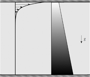
The ocean surface boundary layer is characterized by intense mixing and homogenized properties. Formed by processes such as wind stress, oceanic circulation and wave breaking, it can extend to large depths by convection, and interaction between surface waves and ocean currents (D'Asaro Reference D'Asaro2014). The generation of surface waves was analysed initially by Miles (Reference Miles1957), who considered a shear flow in the air layer, overlying a quiescent water layer. Subsequent studies by Valenzuela (Reference Valenzuela1976), Kawai (Reference Kawai1979) and van Gastel, Janssen & Komen (Reference van Gastel, Janssen and Komen1985) have incorporated a shear flow in the water layer also, assuming it to be setup by wind stress. This wind drift velocity profile is observed to be logarithmic in field measurements (Bye Reference Bye1965; Churchill & Csanady Reference Churchill and Csanady1983) and is characterized by the wind drift layer depth,  $h_w$ (typically much smaller than the depth of the ocean) and the surface velocity, $U_s$ ( ${\sim }3\,\%\text {--}4\,\%$ of wind speed). In the current study, we investigate the effects of the wind drift velocity profile on superharmonic generation by internal wave triadic resonances. Specifically, we consider an exponential velocity profile (Zeisel, Stiassnie & Agnon Reference Zeisel, Stiassnie and Agnon2008; Young & Wolfe Reference Young and Wolfe2014); it is both amenable to analytical calculations and provides results qualitatively similar to more realistic velocity profiles (Morland, Saffman & Yuen Reference Morland, Saffman and Yuen1991; Young & Wolfe Reference Young and Wolfe2014). The exponential background velocity profile in the ocean is assumed to be,
 \begin{equation} U(z) = \delta \exp\left(\frac{z-1}{\xi}\right),\quad 0\leqslant z \leqslant 1 ,\end{equation}
where  $\delta = U_s/(NH)$ and $\xi = L_s/H$ are as defined in § 2.2. Here, $U(z)$ is maximum at the free surface $(z=1)$ and negligible at the ocean bottom $(z=0)$. Unlike in § 2.2, $\delta$ is not necessarily assumed small in this section. As a result, the Richardson number $Ri = N^{2} L_s^{2}/U_s^{2}$ is allowed to assume arbitrary values. As shown in Appendix A, the dispersion curves and vertical mode shapes (governed by (2.5)) in the presence of the background flow in (3.1) can be analytically obtained. The dispersion curves in the presence of background flow are not symmetric about $\omega = 0$ (figure 2), and the cograde (modes that travel faster than the maximum background flow velocity) and retrograde (modes that travel slower than the minimum background flow velocity) modes have to be treated separately. For the cograde modes, the phase velocity rapidly approaches the asymptotic value of $U(1)$ as the mode number is increased, while the approach to $U(0)$ for retrograde modes is relatively slower (figure 2b). With respect to mode shapes, weak shear has a weak influence (figure 3a), while finite shear tends to accumulate zero crossings close to the boundaries (upper boundary for cograde modes and lower boundary for retrograde modes, see figure 3b,c). Owing to this accumulation, different mode shapes tend to look similar over most of the domain except near the boundaries (cograde modes 2 and 3 in figure 3(b), for example), with similar phase speeds (figure 2b). Consequently, the difference in the vertical structures of various high modes is not significant in most part of the domain, and resonant interaction between such modes is crucial to consider (Tung, Ko & Chang Reference Tung, Ko and Chang1981).

Figure 2. Dispersion curves for different mode numbers in a uniform stratification for (a)  $Ri = \infty$ and (b) $Ri = 1$. In each panel, the black, blue and red colours correspond to mode numbers $n = 1$, 2 and 3, respectively.

Figure 3. Mode shapes in a uniform stratification with an exponential background velocity profile (3.1) for (a)  $Ri = \infty$ (continuous lines, no shear), $Ri = 10^{5}$ (hollow circles, weak shear), (b) $Ri = 1$ (finite shear, cograde modes) and (c) $Ri = 1$ (finite shear, retrograde modes). In each panel, mode numbers $n =$1 (black), 2 (blue) and 3 (red) are shown.
In addition to the discrete modes shown in figure 3, there exists a singular continuous spectrum of modes whose phase speed matches with the background flow velocity at some  $z$, namely the critical layer (Banks et al. Reference Banks, Drazin and Zaturska1976; Jose et al. Reference Jose, Roy, Bale and Govindarajan2015). In this study, we will not consider such continuous spectrum solutions, for either the primary modes at frequency $\omega$ or the superharmonic modes at frequency $2\omega$. Hence, owing to the non-interaction theorem (Eliassen & Palm Reference Eliassen and Palm1961), no energy or momentum exchange between internal waves and the background flow can occur, up to at least $O(\epsilon ^{2})$ (Tung et al. Reference Tung, Ko and Chang1981).
3.1. Weak shear limit
We start by evaluating the asymptotic weak shear limit solutions of § 2.2 for representative modal combinations, verify if the predicted new resonances occur in the presence of shear and finally compare the asymptotic theory with numerical solutions. The conditions for divergence of the  $O(\epsilon ^{2})$ superharmonic wave field give the triadic resonance criteria for the interaction between modes $m,n$ at frequency $\omega$ and the superharmonic wave at frequency $2\omega$. The weak shear asymptotic theory in § 2.2 suggests that modes $m$ and $n$ at frequency $\omega$ and mode $q$ at frequency $2\omega$ are in triadic resonance if and only if $k_m + k_n = k_q$, where $q = |m-n|$ if there is no shear, and $q$ being any integer less than or equal to $\displaystyle \lfloor (m+n-1)/2\rfloor$ in the presence of a weak shear with $\upsilon ''(z) \neq 0$ somewhere in the domain. While such triadic resonances can occur only for $m/3< n<3m$ with no shear (Thorpe Reference Thorpe1966), no such restrictions exist in the presence of a shear flow. In other words, all the intersection points in figure 1(a) for a uniform stratification become triadic resonances in the presence of a weak shear.
Figure 4 shows the amplitude of the superharmonic wave (maximum value of  $\bar {h}_{mn}(z)$, which is governed by (2.12)) for representative modal interactions of $(m,n) = (2,3)$ and $(2,5)$, plotted as a function of the primary wave frequency $\omega$. For $(m,n) = (2,3)$, $\bar {h}_{mn}^{max}$ becomes infinitely large only at $\omega \approx 0.468$ for $Ri = \infty$ (no shear), with the superharmonic internal wave being of mode number $q = |m-n| = 1$ (blue curve in figure 4a). In the presence of weak shear ( $Ri = 10^{7}$), an additional divergence of $\bar {h}_{mn}^{max}$ appears at $\omega \approx 0.327$, which is the location where $k_q = k_m+k_n$ is satisfied with $q = 2$. Both the weak shear asymptotic theory (§ 2.2) and fully numerical solution of (2.12) confirm that triadic resonance occurs at both $\omega \approx 0.468$ and $0.327$. For $(m,n) = (2,5)$, while only one resonance location exists ( $\omega \approx 0.285$) with no shear (blue curve in figure 4b), two additional divergence locations appear with weak shear (grey dashed curve in figure 4b). The weak shear asymptotic theory is again shown to faithfully recover the new divergences (and hence triadic resonances) in the presence of weak shear for $(m,n)$ being equal to $(2,5)$ (black dotted curve in figure 4b). In summary, figure 4 confirms the main conclusion from the weak shear asymptotic theory for two representative modal interactions: in the presence of arbitrarily weak shear, additional triadic resonance locations emerge at all the locations where the horizontal wavenumber condition is satisfied. In addition, we also verified that divergence of $\bar {h}_{mn}^{max}$ due to triadic resonances resulting from self-interaction is also possible in the presence of weak shear.

Figure 4. Superharmonic wave amplitude  $\log _{10}[\bar {h}_{mn}^{max}]$ (2.12) plotted as a function of primary wave frequency $\omega$ at $Ri=\infty$ (no shear, shown in blue) and $Ri=10^{7}$ (asymptotics, numerics), for representative modal interactions specified by $(m,n) = (a)$ $(2,3)$, (b) $(2,5)$. The insets show a zoomed-in view of the additional divergences that occur in the presence of weak shear.
3.2. Finite shear
At finite shear, while it is possible to take a semi-analytical approach to solve (2.5) and (2.12) for the exponential background velocity profile (Appendix A), we present fully numerical solutions of (2.12) in this subsection owing to the simplicity in obtaining them. Using the shooting method alongside the fourth-order Runge–Kutta scheme to march from  $z = 0$ to $z = 1$, (2.5) is numerically solved to obtain the horizontal wavenumbers and the vertical mode shapes of different modes at a given primary wave frequency $\omega$. The boundary-value problem in (2.12) is then solved using a second-order finite difference scheme to obtain the superharmonic vertical structure $\bar {h}_{mn}(z)$ for different $(m,n)$ interactions. In the parameter space of $(\omega , Ri) \in [0.01, 0.99] \times [0.50, 10^{7}]$, we calculate the amplitude of the superharmonic wave ( $\bar {h}_{mn}^{max}$) and identify divergences via peaks in $\bar {h}_{mn}^{max}$ which become stronger with finer resolution in $\omega$. The superharmonic wave mode number ( $q$) is calculated throughout the parameter space using the number of zero crossings in the vertical structure of $\bar {h}_{mn}(z)$. It is worth pointing out that for $\omega >0.50$, while the superharmonic frequency is evanescent for $Ri = \infty$, propagating superharmonic internal wave modes exist for finite $Ri$ (Bell Reference Bell1974).
The distributions of  $\log _{10}[\bar {h}_{mn}^{max}]$ on the $(\omega , Ri)$ plane for three representative cograde modal interactions $(m,n) = (1,2)$, $(2,3)$ and $(2,2)$ are shown in figure 5(a–c). The divergence locations in the $\log _{10}[\bar {h}_{mn}^{max}]$ vs $\omega$ plot (like in figure 4) from different $Ri$ form the ‘divergence curves’ in figure 5. All the points along these divergence curves represent triadic resonance locations. In the limit of very large $Ri$, the divergence curves occur at locations predicted by the weak shear asymptotic theory (see hollow circles in figure 5a–c). For $(m,n) = (1,2)$, the triadic resonance between modes 1 and 2 at frequency $\omega$ and mode-1 at frequency $2\omega$ occurs at all values of $Ri$, with $\omega$ being at $0.395$ at large $Ri$ and increasing towards $0.482$ at $Ri = 0.50$ (figure 5a). For $(m,n) = (2,3)$, two different divergence locations are predicted in the weak shear limit, and they are observed to extend as divergence curves over a wide range of $Ri$. Similar to what was observed for $(m,n) = (1,2)$, the divergence curve corresponding to a mode-2 superharmonic internal wave deviates slightly from its weak shear limit location when $Ri$ reaches small values. In contrast, the divergence curve corresponding to the mode-1 superharmonic internal wave departs significantly from its $\omega$ value in the weak shear limit as $Ri$ becomes small. Interestingly, it does not even seem to extend all the way to $Ri = 0.50$. A similar behaviour is observed in the self-interaction case presented in figure 5(c), where the divergence curve associated with a mode-1 superharmonic internal wave goes from $\omega \approx 0.447$ at weak shear and towards large $\omega$ at $Ri\approx 1.50$ ( $\omega \approx 0.719$). It is worth recalling from § 2.2 that resonance due to self-interaction is not possible at all if there is no shear.

Figure 5. Contour plot of  $\log _{10}[\bar {h}_{mn}^{max}]$ for $(m,n) = (a)$ $(1,2)$, (b) $(2,3)$, (c) $(2,2)$, plotted on the plane of primary wave frequency $\omega$ on the $x$-axis and Richardson number $Ri$ on the $y$-axis. Hollow circles at $Ri = 10^{7}$ indicate the locations of divergence calculated from weak shear asymptotic theory. The mode number of the superharmonic internal wave at the divergence locations is indicated by the encircled numbers next to the corresponding divergence curves. Panels (d–f) are zoomed-in views of (a–c), respectively, in the regions of small $Ri$.
$Ri$.
Figure 5(a–c) shows that the primary wave frequency at the triadic resonance locations deviates very little from its weak shear limit value if  $Ri$ is larger than approximately $10^{2}$. For $Ri<10^{2}$, the divergence curves explore a larger range of primary wave frequencies, even extending to values for which the superharmonic frequency would be evanescent if there was no shear. To closely investigate the small $Ri$ region ( $0.50\leqslant Ri\leqslant 5$), figure 5(d–f) shows zoomed-in views of figure 5(a–c), respectively. For $(m,n) = (1,2)$, triadic resonance of the primary waves with the mode-1 superharmonic wave occurs at around $\omega \approx 0.482$ for small $Ri$ close to $0.50$, which is not far from the resonant value of $\omega \approx 0.395$ for $Ri\to \infty$. Similarly, the triadic resonance associated with the mode-2 superharmonic wave for $(m,n) = (2,3)$ occurs at similar $\omega$ for $Ri = 0.50$ and $Ri\to \infty$. In contrast, the triadic resonance associated with the mode-1 superharmonic wave ceases to exist below a cutoff $Ri$ of $2.94$ (figure 5e). Interestingly, for a given $Ri$ larger than (but in the vicinity of) $2.94$, resonant generation of a mode-1 superharmonic internal wave occurs at two different values of $\omega$. For example, triadic resonance with the mode-1 superharmonic internal wave occurs at $\omega \approx 0.743$ and $0.816$ for $Ri \approx 2.98$, and at $\omega \approx 0.587$ and $0.982$ for $Ri \approx 4.89$. Thus, for a finite range of $Ri\in (2.94,5.01)$, there exists two different $\omega$ values at which modes 2 and 3 at $\omega$ and mode-1 at 2 $\omega$ are in triadic resonance. A similar behaviour is observed with the triadic resonance between a self-interacting mode-2 at $\omega$ and mode-1 at $2\omega$ (figure 5f), The corresponding finite range of $Ri$ where two resonant $\omega$ values exist is $Ri\in (1.49,2.38)$. Finally, it is worth highlighting that weakly nonlinear effects seem to be stronger at smaller $Ri$ in general (including the regions away from divergence curves), as evidenced by the larger magnitudes of the superharmonic wave amplitude at small $Ri$ in figure 5(e,f).
As pointed out in § 2.2, a triadic resonance in the vicinity of  $\omega = 0$ appears for those $(m,n)$ for which $m+n$ is even, if a weak shear is present. This weak shear limit is indicated by the hollow circle at $\omega = 0$ and large $Ri$ in figure 5(c), where $m+n = 4$ is even. An increase in the superharmonic amplitude as one approaches the $\omega = 0$ axis is evident at all $Ri$, although we could not establish that a divergence curve exists in the neighbourhood for $\omega >0$. Upon further investigation, we found that the actual divergence curve occurs in the $\omega <0$ region for all $Ri$, which still represents a continuous extension of what occurs at $\omega = 0$ in the weak shear limit. An alternate view of this observation is that the $(2,2)$ triadic resonance interaction at $\omega =0$ for $Ri\to \infty$ extends to the finite $Ri$ region as a $(-2,-2)$ triadic resonance interaction at negative $\omega$ values, i.e. a retrograde–retrograde interaction. This aspect is further elucidated in figure 8.
In figure 6, we provide an interpretation of our observations for the  $(m,n) = (2,3)$ interaction (figure 5b,e) in the context of internal wave dispersion relation in the presence of shear. Like in figure 1(a), we plot the dispersion curves for the individual modes (shown in grey) and the $2\omega$ vs $(k_m+k_n)$ curves obtained from the dispersion curves for modes $m$ and $n$ at frequency $\omega$ (shown in black) for various $Ri$ in figure 6. At large $Ri$ ( $Ri = 100$ in figure 6a), $k_m+k_n = k_q$ ( $q$ is the mode number of the superharmonic wave) is satisfied at two different locations, each corresponding to $q = 1$ (blue dot) and $2$ (red dot). The corresponding primary wave frequencies are where divergence locations occur at $Ri = 100$ in figure 5(b), and are very close to those values predicted by the weak shear asymptotic theory. At $Ri = 5$, triadic resonance of the primary waves with the mode-1 superharmonic wave occurs at two different values of $2\omega$ (blue dots in figure 6b), again being consistent with the divergence locations at $Ri = 5$ in figure 5(b). As $Ri$ is further decreased to the previously identified cutoff value of $2.94$ (figure 6c), the two blue dots from figure 6(b) converge to a single location, and the mode-1 dispersion curve is now tangential to the $2\omega$ vs $(k_m+k_n)$ curve. At an even smaller value of $Ri$ ( ${=}0.50$ in figure 6d), triadic resonance with the mode-1 superharmonic wave is absent (no blue dots), in line with the observation from figure 5(e) that it ceases to exist below $Ri \approx 2.94$. Triadic resonance with the mode-2 superharmonic wave persists at all $Ri$, indicated by the red dots in each of figure 6(a–d). In summary, figure 6 establishes that divergence of the superharmonic wave amplitude (as shown in figure 5) occurs at the same locations where the horizontal wave numbers satisfy $k_m + k_n = k_q$, and hence represent triadic resonances. In addition, figure 6 also establishes that horizontal wavenumber condition is sufficient to ensure triadic resonance between the primary and superharmonic waves for finite shear too (§ 3.1 showed the same result in the weak shear limit).

Figure 6. Dispersion curves for mode numbers  $q=1$ to $3$ (grey lines) for (a) $Ri = 100$, (b) $Ri = 5$, (c) $Ri \approx 2.94$ and (d) $Ri = 0.50$. The black solid lines represent $2\omega$ vs $(k_m+k_n)$ with $(m,n) = (2,3)$. Points of intersection with the mode-1 and mode-2 superharmonic dispersion curves are indicated by the blue and red dots, respectively. In (d), the inset shows a zoomed-in view (with a modified quantity on the $x$-axis for better clarity) around the intersection point denoted by the red dot.
Extending the investigations in figures 5 and 6, we find that features such as multiple resonant  $\omega$ values at given $Ri$ and superharmonic mode number, and disappearance of some resonances below a cutoff $Ri$ are common for higher mode interactions too. These features can have significant implications for the total number of possible triadic resonances at various $Ri$, which we proceed to discuss in § 3.3.
3.3. Number of resonance locations
In oceanic settings like internal tide generation or scattering by ocean floor topography, a finite number of modes at the tidal frequency are excited, with the low modes often containing the most energy (Garrett & Kunze Reference Garrett and Kunze2007). In this subsection, we consider a scenario where a finite amount of energy is present in the first few modes at a fixed frequency, and investigate the total number of resonant interactions possible amongst them. Specifically, we consider all possible cograde–cograde interactions with  $(m,n)\leqslant (5,5)$, and plot all the corresponding divergence curves (obtained as locations where $k_m + k_n = k_q$ is satisfied) on the $\omega \text {--}Ri$ plane (figure 7a). All the divergence curves emerge from the weak shear limit (blue dots at large $Ri$), and expand towards other frequencies as $Ri$ is decreased. While some of them extend all the way to $Ri = 0.5$, others have a cutoff $Ri$ below which the corresponding resonances do not exist. As pointed out in § 3.2, some of the divergence curves occur at two different primary wave frequencies at a given $Ri$ within a particular range. In this range of $Ri$ (roughly around 1 to 100), the divergence curves extend over a large frequency range, which is in contrast with what happens at very large and very small $Ri$. Accounting for primary modes up to 10 (figure 7b), it becomes evident that almost every primary wave frequency corresponds to some resonant interaction for a finite band of $Ri$. Owing to existence of a cutoff $Ri$ for several of the interactions, only a few interactions are possible as $Ri$ approaches 0.5.

Figure 7. Resonance locations for all the cograde modal interactions amongst (a)  $(m,n) \leqslant (5,5)$ and (b) $(m,n) \leqslant (10,10)$, in the plane of primary wave frequency $\omega$ and Richardson number $Ri$. Number of resonance locations ( $N_R$) shown at different Richardson numbers ( $Ri$) for all the cograde modal interactions (c) $(m,n) \leqslant (5,5)$ and (d) $(m,n) \leqslant (10,10)$. In (a,b), blue dots indicate the resonance locations in the weak shear limit ( $Ri\to \infty$). In (c,d), the red and blue dots indicate $N_R$ in the weak shear and no shear limits, respectively.
For a given  $Ri$, the total number of resonant interactions ( $N_R$) over the entire range of $\omega \in [0,1]$ is calculated from the plots in figure 7(a,b), and $N_R$ is subsequently plotted as a function of $Ri$ in the bottom row of figure 7. As already pointed out, the number of resonances in the weak shear limit ( $Ri\to \infty$) is much larger than the no shear limit. In figure 7(c), which corresponds to interactions amongst the first 5 modes, the weak shear and no shear limits are shown by the red and blue dots, respectively. Considering primary wave frequencies in the range $[0,1]$, $N_R$ remains at $33$ for $63\leqslant Ri<\infty$, and starts to increase with a further decrease in $Ri$. It attains a maximum of $35$ in the interval of $16.26\leqslant Ri\leqslant 26.38$, before decreasing towards $10$ at $Ri \approx 1.19$. $N_R$ then remains at $10$ for $0.5\leqslant Ri\leqslant 1.19$. Considering a larger range of $\omega$ ( $\omega \in [0,1.5]$, shown in black), $N_R$ increases from its weak shear limit at a larger $Ri$ of $268.79$, and also attains a larger peak of $N_R = 45$ at $Ri \approx 32.01$. Increasing the maximum mode number considered to 10, a similar trend in $N_R$ vs $Ri$ is observed, but with a larger value of $Ri$ at which $N_R$ deviates from its weak shear limit (figure 7d).
In summary of figure 7, we have identified a finite range of  $Ri$ over which resonant interactions occur at a significantly wider range of primary wave frequencies than for large and small $Ri$. In addition, the total number of possible resonant interactions attains a maximum for intermediate $Ri$ of $O(10)$, before decreasing towards relatively small values at small $Ri$.
$Ri$.  $N_R$ at small $Ri$, while being much smaller than the weak shear limit, is still larger than the number of resonances in the no shear limit.
Due to symmetry breaking by the introduction of shear, retrograde–retrograde and mixed (cograde–retrograde) interactions behave differently from cograde–cograde interactions. To elucidate this, we show the contour plots of  $\log _{10}[\bar {h}_{mn}^{max}]$ for representative modal interactions of $(m,n) = (-2,-4)$, $(3,-5)$ and $(-1,4)$ in figures 8(a)–8(c), respectively. Here, a negative mode number $-m$ indicates a retrograde mode with mode number $m$. Unlike the dispersion curves of cograde modes (see figure 6, for example), the dispersion curves of retrograde modes are bounded by a maximum frequency, whose magnitude increases with $Ri$ and approaches $\omega = 1$ in the limit of no shear (Bell Reference Bell1974). This restricts the maximum primary wave frequency at which divergence curves can occur to $\omega = 0.5$, thus restricting the primary wave frequency axis to $\omega \in [0,0.5]$ in figure 8.

Figure 8. Contour plot of  $\log _{10}[\bar {h}_{mn}^{max}]$ similar to figure 5 but for representative (a) retrograde modal interaction $(m,n) = (-2, -4)$, (b) mixed modal interaction $(m, n) = (3, -5)$, and (c) mixed modal interaction $(m, n) = (-1, 4)$, plotted on the plane of primary wave frequency $\omega$ on the $x$-axis and Richardson number $Ri$ on the $y$-axis. Hollow circles at $Ri = 10^{7}$ indicate the locations of divergence calculated from weak shear asymptotic theory. The mode number of the superharmonic internal wave at the divergence locations is indicated by the encircled numbers next to the corresponding divergence curves. The negative sign before mode number indicates that it is a retrograde mode.
In the retrograde–retrograde interaction of  $(m,n) = (-2,-4)$ (figure 8a), three divergence curves emerge at $Ri\to \infty$ from the resonance locations predicted by the weak shear asymptotic theory (hollow circles), including one from $\omega = 0$. It is worth highlighting that the weak shear resonances occur at locations where the horizontal resonance condition is satisfied with no shear (§ 2.2), thus giving rise to the same resonance-emerging locations for cograde–cograde and retrograde–retrograde interactions. All the three divergence curves extend all the way to $Ri = 0.5$, with noticeable deviations from the weak shear limit. Interestingly, further investigations revealed that all the retrograde–retrograde resonance interactions that occur in the weak shear limit extend all the way to $Ri = 0.5$. This is in contrast to cograde–cograde interactions, some of which were shown to have a cutoff $Ri$ below which they do not exist. As was pointed out for even $m+n$ in cograde–cograde interactions (figure 5c), while a signature of the weak shear resonance at $\omega = 0$ was present in the form of enhanced superharmonic amplitudes, no divergence curve was actually detected (figure 5c). It turns out that the $\omega = 0$ resonances from the weak shear limit become retrograde–retrograde resonances for finite $Ri$, which explains the occurrence of a divergence curve with a retrograde mode 3 superharmonic wave in figure 8(a).
For the cograde–retrograde mixed interaction of  $(m, n) = (3, -5)$ (figure 8b), a divergence curve (with the superharmonic wave being a retrograde mode 1) appears in the vicinity of $\omega = 0$ at large $Ri$, emerging from the weak shear limit of $\omega =0$ that is possible due to even $m+n$. While the resonance at $Ri = 10^{7}$ is not very close to $\omega = 0$, we confirmed with further investigations for $Ri>10^{7}$ that the resonance location approaches $\omega = 0$ as $Ri$ is made even larger. This divergence curve extends all the way to $Ri = 0.5$, with its location being at $\omega \approx 0.416$ at $Ri = 0.5$. In addition, a new divergence curve (with the superharmonic wave being a retrograde mode 2) emerges from $(\omega , Ri) = (0, 2.42)$; the corresponding resonance has no weak shear counterpart. Such an occurrence of a new resonance at finite $Ri$ and $\omega = 0$ is observed only for mixed interactions. This new divergence curve is present at all $Ri\leqslant 2.42$, occurring at $\omega \approx 0.304$ for $Ri = 0.5$. Finally, for the mixed interaction case of $(m,n) = (-1, 4)$ (figure 8c), a single divergence curve is observed, and it emerges from the weak shear limit of $\omega \approx 0.395$. Unlike for the examples in figure 8(a,b), the resonance in figure 8(c) has a cutoff $Ri$ of $5.01$ below which it does not occur.
Having investigated representative retrograde–retrograde and mixed interactions in figure 8, and recognizing that they are quite different from cograde–cograde interactions, we proceed to reproduce the calculations in figures 7(a) and 7(c) in the presence of all interactions. Specifically, considering all possible interactions between cograde and retrograde mode numbers up to 5, we plot all the divergence curves on the  $\omega \text {--}Ri$ plane, with the colour indicating the type of interaction (figure 9a). The divergence curves corresponding to cograde–cograde interactions are reproduced from figure 7(a). All the divergence curves associated with retrograde–retrograde interactions extend all the way from their weak shear limit to $Ri = 0.5$, with quite a few of them emerging from $\omega = 0$ at $Ri\to \infty$. Interestingly, the $\omega = 0$ resonances expand towards larger values of $\omega$ as $Ri$ is decreased, thus making a significant range of $\omega \in [0,0.5]$ susceptible to retrograde–retrograde resonances at small $Ri$. Mixed interactions are fewer in number compared with other interactions at large $Ri$, but new resonances emerge at finite $Ri$, a feature that is absent for cograde–cograde and retrograde–retrograde interactions.

Figure 9. (a) Resonance locations for all the modal interactions amongst  $(|m|,|n|)\leqslant (5,5)$ i.e. for cograde, retrograde and mixed interactions, in the primary wave frequency $\omega$ and Richardson number $Ri$ plane. The blue dots indicate resonance locations in the weak shear limit. (b) Number of resonance locations ( $N_R$) plotted as a function of Richardson number( $Ri$) for all the modal interactions amongst $(|m|,|n|)\leqslant (5,5)$. The red and blue dots indicate the total number of resonance locations in the weak shear and no shear limits, respectively.
As in figure 7(c), we plot the total number of resonances ( $N_R$) as a function of $Ri$, including the contributions from all types of interactions (figure 9b). While the cograde–cograde contribution is reproduced (and already discussed) from figure 7(c), the retrograde–retrograde contribution is observed to be significant and invariant with $Ri$ (blue markers in figure 9b). The latter feature can be understood from figure 9(a), where all the retrograde–retrograde resonances extended all the way from $Ri\to \infty$ to $Ri = 0.5$. The number of mixed interactions is relatively small at large $Ri$, but increases noticeably once $Ri$ is decreased below a value of around $23.95$. At small $Ri$ of $O(1)$, the retrograde–retrograde contribution dominates, while the number of mixed interactions has overtaken the number of cograde–cograde interactions. In terms of the total number of resonances, $N_R$ remains more or less constant at its weak shear limit value of $85$ for $Ri\geqslant 63$, which is much larger than the no-shear value of $14$. Upon a decrease in $Ri$ below $63$,
$63$,  $N_R$ increases, as already observed for cograde–cograde interactions in 7(c). At small $Ri$, owing to the new resonances from mixed interactions, $N_R$ does not drop as significantly as the number of cograde–cograde interactions, and has a value of $73$ at $Ri = 0.5$. Finally, increasing the considered range of primary wave frequencies to $\omega \leqslant 1.5$ noticeably increases the maximum value of $N_R$ due to its influence on the cograde–cograde interactions at finite $Ri$, but has little effect on $N_R$ at small $Ri$.
$Ri$.
In summary, the total number of resonances with shear is significantly larger than that without shear, and attains a maximum at a  $Ri\approx 17.91$, Its value at small $Ri$ is comparable to its weak shear limit owing to the emergence of new mixed interaction resonances at finite $Ri$. Furthermore, it is noteworthy that the range of primary wave frequencies that are susceptible to resonances becomes very large at finite $Ri$ due to cograde–cograde interactions, and also occupies a significant range of $\omega \in [0,0.5]$ at small $Ri$ mainly due to retrograde–retrograde interactions.
4. Discussion and conclusions
In this study, triadic resonance resulting from interaction between discrete internal wave modes at the same frequency in a two-dimensional, uniformly stratified shear flow were considered. For a linear (primary) wave field comprising a series of modes at the same frequency  $\omega$, superharmonic (frequency $2\omega$) and mean-flow (frequency zero) terms constitute the weakly nonlinear solutions. At certain primary wave frequencies, the amplitude of the superharmonic term diverges as a result of triadic resonance between two primary modes and a superharmonic secondary mode. In the no shear limit, primary modes $m$ and $n$ at frequency $\omega$ are in triadic resonance with mode $q$ at frequency $2\omega$ if $k_m+k_n = k_q$ and $q = |m-n|$ are satisfied, where $k_i$ denotes the horizontal wavenumber of mode $i$ at the corresponding frequency (Thorpe Reference Thorpe1966). Here, we developed an asymptotic theory to investigate the influence of weak shear on the aforementioned triadic resonances. We find that, unlike in the no shear limit, the horizontal wavenumber condition of $k_m + k_n = k_q$ alone is sufficient to ensure a resonant interaction, independent of the superharmonic wave mode number $q$. As a result, several more resonances, which include self interactions, occur in the presence of an arbitrarily weak shear when compared with the no shear limit. The locations of these resonances can be traced back to those primary wave frequencies at which $k_m+k_n = k_q$ is satisfied in the no shear limit, including some at the seemingly trivial case of $\omega = 0$.
In § 3, we extended our investigations to finite shear by numerically solving the equations governing the weakly nonlinear superharmonic wave field. Specifically, an ocean-like exponential velocity profile was considered, and a systematic study on the effects of Richardson number  $Ri$ was performed. Here, $Ri\to \infty$ corresponds to the weak shear limit, and our study spans a wide range of $Ri$ all the way to $Ri = 0.5$. On the ( $\omega , Ri$) plane, the superharmonic wave amplitude diverges at locations of resonance, and the locus of all such points corresponding to a particular superharmonic internal wave of mode number $q$, is termed as a divergence curve of mode number $q$. For cograde–cograde interactions, a cutoff $Ri$ exists for a large number of divergence curves and only a few among all the divergence curves extend from $Ri\to \infty$ to $Ri = 0.5$. In addition, for a finite range of $Ri$ (roughly around 1–100) above the cutoff $Ri$ for a particular modal interaction, resonance occurs at two different primary wave frequencies at a given $Ri$. For retrograde–retrograde interactions, all the resonances that occur for $Ri\to \infty$ extend all the way to $Ri = 0.5$ without the occurrence of any cutoff $Ri$. Further, all the resonances that occur at zero primary wave frequency for $Ri\to \infty$ appear in retrograde–retrograde interactions at finite $\omega$ for finite $Ri$. For mixed interactions, a new feature of the emergence of new resonances at finite $Ri\sim O(10)$ is observed, thus contributing to an increase in the number of mixed interaction resonances at small $Ri$. The total (from cograde, retrograde and mixed interactions) number of resonance locations has a dramatic increase from the no shear limit to the weak shear limit ( $Ri\to \infty$), attains a maximum at moderate $Ri\,({\sim }O(10))$ and approaches a value that is not far from the weak shear limit value, at $Ri = 0.5$. This trend, particularly at small $Ri$, is understood as a consequence of a decrease and increase of the cograde–cograde and mixed resonant interactions, respectively, with $Ri$.
$Ri$.
Our conclusions based on the weak shear limit are potentially relevant for other inhomogeneous background conditions as well. Specifically, we showed that all the locations where the horizontal wavenumbers satisfy the triadic resonance condition in the absence of shear represent actual triadic resonances in the presence of an arbitrarily weak shear. A similar conclusion will hold if, instead of a weak shear, a weak non-uniformity in the stratification is introduced. This also explains why the previous study by Varma & Mathur (Reference Varma and Mathur2017) identified several more resonances in non-uniform stratifications compared with a uniform stratification. While Varma & Mathur (Reference Varma and Mathur2017) attributed the sufficiency of the horizontal resonance condition  $k_m + k_n = k_q$ to a non-orthogonality condition being satisfied by modal pairs in a non-uniform stratification, an equivalent perspective in our weak shear limit theory is that the coefficient of ‘ $\sin (\gamma z)/\sin \gamma$’ in (2.29) is non-zero. In summary, a weak inhomogeneity either in terms of shear or non-uniformity in stratification reduces the dimension of the spatial triadic resonance condition, and hence substantially increases the number of resonances compared with the case of uniform stratification with no shear.
A recent study by Biswas & Shukla (Reference Biswas and Shukla2021) directly used the sufficiency of frequency and horizontal wavenumber conditions to identify internal wave resonant triads in a uniformly stratified uniform shear flow. Considering primary modes  $(m,n)$ at the same frequency $\omega$, Biswas & Shukla (Reference Biswas and Shukla2021) investigated the stability of a few resonant triads (specifically five different $(m,n)$ combinations at a few arbitrarily chosen values of moderate $Ri$) that contained the superharmonic wave. In contrast to Biswas & Shukla (Reference Biswas and Shukla2021), we consider a realistic ocean-like background shear flow, and identify all possible low-mode interactions over a continuous range of $Ri$ spanning from weak to moderate to strong shear. An analysis of the amplitude evolution associated with all the resonant triads we identified in this study would be useful in determining their relative importance in a realistic internal wave field comprised of different modes.
Our study indicates that superharmonic generation due to triadic resonance is likely for a large range of primary wave frequencies, particularly at  $Ri\sim O(1\text {--}100)$, if a few different primary modes are simultaneously excited. In the future, it is important to consider the parameter values (Richardson number, frequency and mode numbers) for representative oceanic regimes (internal tides in the presence of wind forced shear flow or surface gravity wave-induced mean flow, wave–mean-flow interaction etc.) to study the extent to which superharmonic generation gets modified by background shear. It would further be interesting to study if the new resonances that occur due to shear can result in stronger secondary wave growth than those that are associated with the resonances in uniform stratification with no shear. This would require the derivation of amplitude evolution equations associated with the triadic resonances identified in this study. Additionally, incorporating the presence of background shear along with one or more of non-uniform stratification, background rotation, viscous and three-dimensional effects will take us a step closer to realistic oceanic settings. In a three-dimensional domain, additional classes of resonances (wave–vortex and vortex–vortex) analysed by Lelong & Riley (Reference Lelong and Riley1991) would also be relevant. The ideas in this paper may be relevant for triadic resonance with subharmonic waves too, including PSI i.e. apart from the effects of background shear on the already known subharmonic resonances (such as PSI), it is important to study if additional resonances occur due to background shear. Finally, it would also be interesting to study the effects of background shear on triadic resonances when critical layers, and hence the possibility of a continuous spectrum of modes, are present.
Acknowledgements
The authors acknowledge useful inputs from D. Varma during the early stages of this work.
Funding
The authors would also like to acknowledge support from (A) Indian Ministry of Human Resource Development under the SPARC programme (Sanction Order No. SPARC/2018-2019/P1213/SL), and (B) IIT Madras for its support of the ‘Geophysical Flows Lab’ research initiative under the Institute of Eminence framework.
Declaration of interests
The authors report no conflict of interest.
Appendix A. Analytical solution for an exponential velocity profile
To solve the governing equation for mode shapes, we transform (2.5) with an exponential background shear into a hypergeometric differential equation using the transformation given by Thorpe (Reference Thorpe1969). The general solution is then given by
 \begin{equation} \phi_j(z) = \mu^{s}(1-\mu)^{t}(\mathscr{C}_1F(p,q;r;\mu) + \mathscr{C}_2 \mu^{1-r} F(p-r+1,q-r+1;2-r;\mu)), \end{equation}
where
 $$\begin{align} \mu(z) &=\frac{\delta}{c_j}\exp\left(\frac{z-1}{\xi}\right),\quad s ={\pm} \lambda,\quad t = \frac{1}{2}(1\pm\sigma), \end{align}$$
 $$\begin{align}\lambda &= \frac{\xi}{c_j}\sqrt{\omega^{2} - 1}, \quad \sigma = \sqrt{1-4\xi^{2}/c_j^{2}}, \end{align}$$
 $$\begin{align}p &={\pm} \lambda+\tfrac{1}{2}(1\pm\sigma) \pm \sqrt{1+k_j^{2}\xi^{2}}, \notag\\ q &={\pm} \lambda+\tfrac{1}{2}(1\pm\sigma) \mp \sqrt{1+k_j^{2}\xi^{2}},\quad r = 1\pm 2\lambda. \end{align}$$
Here,  $\mathscr {C}_1$ and $\mathscr {C}_2$ are integration constants. This solution above is valid in the neighbourhood of the regular singular point $\mu = 0$, with radius of convergence $|\mu |<1$.
Applying the boundary conditions at  $z=0$ and $z=1$, we can write the dispersion relation as
 \begin{align} &\mu(1)^{1-r}F(p,q;r;\mu(0))F(p-r+1,q-r+1;2-r;\mu(1))\nonumber\\ &\quad -\mu(0)^{1-r}F(p,q;r;\mu(1))F(p-r+1,q-r+1;2-r;\mu(0))=0. \end{align}
At a particular primary wave frequency, evaluating the wavenumber analytically from (A5) is only possible in certain limiting cases. In general, various numerical root finding techniques such as the Newton–Raphson method can be easily employed to solve (A5).
Equation (2.12) is similar to the mode shape equation (2.5) but is inhomogeneous. The inhomogeneous part is obtained by substituting the wavenumber, found from (A5), and the mode shape from (A1) on the right-hand side of (2.12). Hence, the analytical solution of (2.12) includes integrals over the products of hypergeometric functions (i.e. nonlinear terms). These integrals can be evaluated or can be solved by numerical quadrature.
In summary, solving (2.5) and (2.12) can be carried out analytically but, in general, numerical methods are the only resort for finding the eigenvalues from (A5).
Appendix B. Coefficients of right-hand side terms in (2.24)
The coefficients of different terms on the right-hand side of (2.24) are as follows:
 $$\begin{align} \mathcal{A}(z) &={-}\dfrac{3}{4\omega^{3}}\left(\mathscr{A}_{mn}(z)+\mathscr{A}_{nm}(z)\right) - \dfrac{(1-4\omega^{2})}{2\omega^{2}}\left(\left(k_{m,1}+k_{n,1}\right)\left(k_{m,0}+k_{n,0}\right)\right)\bar{h}_{mn,0}(z), \end{align}$$
 $$\begin{align}\mathcal{B}(z) &= \frac{-\left(\mathscr{B}_{mn}(z)+\mathscr{B}_{nm}(z)\right)}{2\omega^{4}} - \frac{(k_{m,0}+k_{n,0})}{\omega}\left(\dfrac{(k_{m,0}-k_{n,0})^{2}}{\omega^{2}}+4k_{m,0}k_{n,0}\right)\bar{h}_{mn,0}(z), \end{align}$$
 $$\begin{align}\mathcal{C}(z) &={-}\frac{A_{m,0}A_{n,0}}{8\omega^{4}}\left(k_{m,0}k_{n,0}\left(k_{m,0}+k_{n,0}\right)^{2}+4 k_{m,0}k_{n,0}\left(k_{m,0}^{2}+k_{n,0}^{2}\right)\right)\phi_{m,0}(z)\phi_{n,0}(z), \end{align}$$
 $$\begin{align}\mathcal{D}(z) &={-}A_{m,0}A_{n,0}\dfrac{\left(k_{m,0}-k_{n,0}\right)}{4\omega^{2}}\left(k_{n,0}\phi_{m,0}'\phi_{n,0}-k_{m,0}\phi_{m,0}\phi_{n,0}'\right) -\frac{(k_{m,0}+k_{n,0})}{2\omega}\bar{h}_{mn,0}(z), \end{align}$$
 $$\begin{align}\mathcal{E}(z) &= A_{m,0}A_{n,0}\dfrac{k_{m,0}k_{n,0}}{2\omega^{2}}\phi_{m,0}\phi_{n,0}, \end{align}$$
where,
 \begin{align} \mathscr{A}_{mn}(z) &= \dfrac{\left(k_{m,0}^{2}-k_{n,0}^{2}\right)}{2}\left[A_{m,0}A_{n,0}\left(k_{n,0}\phi_{m,1}'\phi_{n,0} - k_{m,0}\phi_{m,1}\phi_{n,0}' + k_{n,1}\phi_{m,0}'\phi_{n,0}\right) \right.\nonumber\\ &\quad \left.+\left(A_{m,1}A_{n,0}+A_{m,0}A_{n,1}\right)k_{n,0}\phi_{m,0}'\phi_{n,0}\right]\nonumber\\ &\quad +A_{m,0}A_{n,0}k_{n,0}\left(k_{m,1}k_{m,0}-k_{n,1}k_{n,0}\right)\phi_{m,0}'\phi_{n,0}, \end{align}
and
 \begin{equation} \mathscr{B}_{mn}(z) = A_{m,0}A_{n,0}k_{n,0} (k_{m,0}^{3}-k_{n,0}^{3})\phi_{m,0}'\phi_{n,0}. \end{equation}


 Open access