


1 Introduction
Plumes containing bubbles, particles and droplets are present in both environmental and industrial applications. A few examples of environmental interest are settling sediment, volcanic eruption columns,  $\text{CO}_{2}$ ocean sequestration plumes, and rising oil droplets and gas bubbles from oil well blowouts (Freeth Reference Freeth1987; Baines & Sparks Reference Baines and Sparks2005; Baines Reference Baines2008; Socolofsky & Bhaumik Reference Socolofsky and Bhaumik2008; Woods Reference Woods2010; Socolofsky, Adams & Sherwood Reference Socolofsky, Adams and Sherwood2011; Huppert & Neufeld Reference Huppert and Neufeld2014; Wang et al. Reference Wang, Socolofsky, Breier and Seewald2016). Suspension-flow plumes differ from traditional single-fluid plumes in that the energy due to buoyant forcing is transmitted indirectly from the suspended phase to the continuous phase. The relative motion between the two phases introduces additional length and time scales; these must be included in the model formulation employed to predict plume behaviour, for example, when extending classic single-phase integral plume models (Morton, Taylor & Turner Reference Morton, Taylor and Turner1956) to multiphase plumes (Milgram Reference Milgram1983; Sun & Faeth Reference Sun and Faeth1986). Identifying such scales is non-trivial due to the complexity of particle–particle and particle–fluid interactions.
For the special case of air bubbles in water, empirical data collection has allowed accurate closure of predictive schemes (Lance & Bataille Reference Lance and Bataille1991; Risso & Ellingsen Reference Risso and Ellingsen2002; Mercado et al. Reference Mercado, Gomes, van Gils, Sun and Lohse2010; Almeras et al. Reference Almeras, Mathai, Lohse and Sun2017; Risso Reference Risso2018). However, the bubble-in-water plume can be quite different from other suspension-flow plumes of interest, because bubbles are far less dense than the ambient fluid (specific gravity of order  $10^{-3}$) and have negligible inertia. Other plumes of interest are droplets in water (specific gravity of order 1), solid particles in water (specific gravity of order 2 to 10), or liquid droplets in air (specific gravity of order $10^{3}$). Each of these different suspensions can behave quite differently than the others in terms of the interphase interactions. Empirical data are relatively scarce for these other suspension-flow plumes.
Recent progress in suspension flows (especially turbulent flows) offers the hope that predictive techniques will eventually describe overall plume behaviour from a direct description of the internal dynamics of particle–fluid coupling. To help support this strategy and address some of the open questions that remain about turbulent suspension flows (Balachandar & Eaton Reference Balachandar and Eaton2010; Guazzelli & Morris Reference Guazzelli and Morris2012), we take an observational approach herein, measuring the particle and fluid behaviours in a particle-laden plume. Because particles are dynamically quite different from air bubbles in water, we are curious to see how the two-phase kinematics and the interstitial fluid turbulence behave.
Both bubbles and particles have been shown to modulate the turbulent properties of multiphase flows in a manner sensitive to volume fraction ( $\unicode[STIX]{x1D719}$), particle Reynolds number ( $Re_{d}$) and particle Stokes number ( $St$). One starting point for understanding such turbulence modulation is the agitation of a quiescent fluid by bubbles or particles distributed homogeneously in space. This is often referred to as pseudo-turbulence (e.g. Lance & Bataille (Reference Lance and Bataille1991), Cartellier & Rivière (Reference Cartellier and Rivière2001)) as its characteristic scales are set by the bubble or particle wakes. Pseudo-turbulence is fundamentally anisotropic, with stronger velocity fluctuations aligned in the direction of suspended-phase motion ( $x_{1}$, typically vertical). Numerical simulations of pseudo-turbulence by Riboux, Legendre & Risso (Reference Riboux, Legendre and Risso2013) show that the velocity fluctuation energy spectrum has a slope of $k^{-3}$ for wavelengths smaller than the integral length scale; they also find that the integral length scale is the ratio of the bubble or particle diameter and the drag coefficient, $C_{d}$.
A recent topical review article by Risso (Reference Risso2018) provides a comprehensive summary of pseudo-turbulence due to a homogeneous swarm of bubbles rising in a quiescent medium. First, the turbulence intensity is anisotropic and is dominated by the vertical component. The probability density function (p.d.f.) of the vertical component is positively skewed due to the wake immediately behind each rising bubble, whereas the other two components are symmetrically distributed with exponential tails. Because the turbulent kinetic energy (TKE) production in suspension flows occurs at two length scales (first at the scale of bubble wakes and second at the scale of overall bubble population), the combination of the two results in a  $k^{-3}$ spectral subrange.
Previous laboratory (Hall et al. Reference Hall, Elenany, Zhu and Rajaratnam2010) and numerical (Azimi, Zhu & Rajaratnam Reference Azimi, Zhu and Rajaratnam2011, Reference Azimi, Zhu and Rajaratnam2012) studies have investigated the influence of particle size, particle concentration and nozzle size on the mean flow characteristics of sediment plumes. These authors considered fine to medium sized sand with diameters in the 0.1–0.8 mm range. Among all the observed differences between the particle plume and its single-phase counterpart, the nonlinear growth of plume width with downstream distances is a significant result; the two-phase plume initially spreads at approximately the same rate as single-phase plumes and then spreads at a lower rate beyond 60 nozzle diameters downstream. This change in the spreading rate affects all other mean flow variables as they are tied together by the continuity and momentum equations. In the present study, we consider the turbulent statistics of the two-phase plume in the initial spreading region. We choose to focus on the initial region because direct measurements of the plume turbulence are already lacking. Our results can be used for comparison in future studies looking at the region with a reduced plume growth rate.
To our knowledge, there are no existing studies examining turbulence in negatively buoyant particle plumes released into an unstratified, initially quiescent fluid. However, there are many studies of turbulence in bubble plumes with notable contributions coming from Soga & Rehmann (Reference Soga and Rehmann2004), Wain & Rehmann (Reference Wain and Rehmann2005), García & García (Reference García and García2006), Seol, Duncan & Socolofsky (Reference Seol, Duncan and Socolofsky2009), Simiano et al. (Reference Simiano, Lakehal and Lance2009) and Lai & Socolofsky (Reference Lai and Socolofsky2019). These investigations reveal different velocity characteristics at a different axial distance ( $x_{1}$) from the origin. Simiano et al. (Reference Simiano, Lakehal and Lance2009) examined the near-field characteristics ( $x_{1}/D<2$, where $D$ is the dynamic length scale to be defined in § 3.1) and showed that the meandering nature of bubbles influences the effective spreading, volume fraction and mean velocity profiles. Seol et al. (Reference Seol, Duncan and Socolofsky2009) and Lai & Socolofsky (Reference Lai and Socolofsky2019) focused on the far field ( $2<x_{1}/D<11$) turbulence characteristics, such as Reynolds stress, turbulent transport and TKE budget; their results will be used to compare with our particle plume data.
In recent years, computational fluid dynamics (known as CFD) has seen significant improvements in computational speed, domain size and in the flow complexities it can simulate. This in turn has allowed more accurate representations of flow physics in the simulations using approaches such as large eddy simulation (LES) and hybrid Reynolds-averaged Navier–Stokes (known as RANS) LES. To further develop and improve turbulence closure models in these approaches, a comprehensive database of canonical turbulent flows is needed. This need is especially relevant for multiphase flows in which a physics-based coupling model between the carrier and dispersed phase is critical to successful predictions. To this end, we offer a dataset of a heterogeneous particle plume with statistics of the turbulent velocity fluctuations up to the third order. Although boundary layer resolving direct numerical simulations (DNS) that resolve all relevant flow physics have been available for several years now, these simulations tend to be limited to homogeneous flows with periodic boundary conditions. It is necessary to validate closure models using data with flow heterogeneities as most industrial and engineering flows are inhomogeneous. This study represents an important step as practical particle-laden flows are often released from a point source.
Characterizing the turbulence statistics in a multiphase plume is challenging, primarily due to the difficulty in simultaneously measuring velocity in both phases. Traditional intrusive techniques such as hotwire anemometry suffer from the possibility of being damaged by the solid particles. Optical measurements from techniques such as particle image velocimetry (PIV) and laser Doppler anemometry are usually distorted due to the difference in optical properties of the two media. We overcome the distortion herein by carefully choosing two media with matched refractive indices.
This paper is organized as follows: § 2 provides a detailed description of the plume-generating facility and method for characterizing the two-phase flow. We report and discuss our experimental observations in § 3. Finally, § 4 provides the key conclusions from this work.
2 Experimental set-up and methodology
2.1 Plume facility
The plume experiments were conducted in a rectangular tank (80 cm deep  $\times$ 80 cm wide $\times$ 365 cm long) as described in Bordoloi & Variano (Reference Bordoloi and Variano2017). The tank was filled with tap water filtered to $5~\unicode[STIX]{x03BC}\text{m}$ and maintained using an ultraviolet (UV) purifier. Then 91.1 kg of commercial sodium chloride (Cargill Top-Flo) was mixed to yield a salt concentration of $0.04~\text{g}~\text{ml}^{-1}$. The resulting solution has density $\unicode[STIX]{x1D70C}_{s}=1.04~\text{g}~\text{cm}^{-3}$ and kinematic viscosity $\unicode[STIX]{x1D707}_{s}=1.059\times 10^{-3}~\text{Pa}~\text{s}$ (see table 1).

Figure 1. (a) Schematic of experimental facility and plume release mechanism (in inset), (b) regions of interest with specific dimensions, a picture of Teflon particles (inset A) and an illustration of two-dimensional transformation from world coordinates into the plume coordinates (inset B).
Table 1. Physical properties of particles and surrounding salt–water solution.
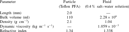
A schematic of the experimental set-up is shown in figure 1(a). The negatively buoyant plume was created by releasing 110 ml of cylindrical Neoflon PFA AP-202 (a copolymer of tetrafluoroethylene and perfluoroalkyl vinyl ether) from a height of 56.5 cm via a screw feed particle release mechanism (see figure 1b). The pellets are right circular cylinders with  $\text{length}=\text{diameter}=2~\text{mm}$ (see figure 1b-A). The physical properties of the solid particles and the surrounding salt solution are summarized in table 1. Because of the hydrophobic nature of PFA, the particles tend to trap and hold air bubbles when added to water. To prevent these air bubbles from entering the experiment, particles were presoaked in water in a separate container and rapidly stirred to dislodge all bubbles. Once the particles were free of air bubbles, they were placed in a funnel for eventual release into the quiescent salt–water mixture. The funnel was kept partially submerged 23 cm below the free surface through a nozzle with internal diameter $d_{0}=11.25~\text{mm}$ so that the particles did not contact air (see figure 1b). Particle release was governed by a motor-driven helical screw. Prior to release, the particles were held inside the funnel by the blades of the screw. Upon release, the motor rotated the screw at a constant rate of 0.5 r.p.m. operated via Lego Mindstorms software. The particle flux, $Q_{0}=7.5~\text{cm}^{3}~\text{s}^{-1}$ was measured by video recording the release of a known quantity of particles and measuring the time difference between the exit of the first and last particle from the funnel nozzle. Before each experiment, the tank fluid was seeded with optical tracers, specifically $13~\unicode[STIX]{x03BC}\text{m}$ silver-coated hollow glass spheres (SH400S20, Conduct-O-Fil, Potters Industries). Twenty plume releases provided a sufficient number of samples for the analysis described in § 3.
The plume release conditions for this study are parameterized into five non-dimensional numbers as suggested in Lai et al. (Reference Lai, Chan, Law and Adams2016) and are summarized in table 2. Here,  $u_{0}$ is the initial plume velocity computed from particle volume flux $Q_{0}$ and $u_{s}$ is the characteristic settling velocity of a particle. We measure the inlet volume fraction ( $\unicode[STIX]{x1D6FC}_{0}$) separately from a sample of 100 ml of tightly packed particle–water mixture. The velocity scale ( $u_{s}=0.23~\text{m}~\text{s}^{-1}$) is the terminal velocity of a single spherical particle in quiescent fluid and is computed using the standard Clift–Gauvin drag model for a sphere with volume equivalent to our particles. This value, inserted in the correction model proposed in Loth (Reference Loth2008), reduces significantly namely to $u_{s}=0.04~\text{m}~\text{s}^{-1}$. Because computing the drag on a non-spherical particle in intermediate Reynolds number is complex, we restrict our analysis to the standardized drag model for a spherical particle. Future work in which we focus on particle velocities will examine this issue in greater detail.
Table 2. Plume release parameters used in this study.
2.2 Refractive index matching
To measure the fluid velocity inside and around the plume, we matched the refractive index ( $n$) of the particle and fluid phases. A target refractive index of PFA ( $n\approx 1.34$) was achieved from an aqueous solution of commercial sodium chloride with a concentration of $0.04~\text{g}~\text{ml}^{-1}$. The refractive index of the solution was measured to be 1.338 using an ATAGO refractometer and found to match with the salinity versus
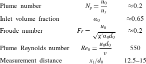
  $n$ prediction given in Tan & Huang (Reference Tan and Huang2015). Although the refractive indices of the two phases were matched, because of the scattering properties of PFA the particles appeared bright under the laser illumination. To limit the intensity of particles below the saturation threshold of the camera’s sensor we used a circular polarizer on each camera lens. Figure 2 shows example images of Teflon particles in different salinity water samples illuminated by a laser sheet ( $\text{wavelength}=532~\text{nm}$). The high-intensity elements in the images represent the particles intersected by the laser sheet. The low-intensity elements are the particles outside the laser-sheet plane. Fluid tracers (seen as tiny bright dots) are much more visible when particles and fluid have matched refractive indices (figure 2b compared to figure 2a). This difference is well demonstrated inside the dotted rectangle in each figure: tracers obstructed by the out-of-plane particles are much more visible inside the rectangle in figure 2(b).
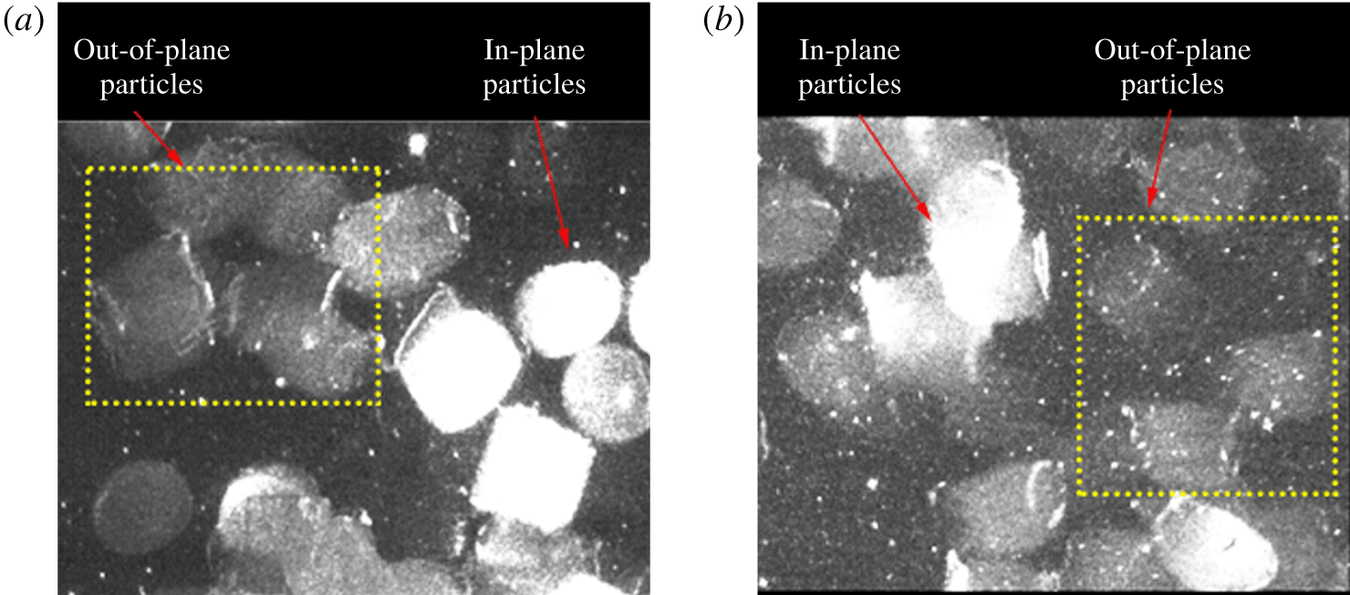
Figure 2. Teflon particles (large) and silver coated hollow glass spheres (small) illuminated by a 532 nm laser sheet in (a) pure water, (b) 0.4 % salt–water mixture.
2.3 Multiphase velocimetry
We performed stereoscopic particle image velocimetry (SPIV) to find the two-dimensional three-component (2D3C) velocity field of the fluid phase of the plume. The origin of our coordinate system is located at the tank centre. The plume is axisymmetric about the vertical axis, but we use Cartesian coordinates ( $x_{1}$, $x_{2}$, $x_{3}$) for our measurements as described in figure 1(b). Velocity measurement of the particle phase is currently underway and beyond the scope of this paper.
The  $x_{3}=0$ plane was illuminated with a laser sheet (1 mm thick at beam waist; Quantel/Big Sky Lasers, 532-nm double-pulse Nd-YAG). Two charge-coupled device (known as CCD) cameras (Imager PRO-X, $1600~\text{pixels}\times 1200~\text{pixels}$) were synchronized with the laser pulses. They were placed $\pm 55^{\circ }$ to the laser sheet (cf. $90^{\circ }$ for standard 2D2C PIV). To minimize distortion due to this angle, water-filled acrylic prisms were placed between the camera lenses and the tank walls. The cameras were mounted with Nikkor 105 mm lenses, circular polarizers and Scheimpflug adapters. The interframe delay ( $\unicode[STIX]{x0394}t$) was optimized to 0.5 ms. The PIV images were collected at a frequency of 14.0 Hz. The sampling frequency was chosen such that the Eulerian fluid motions were decorrelated based on the correlation coefficient computed from subsequent samples. This set-up gave approximately 50 independent samples during the steady-state phase of each experimental run. We performed a convergence test for all dominant statistical quantities discussed in § 3 and found them to converge within $\pm 4\,\%$ for 1000 independent samples.
2.3.1 Fluid-phase processing
Figure 3. Sample mean-subtracted instantaneous 2D3C velocity field in the fluid phase superposed with the particle image in the laboratory coordinate system. The vectors show the in-plane velocity ( $u_{1}$, $u_{2}$, $\text{m}~\text{s}^{-1}$), and the shades of red and green colours show the out-of-plane velocity component ( $u_{3}$, $\text{m}~\text{s}^{-1}$). The reference vector on the upper right corner corresponds to $0.5~\text{m}~\text{s}^{-1}$.
We computed the fluid-phase velocity field using DaVis 8.2 software (LaVision GmbH). Before SPIV processing, we performed stereo self-calibration to reduce disparity in the alignment between the laser sheet and the measurement plane to below 0.1 pixel. Tracers and particles in an image were separated by intensity thresholding; erosion and dilation were applied to isolate individual particles. Fluid velocity fields were obtained by masking particles and correlating tracer locations through multipass stereoscopic cross-correlation. The cross-correlation was applied with an initial interrogation window of  $64~\text{pixel}\times 64~\text{pixel}$ and a final window of $48~\text{pixel}\times 48~\text{pixel}$ with 50 % overlap, yielding a spacing between vectors of 0.7 mm. Interrogation windows were weighted according to the symmetric two-dimensional Gaussian function. Vectors were discarded based on universal outlier detection (Westerweel & Scarano Reference Westerweel and Scarano2005) and left as data gaps. Figure 3 shows a representative field of fluid velocity fluctuations superposed with the corresponding particle image (transformed into the lab coordinate system). The grid cells are colour-coded with the out-of-plane velocity component while the vectors show the in-plane velocity field.
2.3.2 Particle-phase processing
To estimate the particle number density across the plume, we conducted a series of additional image processing steps (see figure 4). First, the raw images were transformed from the camera coordinate system to the lab coordinate system using the stereoscopic mapping function. Small-size background noise features (including tracers) were removed using a simple median filter.
In stereo mapping, after transforming into the lab coordinate system, the section of the particle intersected by the laser sheet should overlap in both cameras. Figure 4(a) shows a sample instant with the two camera images overlayed. The high intensity regions in the image represent the intersection between the two camera images, whereas the low intensity background is from the out-of-plane particles captured in only one of the two cameras. We remove the background noise by setting an intensity threshold and convolving the two images. The result is shown in figure 4(b).
After inspecting our dataset, we find many instances where particles are nearly touching as exemplified in the lower left pair in the image. The non-uniform intensity gradients in the bordering regions among different particle pairs yielded different intensity gradients. A traditional intensity-gradient-based image segmentation therefore could not differentiate between two particles, and so we adopted a segmentation technique based on the watershed transform. The watershed transform treats an image as a topographic map with brighter intensity pixels as heights, and finds the separating line that runs along the ridges (Gonzalez & Woods Reference Gonzalez and Woods2007). The result, with individual particles identified with separate colours, is shown in figure 4(c). Since the area of a laser-intersected particle image is known a priori, we applied an area threshold to remove partially illuminated particles (which are out of the measurement plane). The centroids of particles identified from the final binary image are shown in figure 4(d).

Figure 4. Image processing steps leading from raw PIV image to centroid identification: sample image showing (a) particles from camera 1 and camera 2 blended into one image, (b) convolution of camera 1 image with camera 2 image, (c) image segmentation based on watershed transform and (d) final binary image with particle boundaries and located centroids in the laboratory coordinate system.
2.4 Coordinate transformation
Typically in jets and plumes the cross-stream velocity components ( $U_{2}$ and $U_{3}$) are smaller than the axial velocity component ( $U_{1}$) near the centreline. Thus, any small misalignment between the plume axis and the measurement axis could lead to a systematic bias in the measured $U_{2}$ and $U_{3}$. The scenario is schematically shown in inset B in figure 1(b) in a simplified $x_{1}{-}x_{2}$ plane in which the plume axis, $x_{1}$, makes an angle $\unicode[STIX]{x1D703}_{1}$ with the measurement axis $x_{1}^{\prime }$. For our data, if $\unicode[STIX]{x1D703}_{1}$ is defined the same way and if $\unicode[STIX]{x1D703}_{2}$ is the angle between the plume axis and the measurement axis on the $x_{1}{-}x_{3}$ plane, using axisymmetry and assuming that $\langle U_{2}\rangle ,\langle U_{3}\rangle =0$ at the plume centreline, the measured velocities can be transformed into the plume coordinate system via correction angles,
 $$\begin{eqnarray}\unicode[STIX]{x1D703}_{1}=\text{atan}\left(\frac{\langle U_{2}^{\prime }\rangle _{0}}{\langle U_{1}^{\prime }\rangle _{0}}\right),\quad \unicode[STIX]{x1D703}_{2}=\text{atan}\left(\frac{\langle U_{3}^{\prime }\rangle _{0}}{\langle U_{1}^{\prime }\rangle _{0}}\right).\end{eqnarray}$$
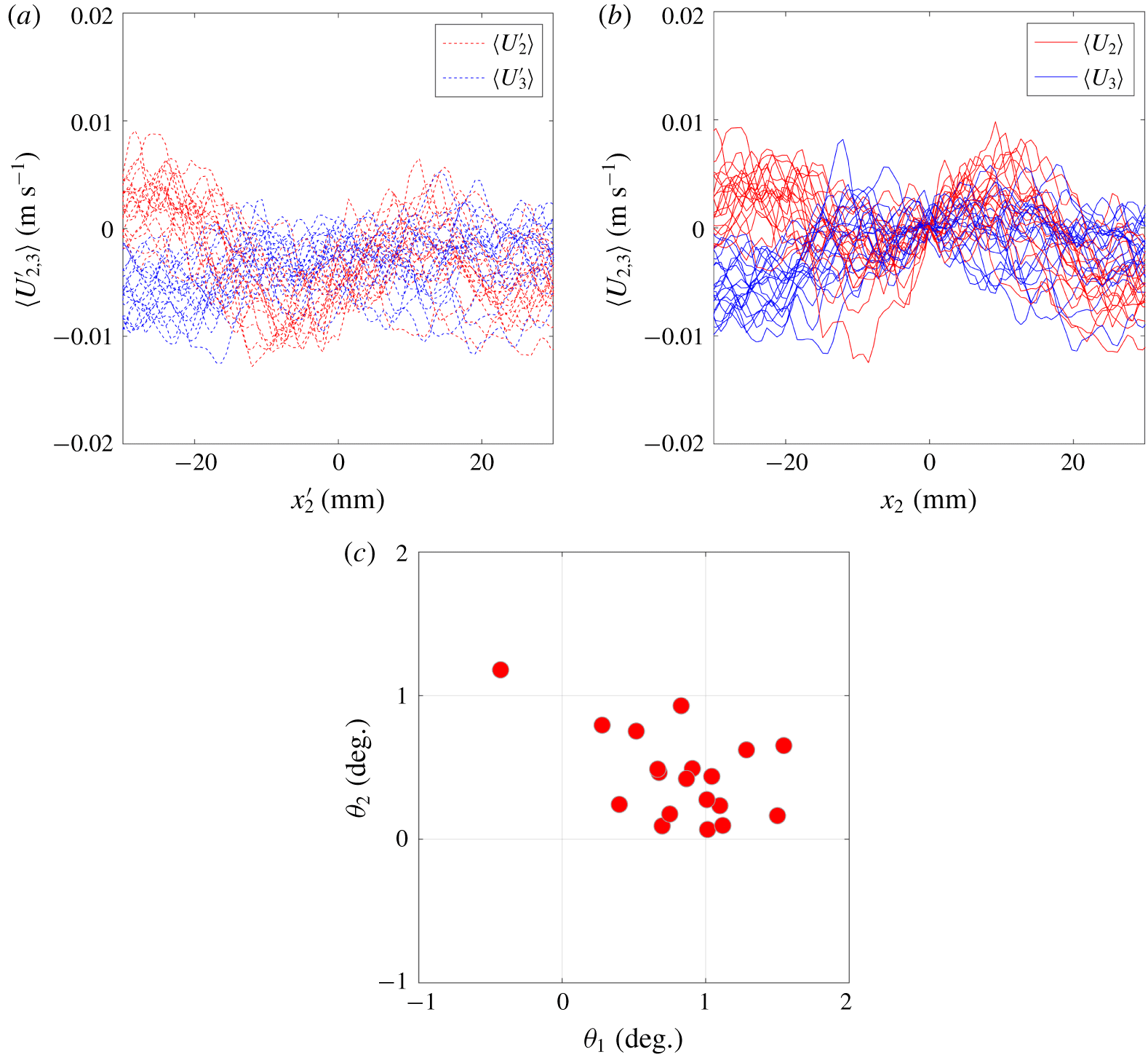
Figure 5. The radial and out-of-plane mean velocity components in (a) laboratory coordinate and (b) plume coordinate system averaged across the axial direction, and (c) mapping angles ( $\unicode[STIX]{x1D703}_{1}$ and $\unicode[STIX]{x1D703}_{2}$) based on (2.1).
The measurement bias in  $U_{2}$ and $U_{3}$ at the plume centreline are captured in figure 5(a) that shows the respective mean radial profiles, $\langle U_{2}^{\prime }\rangle$ and $\langle U_{3}^{\prime }\rangle$. We perform this transformation for the 20 replicate datasets independently with correction angles ( $\unicode[STIX]{x1D703}_{1}$, $\unicode[STIX]{x1D703}_{2}$) reported in figure 5(c). The bias in the non-zero centreline velocities are reflected in $\unicode[STIX]{x1D703}_{1}$ and $\unicode[STIX]{x1D703}_{2}$ which are small and less than $1.5^{\circ }$. The two velocity components transformed into the plume coordinate systems are shown in figure 5(b). The analysis that follows will be in the plume coordinate system.
3 Results and discussion
3.1 Mean flow characteristics
We first characterize the mean interstitial fluid velocity based on approximately 1000 independent PIV snapshots. The mean axial velocity field  $\langle U_{1}(x_{1},x_{2})\rangle$ in dimensional form is shown in figure 6(a). The radial ( $x_{2}$) variations of $\langle U_{1}\rangle$ normalized by the local mean centreline velocity $\langle U_{c}(x_{1},0)\rangle$ (written as $U_{c}$ for simplicity from here onward) are shown in figure 6(b) at representative axial locations ( $12.9d_{0}<x_{1}<15.1d_{0}$) across our measurement region. The Gaussian plume radius, $b_{g}$, defined as the $x_{2}$ location where $\langle U_{1}\rangle =\text{e}^{-1}U_{c}$, is obtained via a nonlinear least squares fit of each measured profile to a normalized Gaussian function. The data closely follow the Gaussian curve (solid line in figure 6b), which is also seen in single- and multi-phase jets and plumes (Milgram Reference Milgram1983; Darisse, Lemay & Benaïssa Reference Darisse, Lemay and Benaïssa2012; Lai & Socolofsky Reference Lai and Socolofsky2019).

Figure 6. (a) Two-dimensional intensity field showing the local mean axial velocity ( $\langle U_{1}\rangle$, $\text{m}~\text{s}^{-1}$) across the PIV measurement region, (b) radial profiles of non-dimensional $\langle U_{1}\rangle /U_{c}$ at 45 axial locations ( $x_{1}/d_{0}$) indicated by the colourbar.
Next, we examine the axial decay of centreline velocity,  $U_{c}$, and the axial growth of Gaussian plume radius ( $b_{g}$) for a particle plume by comparing them to existing data from bubble plumes (see figure 7). For the purpose of comparison, we use two non-dimensional parameters: a velocity scale ( $u_{s}$) and a length scale ( $D=gQ_{0}/4\unicode[STIX]{x03C0}\unicode[STIX]{x1D6FC}_{0}^{2}u_{s}^{3}$). These are based on an integral model of bubble plumes (Bombardelli et al. Reference Bombardelli, Buscaglia, Rehmann, Rincon and Garcia2007), in which a constant $\unicode[STIX]{x1D6FC}_{0}=0.083$ is used as the entrainment coefficient. The computed entrainment coefficient of our particle plume to be presented later is different from this a priori constant. The velocity scale ( $u_{s}=0.23~\text{m}~\text{s}^{-1}$) is the terminal velocity of a single particle in quiescent fluid and is computed using a simple drag model (Clift, Grace & Weber Reference Clift, Grace and Weber1978). Based on $Q_{0}=7.5~\text{cm}^{3}~\text{s}^{-1}$, the length scale $D$ is approximately 6.8 cm. This situates our axial measurement region between $2{-}2.5D$.
The overall trends in both centreline velocity and plume radius show similarity between particle and bubble plumes. The axial variation of  $U_{c}/u_{s}$ in a particle plume is not measurable from our data, but we can say that it falls above the curve for bubble plumes (Lai & Socolofsky Reference Lai and Socolofsky2019) (see figure 7a). The dashed and solid lines in figure 7(a) are the $-1/3$ power law fits, with $A=2.05$ (current data, see inset) and $A=1.6$ (Lai & Socolofsky Reference Lai and Socolofsky2019). The variation of $b_{g}$ for all the data (including ours) is captured by the solid line ( $b_{g}/D=0.114x_{1}/D$) in figure 7(b). Within the limited axial extent ( ${\approx}0.5D$) of our measurement, the local spreading rate ( $\unicode[STIX]{x1D6FD}=\text{d}b_{g}/\text{d}x_{1}$) is difficult to estimate. However, justified based on the collapse of our data on the solid line in figure 7(b), we will use $\unicode[STIX]{x1D6FD}=0.114$ in the remaining analyses in this paper.
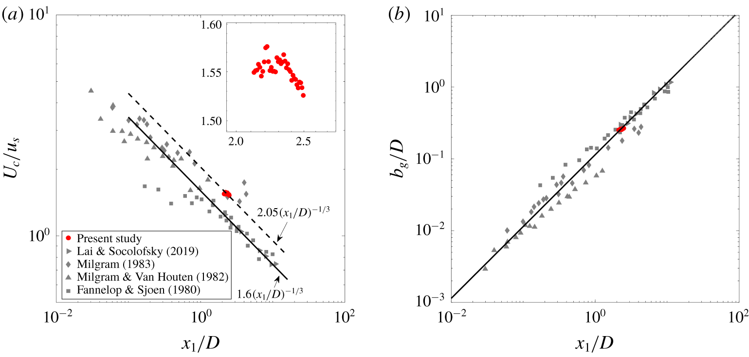
Figure 7. Comparison of (a) mean centreline velocity,  $U_{c}$, and (b) Gaussian plume radius, $b_{g}$, between a particle plume (current study) and bubble plume (published literature).

Figure 8. Radial profiles of non-dimensional (a)  $\langle U_{2}\rangle /U_{c}$ and (b) $\langle U_{3}\rangle /U_{c}$ at various axial locations ( $x_{1}/d_{0}$) indicated by the colourbar.
Profiles of mean radial ( $\langle U_{2}\rangle$) and out-of-plane ( $\langle U_{3}\rangle$) velocities at various axial locations are shown in figures 8(a) and 8(b), respectively. The mean radial velocity exhibits typical jet/plume behaviour: within the plume radius ( $|x_{2}/b_{g}|\,<\,1$) the interstitial fluid flows away from the centreline, whereas outside the plume radius ( $|x_{2}/b_{g}|>1$) the surrounding fluid is entrained into the plume. The mean out-of-plane velocity should be zero by design (swirling motions are not introduced by the particle feeder) but it shows some variations and asymmetry far from the plume axis. The solid line in figure 8(a) is a nonlinear least squares fit to a shape function,
 $$\begin{eqnarray}\frac{\langle U_{2}\rangle }{U_{c}}=-\frac{\unicode[STIX]{x1D6FC}}{\unicode[STIX]{x1D702}}\left((1-\text{e}^{-\unicode[STIX]{x1D702}^{2}})-\frac{\unicode[STIX]{x1D6FD}}{\unicode[STIX]{x1D6FC}}\unicode[STIX]{x1D702}^{2}\text{e}^{-\unicode[STIX]{x1D702}^{2}}\right).\end{eqnarray}$$
 Here,  $\unicode[STIX]{x1D702}=x_{2}/b_{g}$. The shape function in (3.1) is obtained from the radial integration of the continuity equation written in a cylindrical coordinate system after adopting the entrainment hypothesis for jets/plumes and the Gaussian-profile assumption for $\langle U_{1}\rangle$ (Papanicolaou & List Reference Papanicolaou and List1988; Lee & Chu Reference Lee and Chu2003). Herein, the entrainment coefficient, $\unicode[STIX]{x1D6FC}$=0.07 is computed as a fitting parameter in (3.1). The spreading versus entrainment ratio, $\unicode[STIX]{x1D6FD}/\unicode[STIX]{x1D6FC}$, has been measured as 2 for pure jets (Lee & Chu Reference Lee and Chu2003), and 1.2 for bubble plumes (Lai & Socolofsky Reference Lai and Socolofsky2019). Our results show $\unicode[STIX]{x1D6FD}/\unicode[STIX]{x1D6FC}=0.114/0.07=1.63$, situating the particle-laden plume between pure jets and bubble plumes.
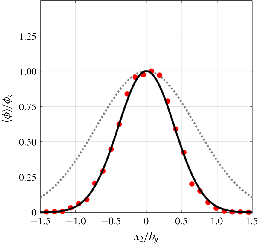
Figure 9. Normalized distribution of particle number density across the plume averaged along  $x_{1}$. The solid line is a Gaussian fit to the measured data, and the dotted line is the Gaussian fit to mean axial fluid velocity ( $\langle U_{1}\rangle /U_{c}$) from figure 6. The particle half-width, $b_{\unicode[STIX]{x1D719}}=0.56b_{g}$.
We compute particle number density by counting the particles across each sample (detection method described in § 2.3.2). The normalized distribution of particle number density  $\unicode[STIX]{x1D719}$ across the radius of the plume is shown in figure 9. Here, $\langle \unicode[STIX]{x1D719}\rangle$ signifies the probability of finding a particle in the specified radial location, and $\unicode[STIX]{x1D719}_{c}$ is the centreline value, which measures as 0.11 at all axial locations. The distribution of $\unicode[STIX]{x1D719}$ allows us to fit a Gaussian profile and measure the half-width ( $b_{\unicode[STIX]{x1D719}}$), which we use to designate the ‘particle core’ from here onward. The axially averaged $b_{\unicode[STIX]{x1D719}}$ obtained from the particle concentration profiles, when normalized by the axially averaged $b_{g}$, shows that $b_{\unicode[STIX]{x1D719}}/b_{g}=0.56$. This ratio for the bubble plume in Lai & Socolofsky (Reference Lai and Socolofsky2019) was not measured, but in earlier studies of bubble plumes, e.g. Milgram (Reference Milgram1983), reported values of $b_{\unicode[STIX]{x1D719}}/b_{g}$ are in the range of 0.8–0.9. This value is somewhat higher than our value, implying that solid particles spread less rapidly than bubbles. This may be due to the fact that rising bubbles exhibit swirling motions and experience significant lateral lift force when compared to particles (Lai & Socolofsky Reference Lai and Socolofsky2019). In addition, LES for a range of monodispersed and polydispersed bubble plumes in Fraga & Stoesser (Reference Fraga and Stoesser2016) show that the ratio $b_{\unicode[STIX]{x1D719}}/b_{g}$ is very sensitive to the size distribution of bubbles across the plume. They showed that the size distribution across the plume resembles a reverse-Gaussian profile with larger bubbles populating away from the centreline. This reveals the complexity related to clearly defining a bubble-core which depends on the distribution of the number density as well as bubble size across the plume. A future investigation on bubble plumes examining the relationship between polydispersity and turbulence characteristics will help to better explain the above differences between the particle and bubble plumes.
The dynamic length scale  $D$ in the above formulation was derived by Bombardelli et al. (Reference Bombardelli, Buscaglia, Rehmann, Rincon and Garcia2007), wherein the authors started with the governing equations (continuity and momentum) of the air–water mixture, which were derived from a two-fluid approach (Buscaglia, Bombardelli & Garcia Reference Buscaglia, Bombardelli and Garcia2002). The mixture was assumed to have low air void fractions, to be incompressible and the Boussinesq approximation for small density differences to be valid. For bubble plumes having air void fractions of the order of a few per cent, this is equivalent to the usual Boussinesq approximation applied to single-phase water flows like seawater. The parameter $D$ was then obtained from the non-dimensional momentum equation by requiring a balance between inertia and buoyancy.

Figure 10. Comparison of standardized p.d.f. of (a) axial,  $u_{1}/u_{1,rms}$; (b) radial, $u_{2}/u_{2,rms}$, and out-of-plane, $u_{3}/u_{3,rms}$, velocity fluctuations at the centreline of a particle plume (present data) and a bubble plume (Lai & Socolofsky Reference Lai and Socolofsky2019). In (a), positive values indicate upward-moving fluid in the case of bubble plume and downward-moving fluid in the case of particle plume.
To apply the above formulation to particle-laden plumes, care must be taken to ensure that the Boussinesq approximation remains valid in the mean flow, and thus, imposing restrictions on the type of particles that can be considered. In our study, the specific gravity of Teflon particles relative to water is 2.15. The mixture density equation gives a density difference  $\unicode[STIX]{x1D719}(\unicode[STIX]{x1D70C}_{s}-\unicode[STIX]{x1D70C}_{w})=\unicode[STIX]{x1D719}(2.15-1)\unicode[STIX]{x1D70C}_{w}=1.15\unicode[STIX]{x1D719}\unicode[STIX]{x1D70C}_{w}$. The maximum solid fraction, $\unicode[STIX]{x1D719}$, occurs at the plume centreline and is approximately 10 %. This gives a density difference of approximately 10 %, $(\unicode[STIX]{x1D70C}_{m}-\unicode[STIX]{x1D70C}_{w})/\unicode[STIX]{x1D70C}_{w}\approx 0.1$. This 10 % is a little bit on the high side but is not unreasonable. The possible mild violation of the Boussinesq approximation at the plume centreline should not invalidate the formulation that seeks to predict the overall, plume-scale dynamics.
3.2 Fluctuating flow characteristics
In this section, we examine the nature of the fluctuating components of velocity ( $u_{i}=U_{i}-\langle U_{i}\rangle$, $u_{i,rms}=\sqrt{\langle u_{i}^{2}\rangle }$). The normalized p.d.f. of $u_{i}$ at the plume centreline is shown in figure 10. The respective p.d.f. for a bubble plume (Lai & Socolofsky Reference Lai and Socolofsky2019) is also included in each plot for comparison. Interestingly, the distribution of the axial velocity fluctuations is negatively skewed for a particle plume, such that axial fluctuations opposite to the direction of particle motion are more common than those along the direction of particle motion. This behaviour is strikingly opposite to what is seen in bubble plumes and homogeneous bubble swarms (Riboux, Risso & Legendre Reference Riboux, Risso and Legendre2010; Prakash et al. Reference Prakash, Mercado, Wijngaarden, Mancilla, Tagawa, Lohse and Sun2016; Lai & Socolofsky Reference Lai and Socolofsky2019), for which the axial velocity fluctuations moving in the direction of bubble motion are more common than those moving in the opposite direction. Another way to see this effect is that the mode of the distribution is slightly positive for the particle plume, while it is slightly negative for a bubble plume (see figure 10a). One implication of this contrasting result is that the turbulence in a multiphase plume is sensitive to the direction of the plume with respect to gravity; particle plumes are not a simple reversal of bubble plumes. One implication of this contrasting result could be that the fluid flow in a multiphase plume is non-Boussinesq and is sensitive to the direction of the plume with respect to gravity. The cause of this difference could be the deformability of bubbles, the different density contrast between the two phases (2 : 1 for a particle plume and 0.001 : 1 for a bubble plume), or the different inertia between a bubble and a particle. All of these factors cause structural differences in the wake of a particle compared to that of a bubble and thus the role of role of added mass in these two flows. A future study comparing the wake-to-wake interaction in a particle plume with that in a bubble plume will help clarifying these differences between the two flows.
The p.d.f.s of radial and out-of-plane velocity fluctuations are symmetric about their means (figure 10b), and closely follow a Gaussian curve. We do not observe the prominent signatures of intermittency in the cross-stream components typically observed in bubble plumes and bubble swarms (Prakash et al. Reference Prakash, Mercado, Wijngaarden, Mancilla, Tagawa, Lohse and Sun2016; Lai & Socolofsky Reference Lai and Socolofsky2019).
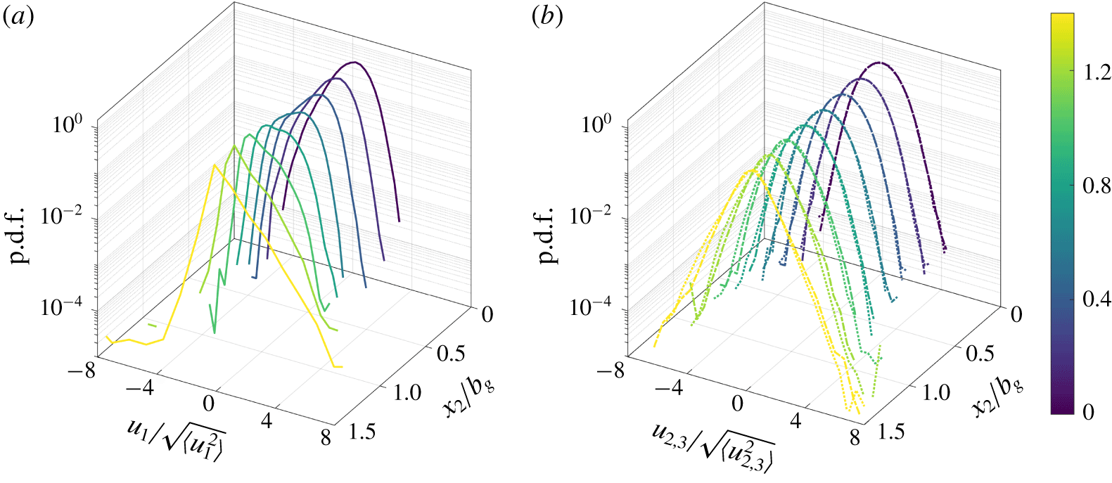
Figure 11. Standardized p.d.f. of (a) axial,  $u_{1}/u_{1,rms}$; (b) radial, $u_{2}/u_{2,rms}$; and out-of-plane, $u_{3}/u_{3,rms}$ at various locations across a particle plume. The colourbar indicates the various radial locations ( $x_{2}/b_{g}$).
In figure 11, we further examine the velocity fluctuations across the plume at different radial locations ( $x_{2}/b_{g}$). For this purpose, we sort the data into eight equal bins ( $\text{bin width}=0.16b_{g}$) for $x_{2}\geqslant 0$ after checking that the choice of bin width does not change the results. Across the plume, the radial, $u_{2}$, and out-of-plane, $u_{3}$, velocity fluctuations are symmetric with nearly zero skewness (see figure 11b). The axial velocity fluctuations, $u_{1}$, switch from negatively skewed at the centreline (as discussed earlier) to positively skewed outside the half-radius ( $x_{2}>0.5b_{g}$) of the plume. These characteristics are better captured in the statistical moments (r.m.s., skewness and kurtosis) as shown in figure 12. Figure 12(b) shows that the change of sign in $S(u_{1})$ occurs at three-quarters of the plume width $b_{g}$, which also coincides with the maximum $u_{1,rms}$ (see figure 12a). Both $u_{2,rms}$ and $u_{3,rms}$ show their maximum at the centreline, and are consistently smaller than $u_{1,rms}$. The radial variation of kurtosis $K(u_{i})$ in figure 12(c) captures the increasing flatness of each distribution outside the plume half-radius.

Figure 12. Higher-order statistics: (a) standard deviation; (b) skewness; and (c) kurtosis of the three components of velocity fluctuations across a particle plume.
3.3 Reynolds stresses

Figure 13. Radial profiles of normalized (a) turbulent normal stresses:  $\langle u_{1}^{2}\rangle /U_{c}^{2}$, (○); $\langle u_{2}^{2}\rangle /U_{c}^{2}$, (▫); and $\langle u_{3}^{2}\rangle /U_{c}^{2}$, (▵); (b) normalized turbulent shear stress $\langle u_{1}u_{2}\rangle /U_{c}^{2}$; and (c) normalized turbulent kinetic energy ( $k/U_{c}^{2}$) at various axial locations. The colourbars show the normalized axial locations ( $x_{1}/d_{0}$) indicated by the colourbar.
The Reynolds stresses across the plume are reported at all measured axial locations in figures 13(a) (normal stresses) and 13(b) (shear stress in the measurement plane). The turbulent kinetic energy ( $k$) based on 13(a) is shown separately in figure 13(c). A nonlinear least squares fit of the data to a shape-preserving function (see appendix A) captures well each profile (see fitted lines in figure 13). Results show that the turbulent kinetic energy is primarily dominated by the axial velocity fluctuations, and that it increases from the plume centreline to its maximum value near the edge of the plume ( $x_{2}\approx 0.75b_{g}$). The maximum TKE located at $x_{2}/b_{g}=0.75$ is approximately 44 % of $U_{c}^{2}$ and is approximately 1.5 times the TKE at the plume centre. The in-plane shear stress, $\langle u_{1}u_{2}\rangle /U_{c}^{2}$, follows a trend similar to that of a turbulent jet and increases from zero at the centreline to a maximum located near $x_{2}/b_{g}=0.75$ (see figure 13b). The location of maximum shear is consistent with that of $\langle u_{1}^{2}\rangle /U_{c}^{2}$, suggesting that the shear stress is dominated by the axial fluctuations $u_{1}$.
In figure 14, we compare the in-plane turbulent intensities normalized by the local mean axial velocity, ( $\sqrt{\langle u_{1}^{2}\rangle }/\langle U_{1}\rangle$), with two earlier studies on bubble plumes (Duncan, Seol & Socolofsky Reference Duncan, Seol and Socolofsky2009; Lai & Socolofsky Reference Lai and Socolofsky2019). For this comparison, we use the shape functions (solid and dashed lines in figure 13(a)). The present data and the data from Duncan et al. (Reference Duncan, Seol and Socolofsky2009) show reasonably similar trends with unbounded growth away from the centreline as $\langle U_{1}\rangle$ approaches zero asymptotically outside the plume. The results from Lai & Socolofsky (Reference Lai and Socolofsky2019) show somewhat higher turbulent intensity inside the plume core. Also, the growth in their normalized turbulent intensities is not unbounded. Lai & Socolofsky (Reference Lai and Socolofsky2019) attribute this deviation to finite $\langle U_{1}\rangle$ outside of the plume caused by large recirculation cells caused by the tank walls; also shown in the LES simulations in Fraga & Stoesser (Reference Fraga and Stoesser2016). This created a non-zero upward mean flow and so the normalized stresses do not attain infinitely large values at the plume edges in their study. The centreline turbulent intensities for the present data are 18 %, 11 % and 9 % for $u_{1}$, $u_{2}$ and $u_{3}$, respectively. The axial turbulent intensity ( $\sqrt{\langle u_{1}^{2}\rangle }$) at the centreline for a bubble plume (Lai & Socolofsky Reference Lai and Socolofsky2019) is also approximately twice the other two normal intensities ( $\sqrt{\langle u_{2,3}^{2}\rangle }$), suggesting stronger anisotropy in multiphase plumes when compared to a single-phase jets/plumes in which the ratio $\sqrt{\langle u_{1}^{2}\rangle /\langle u_{2,3}^{2}\rangle }$ is approximately 1.4 (Wang & Law Reference Wang and Law2002).

Figure 14. (a) Axial and (b) radial turbulence intensities normalized by the local mean axial velocity  $\langle U_{1}\rangle$.
3.4 Conservation of kinematic momentum flux of the plume
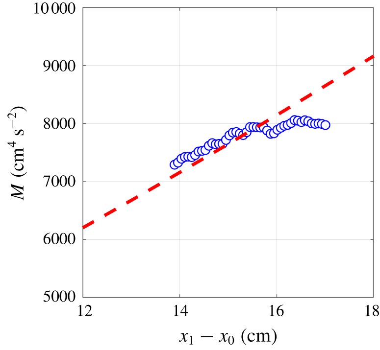
Figure 15. Variation of total kinematic momentum flux of the induced liquid flow in a particle plume along the axial direction. The dashed line shows a model prediction from (3.2).
Using the method in Lai & Socolofsky (Reference Lai and Socolofsky2019), we assess the conservation of the total kinematic momentum flux,  $M=\langle M\rangle +M_{t}$, of the induced liquid flow in our particle plume in figure 15. Here, the momentum flux contributed by the mean flow is $\langle M\rangle =2\unicode[STIX]{x03C0}\int _{0}^{\infty }x_{2}U_{1}^{2}\,\text{d}x_{2}$. The momentum flux carried by the turbulence fluctuations is computed as $M_{t}=2\unicode[STIX]{x03C0}\int _{0}^{\infty }x_{2}(\langle u_{1}^{2}\rangle -0.5(\langle u_{2}^{2}\rangle +\langle u_{3}^{2}\rangle ))\,\text{d}x_{2}$. The results are compared to the analytical expression for $M(x_{1})$ for pure vertical plumes (Lee & Chu Reference Lee and Chu2003),
 $$\begin{eqnarray}M(x_{1})=(3\sqrt{2\unicode[STIX]{x03C0}}\unicode[STIX]{x1D6FD}F_{0}/4)^{2/3}(x_{1}-x_{0})^{4/3}.\end{eqnarray}$$
 Here,  $x_{0}=-5.6d_{0}$ is the virtual origin of the plume and $F_{0}=Q_{0}g$ is the buoyancy flux of the particles. Our results show reasonably good agreement with this model, suggesting that the particle plume obeys the scaling law $M\sim x_{1}^{4/3}$, which is consistent with buoyancy-driven plumes. Some deviation from this power law is observed beyond axial location $x_{1}-x_{0}>16~\text{cm}$ where the value of $\langle M\rangle$ becomes almost flat. This is attributed to PIV measurement uncertainty near the edge of our measurement window. The total momentum flux is primarily contributed by the momentum flux due to the mean flow $\langle M\rangle$. The remaining contribution comes from $M_{t}$, and it is customary to quantify the contribution by the local momentum amplification factor $\unicode[STIX]{x1D6FE}=M/\langle M\rangle$. For our particle plume, $\unicode[STIX]{x1D6FE}$ is 1.2, averaged across all axial measurements. This result shows that $\unicode[STIX]{x1D6FE}$ for a particle plume is larger than that for a single-phase jet/plume ( $\unicode[STIX]{x1D6FE}=1.07{-}1.09$ (Wang & Law Reference Wang and Law2002)) and smaller than a bubble plume ( $\unicode[STIX]{x1D6FE}=1.4{-}1.6$ (Lai & Socolofsky Reference Lai and Socolofsky2019)).
3.5 Velocity triple correlation and turbulent transport
Because the p.d.f. of axial velocity fluctuations in a particle and a bubble plume are oppositely skewed (see figure 10a), some interesting differences between the two flows can be identified in terms of the velocity triple-correlation terms. These terms contribute to the transport of turbulent kinetic energy and thus are important in the TKE budget (§ 3.7). The radial profiles of the triple correlation of in-plane velocity fluctuations normalized by  $U_{c}^{3}$ are shown in figure 16. To compare the trends we also show the respective profiles for a single-phase jet (Darisse et al. Reference Darisse, Lemay and Benaïssa2012) and a bubble plume (Lai & Socolofsky Reference Lai and Socolofsky2019). The profiles extracted from the two references are multiplied by a factor for visual comparison (see legends in figure 16).
Other than  $\langle u_{1}^{3}\rangle$, all triple-correlation profiles for the particle plume show trends similar to a turbulent single-phase jet. The triple-correlation profiles of the first two terms ( $\langle u_{1}^{3}\rangle /U_{c}^{3}$ and $\langle u_{1}u_{2}^{2}\rangle /U_{c}^{3}$) for the bubble plume in Lai & Socolofsky (Reference Lai and Socolofsky2019) are significantly different from the single-phase jet and our particle plume, and they show 10–20 times larger magnitude compared to our particle plume results (see figure 16a,b). The bubble plume shows a positive $\langle u_{1}^{3}\rangle$ near the centreline as opposed to the negative $\langle u_{1}^{3}\rangle$ observed near the core of the particle plume, due to the opposite skewness of their $u_{1}$ distributions discussed earlier (see figure 10a).
Based on the triple-correlation terms computed above, we estimate the axial and radial transport of  $k$ in figures 17(a) and 17(b), respectively. Since the TKE in the particle plume is primarily contributed by the axial stress, $\langle u_{1}^{2}\rangle$, these two profiles are nearly identical to those in figure 16(a,c). These profiles are fitted to two shape functions (see appendix A) and are shown as solid lines in figures 17(a) and 17(b), respectively. We use them for estimating the TKE budget in § 3.7.

Figure 16. Normalized radial profiles of triple correlations (a,b) axial transport ( $\langle u_{1}u_{i}^{2}\rangle$) and (c,d) radial transport ( $\langle u_{2}u_{i}^{2}\rangle$) of in-plane components of turbulent kinetic energy in a particle plume at various axial locations ( $x_{1}/d_{0}$) indicated by the colourbar compared with a single-phase jet (Darisse et al. Reference Darisse, Lemay and Benaïssa2012) and a bubble plume (Lai & Socolofsky Reference Lai and Socolofsky2019).
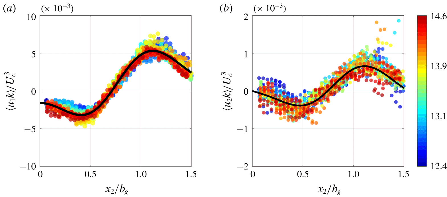
Figure 17. Radial profiles of non-dimensional (a) axial ( $\langle u_{1}k\rangle /U_{c}^{3}$) and (b) radial ( $\langle u_{2}k\rangle /U_{c}^{3}$) transport of turbulent kinetic energy at various axial locations ( $x_{1}/d_{0}$) indicated by the colourbar.
3.6 Mean square gradients of velocity fluctuations
To test the conditions of local isotropy and local axisymmetry (George & Hussein Reference George and Hussein1991), we compute the in-plane derivatives of all three components of velocity fluctuations employing the second-order-accurate central difference scheme. Table 3 and figure 18 show the second moments of axial ( $\unicode[STIX]{x2202}/\unicode[STIX]{x2202}x_{1}$) and radial ( $\unicode[STIX]{x2202}/\unicode[STIX]{x2202}x_{2}$) derivatives of all three components of velocity. These moments clearly do not satisfy the conditions of local isotropy (e.g. $\langle (\unicode[STIX]{x2202}u_{1}/\unicode[STIX]{x2202}x_{1})^{2}\rangle \neq \langle (\unicode[STIX]{x2202}u_{2}/\unicode[STIX]{x2202}x_{2})^{2}\rangle$ and $\langle (\unicode[STIX]{x2202}u_{1}/\unicode[STIX]{x2202}x_{2})^{2}\rangle \neq 2\langle (\unicode[STIX]{x2202}u_{1}/\unicode[STIX]{x2202}x_{1})^{2}\rangle$) nor of local axisymmetry (e.g. $\langle (\unicode[STIX]{x2202}u_{3}/\unicode[STIX]{x2202}x_{1})^{2}\rangle \neq \langle (\unicode[STIX]{x2202}u_{2}/\unicode[STIX]{x2202}x_{1})^{2}\rangle$).
Table 3. The second moment of the six available components of the velocity gradient tensor averaged axially and radially. The quantities within the bracket indicate the 95 % uncertainty bounds obtained with the bootstrap method.
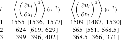
The violation of local axisymmetry was also observed for bubble plumes (Lai & Socolofsky Reference Lai and Socolofsky2019), suggesting that this is a common characteristic of multiphase plume turbulence contrary to single-phase jets.

Figure 18. Radial profiles of non-dimensional (a) axial ( $\langle u_{1}k\rangle /U_{c}^{3}$) and (b) radial ( $\langle u_{2}k\rangle /U_{c}^{3}$) transport of turbulent kinetic energy at various axial locations ( $x_{1}/d_{0}$) indicated by the colourbar.
Computing the true viscous dissipation rate (stress power) requires all nine components of the velocity gradient tensor and each component has to be adequately resolved, which is not easy to achieve experimentally. Instead, we compute the pseudo-dissipation rate  $\langle \unicode[STIX]{x1D716}\rangle$ (Pope Reference Pope2000),
 $$\begin{eqnarray}\displaystyle \langle \unicode[STIX]{x1D716}\rangle & = & \displaystyle \unicode[STIX]{x1D708}\left[\left\langle \left(\frac{\unicode[STIX]{x2202}u_{1}}{\unicode[STIX]{x2202}x_{1}}\right)^{2}\right\rangle +\left\langle \left(\frac{\unicode[STIX]{x2202}u_{1}}{\unicode[STIX]{x2202}x_{2}}\right)^{2}\right\rangle +\left\langle \left(\frac{\unicode[STIX]{x2202}u_{1}}{\unicode[STIX]{x2202}x_{3}}\right)^{2}\right\rangle \right.\nonumber\\ \displaystyle & & \displaystyle +\,\left\langle \left(\frac{\unicode[STIX]{x2202}u_{2}}{\unicode[STIX]{x2202}x_{1}}\right)^{2}\right\rangle +\left\langle \left(\frac{\unicode[STIX]{x2202}u_{2}}{\unicode[STIX]{x2202}x_{2}}\right)^{2}\right\rangle +\left\langle \left(\frac{\unicode[STIX]{x2202}u_{2}}{\unicode[STIX]{x2202}x_{3}}\right)^{2}\right\rangle \nonumber\\ \displaystyle & & \displaystyle +\left.\left\langle \left(\frac{\unicode[STIX]{x2202}u_{3}}{\unicode[STIX]{x2202}x_{1}}\right)^{2}\right\rangle +\left\langle \left(\frac{\unicode[STIX]{x2202}u_{3}}{\unicode[STIX]{x2202}x_{2}}\right)^{2}\right\rangle +\left\langle \left(\frac{\unicode[STIX]{x2202}u_{3}}{\unicode[STIX]{x2202}x_{3}}\right)^{2}\right\rangle \right].\end{eqnarray}$$
 Here,  $\unicode[STIX]{x1D708}=1.02\times 10^{-6}~\text{m}^{2}~\text{s}^{-1}$ is the kinematic viscosity of saline water at $23\,^{\circ }\text{C}$. In our calculations all but the three out-of-plane derivative terms in (3.3) are computed directly from our SPIV data, and the missing out-of-plane mean-square derivatives ( $\langle (\unicode[STIX]{x2202}u_{i}/\unicode[STIX]{x2202}x_{3})^{2}\rangle$) are replaced by $\langle (\unicode[STIX]{x2202}u_{i}/\unicode[STIX]{x2202}x_{2})^{2}\rangle$. The mean pseudo-dissipation rate $\langle \unicode[STIX]{x1D716}\rangle$ across the plume is shown for various axial locations in figure 19.

Figure 19. Radial profiles of non-dimensional mean dissipation rate at various axial locations ( $x_{1}/d_{0}$) indicated by the colourbar.
To assess the accuracy in the dissipation calculation, we adopt a method based on conservation of total kinetic energy for multiphase plume in a Lagrangian framework as outlined in Lai & Socolofsky (Reference Lai and Socolofsky2019). In essence, this method estimates the balance of the total kinetic energy as production minus dissipation
 $$\begin{eqnarray}\iiint _{V}\frac{D}{Dt}(\langle K\rangle +\langle k\rangle )\,\text{d}V=-f_{c}\iiint _{V}\langle \unicode[STIX]{x1D716}\rangle \,\text{d}V+\iiint _{V}\frac{\unicode[STIX]{x0394}\unicode[STIX]{x1D70C}}{\unicode[STIX]{x1D70C}}\langle U_{1}\rangle g\,\text{d}V,\end{eqnarray}$$
 and calculates the correction factor  $f_{c}$ to balance the two sides. The mean kinetic energy, $\langle K\rangle \approx \langle U_{1}\rangle ^{2}/2$ because $U_{1}\gg U_{2},U_{3}$. This equation can be simplified in the cylindrical coordinate system ( $r,\unicode[STIX]{x1D703},z$) by invoking steady state as follows. The left-hand side of the equation is computed using the shape functions of the mean radial profiles for $\langle U_{1}\rangle$ and $\langle k\rangle$ (see §§ 3.1 and 3.2). The first term on the right-hand side is obtained by using $\langle \unicode[STIX]{x1D716}\rangle$ at multiple axial locations. The last term in (3.4) refers to the kinetic energy production due to the particle buoyancy flux and equals $CF_{0}\unicode[STIX]{x0394}x_{1}$, where the prefactor $C=1+\unicode[STIX]{x1D706}^{2}/\unicode[STIX]{x03C0}\unicode[STIX]{x1D706}^{2}\sqrt{4/\unicode[STIX]{x1D6FE}}\int _{0}^{\infty }2\unicode[STIX]{x03C0}\unicode[STIX]{x1D702}\text{e}^{-(2\unicode[STIX]{x1D706}^{2}+1/\unicode[STIX]{x1D706}^{2})\unicode[STIX]{x1D702}^{2}}\,\text{d}\unicode[STIX]{x1D702}$ depends on $\unicode[STIX]{x1D706}=\langle b_{\unicode[STIX]{x1D719}}\rangle /\langle b_{g}\rangle$ and the momentum amplification factor $\unicode[STIX]{x1D6FE}$. Based on $\unicode[STIX]{x1D706}=0.6$ and $\unicode[STIX]{x1D6FE}=1.2$, we obtain $C=1.44$. The simplified equation for a volume bounded by two axial locations $x_{1}$ and $x_{2}$ is written as
 $$\begin{eqnarray}[(0.5I_{1}+I_{2})(b_{g}^{2}U_{c}^{3})]_{x_{1}}^{x_{2}}=f_{c}\int _{z_{1}}^{z_{2}}I_{3}b_{g}U_{c}^{3}\,\text{d}x+1.44F_{0}\unicode[STIX]{x0394}x_{1}.\end{eqnarray}$$
 Here,  $I_{1}$, $I_{2}$ and $I_{3}$ are the axisymmetric surface integrals ( $2\unicode[STIX]{x03C0}\int _{0}^{\infty }(.)r\,\text{d}r$) of the respective terms inside the volume integral in (3.4) (summarized in table 4).
Table 4. Simplified similarity expressions and values of various integrals used in (3.5). The shape functions  $F_{4}(\unicode[STIX]{x1D702})$ and $F_{5}(\unicode[STIX]{x1D702})$ are summarized in appendix A.
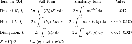
We test the balance of (3.5) at multiple axial locations separated by  $1.5b_{g}$ and have found $f_{c}$ to vary between 2.8 and 5.1 with a mean value of 4.0. This method estimates the amount by which $\langle \unicode[STIX]{x1D716}\rangle$ is underestimated by our evaluation of (3.6), but it is unable to correct $\langle \unicode[STIX]{x1D716}\rangle$ locally along the radius of the plume. Given such limitation, $\langle \unicode[STIX]{x1D716}\rangle$ presented here must be interpreted as order of magnitude estimates. We use the corrected dissipation profile only for a qualitative assessment of the TKE budget discussed in the following section.
3.7 Turbulent kinetic energy budget
In the cylindrical coordinate system, the time-averaged transport equation for  $k$ of an axisymmetric, steady, turbulent plume without swirl is (Kataoka & Serizawa Reference Kataoka and Serizawa1989)
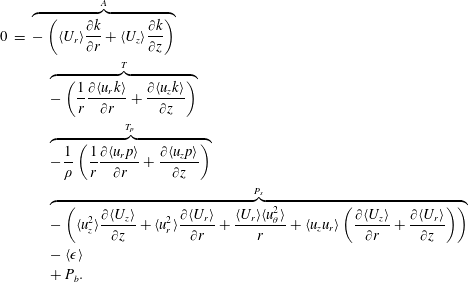 $$\begin{eqnarray}\displaystyle 0 & = & \displaystyle \overbrace{-\left(\langle U_{r}\rangle \frac{\unicode[STIX]{x2202}k}{\unicode[STIX]{x2202}r}+\langle U_{z}\rangle \frac{\unicode[STIX]{x2202}k}{\unicode[STIX]{x2202}z}\right)}^{A}\nonumber\\ \displaystyle & & \displaystyle \quad \overbrace{-\left(\frac{1}{r}\frac{\unicode[STIX]{x2202}\langle u_{r}k\rangle }{\unicode[STIX]{x2202}r}+\frac{\unicode[STIX]{x2202}\langle u_{z}k\rangle }{\unicode[STIX]{x2202}z}\right)}^{T}\nonumber\\ \displaystyle & & \displaystyle \quad \overbrace{-\frac{1}{\unicode[STIX]{x1D70C}}\left(\frac{1}{r}\frac{\unicode[STIX]{x2202}\langle u_{r}p\rangle }{\unicode[STIX]{x2202}r}+\frac{\unicode[STIX]{x2202}\langle u_{z}p\rangle }{\unicode[STIX]{x2202}z}\right)}^{T_{p}}\nonumber\\ \displaystyle & & \displaystyle \quad \overbrace{-\left(\langle u_{z}^{2}\rangle \frac{\unicode[STIX]{x2202}\langle U_{z}\rangle }{\unicode[STIX]{x2202}z}+\langle u_{r}^{2}\rangle \frac{\unicode[STIX]{x2202}\langle U_{r}\rangle }{\unicode[STIX]{x2202}r}+\frac{\langle U_{r}\rangle \langle u_{\unicode[STIX]{x1D703}}^{2}\rangle }{r}+\langle u_{z}u_{r}\rangle \left(\frac{\unicode[STIX]{x2202}\langle U_{z}\rangle }{\unicode[STIX]{x2202}r}+\frac{\unicode[STIX]{x2202}\langle U_{r}\rangle }{\unicode[STIX]{x2202}z}\right)\right)}^{P_{s}}\nonumber\\ \displaystyle & & \displaystyle \quad -\langle \unicode[STIX]{x1D716}\rangle \nonumber\\ \displaystyle & & \displaystyle \quad +P_{b}.\end{eqnarray}$$
 In addition to the terms already present in single-phase jets/plumes ( $A$, advection; $P_{s}$, shear-production; $T$, turbulent transport; and $T_{p}$, pressure transport), a multiphase plume has another source term ( $P_{b}$) that represents the interfacial energy transfer at the boundaries between the dispersed phase and the surrounding fluid. Obtaining the complete TKE budget for a particle plume is challenging for multiple reasons. First, it is difficult to accurately measure experimentally the mean dissipation rate $\langle \unicode[STIX]{x1D716}\rangle$ because of the under-resolved velocity gradients (as seen in § 3.6). Second, there is no existing model for pressure–velocity correlation in multiphase flow turbulence, and therefore the pressure transport term ( $T_{p}$) requires an assumption. Finally, the interfacial energy transfer ( $P_{b}$) is the most complex and inaccessible term, and it requires the local distribution of particles and their relative velocity with the surrounding fluid (Santarelli, Rouseel & Frohlich Reference Santarelli and Rouseel2016). In an ideal scenario with all other terms measured correctly, the term $P_{b}$ can be sought as the closing term of (3.6), such that $P_{b}=\langle \unicode[STIX]{x1D716}\rangle -(A+P_{s}+T+T_{p})$. We will use this method to estimate $P_{b}$ from our data.

Figure 20. Various terms in the turbulent kinetic energy budget for (a) a particle plume and (b) a bubble plume reproduced from Lai & Socolofsky (Reference Lai and Socolofsky2019). The error band in each term (shown up to the extent of measurement window) represents uncertainty in computing the term.
We directly compute  $A$,
$A$,  $P_{s}$ and $T$ from our experimental data. The expressions for these in terms of similarity variables are summarized in appendix B. Each plot contains an error band corresponding to the 95 % confidence interval in the constituent fits. Each uncertainty band is computed via the rule of uncertainty propagation described in Charonko & Prestridge (Reference Charonko and Prestridge2017). The pressure transport term, $T_{p}$, not directly available from experiment, is replaced by Lumley’s model $T_{p}=-2/5T$, widely used for single-phase turbulence (Lumley Reference Lumley1978). These four terms and the mean dissipation rate ( $\langle \unicode[STIX]{x1D716}\rangle$) multiplied by the correction factor $f_{c}=4$ are shown in figure 20(a). The remaining terms of the balance equation are the interfacial energy transfer ( $P_{b}$) from particles to fluid and out-of-balance experimental error (known as OOBE). The budget terms for a bubble plume from Lai & Socolofsky (Reference Lai and Socolofsky2019) are reproduced in figure 20(b) for comparison. Each budget term is normalized by $U_{c}^{3}/b_{g}$; the order of magnitude difference in the two budgets arises because of the difference in the downstream measurement locations with respect to the source, leading to the differences in $U_{c}$ and $b_{g}$ (see figure 7a,b). Below we discuss the comparison of the TKE budget for the two multiphase plumes in light of previous experiments on a single-phase jet (Lai & Socolofsky Reference Lai and Socolofsky2018) and a variable-density single-phase (VDSP) jet (Charonko & Prestridge Reference Charonko and Prestridge2017). The qualitative summary of this comparison is provided in table 5.
The shape of the advection ( $A$) profiles are very similar across all four plumes with a positive central lobe inside the plume core. The shear production term ( $P_{s}$) in the particle plume increases from zero at the centreline to a dominant peak at approximately $r/b_{g}=0.65$ near the edge of the plume. This behaviour strongly resembles a single-phase jet both in shape and relative magnitude. The $P_{s}$ profile in the VDSP jet also matches this trend, except that a negative $P_{s}$ is observed at the jet centreline. By contrast, the bubble plume shows almost negligible $P_{s}$ across the radius of the plume. The turbulent transport term ( $T$) in the particle plume exhibits a positive peak near the centreline and a negative lobe near the edge of the plume. The bubble plume and the VDSP jet are similar, but with a larger peak in the former. The single-phase jet does not match the others, i.e. near the centreline the turbulent transport is consistently observed to be negative or marginally positive (Darisse, Lemay & Benaïssa Reference Darisse, Lemay and Benaïssa2015).
Table 5. Qualitative comparison summary of three TKE budget terms in our particle plume and those in a bubble plume (Lai & Socolofsky Reference Lai and Socolofsky2019), a single-phase jet (Darisse et al. Reference Darisse, Lemay and Benaïssa2015; Lai & Socolofsky Reference Lai and Socolofsky2018) and a VDSP jet (Charonko & Prestridge Reference Charonko and Prestridge2017).
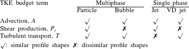
Because the energy production at the two-phase boundaries,  $P_{b}$, is computed indirectly, the peak location in $P_{b}$ is sensitive to the experimental error in $\langle \unicode[STIX]{x1D716}\rangle$. Despite this limitation, it is worth noting that in both particle and bubble plumes, the sum ( $A+T+P_{s}+T_{p}$) is significantly smaller than the mean dissipation rate outside the plume core ( $r>0.5b_{g}$). This results in the TKE budget being an approximate balance between $P_{b}$ and $\langle \unicode[STIX]{x1D716}\rangle$ lending further credibility to our results.
3.8 Two-point correlation and energy spectra
We obtain the two-point statistics from the spatial autocorrelation function  $R_{11}$ computed along the axial measurements of axial velocity fluctuations, $u_{1}$. Figure 21 shows $R_{11}$ inside the plume core ( $x_{2}/b_{g}<0.5$) at various radial locations (shaded circles) and their mean $\bar{R}_{11}$ (red circles). The horizontal axis is normalized by the particle diameter $d_{p}$. We estimate the Taylor microscale ( $\unicode[STIX]{x1D706}_{f}$) of this flow by fitting an osculating parabola, $1-(x_{1}^{2}/\unicode[STIX]{x1D706}_{f}^{2})$ (Pope Reference Pope2000) to the first four points of $\bar{R}_{11}$ (see solid line in figure 21), yielding $\unicode[STIX]{x1D706}_{f}=1.3d_{p}$, which is of the order of the particle size. The Kolmogorov scale obtained based on $\unicode[STIX]{x1D706}_{f}$ is approximately 0.1 mm, which suggests that our velocity gradient measurements are ‘coarse-grained’ and are subject to the inherent spatial averaging over the PIV subwindow. The Taylor microscale, $\unicode[STIX]{x1D706}_{f}$, is related to the mean square velocity gradient in homogeneous isotropic turbulence (Pope Reference Pope2000) and we use this relation to approximate
 $$\begin{eqnarray}\left\langle \left(\frac{\unicode[STIX]{x2202}u_{1}}{\unicode[STIX]{x2202}x_{1}}\right)^{2}\right\rangle \approx \frac{2\langle u_{1}^{2}\rangle }{\unicode[STIX]{x1D706}_{f}^{2}}.\end{eqnarray}$$
 Based on this method,  $\langle (\unicode[STIX]{x2202}u_{1}/\unicode[STIX]{x2202}x_{1})^{2}\rangle (b_{g}/U_{c})^{2}$ at $x_{2}=0$ is $3.2\pm 0.6$ and at $x_{2}=0.5b_{g}$ is $5.8\pm 0.6$. Within the uncertainty bounds, these values match those obtained from direct computation of gradients in § 3.6 (see figure 18a).

Figure 21. Spatial autocorrelation  $R_{11}$ along longitudinal (axial) direction of the flow. The shaded circles show autocorrelation at various radial location ( $x_{2}/b_{g}<0.5$), the filled circles are their mean. The solid line is an osculating parabola fit to the first four data points in $\bar{R}_{11}$.
Risso (Reference Risso2018) suggests that the inter-scale energy transfer in bubble-induced agitation (known as BIA) is quite different from the classical picture of shear-induced turbulence (known as SIT). As a first step toward understanding the energy cascade in particle-plume turbulence, we generate the one-dimensional energy spectrum ( $E_{11}$) from the autocorrelation function $\bar{R}_{11}$ (Pope Reference Pope2000). The normalized spectra for our particle plume is compared with experimental results (Riboux et al. Reference Riboux, Risso and Legendre2010) and DNS simulations (Lai et al. Reference Lai, Fraga, Chan and Dodd2018) in figure 22(a). The result shows striking similarity in the spectra between homogeneous bubble swarms (both experiment and DNS simulation) and our particle plume; for wavenumbers smaller than $1/\unicode[STIX]{x1D706}_{f}$, all follow a power law close to $\unicode[STIX]{x1D705}^{-3}$ similar to the earlier prediction (Lance & Bataille Reference Lance and Bataille1991). Beyond $\unicode[STIX]{x1D705}_{1}>1/\unicode[STIX]{x1D706}_{f}$, both experimental results (ours and Riboux et al. (Reference Riboux, Risso and Legendre2010)) show different slopes than the DNS results, which can be attributed to experimental uncertainty in resolving velocity fluctuations below $\unicode[STIX]{x1D706}_{f}$. Nonetheless, this result is valuable and it suggests power law universality of multiphase flow turbulence which is quite different from that for single-phase turbulent shear-flows.
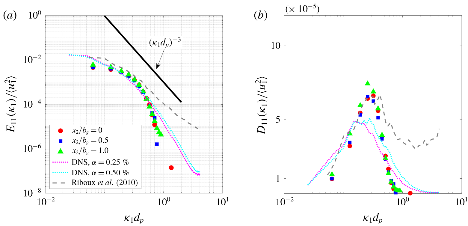
Figure 22. Comparison of (a) one-dimensional power spectra  $E_{11}(\unicode[STIX]{x1D705}_{1})$ of axial velocity fluctuations and (b) one-dimensional dissipation spectra in particle plume with earlier studies related to homogeneous bubble swarms (experiment, (Riboux et al. Reference Riboux, Risso and Legendre2010); DNS simulation, Lai et al. (Reference Lai, Fraga, Chan and Dodd2018)). The horizontal axis is normalized by the wavenumber corresponding to respective particle diameter ( $d_{p}$).
The one-dimensional dissipation spectra  $D_{11}(\unicode[STIX]{x1D705}_{1})=2\unicode[STIX]{x1D708}\unicode[STIX]{x1D705}^{2}E_{11}(\unicode[STIX]{x1D705}_{1})$ is shown in figure 22(b). Quite strikingly, the peaks of dissipation for our data and bubble plume/swarms reside at $\unicode[STIX]{x1D705}_{1}d_{p}\approx 0.2{-}0.4$. This indicates that in both bubble- and particle-laden turbulence, production and dissipation occur near the scale of particle size. This lack of scale separation was first postulated for homogeneous bubbly flows in Lance & Bataille (Reference Lance and Bataille1991) and is observed in direct numerical simulations reported in Lai et al. (Reference Lai, Fraga, Chan and Dodd2018).
4 Conclusions
We report an experimental study characterizing the turbulence inside a heavy particle plume descending under gravity within a salt–water solution. We measure the three components (i.e. 2D3C) of the interstitial fluid velocity and the spatial distribution of particles in the central plane of the plume using refractive-index-matched stereoscopic particle image velocimetry. Below we summarize our key findings primarily in the light of the results for a bubble plume (Lai & Socolofsky Reference Lai and Socolofsky2019).
The induced liquid flow inside the plume evolves with the mean flow characteristics of a bubble plume (Lai & Socolofsky Reference Lai and Socolofsky2019), that show Gaussian mean axial velocity ( $\langle U_{1}\rangle$) profile. The radial profiles of mean particle number density are also Gaussian with a half-width $b_{\unicode[STIX]{x1D719}}$ equals to $0.56b_{g}$, where $b_{g}$ is the Gaussian half-width of the mean streamwise velocity profile in the fluid.
The turbulence inside the plume is highly anisotropic with maximum streamwise turbulence intensity measuring up to 2.7 times that of the other two components, a result consistent with that observed in a bubble plume. The p.d.f. of the axial velocity fluctuation ( $u_{1}$) at the centreline of the plume is skewed so that the strongest events are in the direction opposite to mean flow. This behaviour is strikingly opposite to that observed previously for a bubble plume and a homogeneous swarm of bubbles. The turbulent kinetic energy and the in-plane shear-stress peak near ${\approx}0.75b_{g}$, locating the shear layer slightly outside the edge of the particle core ( $b_{\unicode[STIX]{x1D719}}$). Although these quantities for a bubble plume in Lai & Socolofsky (Reference Lai and Socolofsky2019) peaked at a similar location ( ${\approx}0.7b_{g}$), the location of the shear layer with respect to their bubble-core ( $b_{\unicode[STIX]{x1D719}}$) remains unknown.
Another distinction between the particle and the bubble plume is observed in the fluid-shear production term,  $P_{s}$, in the TKE budget. While the shear production in the bubble plume is negligible across the plume compared to the other terms, we observe a distinct peak in $P_{s}$ at the shear layer region of a particle plume, resembling a single-phase jet.
The other TKE terms including advection,  $A$, and the turbulent transport, $T$, in the two flows exhibit similar profiles. Further, we show that the turbulent transport, $T$, term follows similar qualitative profiles for both plumes and also an earlier reported variable-density single-phase jet (Charonko & Prestridge Reference Charonko and Prestridge2017), all of which differ from a typical single-phase jet. The difference in the relative magnitude in $T$ at the centreline between the two plumes is attributed to the difference in their third moment (skewness) of the axial velocity fluctuations.
Despite the above differences inside the core, both particle and bubble plumes show qualitatively that the TKE production by the particles,  $P_{b}$, approximately balances the mean dissipation rate, $\langle \unicode[STIX]{x1D716}\rangle$, away from the centreline. Further, the one-dimensional spectrum in the particle plume exhibits the $-3$ power law consistent with bubble plume and homogeneous swarms of bubbles. These two results support the notion that there is a lack of separation between the scales of production and dissipation in multiphase turbulent flows like ours.
Acknowledgements
This research was supported by the National Science Foundation (grant no. OCE-1334788) and by The Gulf of Mexico Research Initiative. The authors also thank M. Heath for his help in the design of the experimental set-up and data collection.
Declaration of interests
The authors report no conflict of interest.
Appendix A.
Table 6. Coefficients of double-Gaussian function in (A 1) used to fit various parameters measured in the experiment.
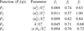
The three components of normal stresses, the turbulent kinetic energy ( $k$) and the mean dissipation rate $\langle \unicode[STIX]{x1D716}\rangle$ are fitted into a shape preserving double-Gaussian curve, given in (A 1) as follows:
 $$\begin{eqnarray}F_{i}(\unicode[STIX]{x1D702})=f_{1}\left[\text{exp}\left(-\left(\frac{\unicode[STIX]{x1D702}-f_{3}}{f_{2}}\right)^{2}\right)+\text{exp}\left(-\left(\frac{\unicode[STIX]{x1D702}+f_{3}}{f_{2}}\right)^{2}\right)\right].\end{eqnarray}$$
 All terms are expressed in similarity variable  $\unicode[STIX]{x1D702}=r/b_{g}$.
The in-plane shear-stress is fitted into a polynomial-Gaussian function in (A 2) as follows:
 $$\begin{eqnarray}S=\langle u_{z}u_{r}\rangle /U_{c}^{2}=(0.0124\unicode[STIX]{x1D702}+0.0286\unicode[STIX]{x1D702}^{3}-0.0113\unicode[STIX]{x1D702}^{5})\text{exp}(-1.47\unicode[STIX]{x1D702}^{2}).\end{eqnarray}$$
 The axial and radial transport of the turbulent kinetic energy ( $k$) are fitted into the polynomial-Gaussian functions in (A 3) and (A 4), respectively, as
 $$\begin{eqnarray}\displaystyle & T_{1}=\langle u_{z}k\rangle /U_{c}^{3}=(-0.0016-0.0252\unicode[STIX]{x1D702}^{2}-0.0181\unicode[STIX]{x1D702}^{4}+0.0746\unicode[STIX]{x1D702}^{6})\text{exp}(-2.62\unicode[STIX]{x1D702}^{2}),\qquad & \displaystyle\end{eqnarray}$$
 $$\begin{eqnarray}\displaystyle & T_{2}=\langle u_{r}k\rangle /U_{c}^{3}=(-0.0008\unicode[STIX]{x1D702}0.0048\unicode[STIX]{x1D702}^{3}-0.0139\unicode[STIX]{x1D702}^{5}-0.0049\unicode[STIX]{x1D702}^{7})\text{exp}(-1.76\unicode[STIX]{x1D702}^{2}).\qquad & \displaystyle\end{eqnarray}$$
Appendix B.
Expressions for the advection,  $A$, shear-production, $P_{s}$, and turbulent transport, $T$, terms in cylindrical coordinate system in the turbulent kinetic energy budget are summarized below. Each term is expressed in terms of the similarity variable $\unicode[STIX]{x1D702}=r/b_{g}$.
(i) Advection term
 $$\begin{eqnarray}A=-\left[\langle U_{z}\rangle \frac{\unicode[STIX]{x2202}k}{\unicode[STIX]{x2202}z}+\langle U_{r}\rangle \frac{\unicode[STIX]{x2202}k}{\unicode[STIX]{x2202}r}\right],\end{eqnarray}$$(B 1)$$\begin{eqnarray}A\times \frac{b_{g}}{U_{c}^{3}}=\left[\frac{2}{3}F_{4}(\unicode[STIX]{x1D702})+\unicode[STIX]{x1D702}\frac{\text{d}F_{4}(\unicode[STIX]{x1D702})}{\text{d}\unicode[STIX]{x1D702}}\right]\unicode[STIX]{x1D6FD}\text{e}^{-\unicode[STIX]{x1D702}^{2}}-\left[G(\unicode[STIX]{x1D702})\frac{\text{d}F_{4}(\unicode[STIX]{x1D702})}{\text{d}\unicode[STIX]{x1D702}}\right].\end{eqnarray}$$
(ii) Production term
$$\begin{eqnarray}P=-\left[\underbrace{\langle u_{z}^{2}\rangle \frac{\unicode[STIX]{x2202}\langle U_{z}\rangle }{\unicode[STIX]{x2202}z}}_{P_{1}}+\underbrace{\langle u_{r}^{2}\rangle \frac{\unicode[STIX]{x2202}\langle U_{r}\rangle }{\unicode[STIX]{x2202}r}}_{P_{2}}+\underbrace{\frac{\langle U_{r}\rangle \langle u_{\unicode[STIX]{x1D703}}^{2}\rangle }{r}}_{P_{3}}+\underbrace{\langle u_{z}u_{r}\rangle \left(\frac{\unicode[STIX]{x2202}\langle U_{z}\rangle }{\unicode[STIX]{x2202}r}+\frac{\unicode[STIX]{x2202}\langle U_{r}\rangle }{\unicode[STIX]{x2202}z}\right)}_{P_{4}}\right],\end{eqnarray}$$(B 2)$$\begin{eqnarray}\displaystyle & \displaystyle P_{1}\times \frac{b_{g}}{U_{c}^{3}}=\frac{\unicode[STIX]{x1D6FD}}{3}F_{1}(\unicode[STIX]{x1D702})\text{e}^{-\unicode[STIX]{x1D702}^{2}}(1-6\unicode[STIX]{x1D702}^{2}), & \displaystyle\end{eqnarray}$$(B 3)$$\begin{eqnarray}\displaystyle & \displaystyle P_{2}\times \frac{b_{g}}{U_{c}^{3}}=-F_{2}(\unicode[STIX]{x1D702})\frac{\text{d}G(\unicode[STIX]{x1D702})}{\text{d}\unicode[STIX]{x1D702}}, & \displaystyle\end{eqnarray}$$(B 4)$$\begin{eqnarray}\displaystyle & \displaystyle P_{3}\times \frac{b_{g}}{U_{c}^{3}}=-\frac{1}{\unicode[STIX]{x1D702}}F_{3}(\unicode[STIX]{x1D702})G(\unicode[STIX]{x1D702}), & \displaystyle\end{eqnarray}$$(B 5)$$\begin{eqnarray}\displaystyle & \displaystyle P_{4}\times \frac{b_{g}}{U_{c}^{3}}=S(\unicode[STIX]{x1D702})\left(2\unicode[STIX]{x1D702}\text{e}^{-\unicode[STIX]{x1D702}^{2}}+\frac{\unicode[STIX]{x1D6FD}}{3}G(\unicode[STIX]{x1D702})+\unicode[STIX]{x1D702}\unicode[STIX]{x1D6FD}\frac{\text{d}G(\unicode[STIX]{x1D702})}{\text{d}\unicode[STIX]{x1D702}}\right). & \displaystyle\end{eqnarray}$$(iii) Turbulent transport
$$\begin{eqnarray}T=-\left[\frac{\unicode[STIX]{x2202}\langle u_{z}k\rangle }{\unicode[STIX]{x2202}z}+\frac{1}{r}\frac{\unicode[STIX]{x2202}\langle u_{r}k\rangle }{\unicode[STIX]{x2202}r}\right],\end{eqnarray}$$(B 6)$$\begin{eqnarray}T\times \frac{b_{g}}{U_{c}^{3}}=\unicode[STIX]{x1D6FD}\left(T_{1}(\unicode[STIX]{x1D702})+\unicode[STIX]{x1D702}\frac{\text{d}T1}{\text{d}\unicode[STIX]{x1D702}}\right)-\left(\frac{T_{2}(\unicode[STIX]{x1D702})}{\unicode[STIX]{x1D702}}+\frac{\unicode[STIX]{x2202}T_{2}(\unicode[STIX]{x1D702})}{\unicode[STIX]{x2202}\unicode[STIX]{x1D702}}\right).\end{eqnarray}$$


 Open access