


1. Introduction
The relationship between the flow structure (such as the velocity and vorticity field) and forces acting on the body has attracted interest for a long time (Polhamus Reference Polhamus1966; Wang Reference Wang2005; Li, Dong & Zhao Reference Li, Dong and Zhao2018). Unsteady force approaches explaining this relationship are useful in understanding the physical mechanisms in natural flows, especially where vortical flow dominates, such as fish locomotion (Wu Reference Wu2011), flying seeds (Cummins et al. Reference Cummins, Seale, Macente, Certini, Mastropaolo, Viola and Nakayama2018), and insects’ and birds’ wings (Bomphrey et al. Reference Bomphrey, Nakata, Phillips and Walker2017; Usherwood et al. Reference Usherwood, Cheney, Song, Windsor, Stevenson, Dierksheide, Nila and Bomphrey2020), as well as in engineering problems such as dynamic stall (Li & Feng Reference Li and Feng2022), design and optimization of air vehicles (Alejandro et al. Reference Alejandro, Mustafa, Matej and Bas2018), cars (Liu et al. Reference Liu, Zhang, Zhang and Zhou2021), wind turbines (Dong, Viré & Li Reference Dong, Viré and Li2022), and so forth. Aside from being a theoretical point of interest, exploring the numerical connection between flow field and fluid forces has practical applications in experimental techniques such as particle image velocimetry (PIV) (Bird et al. Reference Bird, Ramesh, Ōtomo and Viola2022). Here, as well as the measurements being complicated by the inertia of the solid bodies, it may be difficult to obtain accurate flow information near solid surfaces compared to that in numerical simulations, limiting the use of pressure-based fluid force computations and hence necessitating the development of unsteady force methods.
A number of such approaches exist to extract aerodynamic and hydrodynamic forces from flow parameters, using velocity and/or its time or spatial derivative (Moreau Reference Moreau1952; Lin & Rockwell Reference Lin and Rockwell1996; Noca Reference Noca1996; Noca, Shiels & Jeon Reference Noca, Shiels and Jeon1997; Zhu, Bearman & Graham Reference Zhu, Bearman and Graham2002, Reference Zhu, Bearman and Graham2007). These approaches are usually derived based on the algebraic Bernoulli equation (Xia & Mohseni Reference Xia and Mohseni2013), the unsteady Blasius equation (Milne-Thomson Reference Milne-Thomson1960; Streitlien & Triantafyllou Reference Streitlien and Triantafyllou1995; Ford & Babinsky Reference Ford and Babinsky2013) and the moment-equation-based integral formulae (Howe Reference Howe1995; Saffman Reference Saffman1995). Except for these theoretical force approaches, there have been many experimental and computational studies verifying and utilizing the aforementioned methods, examples including experimental works such as those by Norberg (Reference Norberg2003), Birch & Dickinson (Reference Birch and Dickinson2003) and Shew, Poncet & Pinton (Reference Shew, Poncet and Pinton2006), and computational works from Ploumhans et al. (Reference Ploumhans, Winckelmans, Salmon, Leonard and Warren2002) and Hsieh et al. (Reference Hsieh, Kung, Chang and Chu2010). However, there has not been much in the way of theoretical updates on these works.
Recently, Li & Wu (Reference Li and Wu2018) proposed the vortex force map (VFM) method to extract force from the velocity and vorticity fields, making use of the integral force formula by Howe (Reference Howe1995). The VFM method was further explored and utilized to evaluate unsteady fluid dynamic forces in viscous flows from the vorticity field by Li et al. (Reference Li, Wang, Graham and Zhao2021). In this approach, forces acting on a body are expressed as a scalar product between the velocity, the vortex force vector and the local vortex strength. The VFMs, constructed in order to identify the force contribution effect of each vortex in the flow field, are dependent only on the body geometry and not on flow features. Moreover, the map provides a visual display of the force-producing and -reducing critical regions and directions. An extension to three-dimensional flows with application to a delta wing was later demonstrated by Li, Zhao & Graham (Reference Li, Zhao and Graham2020b), and the extension to the moment on an aerofoil was demonstrated by Li et al. (Reference Li, Wang, Graham and Zhao2020a). This was followed by the treatment of low Reynolds number flows in Li et al. (Reference Li, Wang, Graham and Zhao2021), extending the VFM method to more general cases for a wider range of Reynolds numbers (from  $O (10)$ to $O (1\times 10^6)$) by adding the viscous-pressure force and skin-friction force contributions to the total force. The formulation for vortex-pressure force maps was also updated so that vortices far away from the body have a vanishing effect on the force, making it possible to identify the force contribution effect of each given vortex based solely on the near-field flow. To facilitate its application in extracting forces from PIV-like flow velocity and vorticity data, the dependence of accuracy on the resolution of the mesh used to compute the forces, as well as the calculation/integration domain, were also investigated in that work. Note that here, a mesh is used to demonstrate the flow fields inferred from PIV data where the velocity/vorticity field data are pre-provided for the force calculation, while in other cases like the vortex panel method, a mesh is no longer needed.
So far, the methods described above all consider flows around a single body; it has been less clear how flows involving multiple bodies can be treated by these methods. Bai, Li & Wu (Reference Bai, Li and Wu2014) proposed the generalized Kutta–Joukowski force formula for two-dimensional inviscid flow involving multiple bound and free vortices, multiple aerofoils, and vortex generation (vorticity production) by using a specific momentum approach. Chang, Yang & Chu (Reference Chang, Yang and Chu2008) proposed a many-body force decomposition approach by employing auxiliary potential functions with applications to flow around an arrangement of multiple cylinders. However, Howe's original approach aimed at multi-body flows still needs further exploration since its application in aerofoil or wing aerodynamics is not complete. Moreover, the Chang et al. (Reference Chang, Yang and Chu2008) theory does not lend itself to a visual representation of the individual force contributions to each body from the vorticity distribution in the flow field. Therefore, in this work, the VFM method is extended to multi-body flows by deriving the vortex force formula for each individual body in a multi-body set-up. Similar to the previous work, we break down the contribution into three effects: the vortex-pressure force caused by free vorticity in the flow field, the viscous-pressure force, and the skin-friction force caused by vorticity on the body surface. For the first time, we aim to develop individual vortex-pressure force maps for each body in the presence of other bodies. To demonstrate its application, this method is used to study impulsively started flows around wing–flap configurations and validate the results against computational fluid dynamics (CFD) results. Subsequently, we will also use the method to study the force oscillation behaviour related to the vortex flow pattern.
In § 2, the derivation of the VFM approach for multi-body force decomposition is presented, with guidance on designing vortex-pressure force maps and applying the force approach in calculating total force. In § 3, vortex-pressure force map analysis for two-dimensional wing–flap configurations at different stages of deployment and at different angles of attack is demonstrated. Section 4 is dedicated to the application of the VFM approach to unsteady flows around the wing–flap configurations with different deflection angles of the flap, at different Reynolds numbers, and for different angles of attack. Theoretical results of force variation with time are validated against CFD. Concluding remarks are given in § 5.
2. Vortex force decomposition for multi-body flows
Consider viscous flows of constant density  $\rho$ and viscosity $\mu$ around a number $M$ of solid bodies. Each body has a volume $\varOmega _{mB}$ ( $m=1,2,\ldots,M$) bounded by closed surfaces $S_{mB}$ ( $m=1,2,\ldots,M$). (In the two-dimensional case, the bounding surface $S_{mB}$ reduces to a closed curve $l_{mB}$.) All bodies are assumed to be stationary relative to each other. The control volume $\varOmega$ is bounded by $S_{\infty }$ at infinity. In this section, we will derive the force $\boldsymbol {F}_{i}$ acting on the $i$th body, which can be decomposed into a normal component $F_{iN}$ and an axial component $F_{iA}$, or a lift component $L_{i}$ and a drag component $D_{i}$ in the body-fixed frame $( x,y,z)$ of the $i$th body. Here, the free-stream velocity is $V_{\infty }$ (incident at an angle $\alpha$ to the $i$th body axis), the velocity of the flow field is $\boldsymbol {U}$, the pressure is $P$, and the vorticity is $\boldsymbol {\omega }$. The problem set-up and the schematic of the flow and the force components are shown in figure 1. The flow is governed by the incompressible momentum equation in the Lamb–Gromyko form
 \begin{equation} \boldsymbol{\nabla} \left(P+\frac{1}{2}\,\rho U^{2}\right) +\rho \boldsymbol{\omega}\times \boldsymbol{U}={-}\rho\, \frac{\partial \boldsymbol{U}}{\partial t}-\mu\,\boldsymbol{\nabla} \times \boldsymbol{\omega}, \end{equation}
and the incompressible continuity equation
 \begin{equation} \boldsymbol{\nabla}\boldsymbol{\cdot} \boldsymbol{U}=0 . \end{equation}
Figure 1. (a) A set of rigid bodies  $\varOmega _{mB}$ ( $m=1,2,\ldots,M$), bounded by $S_{mB}$, in translational outer flows with a control volume $\varOmega$ bounded by $S_{\infty }$ at infinity. The force acting on the $i$th body may be either decomposed into a normal component ( $F_{iN}$) and an axial component ( $F_{iA}$), or a lift component ( $L_{i}$) and a drag component ( $D_{i}$). (b) A schematic display, depicted from a real flow, of a vortical flow field for a wing–flap configuration at an arbitrary angle of attack $\alpha$ ( $x$ is along the chord line, and $y$ is perpendicular to the chord line) and its various force components. Here, the total number of bodies is $M=2$, and $m=1$ denotes the main aerofoil, $m=2$ denotes the flap.
For each body  $i$, a set of hypothetical velocity potentials $\phi _{ik}$ is introduced here for the derivation of force acting on the $i$th body as a function of the vorticity field, similar to that suggested by Howe (Reference Howe1995) for a single-body case. Each $\phi _{ik}$ corresponds to the velocity potential for hypothetical potential fluid induced by the translational motion of $\varOmega _{iB}$ at unit speed in the $k$th direction (other bodies remain stationary for this purpose). According to the definition of the hypothetical potentials, they satisfy the Laplace equation in the entire field with boundary conditions
 \begin{equation}
\left.\begin{gathered} \nabla^{2}\phi _{i}=0, \\
\boldsymbol{\nabla} \boldsymbol{\phi}_{ik}\boldsymbol{\cdot}
\boldsymbol{n}_{iB}={-}\boldsymbol{k}
\boldsymbol{\cdot}\boldsymbol{n}_{iB}=n_{iB,k},
\quad \left( x,y,z\right)\rightarrow S_{iB}, \\
\boldsymbol{\nabla} \boldsymbol{\phi} _{ik}\boldsymbol{\cdot}
\boldsymbol{n}_{mB}=\boldsymbol{0}, \quad \left( x,y,z\right)
\rightarrow S_{mB}\cup S_{\infty }\left( m\neq
i\right). \end{gathered}\right\}.
\end{equation}
\begin{equation}
\left.\begin{gathered} \nabla^{2}\phi _{i}=0, \\
\boldsymbol{\nabla} \boldsymbol{\phi}_{ik}\boldsymbol{\cdot}
\boldsymbol{n}_{iB}={-}\boldsymbol{k}
\boldsymbol{\cdot}\boldsymbol{n}_{iB}=n_{iB,k},
\quad \left( x,y,z\right)\rightarrow S_{iB}, \\
\boldsymbol{\nabla} \boldsymbol{\phi} _{ik}\boldsymbol{\cdot}
\boldsymbol{n}_{mB}=\boldsymbol{0}, \quad \left( x,y,z\right)
\rightarrow S_{mB}\cup S_{\infty }\left( m\neq
i\right). \end{gathered}\right\}.
\end{equation} Here,  $\boldsymbol {n}_{iB}$ and $\boldsymbol {n}_{mB}$ are the normal vectors pointing inwards from each body surface, and $\boldsymbol {k}$ is the unit vector in the $k$th-direction.
2.1. General vortex force expression for the  $i$th body in three dimensions

In this subsection, we will derive the general vortex force expression for the multi-body assembly, a method that originated from Howe (Reference Howe1995) and Chang et al. (Reference Chang, Yang and Chu2008). According to the most commonly used force decomposition, the force acting on the  $i$th body is comprised of the pressure force and the skin-friction force,
 $$\begin{gather} \boldsymbol{F}_{i}=\boldsymbol{F}_{i}^{\left( pressure\right) }+ \boldsymbol{F}_{i}^{(friction) }, \end{gather}$$
 $$\begin{gather}\boldsymbol{F}_{i}^{(pressure) }=\iint_{S_{iB}}P \boldsymbol{n}_{iB}\,{\rm d} S, \end{gather}$$
 $$\begin{gather}\boldsymbol{F}_{i}^{(friction) }=\mu \iint_{S_{iB}} \boldsymbol{n}_{iB}\times \boldsymbol{\omega}\,{\rm d} S, \end{gather}$$
among which the pressure force can be transformed into a function of the vorticity field by using the Lamb–Gromyko equation (2.1) and the boundary condition (2.3) satisfied on the body surface.
Integrating the scalar product of  $\boldsymbol {\nabla } \phi _{ik}$ and (2.1) on the control volume (i.e. $\iiint _{\varOmega }\boldsymbol {\nabla } \phi _{ik}\boldsymbol{\cdot} \textrm {(\ref {eqn1})}\,\textrm {d}\varOmega$), with the help of the incompressible continuity equation (2.2) and the identities $\psi \,\boldsymbol {\nabla } \boldsymbol{\cdot} \boldsymbol {G}\equiv \boldsymbol {\nabla } \boldsymbol{\cdot} (\psi \boldsymbol {G}) -\boldsymbol {\nabla } \psi \boldsymbol{\cdot} \boldsymbol {G}$ and $\boldsymbol {\nabla } \boldsymbol{\cdot} (\boldsymbol {\nabla } \times \boldsymbol {G}) \equiv 0$ (where $\psi$ denotes an arbitrary scalar, and $\boldsymbol {G}$ is an arbitrary tensor), we have
 \begin{align} \iiint_{\varOmega}\boldsymbol{\nabla} \boldsymbol{\cdot} ( P\,\boldsymbol{\nabla} \phi _{ik})\,{\rm d}\varOmega &={-}\rho \iiint_{\varOmega}\boldsymbol{\nabla} \boldsymbol{\cdot} \left(\phi _{ik}\, \frac{\partial \boldsymbol{U}}{\partial t}\right) {\rm d}\varOmega -\rho \iiint_{\varOmega }\boldsymbol{\nabla} \phi _{ik}\boldsymbol{\cdot} \left( \boldsymbol{\omega }\times \boldsymbol{U}\right) {\rm d}\varOmega \nonumber\\ &\quad -\mu \iiint_{\varOmega}\boldsymbol{\nabla} \boldsymbol{\cdot} \left(\phi _{ik}\,\boldsymbol{\nabla} \times\boldsymbol{\omega }\right) {\rm d}\varOmega. \end{align}
Applying Green's theorem to transform the volume integral in the above equation into the surface integral, and with the application of the identity  $\phi _{ik}\,\boldsymbol {\nabla } \times \boldsymbol {\omega }=\boldsymbol {\nabla } \times ( \phi _{ik} \boldsymbol {\omega }) +\boldsymbol {\omega }$ $\times \boldsymbol {\nabla } \phi _{ik}$ and $\iint _{S}\boldsymbol {\nabla } \times \boldsymbol {G}\boldsymbol{\cdot} \boldsymbol {n}\,\textrm {d} S=0$ on any enclosed surfaces, we have
 \begin{align}
&{-}\iint_{S_{1B}+S_{2B}+\cdots+S_{MB}+S_{\infty}}\boldsymbol{P}\,\boldsymbol{\nabla}
\boldsymbol{\phi}_{ik}\boldsymbol{\cdot}\boldsymbol{n}_{mB}\,{\rm d} S \nonumber\\ &\quad={-}\rho
\iint_{S_{1B}+S_{2B}+\cdots+S_{MB}+S_{\infty}}\phi
_{ik}\, \frac{\partial \boldsymbol{U}}{\partial t}\boldsymbol{\cdot}
\boldsymbol{n}\,{\rm d} S -\rho
\iiint_{\varOmega}\boldsymbol{\nabla} \phi _{ik}\boldsymbol{\cdot}
\left( \boldsymbol{ \omega }\times \boldsymbol{U}\right)
{\rm d}\varOmega \nonumber\\ &\qquad-\mu
\iint_{S_{1B}+S_{2B}+\cdots+S_{MB}+S_{\infty}}\boldsymbol{\omega}\times
\boldsymbol{\nabla} \phi _{ik}\boldsymbol{\cdot} \boldsymbol{n}\,{\rm
d} S. \end{align}
\begin{align}
&{-}\iint_{S_{1B}+S_{2B}+\cdots+S_{MB}+S_{\infty}}\boldsymbol{P}\,\boldsymbol{\nabla}
\boldsymbol{\phi}_{ik}\boldsymbol{\cdot}\boldsymbol{n}_{mB}\,{\rm d} S \nonumber\\ &\quad={-}\rho
\iint_{S_{1B}+S_{2B}+\cdots+S_{MB}+S_{\infty}}\phi
_{ik}\, \frac{\partial \boldsymbol{U}}{\partial t}\boldsymbol{\cdot}
\boldsymbol{n}\,{\rm d} S -\rho
\iiint_{\varOmega}\boldsymbol{\nabla} \phi _{ik}\boldsymbol{\cdot}
\left( \boldsymbol{ \omega }\times \boldsymbol{U}\right)
{\rm d}\varOmega \nonumber\\ &\qquad-\mu
\iint_{S_{1B}+S_{2B}+\cdots+S_{MB}+S_{\infty}}\boldsymbol{\omega}\times
\boldsymbol{\nabla} \phi _{ik}\boldsymbol{\cdot} \boldsymbol{n}\,{\rm
d} S. \end{align}
Substituting (2.3) into the left-hand side of (2.6), we have
 \begin{equation} -\iint_{S_{1B}+S_{2B}+\cdots+S_{MB}+S_{\infty}}\boldsymbol{P}\,\boldsymbol{\nabla} \boldsymbol{\phi}_{ik}\boldsymbol{\cdot} \boldsymbol{n}_{mB}\,{\rm d} S=\iint_{S_{iB}}Pn_{iB,k}\,{\rm d} S. \end{equation}
As the flow at infinity is undisturbed and irrotational, we have
 $$\begin{gather} \rho \iint_{S_{\infty }}\phi _{ik}\,\frac{\partial \boldsymbol{U}}{ \partial t}\boldsymbol{\cdot} \boldsymbol{n}\,{\rm d} S=0, \end{gather}$$
 $$\begin{gather}\mu \iint_{S_{\infty }}\boldsymbol{\omega }\times \boldsymbol{\nabla} \phi_{ik}\boldsymbol{\cdot} \boldsymbol{n}\,{\rm d} S=0. \end{gather}$$
 Projecting the force equation (2.4c) into the  $k$th direction and substituting (2.6)–(2.8) into it, we arrive at the formulas (2.9) below, which express the $k$th component of the force of the $i$th body in the form of a summation of four components, namely the added mass force $F_{ik}^{(add)}$, the vortex-pressure force $F_{ik}^{(vor\textrm {-}p)}$, the viscous-pressure force $F_{ik}^{(vis\textrm {-}p)}$ and the skin-friction force $F_{ik}^{(friction)}$, and the first three make up the pressure force $F_{ik}^{(pressure)}$:
 $$\begin{gather} F_{{ik}}=\underset{F_{ik}^{(pressure)}}{\underbrace{F_{ik}^{(add)}+ F_{ik}^{(vor\text{-}p)}+F_{ik}^{(vis\text{-}p)}}}+F_{ik}^{(friction)}, \end{gather}$$
 $$\begin{gather}F_{ik}^{(add)}={-}\rho \sum_{i=1,2,\ldots,M} \iint_{S_{iB}}\phi _{ik}\, \frac{\partial \boldsymbol{U}}{\partial t}\boldsymbol{\cdot} \boldsymbol{n}\,{\rm d} S, \end{gather}$$
 $$\begin{gather}F_{ik}^{(vor\text{-}p)}={-}\rho \iiint_{\varOmega}\boldsymbol{\nabla} \phi_{ik}\boldsymbol{\cdot}\left(\boldsymbol{\omega }\times \boldsymbol{U}\right) {\rm d}\varOmega, \end{gather}$$
 $$\begin{gather}F_{ik}^{(vis\text{-}p)}={-}\mu \sum_{i=1,2,\ldots,M} \iint_{S_{iB}}\boldsymbol{ \omega }\times\boldsymbol{\nabla} \phi _{ik}\boldsymbol{\cdot} \boldsymbol{n}_{iB}\,{\rm d} S, \end{gather}$$
 $$\begin{gather}F_{ik}^{(friction)}=\mu \iint_{S_{iB}}\boldsymbol{n}_{B}\times \boldsymbol{\omega }\boldsymbol{\cdot} \boldsymbol{k}\,{\rm d} S. \end{gather}$$
 Some discussions on the force formula follow. (i) It is fully applicable to unsteady flows. For the first term (the added mass force)  $F_{ik}^{(add)}$, time is included explicitly by $\partial \boldsymbol {U}/\partial t$, while for the remaining terms, time is included implicitly by the time-dependent flow field data $\boldsymbol {\omega }$ and $\boldsymbol {U}$. (ii) The added mass force $F_{ik}^{(add)}$, proportional to $\partial \boldsymbol {U}/\partial t$ on the body surface, is caused by acceleration, pitching, heaving and deformation of the body. In the example case of the starting flow problem considered in this paper, $F_{ik}^{(add)}=0$. (iii) As will be shown in § 4, the vortex-pressure force $F_{ik}^{(vor\textrm {-}p)}$ is the dominant force. According to the definition of hypothetical potential (2.3), $\boldsymbol {\nabla } \phi _{ik}=0$ at infinity, which ensures that the above formula is consistent with the fact that only near-body vortices are more likely to cause pressure variation, while vortices far away from the body have negligible effects on the force. (iv) The viscous-pressure force $F_{ik}^{(vis\textrm {-}p)}$ and the skin-friction force $F_{ik}^{(friction)}$ contain the integration of vorticity $\boldsymbol {\omega }$ on the body surface. In practice, we interpolate the vorticity in the boundary layer to the body surface as an approximation. (v) The cross-terms in the added mass force $F_{ik}^{(add)}$ and in the viscous-pressure force $F_{ik}^{(vis\textrm {-}p)}$ contain explicitly the contributions of forces from other bodies. There are no explicit cross-interactions in the vortex-pressure force $F_{ik}^{(vor\textrm {-}p)}$; however, as we will see later, such interactions are included implicitly in $\phi _{ik}$.
2.2. General vortex force expression for the $i$th body in two dimensions

In two-dimensional flow, we have  $\boldsymbol {\nabla } =({\partial }/{\partial x},{\partial }/{\partial y},0)$, $\boldsymbol {\omega }=(0,0,\omega _{z})$ and $\boldsymbol {U}=( u,v,0)$. The force expressions (2.9) can now be simplified into
 $$\begin{gather} F_{{ik}}=\underset{F_{ik}^{(pressure)}}{\underbrace{F_{ik}^{(add)}+ F_{ik}^{(vor\text{-}p)}+F_{ik}^{(vis\text{-}p)}}}+F_{ik}^{(friction)}, \end{gather}$$
 $$\begin{gather}F_{ik}^{(add)}={-}\rho \sum_{i=1,2,\ldots,M} \iint_{l_{iB}}\phi _{ik}\, \frac{\partial \boldsymbol{U}}{\partial t}\boldsymbol{\cdot} \boldsymbol{n}\,{\rm d} l, \end{gather}$$
 $$\begin{gather}F_{ik}^{(vor\text{-}p)}=\rho \iint_{\varOmega}\boldsymbol{\varLambda}_{ik}\boldsymbol{\cdot} \boldsymbol{U}\omega_{z}\,{\rm d}\varOmega, \end{gather}$$
 $$\begin{gather}F_{ik}^{(vis\text{-}p)}=\mu \sum_{i=1,2,\ldots,M} \oint_{l_{iB}}\omega _{z}\,{\rm d}\phi_{ik}, \end{gather}$$
 $$\begin{gather}F_{i}^{(friction)}=\mu \oint_{l_{iB}}\omega _{z}\boldsymbol{k}\boldsymbol{\cdot} \boldsymbol{{\rm d} l}, \end{gather}$$
where  $\boldsymbol {U}=(u,v)$ is the vortex velocity in the $i$th body fixed frame. The integral in the vortex-pressure force term is defined within the whole fluid region $\varOmega$, and the viscous-pressure and skin-friction terms are defined along the body surface $l_{mB}$ ( $m=1,2,\ldots,M$). The vortex-pressure force factor is expressed as
 \begin{equation} \boldsymbol{\varLambda }_{ik}=\left( \frac{\partial \phi _{ik}}{\partial y}, -\frac{\partial \phi _{ik}}{\partial x}\right), \end{equation}
where  $\phi _{ik}$ is defined in (2.3).
2.3. Vortex lift and drag expression for the $i$th body in two dimensions

We now derive the forms of lift and drag forces from the general force expression. In extending the discussion of the vortex force method to multiple bodies in the preceding subsections, it might appear from the expression that the fluid forces on a single body can be understood as a superposition of the contributions from each individual body, occurring in the added mass and the viscous-pressure terms. However, we would now like to demonstrate that there are interactions implicit in the expression for the inertial, viscous and vortex force contributions that are beyond a superposition of its stand-alone components, but are present in the hypothetical potential  $\phi$. Consider, in the $i$th body fixed frame, that the free-stream velocity is $\boldsymbol {V_{\infty }}$ with incident angle $\alpha$. The lift expression for the $i$th body can be given by choosing the direction $\boldsymbol {k}=\boldsymbol {k}_{L}=( -\sin \alpha,\cos \alpha )$ in expressions (2.10):
 $$\begin{gather} L_{i}=\underset{L_{i}^{(pressure)}}{\underbrace{L_{i}^{(add)}+ L_{i}^{(vor\text{-}p)}+L_{i}^{(vis\text{-}p)}}}+L_{i}^{(friction)}, \end{gather}$$
 $$\begin{gather}L_{i}^{(add)}={-}\rho \sum_{i=1,2,\ldots,M} \iint_{l_{iB}}\phi_{iL}\, \frac{\partial \boldsymbol{U}}{\partial t}\boldsymbol{\cdot} \boldsymbol{n}\,{\rm d} l, \end{gather}$$
 $$\begin{gather}L_{i}^{(vor\text{-}p)}=\rho \iint_{\varOmega}\boldsymbol{\varLambda}_{iL}\boldsymbol{\cdot} \boldsymbol{U}\omega_{z}\,{\rm d}\varOmega, \end{gather}$$
 $$\begin{gather}L_{i}^{(vis\text{-}p)}=\mu \sum_{i=1,2,\ldots,M} \oint_{l_{iB}}\omega_{z}\,{\rm d}\phi_{iL}, \end{gather}$$
 $$\begin{gather}L_{i}^{(friction)}=\mu \oint_{l_{iB}}\omega_{z}\boldsymbol{k}_{L}\boldsymbol{\cdot} \boldsymbol{{\rm d} l}. \end{gather}$$
 Similarly, the drag expression for the  $i$th body can be given by choosing the direction $\boldsymbol {k}=\boldsymbol {k}_{D}=(\cos \alpha,\sin \alpha )$ in expressions (2.10):
 $$\begin{gather} D_{i}= \underset{D_{i}^{(pressure)}}{\underbrace{ D_{i}^{(add)}+D_{i}^{(vor\text{-}p)}+ D_{i}^{(vis\text{-}p)}}}+D_{i}^{(friction)}, \end{gather}$$
 $$\begin{gather}D_{i}^{(add)}={-}\rho \sum_{i=1,2,\ldots,M} \iint_{l_{iB}}\phi _{iD} \frac{\partial \boldsymbol{U}}{\partial t}\boldsymbol{\cdot} \boldsymbol{n}\,{\rm d} l, \end{gather}$$
 $$\begin{gather}D_{i}^{(vor\text{-}p)}=\rho \iint_{\varOmega}\boldsymbol{\varLambda}_{iD}\boldsymbol{\cdot} \boldsymbol{U}\omega_{z}\,{\rm d}\varOmega, \end{gather}$$
 $$\begin{gather}D_{i}^{(vis\text{-}p)}=\mu \sum_{i=1,2,\ldots,M} \oint_{l_{iB}}\omega_{z}\,{\rm d}\phi_{iD}, \end{gather}$$
 $$\begin{gather}D_{i}^{(friction)}=\mu \oint_{l_{iB}}\omega _{z}\boldsymbol{k}_{D} \boldsymbol{\cdot} \boldsymbol{{\rm d} l}. \end{gather}$$
Here, the vortex-pressure force vector for lift is
 \begin{equation} \boldsymbol{\varLambda}_{iL}=\left(\frac{\partial \phi _{iL}}{\partial y},- \frac{\partial \phi _{iL}}{\partial x}\right), \end{equation}
and for drag is
 \begin{equation} \boldsymbol{\varLambda }_{iD}=\left(\frac{\partial \phi _{iD}}{\partial y},- \frac{\partial \phi _{iD}}{\partial x}\right). \end{equation}
The hypothetical potentials  $\phi _{iL}$ and $\phi _{iD}$ are induced by the translational movement of the $i$th body in the $\boldsymbol {k}_{L}=( -\sin \alpha,\cos \alpha )$ and $\boldsymbol {k}_{D}=( \cos \alpha,\sin \alpha )$ directions with unit velocity, respectively, i.e.
 \begin{align}& \left.\begin{gathered} \frac{\partial ^{2}\phi _{iL}}{\partial x^{2}}+\frac{\partial ^{2}\phi _{iL} }{\partial y^{2}}=0, \\ \frac{\partial \phi _{iL}}{\partial n}=\boldsymbol{n}\boldsymbol{\cdot} \left(-\sin \alpha,\cos \alpha \right),\quad (x,y)\rightarrow l_{iB}, \\ \frac{\partial \phi _{iL}}{\partial x}=\frac{\partial \phi _{iL}}{\partial y} =0,\quad (x,y) \rightarrow l_{mB}\left( m\neq i\right)\cup S_{\infty}, \end{gathered}\right\} \end{align}
 \begin{align}& \left.\begin{gathered} \frac{\partial^{2}\phi _{iD}}{\partial x^{2}}+\frac{\partial ^{2}\phi_{iD}}{\partial y^{2}}=0, \\ \frac{\partial \phi _{iD}}{\partial n}=\boldsymbol{n}\boldsymbol{\cdot} \left(\cos \alpha,\sin \alpha \right), \quad (x,y)\rightarrow l_{iB}, \\ \frac{\partial \phi _{iD}}{\partial x}=\frac{\partial \phi _{iD}}{\partial y} =0,\quad (x,y) \rightarrow l_{mB}\left( m\neq i\right)\cup S_{\infty }. \end{gathered}\right\} \end{align}
 Thus, to obtain the vortex force factors  $\boldsymbol {\varLambda }_{iL}$ and $\boldsymbol {\varLambda }_{iD}$, one simply needs to solve the Laplace models (2.16) and (2.17). It should again be stressed that in order to identify the vortex force contributions to individual bodies, the extension of hypothetical potentials to multiple bodies should be treated as the potential that would have been obtained by giving the body being considered a unit hypothetical velocity in the direction considered, while keeping other bodies fixed. We have thus demonstrated that while the concept of the VFM for an individual body still exists in a multi-body set-up, the mere presence of other bodies in the flow field will serve to modify the VFMs by effectively creating additional boundary conditions in the solution for the hypothetical potential. Therefore the multi-body extension of the vortex map method should not be understood or treated as a simple superposition of the contributions from individual bodies.
2.4. Method to plot vortex-pressure force maps and calculate total force
We now put the focus of our analysis on the vortex-pressure term in the force formulas (2.12) and (2.13) as studies have shown that the forces are dominated by the vortex forces for massively separated flow problems (Ansari, Żbikowski & Knowles Reference Ansari, Żbikowski and Knowles2006; Xia & Mohseni Reference Xia and Mohseni2013). Expressions (2.12) and (2.13) give the force as the function of the vorticity field, in which the free vorticity in the flow field contributes to the pressure force, and the vorticity on the body surface contributes to both pressure force and skin-friction force. As will be discussed later, the dominant force component is vortex-pressure force, in the form of the integration of a scalar product between the vortex-pressure force vectors defined in (2.14) and (2.15), and the local velocity. The vortex-pressure force vectors are functions of position but independent of the flow field (including Reynolds number), and are dependent only on body shape and angle of attack. Thus the vortex-pressure force vectors can be pre-computed without knowing the flow field by solving (2.16) and (2.17) numerically. More details will be given in the next section.
On the one hand, these vectors can be used to build the vortex-pressure force maps that can help to analyse force oscillating behaviour in relation to the vortex flow pattern and identify the critical regions and directions for positive and negative force production by a given vortex.
On the other hand, the vectors can be used together with force formulas (2.12) and (2.13) to obtain total forces if the properties of vortices (velocity and circulation) in the flow field and on the body surface are obtained through analytical, numerical or experimental methods.
2.4.1. Vortex-pressure force map analysis
Vortex force maps in the two-dimensional plane  $(x,y)$ for the $i$th body are designed based on the precomputed vortex-pressure force vectors $\boldsymbol {\varLambda }_{iL}$ for lift force and $\boldsymbol {\varLambda }_{iD}$ for drag given by (2.14) and (2.15). Each map contains force lines that are locally parallel to the vortex force vectors, which can be obtained through a streamline procedure, with the velocity replaced by the vortex force factors. It also contains contours of $\vert \boldsymbol {\varLambda }_{iL} \vert$ or $\vert \boldsymbol {\varLambda }_{iD} \vert$. The VFM is defined in such a way that the force contribution of any individual vortex can be easily identified according to its circulation (sign and magnitude), position, and direction (the angle between the vortex force line and streamline at the point of the vortex). Thus lift-increasing or drag-reducing directions and critical regions of a given vortex for each body can be defined in a similar way as in Li & Wu (Reference Li and Wu2018).
2.4.2. Calculation of total force
With vortex force vectors pre-computed for the  $i$th body, once the velocity field $\boldsymbol {U}$ and vorticity field $\omega _{z}$ can be computed or measured, total forces can then be obtained directly from the vortex force formulas. This can be done as follows.
Given the geometry and position of  $M$ bodies, the lift and drag force vectors of the $i$th body at an angle of attack $\alpha$ can be given by finding the solution of hypothetical potentials $\phi _{iL}$ and $\phi _{iD}$ for the Laplace equations (2.16) and (2.17). The hypothetical potentials $\phi _{iL}$ and $\phi _{iD}$ are then substituted into expressions (2.14) and (2.15) to give the vortex force vectors $\boldsymbol {\varLambda }_{iL}$ and $\boldsymbol {\varLambda }_{iD}$. It is clear that for multi-body set-ups with relative motion, the hypothetical potential will need to be updated at each time step. However, in reality, the variation of the hypothetical potential with relative position is smooth as long as there is no contact between the bodies. It is easy to interpolate between different pre-computed relative positions to improve computational efficiency. In addition, the maps can be computed using a potential-type method at a very low computational cost. (i) For the vortex-pressure force, substitute $\boldsymbol {\varLambda }_{iL}$ and $\boldsymbol {\varLambda }_{iD}$ into the first terms of (2.12) and (2.13) to calculate vortex-pressure lift $L_{i}^{(vor\textrm {-}p)}$ and drag $D_{i}^{(vor\textrm {-}p)}$. (ii) For the viscous-pressure force, substitute $\phi _{iL}$ and $\phi _{iD}$ into the second terms of (2.12) and (2.13) to obtain the viscous-pressure lift $L_{i}^{(vis\textrm {-}p)}$ and drag $D_{i}^{(vis\textrm {-}p)}$. (iii) For the skin-friction force, we use the third terms in (2.12) and (2.13) to compute skin-friction lift $L_{i}^{(friction)}$ and drag $D_{i}^{(friction)}$.
These reduce to the case in Li et al. (Reference Li, Wang, Graham and Zhao2021) when there is only a single body.
3. Vortex-pressure force map analysis for wing–flap configurations
In this section, three slotted wing–flap configurations with deflection angles of the flap  $-20^{\circ }$, $0^{\circ }$ and $20^{\circ }$ are used to demonstrate the construction of the vortex-pressure force maps for a specific body among a series of bodies. We choose the NACA 64(3)-618 aerofoil as the base wing, and the slotted trailing edge flap takes up 15 % of the total chord. The vortex-pressure force maps can be used to identify the force contribution effect of each given vortex to each body according to its position, strength and local velocity. Here, we consider only lift and drag force maps, which depend on the geometry as well as the angle of attack.
For a wing–flap model, with geometry – the main aerofoil denoted as  $\varOmega _{1B}$, the flap denoted as $\varOmega _{2B}$, and the deflection angle denoted as $\delta$ – and angle of attack $\alpha$ given, the Laplace equations (2.16) and (2.17) are solved by using the vortex panel method as suggested by Katz & Plotkin (Reference Katz and Plotkin2001) in solving the steady-state potential flow. The method solves the Laplace equation via a superposition of singularity elements on the body surface and enforcing non-penetration boundary condition on the surface and zero total circulation, which has been validated against that solved by the commercial code CFX. In this solver, the solution for the hypothetical potential is the non-circulatory one among the infinite number of possibilities in two-dimensional flow. The vortex-pressure force vectors for lift ( $\boldsymbol {\varLambda }_{iL}$, $i=1,2$) and for drag ( $\boldsymbol {\varLambda }_{iD}$, $i=1,2$) are then computed by (2.14) and (2.15). With the vortex force factors pre-computed, the vortex-pressure force maps are then generated following the steps in § 2.4.
Figures 2–5 show the vortex-pressure force maps for wing–flap configurations. In these maps, the vortex force lines are represented as solid arrows that are parallel to the local vortex force vectors ( $\boldsymbol {\varLambda }_{iL}$ or $\boldsymbol {\varLambda }_{iD}$, $i=1,2$). The contour lines for the norm of vortex force vectors ( $\vert \boldsymbol {\varLambda }_{iL} \vert$ or $\vert \boldsymbol {\varLambda }_{iD} \vert$, $i=1,2$) are also presented. According to the vortex-pressure force maps, a counter-clockwise rotating vortex (e.g. a trailing edge vortex (TEV) rolled up on the trailing edge) contributes positive force (lift or drag) if it moves so as to have a component of motion in the direction of the vortex force lines, while a clockwise rotating vortex (e.g. a leading edge vortex (LEV) formed on the leading edge) contributes positive force (lift or drag) if it moves so as to have a component of motion opposed to the vortex force lines, and vice versa.
3.1. Influence of deflection angle of the flap on vortex-pressure force maps
Figure 2 shows the vortex-pressure force maps for both lift and drag of the main aerofoil ( $\varOmega _{1B}$) in the wing–flap configurations with different deflection angles of flap: $\delta =-20^{\circ }$, $0^{\circ }$ and $20^{\circ }$. We can see that the norms of the vortex force vectors $\vert \boldsymbol {\varLambda }_{1L} \vert$ and $\vert \boldsymbol {\varLambda }_{1D} \vert$ for the main aerofoil decrease with the distance from the wing–flap configuration, and the peak values are located in the leading edge area of the main aerofoil, the connecting area of two bodies, and the trailing edge area of the flap. The vortex force lines near the flap rotate accordingly with increasing the deflection angle of the flap; this can be seen more clearly by following the vortex force line projecting from the trailing edge of the flap. This observation should be put in the context that the method does not use information relating to actual flow fields and is unaware of separation points.
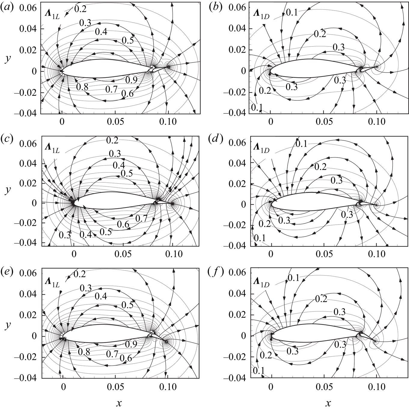
Figure 2. Vortex-pressure force maps for lift and drag of the main aerofoil at  $ \alpha =20^{\circ }$ with different flap angles: (a,c,e) lift with flap angles $ \delta =-20^{\circ }$, $0^{\circ }$ and $20^{\circ }$, respectively; (b,d,e) drag with the same flap angles. The lines with arrows are vortex-pressure force lines locally parallel to the vectors $ \boldsymbol {\varLambda }_{1L}$ and $ \boldsymbol {\varLambda }_{1D}$, and the lines without arrows are contours of the magnitudes of $ \boldsymbol {\varLambda }_{1L}$ and $ \boldsymbol {\varLambda }_{1D}$.
Figure 3 shows the vortex-pressure force maps for the flap ( $\varOmega _{2B}$) in the same wing–flap configurations. We can see that the norms of the vortex force vectors $\vert \boldsymbol {\varLambda }_{2L} \vert$ and $\vert \boldsymbol {\varLambda }_{2D} \vert$ for the flap decrease with the distance from the flap, and the peak values are located in the connecting area of two bodies and the trailing edge area of the flap. Again, the vortex force lines rotate with the deflection angle of the flap, which can be seen by following the line emanating from the trailing edge itself.

Figure 3. Vortex-pressure force maps for the lift and drag on the flap in the wing–flap configurations for  $ \alpha =20^{\circ }$ with different flap angles: (a,c,e) lift with flap angles $ \delta = -20^{\circ }$, $0^{\circ }$ and $20^{\circ }$, respectively; (b,d,e) drag with the same flap angles. The lines with arrows are vortex-pressure force lines locally parallel to the vectors $ \boldsymbol {\varLambda }_{2L}$ and $ \boldsymbol {\varLambda }_{2D}$, and the lines without arrows are contours of the magnitudes of $ \boldsymbol {\varLambda }_{2L}$ and $ \boldsymbol {\varLambda }_{2D}$.
3.2. Influence of angle of attack on vortex-pressure force maps
As in the VFM method proposed by Li & Wu (Reference Li and Wu2018), the multi-body VFM method in this work has the capability for flow problems at arbitrarily high angles where large separations are generated. To demonstrate this, three typical large angles of attack, i.e.  $\alpha =20^{\circ }$, $45^{\circ }$ and $60^{\circ }$, are chosen here. Figures 4 and 5 show the vortex-pressure force maps for both the lift and drag of the main aerofoil as well as the flap in a $\delta =0^{\circ }$ wing–flap configuration at $\alpha =45^{\circ }$ and $60^{\circ }$, respectively. Compared with those maps at $\alpha =20^{\circ }$ in figures 2(c,d) and 3(c,d), we can see that the vortex-pressure force maps for different angles of attack look similar. We can also see from these maps that the larger the angle of attack, the smaller the vortex lift factors, and the larger the vortex drag factors in corresponding positions. Note that in the present vortex-pressure force maps, the fact that vorticity far away from the body has a negligible effect on force is satisfied automatically.

Figure 4. Vortex-pressure force maps for lift and drag of the wing–flap configuration at  $ \alpha =45^{\circ }$ with zero deflection angle of flap: (a) lift of the main aerofoil; (b) drag of the main aerofoil; (c) lift of the flap; (d) drag of the flap. The lines with arrows are vortex-pressure force lines locally parallel to the vectors $ \boldsymbol {\varLambda }_{iL}$ and $ \boldsymbol {\varLambda }_{iD}$, and the lines without arrows are contours of the magnitudes of $ \boldsymbol {\varLambda }_{iL}$ and $ \boldsymbol {\varLambda }_{iD}$, where $i=1,2$, respectively.
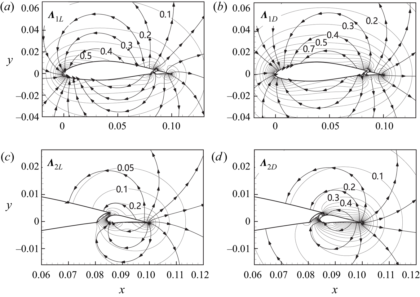
Figure 5. Vortex-pressure force maps for lift and drag of the wing–flap configuration at  $ \alpha =60^{\circ }$ with zero deflection angle of flap: (a) lift of the main aerofoil; (b) drag of the main aerofoil; (c) lift of the flap; (d) drag of the flap. The lines with arrows are vortex-pressure force lines locally parallel to the vectors $ \boldsymbol {\varLambda }_{iL}$ and $ \boldsymbol {\varLambda }_{iD}$, and the lines without arrows are contours of the magnitudes of $ \boldsymbol {\varLambda }_{iL}$ and $ \boldsymbol {\varLambda }_{iD}$, where $i=1,2$, respectively.
4. Vortex lift and drag for viscous flows around impulsively started wing–flap configurations
In this section, the VFM method is applied to an impulsively started wing–flap flow. Here, the total force will be given by (2.12) and (2.13), with the velocity and vorticity fields provided by CFD. The theoretical lift and drag results will be compared with those obtained from integrating the body surface pressure and skin-friction given by CFD code. Here, all the flow field is assumed to be laminar. The contribution of different force components, either from free vorticity in the flow field or from the vorticity on the body surface, will be discussed. The force oscillation on the main aerofoil as well as on the flap in relation to the evolution of the vortex structure in the flow field will be studied.
4.1. Force approach and CFD method
As discussed in § 2.4, the vortex force approach (2.12) and (2.13) can be used to calculate the total force acting on the body, with the vortex force factors pre-computed by analytical or numerical methods, and the velocity and vorticity fields given by conventional methods, including a vortex panel method, CFD simulation or experimental measurement. The accuracy of the single-body VFM method on truncated domains and under coarse sampling of typical PIV measurement size has been studied in previous work by Li & Wu (Reference Li and Wu2018), where the potential of the VFM method on experimental measurement has been demonstrated. However, the potential of the multi-body VFM method on experimental measurement and its sensitivity to experimental uncertainty remain for future work.
The results of pressure lift  $L_{i}^{(pressure)}$ and drag $D_{i}^{(pressure)}$ will be compared to the pressure lift and drag obtained by the integration of the body surface pressure in the CFD code, while the results of skin-friction force $L_{i}^{(friction)}$ and $D_{i}^{(friction)}$ will be compared to the skin-friction lift and drag obtained from the CFD code. Note that for the starting flow problem considered here, the added mass force $L_{i}^{(add)}$ and drag $D_{i}^{(add)}$ in (2.12) and (2.13) are infinite at the initial moment, and are $0$ at any moment after the starting procedure. Here, the force results will be represented in the form of non-dimensional coefficients. The lift and drag coefficients are defined as
 \begin{equation} C_{L}=\frac{L}{\tfrac{1}{2}\rho V_{\infty }^{2}c_{A}},\quad C_{D}=\frac{D}{\tfrac{1}{ 2}\rho V_{\infty }^{2}c_{A}}, \end{equation}
where  $c_{A}$ is the total chord length of the wing–flap configuration. The Reynolds number in this paper is defined based on the total chord length: ${Re}=\rho V_{\infty }c_{A}/\mu$. The time-dependent forces will be displayed as functions of the non-dimensional time $\tau =tV_{\infty }/c_{A}$.
In CFD, the Navier–Stokes equations for unsteady laminar flow are solved numerically using the same method as used by Li & Wu (Reference Li and Wu2018). Note that the purpose of this work is to study the capability and accuracy of the proposed multi-body VFM approach rather than an accurate simulation of separating flows, thus a laminar flow solution is used here. We have used the commercial code Fluent with a second-order upwind SIMPLE (semi-implicit method for pressure-linked equations) pressure–velocity coupling method. The computational domain is  $30\times c_{A}$ in the horizontal direction, and $20\times c_{A}$ in the vertical direction. Different mesh sizes (from $178\,293$ to $264\,313$), with $320$ grids on the body surface of $\varOmega _{1B}$, and $160$ grids on the body surface of $\varOmega _{2B}$, are chosen. The grid size normal to the wall and in the boundary layer is fine enough for convergence. In the CFD simulation, the flow is started impulsively from an initially static flow, and an incompressible solution is used with Reynolds numbers ranging from $1000$ to $1\times 10^{5}$ for the different cases.
4.2. Vortex lift and drag evolution validated against CFD results
In this subsection, the present vortex force method is applied to wing–flap configurations. First, the flow at different Reynolds numbers will be studied. Then the effect of the angle of attack on the body force will be analysed. Finally, the results for different deflection angles of the flap will be demonstrated. All the results will be validated against CFD.
4.2.1. Vortex lift and drag for different Reynolds numbers
Here, we fix the flap deflection angle  $\delta =0^{\circ }$ and the angle of attack $\alpha =20^{\circ }$ to study the influence of different Reynolds numbers $1000$, $5000$, $1\times 10^4$ and $1\times 10^5$ on the body force decomposition. As shown in figures 6(a–h), both pressure and friction components in the lift for the main aerofoil as well as for the flap calculated from the current approach agree well with CFD at different Reynolds numbers. Good agreements are also found for drag (figures 7a–h).
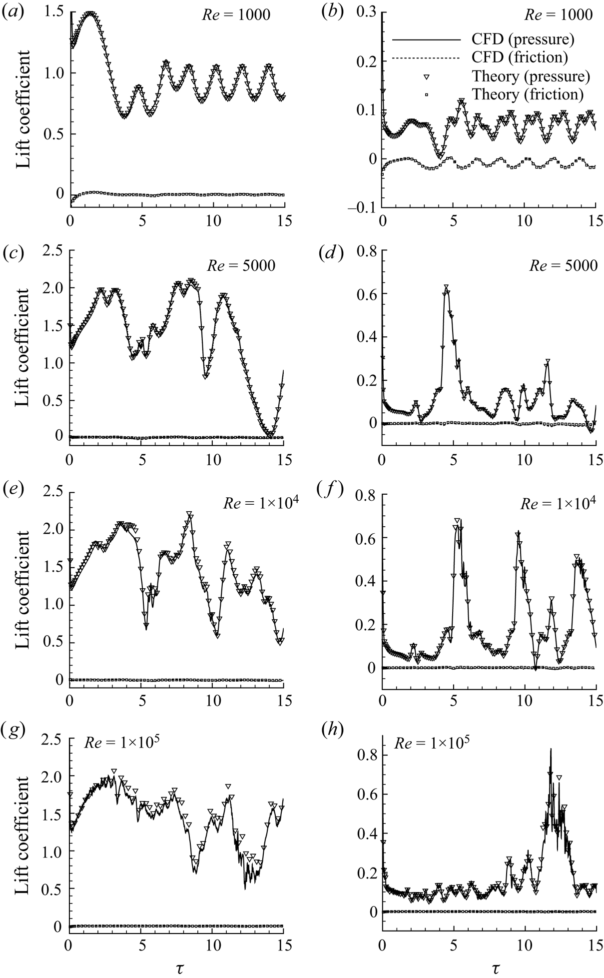
Figure 6. Comparison between theory and CFD for time-dependent lift coefficients for wing–flap configuration with deflection angle of flap  $ \delta =0^{\circ }$ for $ \alpha =20^{\circ }$ at $Re=1000$, $5000$, $1\times 10^4$ and $1\times 10^5$: (a,c,e,g) main aerofoil; (b,d, f,h) flap. Note that the dotted ‘CFD (friction)’ lines are lost behind the symbols for ‘Theory (friction)’, which indicates a good fit between the proposed formula and the CFD calculation.
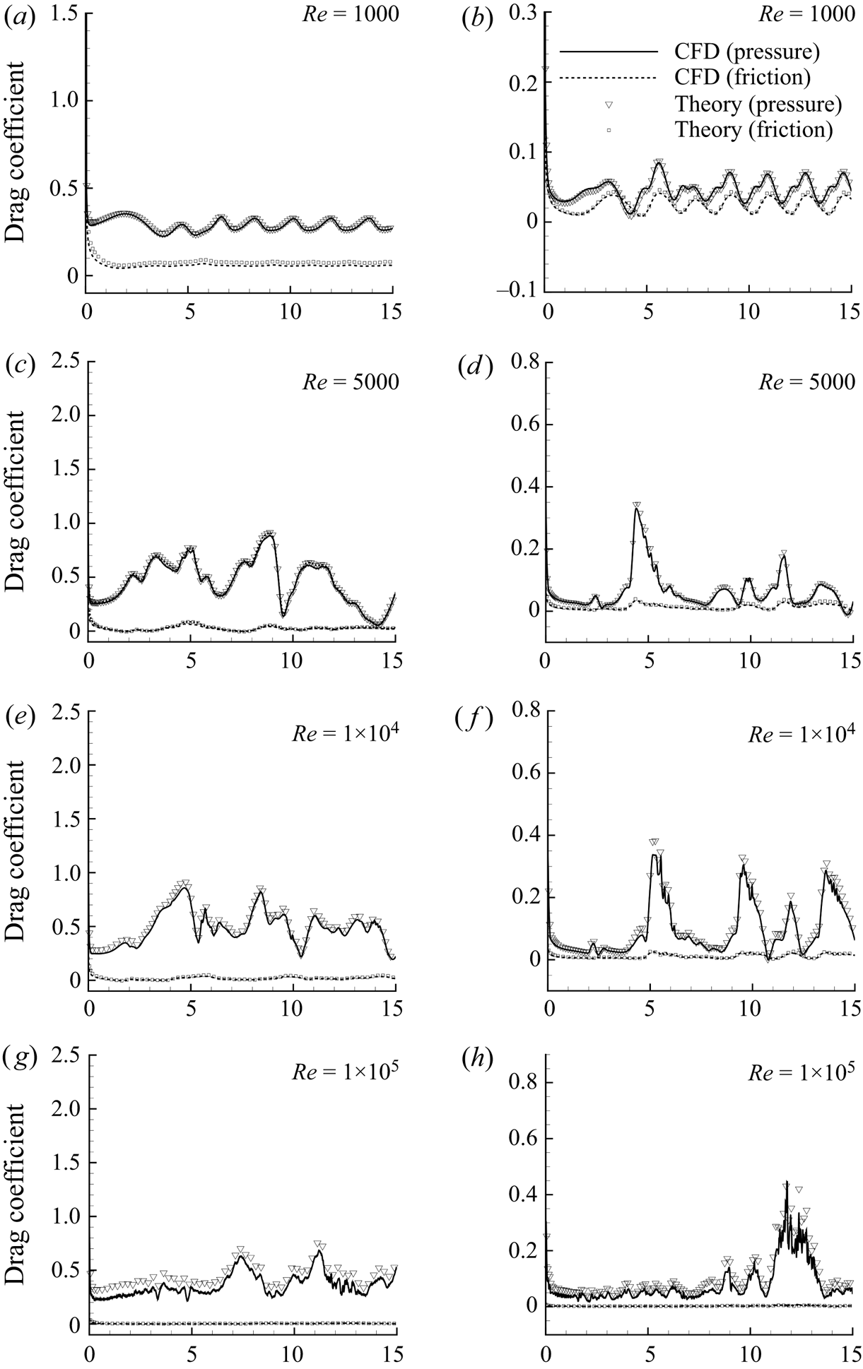
Figure 7. Comparison between theory and CFD for time-dependent drag coefficients for wing–flap configuration with deflection angle of flap  $ \delta =0^{\circ }$ for $ \alpha =20^{\circ }$ at $Re=1000$, $5000$, $1\times 10^4$ and $1\times 10^5$: (a,c,e,g) main aerofoil; (b,d, f,h) flap. Note that the dotted ‘CFD (friction)’ lines are lost behind the symbols for ‘Theory (friction)’, which indicates a good fit between the proposed formula and the CFD calculation.
The pressure forces (lift and drag) for both the main aerofoil and the flap are singular at the initial moment, as the added mass force term in the pressure force is infinite, as discussed above, and the vortex-pressure force term is also infinite due to an abrupt change in the body surface vorticity. When the Reynolds number is low (say  ${Re}=1000$), the force curves show periodic oscillation at a large time ( $\tau \geq 8$). When the Reynolds number is large enough ( ${Re}\geq 1\times 10^4$), the friction forces are close to $0$ and the pressure forces show some small amplitude oscillation related to the generation and movement of small vortices.
4.2.2. Vortex lift and drag for different deflection angles of flap
Good comparisons are also found between theory and CFD for wing–flap configurations with  $\delta =\pm 20^{\circ }$ for fixed angle of attack $\alpha =20^{\circ }$ and Reynolds number ${Re}=1\times 10^4$, as shown in figure 8 for lift and figure 9 for drag. It can be seen that the pressure force – summation of the forces contributed by a free vortex in the flow field (the vortex-pressure force) and the vorticity on the body surface (the viscous-pressure force) – is the dominant force, whereas the friction forces are minor. The pressure forces (both lift and drag) for $\delta =20^{\circ }$ are significantly larger than those for $\delta =-20^{\circ }$.

Figure 8. Comparison between theory and CFD for time-dependent lift coefficients for wing–flap configurations with deflection angles of flap  $ \delta =\pm 20^{\circ }$ for $ \alpha =20^{\circ }$ at $Re=1\times 10^4$: (a,c) main aerofoil; (b,d) flap. Note that the dotted ‘CFD (friction)’ lines are lost behind the symbols for ‘Theory (friction)’, which indicates a good fit between the proposed formula and the CFD calculation.
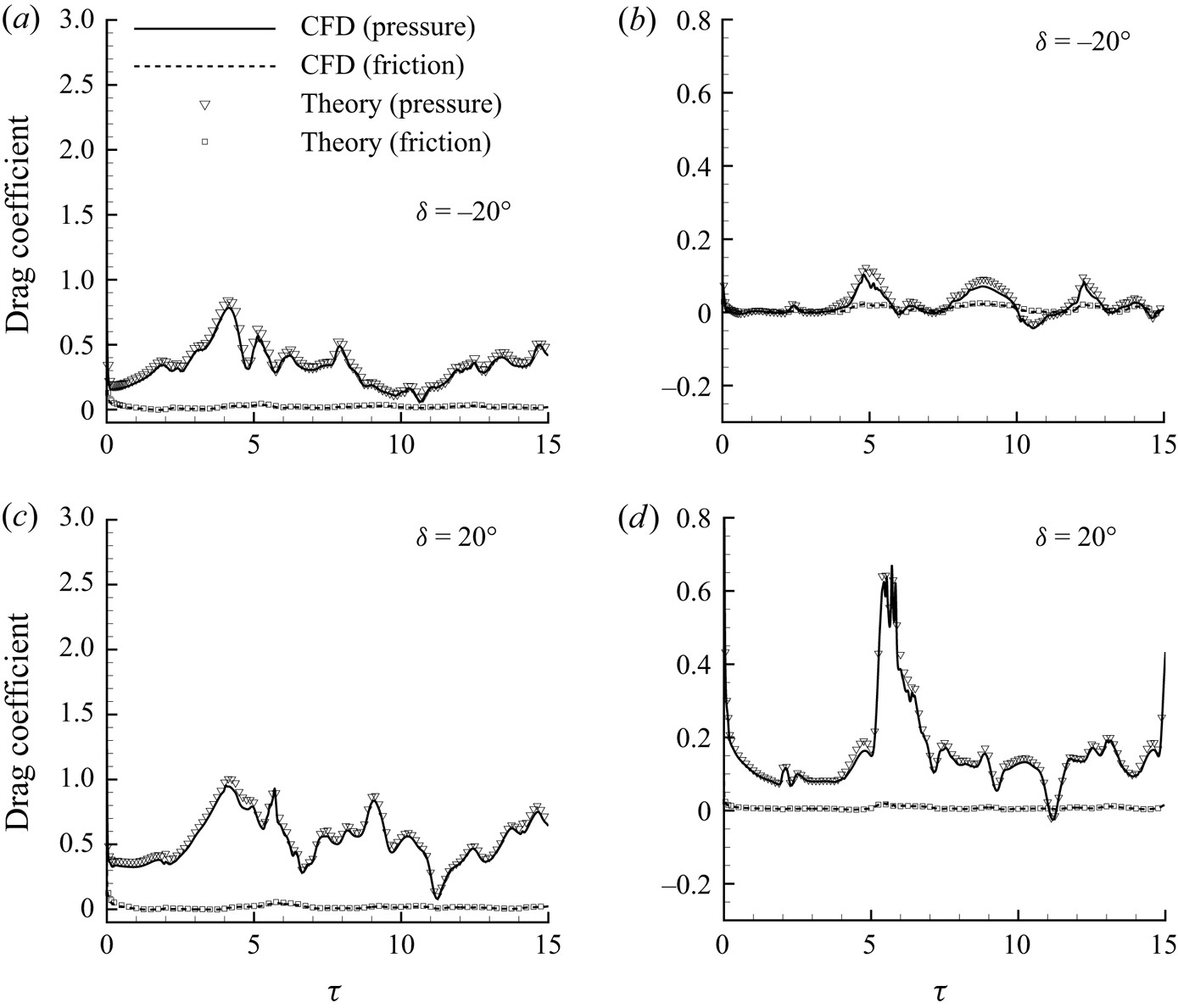
Figure 9. Comparison between theory and CFD for time-dependent drag coefficients for wing–flap configurations with deflection angles of flap  $ \delta =\pm 20^{\circ }$ for $ \alpha =20^{\circ }$ at $Re=1\times 10^4$: (a,c) main aerofoil; (b,d) flap. Note that the dotted ‘CFD (friction)’ lines are lost behind the symbols for ‘Theory (friction)’, which indicates a good fit between the proposed formula and the CFD calculation.
4.2.3. Vortex lift and drag for different angles of attack
To demonstrate the validity of the proposed vortex force method for different angles of attack, the comparisons between theory and CFD results for a wing–flap configuration with  $\delta =0^{\circ }$ and for ${Re}=1000$ at $\alpha =45^{\circ }$ and $60^{\circ }$ are shown in figure 10 for lift and in figure 11 for drag. The comparisons agree well. The force curves show periodicity in these cases, and the period lengths for the main aerofoil and the flap are equal at the same angle of attack. The force oscillating behaviour related to the vortex evolution in the flow field will be discussed in § 4.3.

Figure 10. Comparison between theory and CFD for time-dependent lift coefficients for wing–flap configuration with  $0^{\circ }$ deflection angle of flap at $Re=1000$: (a) main aerofoil at $ \alpha =45^{\circ }$; (b) flap at $ \alpha =45^{\circ }$; (c) main aerofoil at $ \alpha =60^{\circ }$; (d) flap at $ \alpha =60^{\circ }$. Note that the dotted ‘CFD (friction)’ lines are lost behind the symbols for ‘Theory (friction)’, which indicates a good fit between the proposed formula and the CFD calculation.

Figure 11. Comparison between theory and CFD for time-dependent drag coefficients for wing–flap configuration with  $0^{\circ }$ deflection angle of flap at $Re=1000$: (a) main aerofoil at $ \alpha =45^{\circ }$; (b) flap at $ \alpha =45^{\circ }$; (c) main aerofoil at $ \alpha =60^{\circ }$; (d) flap at $ \alpha =60^{\circ }$. Note that the dotted ‘CFD (friction)’ lines are lost behind the symbols for ‘Theory (friction)’, which indicates a good fit between the proposed formula and the CFD calculation.
4.3. Vortex force analysis
In this subsection, the evolution of three force components (the vortex-pressure force, the viscous-pressure force and the skin-friction force) acting on both the main aerofoil and the flap are studied. The relationship between the variation of the dominant force (the vortex-pressure force) against time and the change of vortex flow structures is analysed. The example case of lift forces acting on an impulsively started wing–flap configuration with  $\delta =0^{\circ }$ at $\alpha =45^{\circ }$, ${Re}=1000$ is presented here. The lift and drag results for other cases, at different angles of attack, different Reynolds numbers, and with different deflection angles, can be analysed in a similar way.
4.3.1. Analysis of different force components
The evolution of the total lift coefficients and their three components for both the main aerofoil and the flap in a wing–flap configuration is shown in figure 12, together with the vorticity field and streamlines at typical instants:  $\tau _{0}=0.125$, $\tau _{i}=i$ ( $i=1,2,\ldots,8$). It can be seen from the figure that for both the mainaerofoil and the flap, the oscillating behaviour of total lift coefficients is almost the same as that of vortex-pressure lift. Moreover, the summation of the viscous-pressure lift and the skin-friction lift on the main aerofoil is about 0.2, and the summation of those two lift components on the flap is close to zero. In other words, the dominant forces are the vortex-pressure forces. The oscillatory force curves for all the components exhibit periodicity in the considered case, and the non-dimensional period is equal to roughly $4$.
$4$.
4.3.2. Analysis of force oscillation related to vortex structures
It can be seen from figure 12 that the force variation has a close relationship with the evolution of vortex structure in the flow field, which is a reflection of the definition of the dominant force (i.e. the vortex-pressure force): the integration of the scalar product of the local vortex force vector and velocity multiplied by vortex strength.

Figure 12. Vortex lift evolution for an impulsively started wing–flap configuration with  $0^{\circ }$ deflection angle of flap for $ \alpha =45^{\circ }$ at $Re=1000$: (a) main aerofoil; (b) flap. The total force as well as its three components are shown here. The vorticity distribution and streamlines at typical instants are also given.
To demonstrate this relationship, we select one complete period of vortex-shedding. For the main aerofoil, the lift experiences periodic oscillation with four stages: the LEV-augmentation stage; the high-level force plateau stage; the force drop stage; and the low-level force plateau stage. These four stages can be observed in figure 12(a). In the LEV-augmentation stage (from  $\tau = 0$ to $\tau = 1$ and from $\tau = 4.5$ to $\tau = 5.5$), a clockwise LEV is expanding and convecting above the upper surface of the main aerofoil. In the high-level force plateau stage (e.g. from $\tau = 5.5$ to $\tau = 6.5$), the earlier TEV moves downstream far from the body, and a newly generated TEV is forming. In the force drop stage (from $\tau = 1$ to $\tau = 3$, and from $\tau = 6.5$ to $\tau = 7.5$), the main clockwise LEV and counterclockwise TEV are released and moving far away from the surface; in the meantime, a new pair of secondary LEV and a new TEV are developing at the leading edge and trailing edge, respectively. In the low-level force plateau stage (from $\tau = 3$ to $\tau = 4.5$, and from $\tau = 7.5$ to $\tau = 9$), the secondary LEV pair and the newly formed TEV are expanding. These gradually occupy the whole area of the upper surface and interact with each other.
The spatial distribution of local vortex-pressure lift due to the local vorticity at  $8$ typical instants $\tau _{i}=i$ ( $i=1,2,\ldots,8$) for the two bodies involved (the main aerofoil and the flap) are shown in figures 13 and 14. Figure 13 is for instants $\tau _{i}=i$ with $i=1,2,3,4$, and figure 14 is for instants $\tau _{i}=i$ with $i=5,6,7,8$. Figures 13(a) and 14(a) are for the lift acting on the main aerofoil, and figures 13(b) and 14(b) are for the lift acting on the flap. The theoretical vortex-pressure lift coefficients on either the main aerofoil or the flap are obtained by summing the lift coefficients of vortices inside all grid cells. We can see clearly that the lift-contributing areas for both the main aerofoil and the flap lie in an area close to the upper surface of the body. It is also observed that the force variation is highly related to the vortical flow structure.

Figure 13. Contours of vortex lift distribution displaying lift coefficients acting on (a) main aerofoil and (b) flap, contributed by local vortices, for a wing–flap configuration starting flow at instants  $ \tau =1,2,3,4$, with streamlines showing the vortex structure.

Figure 14. Contours of vortex lift distribution displaying lift coefficients acting on (a) main aerofoil and (b) flap, contributed by local vortices, for a wing–flap configuration starting flow at instants  $ \tau =5,6,7,8$, with streamlines showing the vortex structure.
Relating figures 13(a) and 14(a) to figure 12 allows us to analyse how the evolution of vortical structures in the flow field influence the lift acting on the main aerofoil.
(i) The LEV-augmentation stage (e.g. from
${\tau = 0}$ to ${\tau = 1}$, and from ${\tau = 4.5}$ to ${\tau = 5.5}$) is caused by the growth of the main LEV above the upper surface of the main aerofoil, resulting in a low-pressure suction area above the leading edge.(ii) The large force in the high-level force equilibrium stage (e.g. from
${\tau = 5.5}$ to ${\tau = 6.5}$) is due to an offset between the release of the LEV lift-augmentation effect and the TEV lift-increasing effect.(iii) The force drop in the next stage (e.g. from
${\tau = 1}$ to ${\tau = 3}$, and from ${\tau = 6.5}$ to ${\tau = 7.5}$) is owing to the newly formed LEV vortex pair squeezing away the main LEV that originally contributed to the large lift force. Moreover, the newly generated TEV also causes a large lift drop due to its downwash effect.(iv) In the low-level force equilibrium stage (e.g. from
${\tau = 3}$ to ${\tau = 4.5}$, and from ${\tau = 7.5}$ to ${\tau = 9}$), the lift keeps at a relatively low stable value with a slight increase because of the growth of the secondary LEV pair and the TEV moving upstream to the upper surface.


The lift on the flap could be analysed in a similar way. Unlike the lift acting on the main aerofoil, the lift acting on the flap exhibits three stages in one period: the lift-reduction stage, the stable stage, and the lift-increase stage, which can be observed in figure 12(b). During the lift-reduction stage (e.g. from  ${\tau = 0}$ to ${\tau = 0.2}$, and from $\tau =3.8$ to $\tau =5$), the TEV is blown away from the upper surface of the flap. In the stable stage (e.g. from $\tau = 1$ to $\tau = 3$, and from $\tau = 5$ to $\tau = 7$), the lift maintains a stable, low value, and the flow field consists of a complex interaction of the main and secondary LEV and TEV. After that is the lift-increase stage (e.g. from $\tau = 3$ to $\tau = 3.8$, and from $\tau =7$ to $\tau =7.8$) when the TEV generated in the last stage moves upstream to the upper surface of the flap. Figures 13(b) and 14(b) show the spatial distribution of local vortex-pressure lift due to vortices inside each grid cell at eight typical instants $\tau _{i}=i$ ( $i=1,2,\ldots,8$) for the flap. We can see from these figures that the lift on the flap is caused mainly by the main LEV and TEV as well as the vortex sheet in the boundary layer, while the secondary vortex structures contribute little lift to the flap.
Combining the vortex lift distribution in figures 13(b) and 14(b) with figure 12, we could analyse how the evolution of vortical structures in the flow field influences the lift acting on the flap.
(i) The flap lift-decrease stage is related to the collapse of the suction effect with blowing away of the TEV on the upper surface of the flap.
(ii) The stable stage is due to the newly formed TEV contributing to positive lift, which compensates for the lift loss.
(iii) The flap lift-increase stage could be explained by the suction mechanism caused by the growth of the TEV.
It is also interesting to compare these images to the single-body simulation in Li et al. (Reference Li, Wang, Graham and Zhao2021), figure 10. One can notice a very significant reduction in the contribution from the TEV shed after the initial transient (evident at e.g.  $\tau = 4{-}6$ s) to the lift on the main body compared to a single-body case, despite body 1 taking up almost 90 % of the entire chord. Meanwhile, the influences of both the LEV and the TEV on the second body (trailing-edge body) are equally profound.
5. Summary
In this paper, the vortex force approach for viscous flows for multi-bodies has been developed. The lift and drag forces for each individual body in a multi-body configuration have been derived, with both pressure force (contributed by vorticity in the flow field and on the body surface) and viscous force included.
The pressure force contributed by vorticity in the flow field (also called vortex-pressure force) was found to be the dominant force and represented as the scalar product of the vortex-pressure force vector and the local flow velocity. The vortex-pressure force factors can be pre-computed by solving a Laplace equation. Vortex-pressure force maps for every individual body in the multi-body assembly were designed based on the vortex-pressure force factors for the purpose of identifying the force contribution of a given vortex in the flow field, and the positive and negative force-generating directions were defined in these maps. Flow control strategies could be designed to maintain or create the lift-enhancing/drag-reducing vortex and to minimize the lift-reducing/drag-increasing vortex according to the vortex-pressure force maps, where the force contribution of each given vortex could be analysed without pre-knowledge of the flow field. Another advantage of this VFM method for multi-bodies is its capability to extract force from limited/low-resolution flow data, e.g. PIV fields, in a non-invasive manner.
In order to illustrate the proposed vortex force decomposition method, analyses have been made for an unsteady flow around wing–flap configurations. The force predictions arising from the current vortex force method have been shown to agree satisfactorily with those from CFD simulations. For both the main aerofoil and the flap, we found that the dominant force was the vortex-pressure force. When the Reynolds number was large enough (greater than  $1000$), the pressure force contributed by the newly created vorticity on the body surface and the skin-friction force are negligible. The force oscillation behaviour, as well as its relationship with the vortex flow pattern and vortex-pressure force map, have also been studied. The study of the spatial distribution of local vortex force due to vortices inside each grid cell provided additional evidence for those correlations. And it has been shown that the force acting on both the main aerofoil and the flap is closely related to the vortex evolution near the wing–flap configuration. The spatial distribution of the vortex-pressure force analysis on the main aerofoil showed that the four force stages – the LEV-augmentation stage, the high-level force equilibrium stage, the force drop stage and the low-level force equilibrium stage – were highly related to the evolution of the vortical structures. Similarly, the analysis of the spatial distribution of the vortex-pressure force on the flap showed the influence of the vortical structures on the three-stage force oscillation: the flap force increase stage was due to the collapse of the LEV suction; the force stable stage was due to a balance between the TEV force-enhancing effect and the suction loss of the LEV; and the force increase stage was a result of the TEV suction effect.
In summary, we presented a force decomposition method for incompressible unsteady viscous flows applicable to a wide range of Reynolds numbers. We have shown that the concept of vortex-pressure maps still exists for individual bodies when the flow field contains multiple bodies, and that their form should not be understood as superposition from individual contributions. As an application, two-dimensional results of a wing–flap starting flow agreed well with CFD results. The theoretical appeal of this method lies in: (i) separating the body forces and providing links to the flow features (velocity and vorticity), which provides a better understanding of the origin of aerodynamic and hydrodynamic forces; (ii) obtaining force directly from the velocity field near the bodies. The method presented here can also be extended easily to the study of vortex torque as future work.
Funding
This work has received funding from the European Union's Horizon 2020 research and innovation programme under the Marie Sklodowska-Curie grant agreement no. 765579. The work was also funded by the Leverhulme Trust, Grant ref. ECF-2018-727. Their support is gratefully acknowledged.
Declaration of interests
The authors report no conflict of interest.


 Open access