


1. Introduction
Optimisation of combustion efficiency and energy conversion calls for high-pressure combustion chambers. Diesel and gas turbines may operate in the range of 20–60 bar, whereas rocket engines can reach much higher pressures of between 70 and 200 bar. Typical fuels used in these applications are liquid hydrocarbon mixtures of n-octane, n-decane and n-dodecane, among other components, which have critical pressures around 20 bar. Therefore, operating conditions with near-critical or supercritical pressures for the fuel are common. Experimental studies at these extreme pressures reveal a thermodynamic transition where the distinction between liquid and gas is lost. The sharp phase interface is immersed in a variable-density layer with similar liquid and gas properties, and is rapidly distorted by hydrodynamic instabilities and turbulence (Mayer & Tamura Reference Mayer and Tamura1996; Mayer et al. Reference Mayer, Schik, Vielle, Chauveau, Gökalp, Talley and Woodward1998, Reference Mayer, Schik, Schaffler and Tamura2000; Oschwald et al. Reference Oschwald, Smith, Branam, Hussong, Schik, Chehroudi and Talley2006; Chehroudi Reference Chehroudi2012; Falgout et al. Reference Falgout, Rahm, Sedarsky and Linne2016; Crua, Manin & Pickett Reference Crua, Manin and Pickett2017). In the past, a description of these observations was given as a sudden transition from a liquid to a gas-like supercritical state (Spalding Reference Spalding1959; Rosner Reference Rosner1967). However, the requirement that liquid and gas be in local thermodynamic equilibrium (LTE) at the interface provides evidence that a two-phase transcritical behaviour exists within a specific region of the mixture thermodynamic space. That is, the pressure is supercritical for the pure fluid but the temperature and pressure are below the mixture critical-point values. LTE enhances the solubility of the ambient gas into the liquid fuel, which causes a local change in mixture critical properties and the growth of mixing layers with significant variations of fluid properties in each phase (Poblador-Ibanez & Sirignano Reference Poblador-Ibanez and Sirignano2018; Davis, Poblador-Ibanez & Sirignano Reference Davis, Poblador-Ibanez and Sirignano2021; Poblador-Ibanez, Davis & Sirignano Reference Poblador-Ibanez, Davis and Sirignano2021).
This definition of transcritical conditions follows from previous literature focusing on transcritical droplet vaporisation at supercritical pressures (Hsieh, Shuen & Yang Reference Hsieh, Shuen and Yang1991; Delplanque & Sirignano Reference Delplanque and Sirignano1993; Yang & Shuen Reference Yang and Shuen1994; Delplanque & Sirignano Reference Delplanque and Sirignano1995, Reference Delplanque and Sirignano1996). However, this differs from other authors who define transcritical conditions as the transition from a liquid-like to a gas-like fluid behaviour across the pseudo-boiling or Widom line at supercritical conditions (Lapenna Reference Lapenna2018; Kawai Reference Kawai2019; Lagarza-Cortés et al. Reference Lagarza-Cortés, Ramírez-Cruz, Salinas-Vázquez, Vicente-Rodríguez and Cubos-Ramírez2019; Bernades, Capuano & Jofre Reference Bernades, Capuano and Jofre2023). Thus, these refer to the large nonlinear variations of fluid properties within a specific temperature range rather than the existence of two distinct phases separated by a sharp interface.
The phase-equilibrium assumption cannot apply beyond the mixture critical point where the two-phase interface transitions to a supercritical diffuse mixing between liquid-like and gas-like states. Other limitations of LTE have been discussed in the literature. LTE breaks down when large interfacial thermal resistivity exists and the temperature jump across the phase non-equilibrium layer cannot be neglected (Stierle et al. Reference Stierle, Waibel, Gross, Steinhausen, Weigand and Lamanna2020). In addition, Dahms & Oefelein (Reference Dahms and Oefelein2013, Reference Dahms and Oefelein2015a,Reference Dahms and Oefeleinb) and Dahms (Reference Dahms2016) discussed and quantified the interface internal structure transition to the continuum domain at transcritical conditions. At temperatures near the mixture critical temperature and at very high pressures, the interfacial transition region may enter a continuum, with LTE no longer being a good modelling choice. It must be understood that the thermodynamic equilibrium of the continuous fluid is maintained throughout the layer; there is no question about the equation of state. However, the distinction between the two phases has disappeared and disallowed the use of the phase-equilibrium law. For interface temperatures sufficiently below the mixture critical temperature at a given pressure, LTE is well established. Mixing regions grow rapidly in the order of micrometres whereas the thickness of the interfacial region remains in the nanoscale. The temperature jump across the interface and the phase transition thickness become negligible; thus, the interface can be considered a sharp discontinuity with a jump in fluid properties (Poblador-Ibanez & Sirignano Reference Poblador-Ibanez and Sirignano2018; Davis et al. Reference Davis, Poblador-Ibanez and Sirignano2021). For practical purposes, the non-equilibrium layer of compressive shocks is treated as a discontinuity, despite its thickness being at least an order of magnitude greater than the phase non-equilibrium transition region. Additional details on the behaviour of transcritical interfaces are provided in Jofre & Urzay (Reference Jofre and Urzay2021), who review, e.g. equilibrium and non-equilibrium formulations or the stability mechanisms determining whether transcritical interfaces arise.
The described physics explain why experimental observations have trouble capturing a two-phase environment. LTE drives the liquid and gas phases to be more alike near the interface. That is, the composition, density and viscosity of both fluids become similar (e.g. the gas phase becomes denser and the liquid viscosity drops to gas-like values) (Yang Reference Yang2000; Poblador-Ibanez & Sirignano Reference Poblador-Ibanez and Sirignano2018, Reference Poblador-Ibanez and Sirignano2022a). As a result, surface tension decreases substantially and vanishes at the mixture critical point. Therefore, the interface may experience a fast growth of short-wavelength surface perturbations, resulting in the early breakup into small ligaments and droplets and a mixing enhancement (Poblador-Ibanez & Sirignano Reference Poblador-Ibanez and Sirignano2021). In fact, surface tension is oftentimes neglected in the literature under the assumption that the transcritical interfacial region is diffusion-driven. This approach is usually motivated by mesh resolution constraints in capturing such small structures in a system-sized domain and loses detailed information on the atomisation process and droplet characteristics, e.g. diameter and distribution (Matheis & Hickel Reference Matheis and Hickel2018; Koukouvinis et al. Reference Koukouvinis, Vidal-Roncero, Rodriguez, Gavaises and Pickett2020; Yang, Yi & Habchi Reference Yang, Yi and Habchi2020; Fathi, Hickel & Roekaerts Reference Fathi, Hickel and Roekaerts2022). Nonetheless, some authors have addressed the development of sub-grid models to obtain the transcritical spray characteristics using similar numerical frameworks (Gaballa, Habchi & de Hemptinne Reference Gaballa, Habchi and de Hemptinne2023).
Numerical studies have become necessary to understand in detail the atomisation process of liquid jets and improve the design of atomisers to enhance spray formation and fuel–oxidiser mixing. Such analyses are common for incompressible flows, e.g. the temporal studies of round jets and planar jets by Jarrahbashi & Sirignano (Reference Jarrahbashi and Sirignano2014), Jarrahbashi et al. (Reference Jarrahbashi, Sirignano, Popov and Hussain2016) and Zandian, Sirignano & Hussain (Reference Zandian, Sirignano and Hussain2017, Reference Zandian, Sirignano and Hussain2018, Reference Zandian, Sirignano and Hussain2019a,Reference Zandian, Sirignano and Hussainb). The novelty introduced by these authors is the inclusion of vorticity dynamics to explain the atomisation cascade process of liquid structures as a result of the interactions between hairpin vortices and Kelvin–Helmholtz (KH) vortices. Previous works have used vorticity dynamics to understand how vortex stretching, tilting and baroclinicity relate to the generation of three-dimensional perturbations leading to atomisation in incompressible flows. A detailed literature review is provided in Jarrahbashi & Sirignano (Reference Jarrahbashi and Sirignano2014), Jarrahbashi et al. (Reference Jarrahbashi, Sirignano, Popov and Hussain2016) and Zandian et al. (Reference Zandian, Sirignano and Hussain2018). More recently, Zandian et al. (Reference Zandian, Sirignano and Hussain2019b) extended the detailed analysis of vortex interactions to spatially-developing liquid jets submerged in a coaxial gas flow; Constante-Amores et al. (Reference Constante-Amores, Kahouadji, Batchvarov, Shin, Chergui, Juric and Matar2021) have shown how the transition between the capillary-controlled and inertia-controlled regimes leads to streamwise vorticity generation and hairpin vortex formation; and Gao et al. (Reference Gao, Chen, Qiu, Ding and Xie2022) have included phase change in their study of the atomisation of liquid round jets and have shown that droplet vaporisation has a substantial impact on the evolution and breakup of vortical structures. A reduction in droplets around the liquid core translates into a less-turbulent flow field where vortex rings deform into strip-shaped or streamwise vortices that remain unperturbed for longer times.
These works focus on shear-driven atomisation due to its fundamental importance in power and propulsion applications. As a result, vorticity dynamics are key in explaining the early deformation of the liquid jet into lobes, ligaments and droplets. Note that these studies address canonical configurations in nature due to the scope of their analyses; thus, other mechanisms that would enhance atomisation are usually not considered, such as the atomiser internal flow turbulence. Despite inducing different atomisation time scales and length scales, organised surface patterns (i.e. lobes) still develop and are arguably affected by the vorticity dynamics (Agarwal & Trujillo Reference Agarwal and Trujillo2020). Significantly, Zandian et al. (Reference Zandian, Sirignano and Hussain2017, Reference Zandian, Sirignano and Hussain2018) classify the injection of planar liquid jets using a liquid Reynolds number, 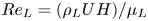 $Re_L =(\rho _LUH)/\mu _L$, and a gas Weber number,
 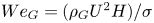 ${We}_G =(\rho _GU^2H)/\sigma$, where
  $\rho _L$ and
  $\rho _G$ are the liquid and gas freestream densities,
  $\mu _L$ the liquid viscosity,
  $U$ the relative velocity between gas and liquid streams,
  $H$ the jet thickness and
  $\sigma$ the surface-tension coefficient. Using
  ${We}_G$, the effects of the density ratio,
  $\rho _G/\rho _L$, are embedded in the classification (note that other works define the density ratio as
  $\rho _L/\rho _G$). Under this set of parameters, three atomisation sub-domains are identified according to the deformation cascade: (a) the lobe–ligament–droplet (LoLiD) sub-domain characterised by low
  $Re_L$ and
  ${We}_G$ with the formation and stretching of lobes, which eventually break up into large droplets due to capillary instabilities; (b) the lobe–hole–bridge–ligament–droplet (LoHBrLiD) sub-domain characterised by higher inertia forces compared to surface tension (i.e. higher gas density or lower surface-tension coefficient). Lobes are easily perforated by the gas phase, with holes expanding and forming bridges that eventually break off into ligaments and droplets; and (c) the lobe–corrugation–ligament–droplet (LoCLiD) similar to LoLiD, but where higher Reynolds numbers generate lobes that develop small-scale corrugations near the edge, forming smaller ligaments and droplets. Figure 1(a) summarises this classification in a
  ${We}_G$ vs
  $Re_L$ diagram, highlighting the transition regions between the sub-domains. Below
  ${We}_G<4900$, the LoLiD sub-domain transitions into the LoCLiD sub-domain around
  $Re_L\approx 2500$, whereas the boundary of the LoHBrLiD sub-domain is defined by a best-fit curve linking two different transition trends (Zandian et al. Reference Zandian, Sirignano and Hussain2017). At low
  $Re_L$, the transitional boundary follows a hyperbolic relation (i.e.
 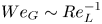 ${We}_G\sim Re_L^{-1}$), but at higher
  $Re_L$ a parabolic trend emerges defined by a modified Ohnesorge number that includes the density ratio,
  ${Oh}_m=\sqrt {{We}_G}/Re_L=\sqrt {\rho _G/\rho _L}{Oh}\approx 0.021$. As reported in Zandian et al. (Reference Zandian, Sirignano and Hussain2017), this classification is fairly generic and independent of the liquid jet geometry when compared with other works, e.g. Desjardins & Pitsch (Reference Desjardins and Pitsch2010), Shinjo & Umemura (Reference Shinjo and Umemura2010), Herrmann (Reference Herrmann2011) and Jarrahbashi et al. (Reference Jarrahbashi, Sirignano, Popov and Hussain2016).

Figure 1. Classification of atomisation sub-domains and breakup features in a gas Weber number,  ${We}_G$, vs liquid Reynolds number,
  $Re_L$, diagram: (a) incompressible framework described by Zandian et al. (Reference Zandian, Sirignano and Hussain2017); and (b) transcritical work by PS. Also shown are the transcritical configurations from PS listed in table 1.
The results from these incompressible studies indicate that very fast atomisation with the generation of small liquid structures occurs in real-engine configurations where gas inertia becomes important and surface-tension forces decrease. However, they fail to incorporate the detailed physics and real-fluid thermodynamics characteristic of the atomisation of liquid fuels at engine-relevant conditions and, therefore, are more representative of subcritical environments. Moreover, the configuration parametrisation by varying  $U$,
$U$,  $H$,
$H$,  $Re_L$,
  ${We}_G$, the density ratio and the viscosity ratio might result in fluid properties not representative of the real fluids in typical combustion applications if care is not taken. Comprehending the early mixing process and atomisation in real-engine configurations prior to the eventual liquid mixture heating, vaporisation and possible shift to a supercritical state requires examining the fast surface deformation processes under transcritical conditions.
Following these works, Poblador-Ibanez & Sirignano (Reference Poblador-Ibanez and Sirignano2022a) (hereafter PS) performed a temporal analysis of a three-dimensional planar liquid n-decane jet submerged in a hotter gaseous oxygen stream at transcritical conditions. Various ambient pressures are considered well above the critical pressure of n-decane while a two-phase interface is sustained. They showed the influence of intraphase mixing, reduced surface tension and varying interface properties on the early deformation of the transcritical jet. A primary deformation mechanism arises at very high pressures (i.e. above 100 bar) as a direct result of the transcritical thermodynamics. The production of large ligaments and droplets is suppressed, and the liquid deforms in a gas-like manner with continuous stretching, folding and layering of liquid sheets. Only localised mixing may cause the growth of short-wavelength perturbations that generate sub-micrometre ligaments and droplets. That is, certain liquid regions can become unstable if the liquid viscosity and surface tension drop. Apart from the layering mechanism, breakup patterns similar to those identified in the incompressible sub-domains LoHBrLiD or LoCLiD may occur at much lower  $Re_L$ and
  ${We}_G$ as a direct result of the variation of fluid properties within each phase and the reduced surface tension as the ambient pressure increases. The shear across the initially perturbed phase interface generates early lobes that evolve differently depending on the problem configuration. For
  ${We}_G <1000$, a lobe bending mechanism occurs whereby lobes stretch, thin and easily bend toward the oxidiser stream before being perforated at very high pressures. In contrast, higher
  ${We}_G$ modify the deformation pattern with lobes corrugating around the streamwise direction before bursting into droplets, resembling a bag-breakup mechanism. In summary, higher pressures promote gas-like turbulent mixing with frequent hole formation. These transcritical effects observed in the n-decane/oxygen mixture are shown in figure 1(b), where the transition between lobe bending and corrugation mechanisms, as well as evidence of layering, are presented. For each pressure, a curve is obtained in the
  ${We}_G$ vs
  $Re_L$ diagram by fixing the properties of both fluids and the jet thickness, while varying the relative velocity
  $U$. Note that figure 1 shows the classification of the cases analysed in PS (i.e. A1, A2, B1, B2, C1, C2 and C3) in the
  ${We}_G$ vs
  $Re_L$ diagrams representative of the incompressible framework and the transcritical framework. These configurations are introduced in § 2 and summarised in table 1. A visualisation of the planar jet deformation process in case C2 is also given in § 2 (see figure 3).
Table 1. List of analysed cases from PS using liquid n-decane at 450 K and gaseous oxygen at 550 K. The subscripts  $G$ and
  $L$ refer to freestream conditions for the gas and the liquid phases.

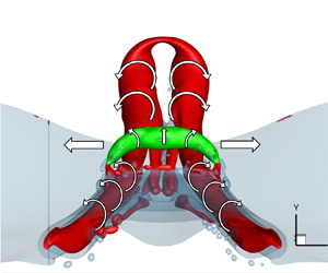
Beyond identifying distinct deformation patterns at transcritical conditions, PS also provide a comprehensive discussion on surface instability triggers, the effects of intraphase mixing and the subsequent change in fluid properties, quantify the breakup of ligaments and droplets and analyse the varying interface thermodynamic state and mass exchange. However, the new focus of this work is on studying the vorticity dynamics to explain how the deformation mechanisms identified by PS result from vortical motion. The gas-like behaviour of the liquid phase near the interface suggests that vortex-related surface deformation is stronger than seen in previous incompressible studies. Note that vorticity dynamics are also considered in studies of jets injected into conditions ranging from transcritical to supercritical environments. Usually, such works focus on the breakup of the primary vortical structures (e.g. rings or rollers) into smaller vortices as a measure of the atomisation or turbulent mixing onset and to describe flow patterns (Gnanaskandan & Bellan Reference Gnanaskandan and Bellan2018; Lagarza-Cortés et al. Reference Lagarza-Cortés, Ramírez-Cruz, Salinas-Vázquez, Vicente-Rodríguez and Cubos-Ramírez2019; Wang, Wang & Yang Reference Wang, Wang and Yang2019; Koukouvinis et al. Reference Koukouvinis, Vidal-Roncero, Rodriguez, Gavaises and Pickett2020). However, such studies either neglect or do not involve surface tension, and little to no emphasis is given to the complex interaction between vorticity and liquid atomisation. Therefore, the data from PS can provide evidence of the competition between surface tension, diffusion processes and shear for a range of transcritical conditions.
For this study, we take the configurations of PS and post-process the data to identify the vortical features using the vortex identification method  $\lambda _\rho$ by Yao & Hussain (Reference Yao and Hussain2018). The goal here is to establish a clear connection between the deformation of transcritical jets and vorticity dynamics, similar to Zandian et al. (Reference Zandian, Sirignano and Hussain2017, Reference Zandian, Sirignano and Hussain2018). The
  $\lambda _\rho$ method is a compressible extension of the incompressible
  $\lambda _2$ method of Jeong & Hussain (Reference Jeong and Hussain1995) and it has been chosen in favour of another widely-used vortex identification method, the Q-criterion (Hunt, Wray & Moin Reference Hunt, Wray and Moin1988). The Q-criterion may be inconsistent for vortices subject to strong external strain, such as in liquid atomisation, and has an ambiguous extension to compressible flows. On the other hand,
  $\lambda _2$ or
  $\lambda _\rho$ are more suitable for this type of flows (Kolář Reference Kolář2007). For example,
  $\lambda _2$ has already been shown successful in identifying vortex structures in multiphase flow computations and establishing a link between their evolution and surface dynamics (Zandian et al. Reference Zandian, Sirignano and Hussain2018, Reference Zandian, Sirignano and Hussain2019b; Gao et al. Reference Gao, Chen, Qiu, Ding and Xie2022).
This paper is structured as follows. First, § 2 describes the transcritical configurations of PS (e.g. selected species, temperature, pressure, computational domain). Then, § 3 summarises the physical modelling and numerical techniques used in the computations, for which a detailed description can be found in Poblador-Ibanez & Sirignano (Reference Poblador-Ibanez and Sirignano2022b). The vortex identification method  $\lambda _\rho$ of Yao & Hussain (Reference Yao and Hussain2018) is reviewed in § 4, and best practices are presented for its implementation in the post-processing of two-phase computations with a sharp interface. Section 5 presents selected post-processing of the simulations of PS, focusing on the liquid deformation by identifying vortical structures, as well as the vorticity generation mechanisms. Lastly, § 6 summarises the major findings and contributions of this work.
2. Flow configuration
The numerical study by PS considers a temporal analysis of a planar liquid n-decane jet initially at 450 K perturbed by a faster and hotter oxygen gaseous stream initially at 550 K. The hotter ambient gas provides enough energy to vaporise the fuel. Both species represent engines operating at high pressures with liquid hydrocarbon fuels injected into enriched air or pure oxygen. Under such conditions, both fluids might be supercritical away from the interface and the mixing layers. Therefore, the use of the terms ‘liquid’ and ‘gas’ to characterise each fluid might not be totally appropriate. However, we refer to the high-density, compressible fluid with n-decane as the dominant component as liquid, whether it is subcritical or supercritical locally. Likewise, the lower density fluid with oxygen as the major species is described as gas over the transcritical domain.
Various values for the gas freestream velocity,  $u_G$, and ambient pressure,
  $p_{amb}$, above the critical pressure of n-decane are considered (50, 100 and 150 bar). The critical pressures and critical temperatures of the analysed species are 21.03 bar and 617.70 K for n-decane and 50.43 bar and 154.58 K for oxygen. Thus, the ambient pressure is also supercritical for oxygen in some cases. Table 1 summarises the parameters for each configuration. All cases fall in a transcritical environment where a two-phase interface can be sustained with strong diffusive mixing surrounding it. For reference, figure 2 has been reproduced from PS to show the phase-equilibrium diagrams of the n-decane/oxygen binary mixture at various pressures, highlighting the domain of two-phase coexistence above the critical pressures of each species.

Figure 2. Phase-equilibrium diagrams obtained using the Soave–Redlich–Kwong (SRK) equation of state for the binary mixture of n-decane and oxygen. The mixture composition in each phase is represented by the mole fraction of n-decane as a function of temperature and pressure. The mixture critical point is shown. The figure is reproduced from PS.
A reduced computational domain is considered to limit the computational cost. Symmetry is imposed on the centre plane of the jet, periodic boundary conditions are used in the streamwise and spanwise directions and outflow boundary conditions are applied at the top gaseous boundary away from the phase interface. The jet thickness is  $H=20\ \mathrm {\mu }{\rm m}$ (i.e. only the half-thickness of
  $H'=10\ \mathrm {\mu }{\rm m}$ is included in the computational domain), and two initial streamwise (in
  $x$) and spanwise (in
  $z$) sinusoidal perturbations are superimposed on the jet's surface. The streamwise perturbation has a wavelength of
  $30\ \mathrm {\mu }{\rm m}$ and an amplitude of
  $0.5\ \mathrm {\mu }{\rm m}$; the spanwise perturbation has a wavelength of
  $20\ \mathrm {\mu }{\rm m}$ and an amplitude of
  $0.3\ \mathrm {\mu }{\rm m}$. The velocity field is initialised as
  $\boldsymbol {u}=(u(y),0,0)$, where
  $u(y)=(u_G/2)(\tanh {[6.5\times 10^{5}(y-H')]}+1)$, which distributes the streamwise velocity from
  $0\ {\rm m}\ {\rm s}^{-1}$ in the liquid phase to
  $u_G$ across the interface within a thin layer of about
  $6\ \mathrm {\mu }{\rm m}$. The initial instability is linear as the perturbation is sufficiently weak to let unstable waves evolve naturally. The perturbation along the spanwise direction is meant to accelerate the generation of three-dimensional flow structures. The initial wavelengths are chosen using estimates from Poblador-Ibanez & Sirignano (Reference Poblador-Ibanez and Sirignano2019) for an axisymmetric transcritical liquid jet. Guided by jet instability theory, the wavelengths are shorter than those used in incompressible studies where surface tension was generally stronger (i.e.
  $100\ \mathrm {\mu }{\rm m}$ in the studies by Zandian et al. (Reference Zandian, Sirignano and Hussain2017, Reference Zandian, Sirignano and Hussain2018)). Only one wavelength per direction is included in the numerical domain, with a size of
  $L_x=L_y=30 \ \mathrm {\mu }{\rm m}$ and
  $L_z=20\ \mathrm {\mu }{\rm m}$.
The domain is discretised with a Cartesian uniform mesh with  $450\times 450\times 300$ cells (i.e. a uniform mesh size of
  $\varDelta =0.0667\ \mathrm {\mu }{\rm m}$). A comprehensive summary of the physical and numerical modelling is provided in § 3 and is based on the work by Poblador-Ibanez & Sirignano (Reference Poblador-Ibanez and Sirignano2022b). There, the grid convergence properties of the model are discussed, showing the impact on the deformation and vaporisation of the liquid phase. Albeit slowly due to the thermodynamic coupling at the interface, well-resolved flows (e.g. single deforming and vaporising droplet studies) show good convergence of the results. However, the code does not include any sub-grid modelling or turbulence modelling and relies on achieving enough resolution for the length scales of interest. The considered atomising planar jet involves a transition from laminar to turbulent flow, as well as a cascade from large to small liquid structures. Thus, the mesh might become insufficient to resolve the small scales after some time. Poblador-Ibanez & Sirignano (Reference Poblador-Ibanez and Sirignano2022b) noted that the present mesh resolution is adequate for our analysis, capturing the early deformation of lobes and ligaments with minimal differences between different mesh resolutions (i.e.
  $0.1\ \mathrm {\mu }{\rm m}$,
  $0.0667\ \mathrm {\mu }{\rm m}$, and
  $0.05\ \mathrm {\mu }{\rm m}$). Note that this limitation of the numerical method and grid resolution is common in most liquid atomisation studies. In the transcritical domain, defining a minimum grid resolution is a difficult task since fluid properties vary considerably, and much work is still required to develop sub-grid breakup/coalescence models and turbulence closure models accounting for real-fluid thermodynamics.
Following the works by Zandian et al. (Reference Zandian, Sirignano and Hussain2017, Reference Zandian, Sirignano and Hussain2018), table 1 presents the relevant freestream parameters to characterise each configuration in terms of  $Re_L$ and
  ${We}_G$. Since interface properties vary in a transcritical jet, a value of
  $\sigma$ characteristic of the interface before substantial deformation occurs is used. However, localised mixing has a strong influence on the characterisation of high-pressure atomisation problems, which raises the question whether
  $Re_L$ and
  ${We}_G$ alone are adequate to classify jet atomisation sub-domains in transcritical flows (see PS).
Figure 3 shows an oblique view of the planar jet configuration from PS and the deformation process for case C2. For visualisation purposes, the assumed periodic behaviour is used to enlarge the domain in this and subsequent figures. The liquid–gas interface is coloured by its temperature to highlight the level of detail considered in these computations. Different local temperatures lead to a varying composition and fluid properties along the interface. The relation between equilibrium temperature and interface composition is seen in figure 2. A more detailed description of the implications of this behaviour and how it is interpreted via vortex dynamics is provided in §§ 5.1, 5.2 and 5.3.

Figure 3. Temporal deformation of the planar jet configuration C2 analysed in PS. The liquid surface is identified by the isosurface with  $C=0.5$ and is coloured by the local temperature. The
  $x$ and
  $z$ periodicities are used to enlarge the computational domain.
3. Physical and numerical modelling
A summary of the physical and numerical modelling used by PS is provided here. The physical modelling considered in the studies of non-reactive, transcritical liquid injection by Poblador-Ibanez & Sirignano (Reference Poblador-Ibanez and Sirignano2021, Reference Poblador-Ibanez and Sirignano2022a) is based on a low-Mach-number formulation particularised for a binary mixture of a fuel,  $F$, and an oxidiser species,
  $O$ (i.e. sum of mass fractions is
  $Y_F+Y_O=1$). Compressibility arises from species and thermal mixing at elevated pressures, but pressure variations in the thermodynamic model are neglected. The governing equations for mass, momentum, species transport and energy:
 \begin{gather} \frac{\partial \rho}{\partial t} + \boldsymbol{\nabla} \boldsymbol{\cdot} (\rho\boldsymbol{u})=0, \end{gather}
 \begin{gather}\frac{\partial}{\partial t}(\rho \boldsymbol{u})+\boldsymbol{\nabla} \boldsymbol{\cdot} (\rho \boldsymbol{u}\boldsymbol{u}) ={-}\boldsymbol{\nabla} p + \boldsymbol{\nabla} \boldsymbol{\cdot} {\tau}, \end{gather}
 \begin{gather}\frac{\partial}{\partial t}(\rho Y_O) + \boldsymbol{\nabla}\boldsymbol{\cdot}(\rho Y_O \boldsymbol{u}) = \boldsymbol{\nabla} \boldsymbol{\cdot} (\rho D_m \boldsymbol{\nabla} Y_O), \end{gather}
 \begin{gather}\frac{\partial}{\partial t}(\rho h) + \boldsymbol{\nabla}\boldsymbol{\cdot}(\rho h \boldsymbol{u}) = \boldsymbol{\nabla} \boldsymbol{\cdot} \left(\frac{\lambda}{c_p}\boldsymbol{\nabla} h \right) + \sum_{i=1}^{N=2} \boldsymbol{\nabla} \boldsymbol{\cdot} \left(\left[\rho D_m - \frac{\lambda}{c_p}\right]h_i \boldsymbol{\nabla} Y_i\right), \end{gather}
are solved within each phase and satisfy the corresponding matching conditions across the moving liquid–gas interface (Poblador-Ibanez & Sirignano Reference Poblador-Ibanez and Sirignano2022b). That is, mass, momentum and energy balance relations across the interface are ensured. In the low-Mach-number limit, the pressure field,  $p$, acts to correct the velocity field,
  $\boldsymbol {u}=(u,v,w)$, to satisfy the volume dilatation obtained from the thermodynamics. In (3.2), the viscous stress tensor is given by
  ${\tau }=\mu [\boldsymbol {\nabla }\boldsymbol {u}+\boldsymbol {\nabla }\boldsymbol {u}^\text {T}-\frac {2}{3}(\boldsymbol {\nabla } \boldsymbol {\cdot }\boldsymbol {u})\boldsymbol{\mathsf{I}}]$. The formulation does not include turbulence modelling nor sub-grid models for the breakup and coalescence of ligaments and droplets. A direct numerical approach suffices to analyse the early times of the liquid deformation cascade process, especially given the considered Reynolds numbers listed in table 1 and the grid resolution discussed in § 2 based on Poblador-Ibanez & Sirignano (Reference Poblador-Ibanez and Sirignano2022b).
The mass, momentum, species and energy balance relations are given as
 \begin{gather} (\boldsymbol{u_g}-\boldsymbol{u_l}) \boldsymbol{\cdot} \boldsymbol{n} = \left(\frac{1}{\rho_g}-\frac{1}{\rho_l}\right)\dot{m}' ; \quad \boldsymbol{u_g} \boldsymbol{\cdot} \boldsymbol{t} = \boldsymbol{u_l} \boldsymbol{\cdot} \boldsymbol{t} \end{gather}
 \begin{gather} \left.\begin{gathered} p_l - p_g = \sigma \kappa + ({\tau}_{\boldsymbol{l}} \boldsymbol{\cdot} \boldsymbol{n}) \boldsymbol{\cdot} \boldsymbol{n} - ({\tau}_{\boldsymbol{g}} \boldsymbol{\cdot} \boldsymbol{n} ) \boldsymbol{\cdot} \boldsymbol{n} +\left(\frac{1}{\rho_g}-\frac{1}{\rho_l}\right)(\dot{m}')^2 ; \\ ({\tau}_{\boldsymbol{g}} \boldsymbol{\cdot} \boldsymbol{n}) \boldsymbol{\cdot} \boldsymbol{t}-({\tau}_{\boldsymbol{l}} \boldsymbol{\cdot} \boldsymbol{n}) \boldsymbol{\cdot} \boldsymbol{t} = \boldsymbol{\nabla}_{\boldsymbol{s}} \sigma \boldsymbol{\cdot} \boldsymbol{t} \end{gathered}\right\} \end{gather}
 \begin{gather} \dot{m}'(Y_{O,g}-Y_{O,l}) = (\rho D_m \boldsymbol{\nabla} Y_O)_g \boldsymbol{\cdot} \boldsymbol{n} - (\rho D_m \boldsymbol{\nabla} Y_O)_l \boldsymbol{\cdot} \boldsymbol{n} \end{gather}
 \begin{align} \dot{m}'(h_g-h_l) &= \left(\frac{\lambda}{c_p}\boldsymbol{\nabla}h\right)_g \boldsymbol{\cdot} \boldsymbol{n} - \left(\frac{\lambda}{c_p}\boldsymbol{\nabla} h\right)_l \boldsymbol{\cdot} \boldsymbol{n} + \left[\left(\rho D_m - \frac{\lambda}{c_p}\right)(h_O-h_F) \boldsymbol{\nabla} Y_O\right]_g \boldsymbol{\cdot} \boldsymbol{n} \nonumber\\ &\quad - \left[\left(\rho D_m - \frac{\lambda}{c_p}\right)(h_O-h_F) \boldsymbol{\nabla} Y_O\right]_l \boldsymbol{\cdot} \boldsymbol{n}, \end{align}
and have been simplified for the binary mixture. Note that the subscripts  $g$ and
  $l$ refer to the gas side and liquid side of the interface, respectively. The continuity (3.5a,b) and momentum balance (3.6) relations include a normal and a tangential component. A normal velocity jump occurs across an interface undergoing phase change, while no-slip between fluids is imposed. Here
  $\dot {m}'$ is the mass flux per unit area across the interface, which is negative when condensation occurs and is positive for vaporisation. Surface tension, viscous stresses and mass exchange cause a pressure jump across the interface, with the surface-tension coefficient and curvature given by
  $\sigma$ and
  $\kappa$, respectively. Moreover, a tangential momentum jump exists since
  $\sigma$ is non-uniform along the interface.
  $\boldsymbol {\nabla }_{\boldsymbol {s}}=\boldsymbol {\nabla }-\boldsymbol {n}(\boldsymbol {n}\boldsymbol {\cdot }\boldsymbol {\nabla })$ represents the surface gradient,
  $\boldsymbol {n}$ the interface normal unit vector and
  $\boldsymbol {t}$ the interface tangential unit vector.
A volume-corrected Soave–Redlich–Kwong (SRK) equation of state (Lin et al. Reference Lin, Duan, Zhang and Huang2006) is used together with other models and correlations to evaluate fluid and transport properties. The equation of state provides the mixture density,  $\rho$, as a function of the mixture temperature, composition and thermodynamic pressure (i.e. the ambient pressures reported in table 1). The concept of departure functions from the ideal state (Poling et al. Reference Poling, Prausnitz, O'Connell and Reid2001) is implemented to evaluate the mixture enthalpy,
  $h$, the partial enthalpy of species
  $i$,
$i$,  $h_i$, the mixture specific heat at constant pressure,
  $c_p$, and the fugacity coefficient of species
  $i$,
$i$,  $\varPhi _i$. The generalised multi-parameter correlations by Chung et al. (Reference Chung, Ajlan, Lee and Starling1988) are used to evaluate the mixture viscosity,
  $\mu$, and the mixture thermal conductivity,
  $\lambda$, whereas a unified model for diffusion in non-ideal fluids is used to estimate the mass-diffusion coefficient,
  $D_m$, for the binary mixture (Leahy-Dios & Firoozabadi Reference Leahy-Dios and Firoozabadi2007). Lastly, the surface-tension coefficient is obtained from the Macleod–Sugden correlation as a function of the interface mixture properties and composition, as recommended in Poling et al. (Reference Poling, Prausnitz, O'Connell and Reid2001). This correlation provides the correct limit where
  $\sigma \rightarrow 0$ at the mixture critical point. A necessary interface thermodynamic closure is given by LTE, defined by the fugacity of each species being equal on both sides of the interface (Soave Reference Soave1972; Poling et al. Reference Poling, Prausnitz, O'Connell and Reid2001), given by
  $f_{li}(T_l,p_l,X_{li}) = f_{gi}(T_g,p_g,X_{gi})$ or
  $X_{li}\varPhi _{li}=X_{gi}\varPhi _{gi}$ under uniform interface temperature and pressure for thermodynamic purposes. Here
  $X_{li}$ and
  $X_{gi}$ are the mole fractions of each species on each phase. These interface relations define the interface state, such as the temperature and composition, the pressure jump or
  $\dot {m}'$. Necessary thermodynamic relations based on the volume-corrected SRK equation of state are available in Davis et al. (Reference Davis, Poblador-Ibanez and Sirignano2021).
Note that (3.3) and (3.4) consider only Fickian diffusion. Generalised diffusion fluxes also include thermodiffusion (i.e. Soret effect) and barodiffusion (Jofre & Urzay Reference Jofre and Urzay2021), which might become important in the transcritical flow. In general, thermodiffusion is negligible since temperature gradients tend to be smaller than composition gradients. Coupled to the small temperature difference between gas and liquid streams (i.e. 100 K), this effect has been neglected. However, it may be included in configurations with larger temperature differences. In contrast, barodiffusion has been neglected since pressure is assumed constant for thermodynamic purposes.
The liquid–gas interface is captured using the volume-of-fluid (VOF) method described in Poblador-Ibanez & Sirignano (Reference Poblador-Ibanez and Sirignano2022b), which accounts for liquid compressibility and mass exchange across the interface. It builds on the incompressible VOF model by Baraldi, Dodd & Ferrante (Reference Baraldi, Dodd and Ferrante2014), which has been successfully used to study decaying isotropic turbulence in droplet-laden flows (Dodd & Ferrante Reference Dodd and Ferrante2014) and evaporating droplets in forced homogeneous isotropic turbulence in a low-Mach gaseous environment (Dodd et al. Reference Dodd, Mohaddes, Ferrante and Ihme2021). The solution algorithm description follows. Due to the simplified physical modelling, the interface solution is uncoupled from the momentum balance. Thus, the local interface equilibrium state is given by phase equilibrium and the species mass (3.7) and energy (3.8) balances. An interface solver described in Poblador-Ibanez & Sirignano (Reference Poblador-Ibanez and Sirignano2018) is used together with a normal-probe technique to resolve the interface locally. Then, the interface state is embedded in the numerical discretisation of (3.3) and (3.4), which are solved to advance in time the mixture properties. A one-fluid approach (allowing for discontinuities in density and viscosity) is used to address the momentum equation and the pressure–velocity coupling for the low-Mach-number flow by solving a pressure Poisson equation (PPE). The continuum surface force (CSF) model (Brackbill, Kothe & Zemach Reference Brackbill, Kothe and Zemach1992; Kothe et al. Reference Kothe, Rider, Mosso, Brock and Hochstein1996; Seric, Afkhami & Kondic Reference Seric, Afkhami and Kondic2018) is used to include surface tension as a localised body force in (3.2) acting only at the interface,  $\boldsymbol {F_\sigma }$. Because of the selected boundary conditions, a fast pressure solver based on a fast Fourier transform (FFT) method is used (Costa Reference Costa2018) by implementing a pressure-split operator in the PPE (Dodd & Ferrante Reference Dodd and Ferrante2014; Dodd et al. Reference Dodd, Mohaddes, Ferrante and Ihme2021). The mixture density and viscosity are volume-averaged over a computational cell as
  $\rho =\rho _g + (\rho _l-\rho _g)C$ and
  $\mu =\mu _g + (\mu _l-\mu _g)C$, where
  $C$ represents the cell's liquid volume fraction. Similarly, the one-fluid velocity divergence is obtained by averaging each fluid's volume dilatation rate with
  $C$ and by including the local volume expansion or contraction due to phase change
 \begin{equation} \boldsymbol{\nabla} \boldsymbol{\cdot}\boldsymbol{u}={-}(1-C)\frac{1}{\rho_g}\frac{{\rm D}\rho_g}{{\rm D}t}-C\frac{1}{\rho_l}\frac{{\rm D}\rho_l}{{\rm D}t} + \dot{m}\left(\frac{1}{\rho_g}-\frac{1}{\rho_l}\right). \end{equation}
 Although gas and liquid properties are given by the thermodynamic model as a function of the local composition, temperature and thermodynamic pressure, the interface properties are used in mixed cells (i.e.  $0< C<1$) to simplify the calculation of
  $\rho$,
  $\mu$ and (3.9). The material derivatives of
  $\rho _g$ and
  $\rho _l$ are obtained from thermodynamic relations based on the SRK equation of state and
  $\dot {m} = \dot {m}'A_\varGamma /V_0$ is the mass flow per unit volume. Here
  $A_\varGamma$ is the area of the interface plane crossing the cell and
  $V_0$ is the cell volume. The ratio
  $A_\varGamma /V_0$ comes from the concept of surface-area density and is meant to activate phase-change effects only at interface cells where
  $A_\varGamma$ is non-zero (Palmore & Desjardins Reference Palmore and Desjardins2019).
Poblador-Ibanez & Sirignano (Reference Poblador-Ibanez and Sirignano2022b) provide more details on the algorithm and discretisation techniques, as well as further discussions on the validity and limitations of the selected interface modelling for the transcritical flow involving typical liquid hydrocarbon fuels and oxidisers in high-pressure combustion chambers. Note that the expected interface thermodynamic states are below the mixture critical point as surface deformation and mixing occur. In a sufficiently hot environment, only small liquid structures (i.e. thin ligaments and droplets) might transition to a diffuse supercritical phase mixing, whereas the rest of the liquid core may be in a transcritical two-phase state for longer periods of time during the injection process until the jet fully atomises.
The low-Mach-number approximation has been shown to be problematic for supercritical flows transitioning across the Widom line for sufficiently high Mach numbers (Kawai Reference Kawai2019). Due to the large density gradients involved, the pressure-density coupling is amplified, inducing larger density fluctuations that contribute to the turbulent kinetic energy and modify typical turbulence statistics (e.g. turbulent boundary layer profiles). Nonetheless, the transcritical conditions in this work result in milder density variations across the mixing layers than those observed across the pseudo-boiling line. Moreover, the relatively low velocities cause mild pressure variations, usually well below 1 bar, which have a negligible effect in the equation of state compared with the thermodynamic pressures involved.
In addition, an overview of known numerical issues that might appear with the proposed methodology and some solutions to mitigate them are discussed (Poblador-Ibanez & Sirignano Reference Poblador-Ibanez and Sirignano2022b). Spurious currents around the interface caused by numerical inaccuracies are of special concern. These oscillations appear because of the limited smoothness of the discrete representation of a sharp interface using the VOF method (i.e. local planar reconstruction) and a lack of an exact interfacial pressure balance. Moreover, phase change is treated as a localised source term only active at the interface cells, which contributes further to the generation of spurious currents. Keeping track of these velocity oscillations is crucial in liquid atomisation computations, as the growth of surface instabilities that define the breakup cascade process must be of physical origin. For the present study, spurious currents are well bounded and do not affect the evolution of the large-scale surface dynamics. For example, the shortest wavelengths observed are at least an order of magnitude greater than the grid spacing (see PS). However, these errors are magnified in the post-processing of  $\lambda _\rho$ and result in numerical noise when visualising the vortex structures close to the interface. This issue is discussed in § 4.
Despite using a fast pressure solver, the numerical cost becomes prohibitive due to the resolution needed to capture the interface details, both its evolution and its thermodynamic state, and limit the numerical spurious currents around it. Moreover, atomisation involves a continuous generation of surface area. Therefore, the computational cost of resolving the interface local equilibrium state grows over time. For this reason, the analysed domain is small as described in § 2. Such problems are less severe in incompressible atomisation simulations.
4. Vortex identification method
The vortex identification method  $\lambda _\rho$ proposed by Yao & Hussain (Reference Yao and Hussain2018) is a direct extension of the
  $\lambda _2$ vortex identification method for incompressible flows (Jeong & Hussain Reference Jeong and Hussain1995) commonly used in the literature. Here, a brief summary of this method and its implementation is provided.
The vortex identification method  $\lambda _\rho$ aims to identify vortices by analysing local pressure minima in the flow field (Jeong & Hussain Reference Jeong and Hussain1995; Yao & Hussain Reference Yao and Hussain2018), which can only be determined in a two-dimensional plane or flow cross-section. Thus, a vortex is identified as a three-dimensional connected region following a particular set of pressure minima. The idea behind this search for a local pressure minimum comes from the expectation that the centrifugal force induced by fluid rotation (i.e. vorticity) causes a local drop in pressure. To find it, the gradient of the momentum equation (3.2) is analysed. Similarly to
  $\lambda _2$, and using tensor notation, the gradient of (3.2) becomes
 \begin{equation} \frac{{\rm D}}{{\rm D}t}(\rho u_i)_{,j} + (\rho u_i)_{,k} u_{k,j} + (\rho \varTheta u_i)_{,j} ={-}p_{,ij} + \tau_{ik,kj}, \end{equation}
where  $\varTheta =\boldsymbol {\nabla } \boldsymbol {\cdot } \boldsymbol {u}=u_{k,k}$ is the divergence of the velocity field or volume dilatation rate. The pressure Hessian,
  $p_{,ij}$, contains information on the local curvature of the pressure field (i.e. second-order partial derivatives) and can be used to identify a pressure minimum. An equation for the pressure Hessian follows from the symmetric part of (4.1) as
 \begin{equation} \frac{{\rm D}S^{m}_{ji}}{{\rm D}t} - S^{\tau}_{ij} + S^{M}_{ij} + S^{\varTheta}_{ij} ={-}p_{,ij}, \end{equation}
with
 \begin{equation} \begin{cases}
S^{m}_{ij} = \frac{1}{2}[(\rho u_i)_{,j} + (\rho u_j)_{,i}]
,\\ S^{\tau}_{ij} = \frac{1}{2}[\tau_{ik,kj} +
\tau_{jk,ki}] ,\\ S^{M}_{ij} = \frac{1}{2}[(\rho
u_i)_{,k} u_{k,j} + (\rho u_j)_{,k} u_{k,i}] ,\\
S^{\varTheta}_{ij} = \frac{1}{2}[(\rho \varTheta u_i)_{,j}
+ (\rho \varTheta u_j)_{,i}]. \end{cases}
\end{equation}
\begin{equation} \begin{cases}
S^{m}_{ij} = \frac{1}{2}[(\rho u_i)_{,j} + (\rho u_j)_{,i}]
,\\ S^{\tau}_{ij} = \frac{1}{2}[\tau_{ik,kj} +
\tau_{jk,ki}] ,\\ S^{M}_{ij} = \frac{1}{2}[(\rho
u_i)_{,k} u_{k,j} + (\rho u_j)_{,k} u_{k,i}] ,\\
S^{\varTheta}_{ij} = \frac{1}{2}[(\rho \varTheta u_i)_{,j}
+ (\rho \varTheta u_j)_{,i}]. \end{cases}
\end{equation} A closer look at (4.2) shows that a pressure minimum may exist in the absence of a vortex since the unsteady fluid straining and viscous stress terms can create a pressure minimum. Therefore, a modified pressure Hessian,  $p_{,ij} \approx - S^{M}_{ij} - S^{\varTheta }_{ij}$, is considered to focus only on the inertial effects that are usually linked to vortical motion. The eigenvalues of
  $S^{M}_{ij} + S^{\varTheta }_{ij}$ provide the necessary information to infer the existence of a local pressure minimum. That is, a vortex is a contiguous region with two negative eigenvalues of
  $S^{M}_{ij} + S^{\varTheta }_{ij}$ (i.e. two positive eigenvalues of
  $p_{,ij}$). In other words, the projection of the second-order partial derivatives of
  $p$ in the eigenspace is the appropriate choice to represent the pressure variations. Ordering the tensor eigenvalues as
  $\lambda _1\geq \lambda _2\geq \lambda _3$, the requirement is satisfied if
  $\lambda _2<0$. This defines the incompressible vortex identification method
  $\lambda _2$, which is replaced by
  $\lambda _\rho$ in the compressible formulation to emphasise the inertial analysis once density is included. After finding the regions with an eigenvalue threshold value
  $\lambda _{\rho,t}<0$, the isosurfaces with a constant negative value represent the vortices. Here, one assumes that the corresponding isosurface is aligned with the vorticity vector. In practice, this is true for a sufficiently large
  $\lambda _{\rho,t}$. This value may be estimated from the problem scales defined in § 2 as
  $\lambda _{\rho,t}\sim -\rho (u_G/H)^2$, where
  $\rho$ is the freestream density of the phase where we want to identify the vortices (i.e. liquid or gas).
A direct connection between  $\lambda _2$ and
  $\lambda _\rho$ follows from rewriting
  $S^{M}_{ij}$ (Yao & Hussain Reference Yao and Hussain2018) as
 \begin{equation} S^{M}_{ij} = \rho(S_{ik}S_{kj}+\varOmega_{ik}\varOmega_{kj}) + \frac{\rho_{,k}}{2}(u_i u_{k,j} + u_j u_{k,i}). \end{equation}
Here, the first term on the right-hand side is a density-weighted  $\lambda _2$, with
  $S_{ij}$ and
  $\varOmega _{ij}$ being the symmetric and antisymmetric components, respectively, of the velocity gradient tensor,
  $\boldsymbol {\nabla }\boldsymbol {u}$. Despite
  $\lambda _2$ being seemingly a purely kinematic method, (4.4) highlights its dynamical nature in the limit of incompressible flows. The
  $\lambda _\rho$ method can be applied to various compressible flows, including multiphase flows (Yao & Hussain Reference Yao and Hussain2018). Similar to the viscous effects, the surface-tension force acting at the interface is neglected. Dimensional analysis shows that the viscous term in the momentum equation (3.2) scales as
  $\textit {Re}^{-1}$, whereas the body force representing the surface tension within the CSF framework scales with
  ${We}^{-1}$. For the study of the large-scale dynamics, both terms can be safely neglected since
  $\textit {Re}\sim {O}(10^3)$ and
  ${We}\sim {O}(10^2)- {O}(10^3)$ as presented in table 1. Most vortex structures form or grow sufficiently away from interfacial cells and vortex identification based on kinematic or inertial terms successfully captures the dynamics of interest (Zandian et al. Reference Zandian, Sirignano and Hussain2018, Reference Zandian, Sirignano and Hussain2019b; Constante-Amores et al. Reference Constante-Amores, Kahouadji, Batchvarov, Shin, Chergui, Juric and Matar2021; Gao et al. Reference Gao, Chen, Qiu, Ding and Xie2022).
Despite being a suitable vortex identification method for multiphase flows, visualisation of  $\lambda _\rho$ might be affected by the discrete jumps of fluid properties and spurious currents around the interface emerging in sharp interface methods such as VOF. Their impact on the evolution of the liquid surface has been deemed negligible in the studied configurations as they are confined to interfacial cells for sufficient mesh resolution (see PS), but the calculation of
  $\lambda _\rho$ magnifies the spurious currents due to the calculation of second-order partial derivatives of the velocity field. We refer to this issue as visualisation noise, which somewhat blurs vortex structures near the surface. Thus, it becomes essential to select a proper value of
  $\lambda _{\rho,t}$. Visualisation noise is minimised during post-processing by considering phase-wise density gradients and locally averaging the velocity components, effectively filtering the velocity field with a spatial filter of
  ${\sim }2\Delta x$. The first action reduces the density gradient across the interface, whereas the filtered velocity smooths the spurious currents at the grid size level. After these steps, the physical vortices are still well captured, as evidenced in figure 4.

Figure 4. Visualisation of  $\lambda _\rho$ for case C1: (a) noise generated by the sharp interface method without filtering the velocity field; (b) noise reduction by filtering the velocity field; and (c) loss of information caused by the choice of
  $\lambda _{\rho,t}$. The interface is identified by the blue isosurface with
  $C=0.5$. The snapshot in (a) and (b) is at
  $t=2.3\ \mathrm {\mu }\textrm {s}$ and
  $\lambda _{\rho,t} = -3\times 10^{15}$ (red) and
  $\lambda _{\rho,t} = -1\times 10^{15}$ (translucent black). The snapshot in (c) is at
  $t=7.4\ \mathrm {\mu }\textrm {s}$ and
  $\lambda _{\rho,t} = -5\times 10^{15}$ (red) and
  $\lambda _{\rho,t} = -2.5\times 10^{15}$ (translucent black).
Another consideration is that the  $\lambda _\rho$ method only identifies a vortex but does not provide information about its rotation (e.g. clockwise or counterclockwise). This information is extracted from the vorticity field,
  $\boldsymbol {\omega }=\boldsymbol {\nabla \times u}=(\omega _x,\omega _y,\omega _z)$. Then, the magnitude of the eigenvalue can be understood as a local measure of the vorticity intensity. Therefore, some arbitrariness exists when representing a vortex with a specific value of
  $\lambda _{\rho,t}$. Moreover, reduction of the visualisation noise demands a careful selection of the
  $\lambda _{\rho,t}$ value. Small
  $\lambda _{\rho,t}$ display more noise; thus, larger values are preferred. However, larger values might not capture all relevant structures. Here, we make an assessment to ensure the vortical structures are accurately captured by varying
  $\lambda _{\rho,t}$ around the estimate
  $-\rho (u_G/H)^2$ and addressing the changes in the vortex visualisation. Despite the seemingly qualitative nature of the relationship between liquid deformation and vortex structures, a more robust definition of
  $\lambda _{\rho,t}$ might be needed in future works.
Figures 4(a) and 4(b) illustrate the visualisation noise problem for a snapshot of the 150-bar case C1 at  $t=2.3\ \mathrm {\mu }\textrm {s}$. Here
  $\lambda _\rho$ has units of
  $\textrm {kg}\ (\textrm {m}^3\ \textrm {s}^2)^{-1}$, but it is not specified in the text and figures for brevity. The unfiltered velocity field is used to evaluate
  $\lambda _\rho$ in figure 4(a), whereas the filtered velocity field is used in figure 4(b). In both cases, the phase-wise density gradients are employed. The visualisation noise does not correspond to any physical vortical motion on the scales of interest, and the filtering of the velocity field considerably reduces the amount of noise. Note how the vortices are still well captured after the filtering process. Then, the impact of the
  $\lambda _{\rho,t}$ value is evident. The black translucent isosurface with
  $\lambda _{\rho,t} = -1\times 10^{15}$ displays considerable noise on the liquid surface, but the red isosurface with
  $\lambda _{\rho,t} = -3\times 10^{15}$ mitigates the problem while still capturing the stronger physical vortices everywhere else. The roller vortex or deformed KH vortex is seen in front of the lobes, as well as a vortex along their edges. Note that the choice of
  $\lambda _{\rho,t} = -3\times 10^{15}$ erases the weaker vortical region between the two consecutive lobes, effectively ‘breaking up’ the vortex during visualisation. We know the roller must be a connected structure. Thus, it is easy to reconstruct the vortex accordingly. However, the loss of information can be critical as the liquid surface deforms and breaks into smaller structures. Figure 4(c) shows a later snapshot of case C1 at
  $t=7.4\ \mathrm {\mu }\textrm {s}$. There, the liquid sheet is perforated, and new vortical structures emerge. With an isosurface represented by
  $\lambda _{\rho,t} = -5\times 10^{15}$ the rim vortex following the edge of the hole is well captured, but not the pairing vortex that forms in the centre of the hole. This vortex can be captured with
  $\lambda _{\rho,t} = -2.5\times 10^{15}$, but its existence is not evident and could easily be missed.
Note that the apparent waviness of the blue isosurface representing the liquid surface in figure 4 is a plotting issue. Since  $C$ is not a smooth function across the interface, the isosurface
  $C=0.5$ might look like a stepwise function depending on the plotting software. For maximum misalignment of the surface with respect to the grid axes, the waviness is of the order of the mesh size. Further grid refinement mitigates the problem. Nonetheless, the numerical code uses a proper interface representation given by the VOF method (outlined in § 3), and the visualisation noise of
  $\lambda _\rho$ is of numerical origin. This issue is apparent in figure 3 and in the figures presented in § 5.
5. Results and discussion
This section is structured as follows. First, some of the early deformation mechanisms discussed in PS are described in §§ 5.1 and 5.2, showing the strong coupling between vortices in the gaseous phase and the variation of fluid properties within the transcritical liquid. Then, § 5.3 highlights the impact of layering on the evolution of the vortical field, and § 5.4 shows the interaction of vortices with fuel-rich gaseous blobs. Lastly, § 5.5 peers into the transcritical flow to describe the evolution of vortex structures and quantify the terms in the vorticity equation.
The major deformation mechanisms identified by PS are summarised in figure 1(b). The analysed configurations presented in table 1 and visualised in figure 1(b) are classified as follows. Looking at the early deformation stages, cases A1, A2, B1 and C1 involve a lobe stretching, bending and perforation mechanism (§ 5.1). Note that perforation may occur only at very high pressures. Thus, cases A1 and A2 show negligible hole formation. Then, cases B2, C2 and C3 fall within the lobe and crest corrugation mechanism (§,5.2). For all cases with an ambient pressure of 100 bar and 150 bar (i.e. B and C cases), the layering of liquid sheets becomes the dominant deformation mechanism after some time (§ 5.3). For reference, the supplemental material in PS shows the jet deformation for all cases that support the discussion that follows.
In this study, a non-dimensional time,  $t^*=t/t_c=t({u_G}/{H})$, is used to compare between configurations. The characteristic time,
  $t_c$, is defined from the jet thickness and the gas freestream velocity (see § 2). Due to limited computational resources, the simulations run only to
  $t^*=15$. During this time, a fluid particle in the gas freestream crosses the computational domain ten times in all configurations. Instead, the perturbation wave immersed in the shear layer is estimated to travel across the domain at least five times.
5.1. Lobe stretching, bending and perforation
The early deformation pattern for  ${We}_G <1000$ involves lobes stretching downstream into the gas phase above the liquid surface. For higher thermodynamic pressures, the lobes become thinner and their dynamics are easily influenced by the gas flow around them. In particular, they bend upward and are eventually perforated (e.g. cases B1 and C1). Here, case C1 is analysed in detail since it presents the strongest real-fluid thermodynamics and intraphase mixing effects. Figure 8 conveys the differences between cases A2, B1 and C1, all of which have a similar
  ${We}_G$.
The evolution of the initial vortex (KH vortex) forming from the shear between the fluids is presented in figure 5. This vortex is responsible for the early lobe deformation. Here  $\lambda _{\rho,t}=-2.5\times 10^{15}$ has been chosen to represent this vortex, as it is a good compromise between vortex identification and visualisation noise. Note that during the deformation of the vortex, some regions weaken and the magnitude of
  $\lambda _\rho$ falls below the chosen threshold
  $\lambda _{\rho,t}$. This roller vortex rotates clockwise (i.e. toward
  $-z$) as seen from the
  $xy$ planes in figure 5, and rapidly deforms into a hairpin vortex between
  $t^*=3$ and
  $t^*=4.2$. During this process, the vortex head is always located downstream of the lobe's tip. Initially, the vortex induces the stretching of the lobe in the streamwise direction, which is easily deformed due to the extreme transcritical environment at 150 bar. The dissolution of the ambient gas into the liquid phase and the heating decrease the liquid density and generate a liquid mixture with a gas-like viscosity near the interface (see figure 9 in PS). Thus, this fluid is easily perturbed by the dense and compressed gaseous phase at 150 bar. As the vortex pins (or legs) align with the streamwise direction, the vortex head moves upward into the oxidiser stream. As a consequence, the lobe stretches and bends sharply, facing the incoming gas before being perforated between
  $t^*=4.05$ and
  $t^*=4.2$. This combined motion of lobe and vortex is caused by the velocity induced by the counter-rotating vortex pins as the gas flows underneath them and into the bottom of the lobe. Such self-induction mechanism is described in Zandian et al. (Reference Zandian, Sirignano and Hussain2018). Two other vortices are identified: a vortex along the lobe's flank and a vortex within the liquid phase. Following the nomenclature presented in figure 3, the first vortex is henceforth called rim vortex. A similar vortex is identified as a hairpin vortex in Zandian et al. (Reference Zandian, Sirignano and Hussain2018) because of its shape. The other vortex in the liquid phase is identified via the density-weighting effect of
  $\lambda _\rho$. Both vortices rotate clockwise when viewed toward
  $-z$.
$-z$.

Figure 5. Vortex dynamics of the lobe extension, bending and perforation mechanism for case C1: (a)  $t^*=3$; (b)
  $t^*=3.75$; (c)
  $t^*=4.05$; and (d)
  $t^*=4.2$. The top figures show the side view at
  $z=35\ \mathrm {\mu }\textrm {m}$ and the bottom figures show the top view of the liquid. The liquid surface is identified by the translucent blue isosurface with
  $C=0.5$ and the vortex structures are the red isosurface with
  $\lambda _{\rho,t}=-2.5\times 10^{15}$.
The velocity and vorticity fields explain the deformation process. Figure 6 presents contours of relevant components of the velocity and vorticity vectors in two flow cross-sections at  $t^*=4.05$. The
  $xy$ plane at
  $z=25\ \mathrm {\mu }\textrm {m}$ and the
  $yz$ plane at
  $x=26\ \mathrm {\mu }\textrm {m}$ cut the lobe near its tip. The initial evolution of the lobe looks spanwise symmetric across its centreline, but over time symmetry is broken and the liquid structures behave independently. The rotation of the vorticity field is highlighted for completeness. The vortex head is aligned with the spanwise direction, while the vorticity vector in the vortex pins is predominantly in the streamwise direction (see figure 5). The vorticity around the rim vortex is also noteworthy.

Figure 6. Vortex dynamics of the lobe stretching, bending and perforation mechanism for case C1 at  $t^*=4.05$: (a)
  $u$ at
  $z=25\ \mathrm {\mu }\textrm {m}$; (b)
  $v$ at
  $z=25\ \mathrm {\mu }\textrm {m}$; (c)
  $\omega _z$ at
  $z=25\ \mathrm {\mu }\textrm {m}$; (d)
  $v$ at
  $x=26\ \mathrm {\mu }\textrm {m}$; (e)
  $w$ at
  $x=26\ \mathrm {\mu }\textrm {m}$; and (f)
  $\omega _x$ at
  $x=26\ \mathrm {\mu }\textrm {m}$. The interface is identified by the solid isocontour with
  $C=0.5$ and the vortex cross-sections are identified by the dashed isocontour with
  $\lambda _{\rho,t}=-2.5\times 10^{15}$.
Figure 6 captures well the gas flow underneath the hairpin vortex and how it is ejected upward and toward the lobe, causing the described lobe–vortex deformation and hole formation. The hairpin vortex stretches and thins the lobe in both  $x$ and
  $z$, leading to perforation. Liquid-phase stretching is enhanced at high pressures and defines a dominant deformation mechanism where liquid stretching and folding precedes the formation of liquid sheets or layers. This is a result of the low surface tension and the strong variation of liquid properties caused by the dissolution of the ambient gas (see PS).
The complex coupling between vorticity dynamics, thermodynamics and surface deformation is a key characteristic of transcritical flows. Not only the variation of fluid properties within each phase caused by mixing are determinant, but also the local interface state (e.g. surface tension, ambient gas dissolution and liquid vaporisation). Figure 7 shows the lobe at  $t^*=4.05$ from above the liquid surface. In each sub-figure, the surface is coloured by the local interface temperature, fuel mass fraction in the gas phase, oxygen mass fraction in the liquid phase and surface-tension coefficient. Various features become immediately clear, such as the enhanced oxygen dissolution in the liquid phase at 150 bar or the strong correlation between surface temperature and composition given by phase equilibrium (see figure 2). For the observed temperature range, the amount of oxygen dissolved in the liquid does not vary much with temperature. However, considerably more fuel is vaporised as the interface temperature increases. Altogether, higher local temperatures result in lower surface tension. Here, the vortical motion responsible for the lobe stretching and bending carries the lobe's tip toward hotter regions in the oxidiser stream. Thus, a temperature rise occurs. Moreover, locally thin liquid regions heat faster. That is, the heat coming from the hotter gas cannot diffuse into colder liquid regions. This effect is observed along the lobe's edge and at the perforation location.

Figure 7. Solution of the LTE along the lobe for case C1 at  $t^*=4.05$. A top view of the lobe from above the liquid surface is shown. The liquid surface is coloured by the local interface value for: (a) temperature,
  $T$; (b) surface-tension coefficient,
  $\sigma$; (c) fuel vapour mass fraction,
  $Y_F$; and (d) dissolved oxygen mass fraction,
  $Y_O$.
The local heating of the liquid enhances all the above-mentioned transcritical features (e.g. reduced liquid density and viscosity and denser gas), explaining the vorticity-induced enhanced lobe deformation. In addition, PS showed that, at very high pressures, the interface may undergo net condensation or net vaporisation depending on the local thermodynamic state and the species mass and energy balances. Despite the constant fuel evaporation caused by the hotter gaseous environment, the dissolution of the ambient gas increases substantially. Consequently, there are interfacial regions where the liquid internal energy exceeds the gas internal energy, thereby resulting in net condensation (Poblador-Ibanez & Sirignano Reference Poblador-Ibanez and Sirignano2018). For the analysed configuration, net condensation dominates at interface temperatures around 460–470 K. At higher temperatures, n-decane evaporates faster than the dissolution rate of oxygen (i.e. net vaporisation occurs).
The changes in ambient or thermodynamic pressure affect strongly the evolution of the lobe and the initial roller vortex. Although the evolution of vorticity is coupled to the highly varying properties of the transcritical fluid, we only focus on certain dynamical aspects and summarise the observed features. Figure 8 shows how cases A2, B1 and C1i evolve differently than C1 despite having similar  ${We}_G$. Case C1i consists of an incompressible simulation without real-fluid thermodynamics and where the fluid properties are set equal to those in table 1 for case C1. The goal of this simulation is to understand the influence of liquid intraphase mixing in the deformation process.

Figure 8. Pressure and mixing effects on the vorticity dynamics of the lobe extension, bending and perforation mechanism: (a) case A2 at  $t^*=4.2$ with
  $\lambda _{\rho,t}=-3\times 10^{15}$; (b) case B1 at
  $t^*=4$ with
  $\lambda _{\rho,t}=-5\times 10^{15}$; and (c) case C1i at
  $t^*=4.05$ with
  $\lambda _{\rho,t}=-1\times 10^{15}$. The top figures show the side view at
  $z=35\ \mathrm {\mu }\textrm {m}$ and the bottom figures show the top view of the liquid. The liquid surface is identified by the translucent blue isosurface with
  $C=0.5$ and the vortex structures are identified by the red isosurface of
  $\lambda _\rho$.
Figure 8 presents the liquid lobe and the deformed roller vortex right before the hole forms in cases B1 and C1 around  $t^*\approx 4$. The formation of a clear hairpin vortex is visible for the 100-bar and 150-bar cases at the chosen
  $\lambda _{\rho,t}$ values. At 50 bar (i.e. case A2), the vortex is subject to higher velocities with the
  $70\ \textrm {m}\ \textrm {s}^{-1}$ gas freestream velocity, resulting in rapid streamwise stretching and weakening of the vortex head compared with the cases with higher pressures and smaller velocities. How each vortex affects the lobe depends on the properties of the liquid phase and how they vary at a given ambient or thermodynamic pressure. At lower pressures, lobes are thicker and rounder because of higher surface tension. That is, smaller curvatures are required for similar pressure jumps across an interface. Moreover, less oxygen dissolves into the liquid, and the density and viscosity remain more similar to the pure liquid properties. Coupled with the lower gas inertia, the lobes do not deform as easily as at higher pressures.
Further insights are obtained by looking at the relative position between the hairpin vortex and the lobe (see figures 5 and 8). As pressure decreases, the relative distance between the vortex and the lobe increases. For case C1 at 150 bar, the lobe's tip is closer to the vortex head than for case B2 at 100 bar. Similarly, this distance increases between case B2 and case A2 at 50 bar. Disregarding the differences in gas freestream velocity between cases, the separation between the lobe's tip and the vortex head can be understood as a measure of the lobe's streamwise stretching (i.e. influenced by the vortex induced velocity). Similarly, the separation between the vortex pins and the lobe's lateral edges can be understood as a measure of the lobe's spanwise stretching. For case C1, the lobe easily overlaps the vortex pins, but it barely occurs for case B2. For case A2, the vortex pins and the lobe are separated. As a result, case A2 does not undergo hole formation whereas in cases B2 and C1 the lobe stretches enough to become sufficiently thin and be perforated. Figure 8 also illustrates how intraphase mixing affects the evolution of the lobe. Even though the hairpin vortex evolves similarly in cases C1 and C1i and the freestream fluid properties are the same, the lobe is not stretched in the same manner. The constant fluid properties across the lobe due to lack of ambient gas dissolution prevent the lobe's stretching and a hole cannot develop, resulting in a surface deformation consistent with the incompressible studies by Zandian et al. (Reference Zandian, Sirignano and Hussain2017, Reference Zandian, Sirignano and Hussain2018).
5.2. Lobe and crest corrugation
Another early deformation mechanism is observed for configurations with  ${We}_G > 1000$, which is characteristic of cases B2, C2 and C3 (i.e. above ambient pressures of 100 bar and 150 bar). Initially, the lobes extend over the liquid surface, similar to the deformation mechanism detailed in § 5.1. However, instead of experiencing a spanwise rotation, a streamwise corrugation of the lobe and the crest of the main perturbation is observed. The corrugation of the lobe generates a very thin liquid film that expands and bursts into droplets, similar to a bag-breakup mechanism.
Case C2 is chosen for the analysis of this deformation mechanism. Similar to § 5.1, one of the 150-bar cases is chosen to illustrate the transcritical environment. Figure 9 presents the evolution of the vortical structures during the early times, which are identified using a value of  $\lambda _{\rho,t} = -9 \times 10^{15}$. Note that higher gas freestream velocities translate into higher vorticity as highlighted by the magnitude of
  $\lambda _{\rho,t}$. The initial roller vortex, which rotates clockwise when seen towards
  $-z$, also deforms into a hairpin vortex. However, now the vortex remains attached to the lobe's edge everywhere, as seen in figure 9(a,d,g). This is consistent with the stronger vorticity inducing further lobe stretching than in case C1. Comparing against figure 5, the rim vortex identified at lower
  ${We}_G$ is not observed (i.e. it merges with the roller vortex).

Figure 9. Vortex dynamics of the lobe and crest corrugation mechanism for case C2: (a,d,g)  $t^*=2.5$; (b,e,h)
  $t^*=3$; (c,f,i)
  $t^*=3.5$; (j,m,p)
  $t^*=4$; (k,n,q)
  $t^*=4.5$; and (l,o,r)
  $t^*=5$. The top figures show the side view at
  $z=35\ \mathrm {\mu }\textrm {m}$, the middle figures show the front view from the respective sub-figure domain, and the bottom figures show the top view of the liquid. The liquid surface is identified by the translucent blue isosurface with
  $C=0.5$ and the vortex structures are identified by the red isosurface with
  $\lambda _{\rho,t}=-9\times 10^{15}$.
As the roller vortex deforms into a hairpin, the stronger stretching causes the vortex pins to move underneath the lobe between  $t^*=2.5$ and
  $t^*=3.5$ or, equivalently, the gas-like liquid phase wraps around the vortex. Once the vortex pins are fully captured by the lobe, the spanwise stretching is enhanced and the gas flow underneath the lobe is intensified. This process rapidly inflates the lobe, which becomes a very thin sheet, and then bursts into droplets. The bursting occurs first near the lobe's tip, which is stretched both in
  $z$ by the vortex pins and in
  $x$ by the head of the hairpin vortex. That is, the thinning occurs similar to the results shown in figure 6 for case C1. After the gas perforates the lobe, the hole rapidly recedes under the action of surface tension. The strong recirculation in the region promotes the formation of tiny droplets leading to a highly perturbed flow. From
  $t^*=3.5$ to
  $t^*=5$, liquid ligaments and droplets accelerate into the oxidiser stream. The hairpin vortex stretches rapidly and additional vortical structures emerge. For instance, a small secondary roller vortex above the hairpin vortex is seen at
  $t^*=5$. More details about the formation of this vortex are given in § 5.5.2.
The deformation process is visualised in figures 10(a)–10(d) where contours of  $\omega _x$ are shown in
  $yz$ planes at various times and streamwise locations. As the liquid phase wraps around the vortex pins, the gap between the lobe's sides and the liquid surface below is reduced, accelerating the gas entrainment and intensifying the vortex streamwise strength. In addition, some vorticity appears under the vortex pins with the opposite rotation. Previous incompressible works by Jarrahbashi et al. (Reference Jarrahbashi, Sirignano, Popov and Hussain2016) and Zandian et al. (Reference Zandian, Sirignano and Hussain2018) do not show such a vortex-capturing mechanism. Lobes overlapping vortices are observed, but these vortices are secondary. Therefore, the results presented here differ substantially and the capturing process of the initial roller vortex is attributed to the transcritical environment. The sides of the lobe eventually merge with the liquid below. This ends the lateral gas entrainment and traps the vortex pins in the gaseous cavity underneath the lobe. The remaining vortical motion is then responsible for lifting the liquid surface below and flattening the lobe as continuous spanwise stretching occurs.

Figure 10. Vortex dynamics of the lobe corrugation mechanism for case C2: (a) lobe at  $x=17 \ \mathrm {\mu }\textrm {m}$ and
  $t^*=3$; (b) lobe at
  $x=23\ \mathrm {\mu }\textrm {m}$ and
  $t^*=3.5$; (c) lobe at
  $x=27\ \mathrm {\mu }\textrm {m}$ and
  $t^*=4$; (d) lobe at
  $x=30\ \mathrm {\mu }\textrm {m}$ and
  $t^*=4.5$; (e) crest at
  $x=12.5\ \mathrm {\mu }\textrm {m}$ and
  $t^*=3$; and (f) crest at
  $x=17\ \mathrm {\mu }\textrm {m}$ and
  $t^*=3.5$. The contours of
  $\omega _x$ are shown on
  $yz$ planes at various
  $x$ following the lobe and the perturbation crest over time. The interface is identified by the solid isocontour with
  $C=0.5$ and the vortex cross-sections are identified by the dashed isocontour with
  $\lambda _{\rho,t}=-9\times 10^{15}$.
Figures 10(e) and 10(f) show the crest corrugation mechanism, which is caused by the induced flow from the upstream-facing side of the hairpin vortex. The upstream head of the hairpin vortex can be observed in figure 9(b,e,h) under the liquid wave at  $z=15\ \mathrm {\mu }\textrm {m}$ or
  $z=35\ \mathrm {\mu }\textrm {m}$ between
  $x=10\ \mathrm {\mu }\textrm {m}$ and
  $x=15\ \mathrm {\mu }\textrm {m}$. Vorticity deforms the thicker liquid sheet in that region. First, the induced velocity field brings together the sides of the liquid sheet. This displacement corrugates or folds the liquid around
  $z=15\ \mathrm {\mu }\textrm {m}$, much like a sheet of paper folds when you bring together the two opposite edges. The deformation process continues with the liquid sheet weakly wrapping around the vortex pins, ejecting the gas in between the vortical structures, the liquid-core surface and the liquid sheet. Altogether, the wave crest corrugates, presenting a characteristic nose-like shape highlighted in PS. Figure 11 presents a sketch of the lobe and crest corrugation mechanisms to emphasise the main features and how both deformations are directly caused by the hairpin vortex. The lobe corrugation sketch is representative of the numerical solution for case C2 depicted in figure 10(b), whereas the crest corrugation sketch follows figure 10(f).

Figure 11. Sketch of the lobe and crest corrugation mechanisms and generated by the deformed initial roller or hairpin vortex. The gaseous side of the phase interface is marked with a triangle.
The crest corrugation mechanism is clearly observed in cases B2, C2 and C3. It is also apparent in other analysed configurations. The main reason why this mechanism becomes more relevant at high ambient pressures is directly linked to the increased liquid layer formation at highly transcritical conditions. As discussed previously, the thickness of the initial lobes depends on the surface tension and the dissolution of the ambient gas. Similarly, the liquid sheet near the wave crest becomes thinner at higher pressures. Thus, the thinner layers in the 100-bar and 150-bar configurations are affected more by the deformation mechanism discussed here.
As done in § 5.1, figure 12 presents the lobe in case C2 at  $t^*=3.5$ viewed from an
  $xz$ plane above the liquid surface, showcasing the LTE solution at the interface. Compared with case C1 with a lower freestream velocity of
  $30\ \textrm {m}\ \textrm {s}^{-1}$, further lobe stretching and thinning are observed. This results in a faster heating of the liquid, a higher surface temperature and a lower surface-tension coefficient. Therefore, the edge of the lobe in case C1 is rounder than in case C2. The change in composition as the interface temperature increases is not shown here, and the reader is referred to figures 2 and 7 for more details.

Figure 12. Solution of the LTE along the lobe for case C2 at  $t^*=3.5$. A top view from an
  $xz$ plane located above the liquid surface is provided. The liquid surface is coloured by the local interface value for: (a) temperature,
  $T$; and (b) surface-tension coefficient,
  $\sigma$.
Other features are observed. Once the lobe bursts, smaller liquid structures are generated that heat very fast, resulting in an increased vaporisation of the fuel. In addition, the corrugation of the perturbation crest submerges it into a hotter gaseous region, significantly raising the surface temperature compared to the cooler liquid below. Since crest corrugation is less pronounced in case C1, such a large temperature increase is not observed in figure 7. The heating of the perturbation crest and subsequent decrease in surface tension might cause a substantial change in the surface dynamics (see PS). As the crest submerges into the hotter gas, it also moves into a faster gaseous stream. This increase in relative velocity between liquid and gas, coupled with the decrease in  $\sigma$, results in the emergence of short wavelength surface instabilities that quickly grow, leading to ligament shredding and the formation of small droplets (see PS).
5.3. Formation of liquid sheets or layering
Similar to the deformation cascade process that the liquid jet undergoes, vortices form, deform and break up over time. Understanding this process is the key since it defines the evolution of the liquid surface, its atomisation, and the mixing within each phase. For instance, vorticity is directly responsible for the formation of high temperature regions and fuel-rich blobs in the gas phase. Therefore, we examine the evolution of vortex structures to identify regions of vortex generation and how these vortices evolve toward smaller scales. In particular, we focus on the impact of the layering of liquid sheets characteristic of very high-pressure transcritical environments.
Major events in the evolution of the vorticity field for case C1 are presented in figures 13 and 14. The 150-bar lower velocity configuration has been chosen to clearly show the layering. In the following, we describe the major differences between case C1 and higher velocity cases. Initially, the shear between liquid and gas generates a roller or KH vortex along the perturbed surface, downstream of the lobe (see figure 13 at  $t^*=2.25$). We name this vortex structure R1 (i.e. the first roller). Usually, a distinct rim vortex also appears along the lobe's edge. The roller vortex evolves into a hairpin vortex, whose impact on the early lobe deformation has been described in §§ 5.1 and 5.2. R1 is advected into the oxidiser stream, subject to continuous stretching and streamwise alignment (i.e.
  $\omega _x$ generation). Eventually, the hairpin head breaks from the hairpin legs, and then it reorients along the streamwise direction before breaking again. This vortex breakup process must be understood as the weakening of the local vorticity; thus, the value of
  $\lambda _{\rho,t}$ cannot capture the complete vortex structure anymore. The subsequent deformation of R1 can be observed in figure 13 from
  $t^*=2.25$ to
  $t^*=8.4$.

Figure 13. Evolution of vortex structures for case C1. An oblique view shows the liquid surface identified by the translucent blue isosurface with  $C=0.5$; the vortex structures are identified by the red isosurface with
  $\lambda _{\rho,t}=-2.5\times 10^{15}$.

Figure 14. Evolution of vortex structures for case C1: (a) side view at  $z=20\ \mathrm {\mu }\textrm {m}$,
  $t^*=8.4$; (b) front view at
  $x=30\ \mathrm {\mu }\textrm {m}$,
  $t^*=9.9$; and (c)
  $t^*=15$, top view from above the liquid surface. Each snapshot corresponds to a different
  $t^*$. The liquid surface is identified by the translucent blue isosurface with
  $C=0.5$ and the vortex structures are identified by the red isosurface with
  $\lambda _{\rho,t}=-2.5\times 10^{15}$.
Over time, new roller vortices form downstream of the growing perturbation. As seen in figure 13, vortex R2 forms between  $t^*=5.4$ and
  $t^*=6$, and vortex R3 forms between
  $t^*=7.5$ and
  $t^*=8.4$. This vortex formation can be understood as a vortex pairing process. During the growth of the surface perturbation, the vortex sheet between liquid and gas detaches at intervals. The resulting spanwise vorticity downstream of the wave's edge tends to concentrate, forming the vortex tubes or rollers we identify as R2 and R3. Compared to R1, these new roller vortices remain very close to the liquid surface and further contribute to the liquid stretching that leads to the folding and layering of the liquid sheets. The wave growth and subsequent surface area growth enhance the heat and oxygen mass transfer into the liquid, accelerating the features that facilitate the liquid phase stretching. The rapid wave growth also causes strong gas entrainment, which swallows the roller vortices underneath the wave (see figure 14a,b). Such strong gas entrainment can be visualised at
  $t^*=8.4$, where the roller vortex is stretching under the liquid and resembles more a vortex sheet.
This vortex-capturing mechanism defines the local formation of small liquid sheets, ligaments and droplets under the liquid wave and, most importantly, explains the layering mechanism that dominates the transcritical liquid jet deformation. Figure 15 shows this process, highlighting the formation of the various roller vortices (i.e. R1, R2 and R3). After the onset of layering (i.e. for  $t^*>10$), generation of strong vortices above the liquid layers is reduced, and most of the vortices visualised with
  $\lambda _{\rho,t}=-2.5\times 10^{15}$ are confined within the various liquid layers (see figure 14c).

Figure 15. Vortex capturing mechanism in case C1 and how it leads to the layering of liquid sheets. The interface is represented by the isocontour of  $C=0.5$ along
  $xy$ planes at
  $z=5\ \mathrm {\mu }\textrm {m}$.
At this deformation stage, the liquid–gas mixing mechanisms are more complex, having a larger variability in interface properties and fluid properties within each phase. Figure 16 shows the interface temperature, liquid density and liquid viscosity for case C1 at  $t^*=8.4$ before layering becomes dominant. During the growth of the main wave, the liquid region facing the hotter oxidiser stream is heated, raising the interface temperature. Once the roller vortices stretch the wave and cause its rolling, hotter liquid blobs move underneath the wave due to gas entrainment. As seen in figure 16(a), various liquid structures (e.g. sheets, ligaments and droplets) at different temperatures start to interact with the colder liquid in the wave trough. This non-uniform temperature's effect on the interface composition and surface-tension coefficient was presented in figures 2, 7 and 12. The liquid density and viscosity in figure 16 emphasise the variation of dynamical properties along the liquid surface and, consequently, within the liquid phase. Note that due to the dissolved oxygen at 150 bar, the liquid density and viscosity in the cold interface already differ substantially from the freestream properties detailed in table 1.

Figure 16. Solution of the LTE along the liquid for case C1 at  $t^*=8.4$. A three-dimensional view and a side view from an
  $xy$ plane located at
  $z=20\ \mathrm {\mu }\textrm {m}$ are provided. The liquid surface is coloured by the local interface value for: (a) temperature,
  $T$; (b) liquid density,
  $\rho _l$; and (c) liquid viscosity,
  $\mu _l$.
An extreme case of the heating effects on smaller liquid structures is seen in figure 16. An isolated droplet is immersed in the hotter gas above the liquid, formed during the early lobe breakup described in § 5.1. Due to the smaller liquid volume, the surface temperature increases substantially (i.e. above 500 K). The increased temperature results in more fuel vapour and more dissolved oxygen than in other liquid regions. Thus, the liquid density, viscosity and surface-tension coefficient are substantially smaller than anywhere else in the liquid.
Some common vorticity patterns are observed in the layering deformation regime. The tearing of the liquid sheets and frequent hole formation may result in the formation of rim vortices, similar to the rim vortex identified during the early lobe deformation in case C1. As the hole expands, these vortices tend to weaken. Moreover, additional roller vortices are occasionally generated, whose importance is limited but continuing to contribute to the layering process. However, layering mitigates the gas entrainment into the two-phase mixture and flow recirculation overall, with little spanwise vorticity generation. As shown in PS, layering tends to uniformise the momentum mixing layer and the velocity field. Thus, the remaining vortices within the liquid sheets tend to align with the streamwise direction.
All configurations at 100 and 150 bar show the layering mechanism with a qualitative description similar to that discussed in previous lines. Nonetheless, the interface is more easily perturbed at higher velocities, with short-wavelength perturbations causing frequent ligament shredding and droplet formation. This behaviour is discussed in § 5.2 and in more detail in PS. This scenario is critical in cases B2, C2 and C3. The short-wavelength perturbations generate smaller roller vortices that are responsible for the formation and stretching of smaller lobes. Eventually, these lobes break up into numerous ligaments and droplets, hence multiphase turbulence increases and flow visualisation becomes difficult for the purposes of this study. As the smaller ligaments and droplets heat faster, the variations in surface properties become larger.
Although not shown here, the long-term evolution of vortex structures in the flow at 50 bar (i.e. cases A1 and A2) resembles more that of subcritical atomisation. Layering occurs rarely and the liquid phase cannot be so easily stretched due to the higher surface tension and the mitigation of intraphase mixing (PS). The vortex structures in the gas phase do not weaken as fast as in the higher-pressure cases, which emphasises the following: (a) layering is a deformation process that reduces vorticity generation by stratifying the flow; (b) a gaseous phase with lower density and viscosity reduces viscous diffusion and dissipation; and (c) other vorticity generation mechanisms, such as baroclinicity, may play a key role in the lower ambient pressure.
5.4. Formation of fuel-rich gas blobs
The fuel–oxidiser mixing at trans- and supercritical conditions is commonly assumed to be driven by mass diffusion and the rapid formation of a nearly homogeneous mixture beneficial for combustion purposes (Mayer & Tamura Reference Mayer and Tamura1996; Roy & Segal Reference Roy and Segal2010; Hickey & Ihme Reference Hickey and Ihme2013). That is, the fluid is characterised by a gas-like diffusivity and the mixing front displays fewer irregularities, promoting a more uniform combustion. Such behaviour is key for combustion stability and a cleaner fuel burning.
However, the computations by PS show that the emergence of fuel-rich gaseous blobs is common during the early atomisation stages where a two-phase regime is sustained, even at pressures up to 150 bar with n-decane as a fuel. These exist due to the non-uniform fuel vaporisation along the surface and the breakup of liquid structures. Similar to the liquid deformation, the fluid dynamics (i.e. vorticity) also determine the evolution of these blobs, rather than mass diffusion alone. Thus, the dimension and shape of these blobs relate to the size of the liquid structures (i.e. micrometres) and the vorticity. Because the results presented by PS do not extend beyond a few microseconds, it is unclear whether these fuel-rich pockets diffuse quickly. Nonetheless, the existence of multitude of cool liquid structures which take time to vaporise suggests that fuel-rich blobs will appear as long as the liquid mixture remains transcritical.
Some examples of these fuel-rich regions are shown in figure 17 for case C1 and in figure 18 for case C2, which depict the isosurface of the fuel mass fraction with  $Y_F=0.05$. First, figure 17 shows a fuel-rich blob around the isolated vaporising droplet at
  $t^*=6$, while the roller vortex R2 (see figure 14) promotes more fuel vaporisation along the edge of the growing wave. In particular, the blob is influenced strongly by the fluid dynamics. It presents a streamwise-elongated shape, and easily wraps around the head of the hairpin vortex R1 because of the induced flow. Then, figure 18(a) highlights the fuel-rich regions at
  $t^*=8.25$ (i.e.
  $t=3.3\ \mathrm {\mu }\textrm {s}$ for case C2) around the train of liquid structures shown evolving in figure 3. Later, these blobs interact with the vortices similar to figure 17 by wrapping around them (see figure 18(b) at
  $t^*=10$). Another example of fuel-rich and fuel-lean regions is figure 27 discussing the vorticity and mixing within the liquid layers, which shows large variations of the fuel vapour concentration.

Figure 17. Interaction between fuel-rich gaseous blobs and vortex structures for case C1 at  $t^*=6$. The liquid surface is identified by the blue isosurface with
  $C=0.5$, the vortex structures are identified by the red isosurface with
  $\lambda _{\rho,t}=-2.5\times 10^{15}$ and the fuel-rich regions are identified by the translucent black isosurface with
  $Y_F=0.05$.

Figure 18. Interaction between fuel-rich gaseous blobs and vortex structures for case C2: (a)  $t^*=8.25$; and (b)
  $t^*=10$. The liquid surface is identified by the blue isosurface with
  $C=0.5$, the vortex structures are identified by the red isosurface with
  $\lambda _{\rho,t}=-9\times 10^{15}$ and the fuel-rich regions are identified by the translucent black isosurface with
  $Y_F=0.05$.
Although we only show the isosurface with  $Y_F=0.05$, the blobs typically have a much higher concentration of fuel vapour inside, especially when they surround broken liquid structures such as those depicted in figures 17 and 18. These small droplets and ligaments are observed to reach temperatures of 520 K, resulting in a fuel vapour concentration up to
  $Y_F=0.33$ around them. This is also highlighted by the phase-equilibrium diagrams shown in figure 2.
5.5. Vorticity generation in the transcritical flow
Sections 5.1 to 5.4 provided details of the deformation of vortical structures and how their interaction with the transcritical liquid mixture defines the fuel–oxidiser mixing and atomisation processes. For example, the growth of three-dimensional instabilities during the atomisation of the liquid is directly related to the generation of streamwise vorticity, as described in previous works such as Jarrahbashi & Sirignano (Reference Jarrahbashi and Sirignano2014), Jarrahbashi et al. (Reference Jarrahbashi, Sirignano, Popov and Hussain2016) and Zandian et al. (Reference Zandian, Sirignano and Hussain2017, Reference Zandian, Sirignano and Hussain2018). We impose an initial sinusoidal perturbation along the spanwise direction with a wavelength equal to the domain size (i.e.  $L_z=20\ \mathrm {\mu }\textrm {m}$), but towards the end of our computations (e.g. figure 14c) two or more spanwise wavelengths are seen over the same distance (see PS). This process occurs because the initial roller vortex deforms into a hairpin where the pins align with
  $x$ (i.e.
  $\omega _x$ is generated). Thus,
  $\omega _x$ perturbs the surface and generates additional waves in
  $z$. Vortex tilting and streamwise alignment occur frequently (see, e.g., figures 13 and 14), defining both the liquid deformation and the fuel–oxidiser mixing (e.g. deformation patterns and fuel-rich gas blobs).
The vorticity equation is obtained by taking the curl of the momentum equation (3.2). The compressible form of the vorticity equation becomes
 \begin{equation} \frac{{\rm D}\boldsymbol{\omega}}{{\rm D}t}=(\boldsymbol{\omega}\boldsymbol{\cdot}\boldsymbol{\nabla})\boldsymbol{u}-\boldsymbol{\omega} (\boldsymbol{\nabla}\boldsymbol{\cdot}\boldsymbol{u})+\frac{\boldsymbol{\nabla}\rho\boldsymbol{\times}\boldsymbol{\nabla} p}{\rho^2} + \boldsymbol{\nabla}\boldsymbol{\times}\left(\frac{1}{\rho}\boldsymbol{\nabla}\boldsymbol{\cdot} \boldsymbol{\tau}\right)+\boldsymbol{\nabla}\boldsymbol{\times} \boldsymbol{F}_{\boldsymbol{\sigma}}, \end{equation}
where  $\boldsymbol {F}_{\boldsymbol {\sigma }}$ is the body force term used to model surface tension (i.e. CSF approach). In the analysis that follows, the surface tension term and the viscous term
  $\boldsymbol {\nabla }\boldsymbol {\times } (({1}/{\rho })\boldsymbol {\nabla }\boldsymbol {\cdot }\boldsymbol {\tau })$ are neglected (Zandian et al. Reference Zandian, Sirignano and Hussain2017). This approximation is also done for the
  $\lambda _\rho$ post-processing, as discussed in § 4. Hence, only the vortex stretching and tilting term,
  $(\boldsymbol {\omega }\boldsymbol {\cdot }\boldsymbol {\nabla })\boldsymbol {u}$, the vortex stretching due to volume dilatation,
  $-\boldsymbol {\omega }(\boldsymbol {\nabla }\boldsymbol {\cdot }\boldsymbol {u})$, and the baroclinic term,
  $({\boldsymbol {\nabla }\rho \boldsymbol {\times }\boldsymbol {\nabla } p})/{\rho ^2}$, are analysed to study the vorticity of the large-scale dynamics. At smaller scales, viscosity may become important. Since (5.1) is a vector equation, each component of the vorticity field is given by
 \begin{gather} \frac{{\rm D}\omega_x}{{\rm D}t} = \omega_x\frac{\partial u}{\partial x} + \omega_y\frac{\partial u}{\partial y} + \omega_z\frac{\partial u}{\partial z} - \omega_x (\boldsymbol{\nabla}\boldsymbol{\cdot}\boldsymbol{u}) + \frac{1}{\rho^2}\left(\frac{\partial \rho}{\partial y}\frac{\partial p}{\partial z} - \frac{\partial \rho}{\partial z}\frac{\partial p}{\partial y}\right), \end{gather}
 \begin{gather}\frac{{\rm D}\omega_y}{{\rm D}t} = \omega_x\frac{\partial v}{\partial x} + \omega_y\frac{\partial v}{\partial y} + \omega_z\frac{\partial v}{\partial z} - \omega_y (\boldsymbol{\nabla} \boldsymbol{\cdot} \boldsymbol{u}) + \frac{1}{\rho^2}\left(\frac{\partial \rho}{\partial z} \frac{\partial p}{\partial x} - \frac{\partial \rho}{\partial x}\frac{\partial p}{\partial z}\right), \end{gather}
 \begin{gather}\frac{{\rm D}\omega_z}{{\rm D}t} = \omega_x\frac{\partial w}{\partial x} + \omega_y\frac{\partial w}{\partial y} + \omega_z\frac{\partial w}{\partial z} - \omega_z (\boldsymbol{\nabla}\boldsymbol{\cdot}\boldsymbol{u}) + \frac{1}{\rho^2}\left(\frac{\partial \rho}{\partial x}\frac{\partial p}{\partial y} - \frac{\partial \rho}{\partial y}\frac{\partial p}{\partial x}\right). \end{gather}
 Fluid compressibility and variable density are important for vortex generation in transcritical flows. Vortices submerged in the mixing layers are subject to density and pressure gradients. Volume dilatation affects vorticity, and the baroclinicity now extends beyond the interfacial region. Nonetheless, baroclinicity might be negligible compared with other terms in dense fluids due to the scaling with  $\rho ^{-2}$ (Zandian et al. Reference Zandian, Sirignano and Hussain2017, Reference Zandian, Sirignano and Hussain2018), such as in the liquid phase or the gas phase at very high pressures.
Similar to the  $\lambda _\rho$ post-processing, the filtered velocity field (see § 4) is used to quantify vorticity and the relevant terms in (5.1), (5.2), (5.3) and (5.4) to minimise the influence of spurious currents around the liquid–gas interface in the visualisation. This filtering process does not affect significantly the results shown in this section; however, the differences in
  $\boldsymbol {\nabla }\boldsymbol {\cdot }\boldsymbol {u}$ become important in the incompressible case C1i shown in figure 8 (i.e. filtered velocity field is not divergence free). Although we could gain more insight into the vorticity behaviour by just looking at the full terms in (5.1), splitting the vorticity vector equation into components allows us to focus on the specific vorticity generation mechanisms relevant to atomisation (e.g. streamwise vorticity).
In the discussion that follows, we refer to streamwise ( $\partial /\partial x$), transverse (
 $\partial /\partial y$) and spanwise (
 $\partial /\partial z$) terms to describe the vortex stretching and tilting for each vorticity component. Stretching occurs along the direction of the analysed vorticity component (e.g. streamwise stretching for
  $\omega _x$) and tilting takes places in the other two orthogonal directions (e.g. transverse and spanwise tilting for
  $\omega _x$). The vortex stretching and tilting in (5.1) has three stretching components and six tilting terms (i.e. two per direction). Here, we define
  $\dot {\omega }_{x\rightarrow x}=\omega _x({\partial u}/{\partial x})$,
  $\dot {\omega }_{y\rightarrow y}=\omega _y({\partial v}/{\partial y})$ and
  $\dot {\omega }_{z\rightarrow z}=\omega _z({\partial w}/{\partial z})$ as the three vortex stretching contributions to vorticity generation. Then, transverse tilting refers to the reorientation of transverse vorticity or
  $\omega _y$. The two terms are defined as
  $\dot {\omega }_{y\rightarrow x}=\omega _y({\partial u}/{\partial y})$ and
  $\dot {\omega }_{y\rightarrow z}=\omega _y({\partial w}/{\partial y})$. Similarly, streamwise tilting terms are
  $\dot {\omega }_{x\rightarrow y}=\omega _x({\partial v}/{\partial x})$ and
  $\dot {\omega }_{x\rightarrow z}=\omega _x({\partial w}/{\partial x})$ and spanwise tilting terms are
 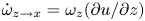 $\dot {\omega }_{z\rightarrow x}=\omega _z({\partial u}/{\partial z})$ and
  $\dot {\omega }_{z\rightarrow y}=\omega _z({\partial v}/{\partial z})$.
The following sections present a detailed description of the vorticity generation mechanisms of some of the most relevant features observed in §§ 5.1, 5.2 and 5.3. Section 5.5.1 focuses on the  $\omega _x$ generation that explains the alignment with
  $x$ of the initial hairpin vortex legs. Then, § 5.5.2 describes the
  $\omega _z$ generation mechanisms of the secondary roller vortex shown in figure 9. Lastly, § 5.5.3 addresses the early stages of the layered flow to understand the sources of
  $\omega _x$ that promote the streamwise alignment of vortical structures trapped between the liquid layers.
5.5.1. Stretching of the hairpin vortices
The initial velocity distribution described in § 2 results in a vortex sheet with only spanwise vorticity ( $\omega _z<0$), and a single non-zero velocity gradient (
 $\partial u/\partial y >0$). With the initial interface displacement, the major source of
  $\omega _x$ at the start of the simulation is the baroclinic term. After some time, vorticity is generated in the other directions and
  $\partial u/\partial x$ and
  $\partial u/\partial z$ are, in general, non-zero. Given the relative strength of
  $\omega _z$ and
  $\partial u/\partial y$ with respect to the other quantities,
  $\dot {\omega }_{y\rightarrow x}$ and
  $\dot {\omega }_{z\rightarrow x}$ become important
  $\omega _x$ generators. After the initial transient, Zandian et al. (Reference Zandian, Sirignano and Hussain2017, Reference Zandian, Sirignano and Hussain2018) show that, for low density ratios (i.e.
  $\rho _G/\rho _L$), the streamwise vorticity generation mechanism responsible for the formation of hairpin vortices in the gas phase is the baroclinic term. As the density ratio increases (i.e. the gas phase becomes denser), the relative importance of the baroclinic term diminishes due to its
  $\rho ^{-2}$ scaling in favour of
  $\dot {\omega }_{x\rightarrow x}$. In general,
  $\dot {\omega }_{z\rightarrow x}$ and
  $\dot {\omega }_{y\rightarrow x}$ are stronger than
  $\dot {\omega }_{x\rightarrow x}$, but they tend to cancel each other. A similar behaviour is observed in round jets (Jarrahbashi & Sirignano Reference Jarrahbashi and Sirignano2014).
This description explains the initial deformation of the KH roller vortex into a hairpin; thus, let us look at  $t^*>2$ to understand the additional stretching the vortex pins undergo. Zandian et al. (Reference Zandian, Sirignano and Hussain2017, Reference Zandian, Sirignano and Hussain2018) visualised the baroclinic term because their computations used a more diffuse interface capturing method (i.e. level-set). The density gradient between liquid and gas extends a few cells beyond the interface, allowing a smoother visualisation. However, our sharp interface VOF method concentrates the density gradient at the interface cells. Together with the pressure oscillations near the interface due to the generation of spurious currents, the baroclinic contribution of the two-phase flow cannot be properly visualised during the early times (see figure 19d). Once the mixing layers grow sufficiently, we can capture the baroclinic term.

Figure 19. Terms for generating  $\omega _x$ during the stretching of the initial hairpin vortex for case C1 at
  $t^*=3$: (a)
  $\omega _x$; (b) vortex stretching and tilting; (c) compressible stretching; and (d) baroclinic term. The front view from a
  $yz$ plane at
  $x=16\ \mathrm {\mu }\textrm {m}$ is shown. The interface is identified by the solid isocontour with
  $C=0.5$, and the cut vortex structures are identified by the dashed isocontour with
  $\lambda _{\rho,t}=-2.5\times 10^{15}$.
To understand the continuous stretching of the hairpin vortex pins, figure 19 shows the streamwise vorticity and its generation terms from (5.2) for case C1 at  $t^*=3$ in a
  $yz$ plane at
  $x=16\ \mathrm {\mu }\textrm {m}$. The
  $\omega _x$ contours in figure 19(a) resemble those in figure 6(f), which depicts
  $\omega _x$ at a later time. The vorticity vector is predominantly aligned with
  $x$ inside the vortex pins. Another region of strong
  $\omega _x$ appears between the hairpin and the liquid below. Despite the variable density in the transcritical flow, the vortex stretching and tilting terms are at least an order of magnitude larger than the compressible stretching or baroclinic terms. This characteristic repeats for all analysed cases. In our study, lower pressures are associated with larger characteristic velocities and milder density variations across the mixing regions. Thus, vortex stretching and tilting terms continue to dominate, even if the lower density in the gas phase favours a stronger baroclinic term.
The combined effect of vortex stretching and tilting increases the  $\omega _x$ magnitude in the vortex pins, effectively stretching the vortical structure. Compressible stretching opposes this deformation, but it has a weak contribution. Baroclinicity inside the vortex pins is not strong. Figure 20 presents the individual components of the vortex stretching and tilting terms from (5.2), and shows the partial cancellation of
  $\dot {\omega }_{y\rightarrow x}$ and
  $\dot {\omega }_{z\rightarrow x}$ reported in Zandian et al. (Reference Zandian, Sirignano and Hussain2017, Reference Zandian, Sirignano and Hussain2018). A closer look into figure 19(b) reveals that
  $\dot {\omega }_{x\rightarrow x}$ is relatively weak and does not justify the strong streamwise vorticity generation inside the vortex pins. Despite the partial cancellation,
  $\dot {\omega }_{y\rightarrow x}$ is larger than
  $\dot {\omega }_{z\rightarrow x}$ in some regions near the vortex pins, strengthening the combined effect of stretching and tilting. Although not presented here, a slice through
  $x=26\ \mathrm {\mu }\textrm {m}$ at
  $t^*=4.05$ shows that
  $\omega _x$ inside the vortex pins is still strong. Nonetheless, none of the terms of the streamwise vorticity equation significantly increase or decrease
  $\omega _x$ inside the vortex.

Figure 20. Terms for generating  $\omega _x$ during the stretching of the initial hairpin vortex for case C1 at
  $t^*=3$: (a)
  $\dot {\omega }_{x\rightarrow x}$; (b)
  $\dot {\omega }_{y\rightarrow x}$; and (c)
  $\dot {\omega }_{z\rightarrow x}$. The front view from a
  $yz$ plane at
  $x=16\ \mathrm {\mu }\textrm {m}$ is shown. The interface is identified by the solid isocontour with
  $C=0.5$, and the cut vortex structures are identified by the dashed isocontour with
  $\lambda _{\rho,t}=-2.5\times 10^{15}$.
All the terms in (5.2) contribute to increasing the magnitude of the  $\omega _x$ observed in figure 19(a) between the liquid surface and the hairpin vortex. Vortex stretching and tilting still dominate, but the contributions from volume dilatation and baroclinicity cannot be neglected. Figure 21 shows the gas-phase density, the pressure field relative to the ambient pressure and the divergence of the velocity field or volume dilatation rate. This snapshot's flow patterns reveal the vorticity generation mechanisms that occur throughout the computations in the variable-density transcritical flow. Note the local pressure minima inside the vortex pins in figure 21(b), which reflects the rationale behind the
  $\lambda _\rho$ vortex identification method. Moreover, the snapshot captures the interfacial pressure jump due to surface tension in the high curvature region near the lobe's tip.

Figure 21. Density in the gas phase, relative pressure,  $p_{rel}=p-p_{amb}$, and volume dilatation rate during the stretching of the initial hairpin vortex for case C1 at
  $t^*=3$: (a) gas density,
  $\rho$; (b) relative pressure,
  $p-p_{amb}$; and (c) volume dilatation rate,
  $\boldsymbol {\nabla }\boldsymbol {\cdot }\boldsymbol {u}$. The front view from a
  $yz$ plane at
  $x=16\ \mathrm {\mu }\textrm {m}$ is shown. The interface is identified by the solid isocontour with
  $C=0.5$ and the cut vortex structures are identified by the dashed isocontour with
  $\lambda _{\rho,t}=-2.5\times 10^{15}$.
The sign of the streamwise component of the baroclinic torque,  ${1}/{\rho ^2}(({\partial \rho }/{\partial y})({\partial p}/{\partial z}) - ({\partial \rho }/{\partial z})({\partial p}/{\partial y}))$, can be justified by looking at the density and pressure fields in figure 21. In general, the two-dimensional pressure gradient around the vortex pins (i.e. pressure gradient on the illustrated slice) is oriented radially outwards from each local pressure minimum. In contrast, the two-dimensional density gradient not only depends on the density jump across the interface, but also on the temperature and composition variations in the gas phase. Thus, the baroclinic term in (5.2) changes sign multiple times around the vortex pins, increasing and decreasing
  $\omega _x$ locally. For example, the sign of the baroclinic term in the region under the vortex pin centred around
  $z=22\ \mathrm {\mu }\textrm {m}$ in figure 19(d) is explained as follows. For
  $z<22\ \mathrm {\mu }\textrm {m}$, the baroclinic term is positive since
  ${\partial \rho }/{\partial y}<0$,
  ${\partial p}/{\partial z}<0$,
  ${\partial \rho }/{\partial z}>0$ and
  ${\partial p}/{\partial y}<0$. That is, both
  $({\partial \rho }/{\partial y})({\partial p}/{\partial z})>0$ and
  $-({\partial \rho }/{\partial z})({\partial p}/{\partial y})>0$ are positive and increase
  $\omega _x$ as depicted in figure 19(a). Then, the baroclinic term becomes negative for
  $z>22\ \mathrm {\mu }\textrm {m}$ because of the two-dimensional pressure gradient.
  ${\partial \rho }/{\partial y}<0$,
  ${\partial \rho }/{\partial z}>0$ and
  ${\partial p}/{\partial y}<0$ remain unchanged, but
  ${\partial p}/{\partial z}>0$. This change results in
  $({\partial \rho }/{\partial y})({\partial p}/{\partial z})<0$ and
  $-({\partial \rho }/{\partial z})({\partial p}/{\partial y})>0$, where the negative term dominates because the transverse density gradient and the spanwise pressure gradient are larger in magnitude than the spanwise density gradient and the transverse pressure gradient, respectively.
In contrast, the compressible vortex stretching sign is dictated by the local volume dilatation rate. If the fluid expands, the rotation of a fluid element is distributed over a larger volume, decreasing the vorticity magnitude. On the other hand, fluid compression increases vorticity. Here, the combination of the Stefan flow generated around the vaporising or condensing interface and the vortical flow determine the sign of  $\boldsymbol {\nabla }\boldsymbol {\cdot }\boldsymbol {u}$. Typically, the evaporation of the fuel results in a volume expansion near the interface. However, the transcritical environment introduces various changes in fluid behaviour. As discussed in § 5.1, the enhanced oxygen dissolution at 150 bar may result in net condensation. Therefore, volume compression occurs despite the evaporation of the fuel. In addition, density variations in the gas phase are more significant, and the increase in fuel vapour results in higher gas densities that could limit the expansive behaviour of evaporating flows.
Away from the recirculation region caused by the vortex pins, figure 21(c) reveals the local volume compression above the liquid surface, where weaker evaporation of the fuel results in net condensation. In contrast, the volume dilatation around the vortex structures behaves differently. On the one hand, the entrainment of the hot gas enhances the evaporation of the fuel, increasing the gas mixture density below the vortex pins. Thus, the lighter gas flows into a denser gas region, undergoing compression. On the other hand, the gas phase expands above the vortex pins. Fuel evaporation is stronger near the lobe's tip, substantially increasing the gas density in the surroundings. However, the vortical motion rapidly advects the gas into fluid regions of lower density.
The described  $\omega _x$ generation mechanisms for the stretching of the initial hairpin vortex do not change significantly across the analysed configurations that show lobe stretching, bending and perforation. Other deformation mechanisms show deviations in the evolution of the initial hairpin vortex. For example, figure 9 describing the lobe corrugation mechanism for case C2 shows a stronger stretching of the hairpin legs. Figure 22 depicts, for case C2, the streamwise vorticity and the combined contribution of vortex stretching and tilting in the generation of
  $\omega _x$. Two different
  $yz$ planes are shown: one at
  $x=12\ \mathrm {\mu }\textrm {m}$ and
  $t^*=2.5$ and the other at
  $x=28\ \mathrm {\mu }\textrm {m}$ at
  $t^*=4$. During the coupled deformation process between lobe and hairpin described in § 5.2,
  $\omega _x$ generation occurs inside the vortex pins, increasing the strength of each vortex. Here,
  $\dot {\omega }_{x\rightarrow x}$ is the main vorticity generation mechanism, having a similar magnitude as the vortex tilting terms that dominate in other flow regions. The behaviour of the compressible vortex stretching and the baroclinic terms is very similar to what has been described previously.

Figure 22. Terms for generating  $\omega _x$ during the stretching of the initial hairpin vortex for case C2: (a)
  $\omega _x$ at
  $x=12\ \mathrm {\mu }\textrm {m}$ and
  $t^*=2.5$; (b) vortex stretching and tilting at
  $x=12\ \mathrm {\mu }\textrm {m}$ and
  $t^*=2.5$; (c)
  $\omega _x$ at
  $x=28\ \mathrm {\mu }\textrm {m}$ and
  $t^*=4$; and (d) vortex stretching and tilting at
  $x=28\ \mathrm {\mu }\textrm {m}$ and
  $t^*=4$. The contours of the different terms are shown in
  $yz$ planes at various
  $x$ locations and times. The interface is identified by the solid isocontour with
  $C=0.5$, and the cut vortex structures are identified by the dashed isocontour with
  $\lambda _{\rho,t}=-9\times 10^{15}$.
The importance of the coupled deformation between the liquid surface and the hairpin vortex is revealed by comparing cases B1 and C2, both having a gas freestream velocity  $u_G=50\ \textrm {m}\ \textrm {s}^{-1}$. Case B1 shows a weaker contribution of
  $\dot {\omega }_{x\rightarrow x}$ in
  $\omega _x$ generation, and the hairpin deformation is consistent with the previous discussion of case C1. Not surprisingly, both cases B1 and C1 involve the same early deformation mechanism. Arguably, the term
  ${\partial u}/{\partial x}$ has a similar strength in cases B1 and C2. Thus, the amplified contribution of
  $\dot {\omega }_{x\rightarrow x}$ in case C2 must come from an
  $\omega _x$ increase in the vortex pins. As described in § 5.2, the lobe wraps around the vortex pins, enhancing the gas entrainment under the lobe as the gaps between the sides of the lobe and the liquid surface are reduced. This deformation process results in the strengthening of the
  $\omega _x$ (see figures 10 or 22).
5.5.2. The secondary roller vortex
New roller vortices form during the jet development, particularly in front of the main perturbation wave as it grows (see figure 13). These vortical structures are expected to emerge from the stretching of the vortex sheet between the liquid wave and the faster-moving gas. Along a sharp wave edge (i.e. a sharp flow turn), the vortex sheet separates and is rapidly affected by the gas entrainment underneath the liquid. Thence, a roller vortex forms. However, the formation of smaller roller vortices occurs without such a clear mechanism. For example, figure 9 shows that during the early lobe deformation in case C2, a small secondary roller vortex is observed on top of the hairpin vortex pins. No clear flow feature seems to explain its occurrence. Here, we describe the nature of the strengthening of the spanwise vorticity in that region, leading to the formation of the vortex.
The vortex formation mechanism originates in the destabilisation of the vortex sheet between liquid and gas. Figure 23 depicts the deformation of the early lobe as it corrugates between  $t^*=3$ and
  $t^*=4$, showing the vortex sheet (represented by the green isosurface with
  $\omega _z=-1.5\times 10^{7}\ \textrm {s}^{-1}$) and the hairpin vortex (red isosurface with
  $\lambda _{\rho,t}=-9\times 10^{15}$). The vortex sheet forms due to the shear between the two phases, and it follows the liquid surface along with the stretching and deformation of the lobe (i.e. the vortex sheet is also stretched and deformed). At
  $t^*=3$, no distinctive perturbation is seen. However, once the lobe bursts into small ligaments and droplets, the vortex sheet detaches from the liquid surface and is suddenly perturbed by the increased multiphase turbulence. This triggers a destabilisation of the vortex sheet and the formation of the secondary roller vortex, as explained in the following lines.

Figure 23. Destabilisation of the vortex sheet caused by the lobe bursting in case C2. The liquid surface is identified by the translucent blue isosurface with  $C=0.5$, the vortex structures are identified by the red isosurface with
  $\lambda _{\rho,t}=-9\times 10^{15}$ and the vortex sheet is identified by the translucent green isosurface with
  $\omega _z=-1.5\times 10^{7}\ \textrm {s}^{-1}$.
Figure 24 shows the evolution of the vortex sheet between  $t^*=4.25$ and
  $t^*=5$ after the lobe bursts. The contours of
  $\omega _z$ are shown in an
  $xy$ plane at
  $z=25\ \mathrm {\mu }\textrm {m}$, together with a three-dimensional view of the liquid surface and the vortex structures. To enhance the visualisation of the vortices in this figure,
  $\lambda _{\rho,t}=-5\times 10^{15}$ instead of
  $\lambda _{\rho,t}=-9\times 10^{15}$ used in previous figures for case C2 and the vortex isosurface is coloured with
  $\omega _z$. Pockets of stronger spanwise vorticity occur in the detached vortex sheet, as seen at
  $t^*=4.25$, arguably due to the interactions between ligaments and droplets. Over time, these vortical regions come together via mutual induction and subsequent pairing/merging, and some small roller vortices can be observed at
  $t^*=4.5$. In particular, one of these regions of vortex pairing grows considerably between
  $t^*=4.25$ and
  $t^*=5$, resulting in the formation of the secondary roller vortex seen in figure 9. Moreover, the strengthening of
  $\omega _z$ and the vortex pairing are aided by the induced flow coming from the hairpin vortex pins or legs. Once the lobe bursts, the vortex sheet is not only perturbed by the smaller liquid structures, but it is also under the direct influence of the hairpin vortex. Before, the presence of the liquid lobe between the vortex pins and the vortex sheet has a shielding effect.

Figure 24. Vortex pairing mechanism resulting in the formation of the secondary roller vortex in case C2. Contours of  $\omega _z$ are shown in an
  $xy$ plane at
  $z=25\ \mathrm {\mu }\textrm {m}$. The liquid surface is identified by the solid isocontour or the translucent blue isosurface with
  $C=0.5$, and the vortex structures are identified by the dashed isocontour or isosurface with
  $\lambda _{\rho,t}=-5\times 10^{15}$.
Figure 25(a) manifests the implications of this relative position between the vortex sheet and the hairpin vortex. The contours of  $\dot {\omega }_{z\rightarrow z}$ from (5.4) are shown in the same
  $xy$ plane from figure 24 at
  $t^*=4.25$. Due to the presence of
  $\omega _z$ and a spanwise stretching (i.e.
  $\partial w/\partial z>0$), there is
  $\omega _z$ generation that tends to strengthen the small vortices during the pairing process. Other terms in (5.4) have a negligible effect in the detached vortex sheet. As seen in figure 25(b), the hairpin legs (red vortex) are responsible for the spanwise stretching of the perturbed vortex sheet. Note that
  $\lambda _{\rho,t}=-5\times 10^{15}$ in this figure too. Moreover, the secondary roller vortex (green) wraps around the hairpin vortex pins, similar to how the liquid phase wraps around the vortical structures.

Figure 25. Spanwise vortex stretching affecting the formation of the secondary roller vortex in case C2: (a)  $\dot {\omega }_{z\rightarrow z}$ in the
  $xy$ plane at
  $z=25\ \mathrm {\mu }\textrm {m}$ and
  $t^*=4.25$; and (b) induced flow patterns from the hairpin vortex at
  $t^*=5$. The liquid surface is identified by the solid isocontour or the translucent blue isosurface with
  $C=0.5$, and the vortex structures are identified by the dashed isocontour or isosurface with
  $\lambda _{\rho,t}=-5\times 10^{15}$.
The mechanisms described in this section resemble the findings in previous works. The initial destabilisation or bursting of the vortex sheet is tightly coupled to the coiling of vortex lines and the turbulence cascade (Stout Reference Stout2021), here involving the multiphase flow. The later vortex pairing, emergence of the secondary roller vortex, and wrapping around the hairpin legs is a clear example of vortex reconnection (Hussain & Duraisamy Reference Hussain and Duraisamy2011; Stout & Hussain Reference Stout and Hussain2023; Yao & Hussain Reference Yao and Hussain2022).
5.5.3. Streamwise vortex alignment in the layered flow
Lastly, we look at the initial stages of the vortex alignment in the streamwise direction inside the layered flow. As seen in figure 14(c), which depicts a late snapshot of case C1 at  $t^*=15$ once various liquid layers have formed, some of the major structures contained in between the layers are aligned with
  $x$. In § 5.3, we describe how the vorticity within the layered flow primarily comes from the various roller vortices that form during the growth of the main perturbation wave. Other minor vortical structures also emerge in the layered flow, such as rim vortices or small roller vortices.
Figures 26 and 27 present the contour plots of different variables in a  $yz$ plane at
  $x=16\ \mathrm {\mu }\textrm {m}$ and
  $t^*=8.4$ for case C1. Figure 26 shows the various terms in (5.2), and figure 27 shows the vorticity components, the fuel vapour mass fraction, gas density and temperature. This non-dimensional time corresponds to the snapshot in figure 14(a), where the remnants of the roller vortex R2 are found underneath the liquid. At
  $x=16\ \mathrm {\mu }\textrm {m}$, the
  $yz$ plane cuts through the region where most of the vortex structures are. Despite being an early snapshot of the layered flow, the results in figure 26 provide relevant details of the
  $\omega _x$ generation mechanisms as the liquid layers form. Of course, other events impact the evolution of the vortical structures, such as the entrainment of the roller vortex R3, overlapping layers and frequent tearing and hole formation.

Figure 26. Terms for generating  $\omega _x$ in between the liquid layers for case C1 at
  $t^*=8.4$: (a) vortex stretching and tilting; (b)
  $\dot {\omega }_{x\rightarrow x}$; (c)
  $\dot {\omega }_{y\rightarrow x}$; (d)
  $\dot {\omega }_{z\rightarrow x}$; (e) compressible stretching; and (f) baroclinic term. The front view from a
  $yz$ plane at
  $x=16\ \mathrm {\mu }\textrm {m}$ is shown. The interface is identified by the solid isocontour with
  $C=0.5$ and the cut vortex structures are identified by the dashed isocontour with
  $\lambda _{\rho,t}=-2.5\times 10^{15}$.

Figure 27. Vorticity components, fuel vapour mass fraction, gas density and temperature in between the liquid layers for case C1 at  $t^*=8.4$: (a)
  $\omega _x$; (b) fuel vapour mass fraction,
  $Y_F$; (c)
  $\omega _y$; (d) gas density,
  $\rho$; (e)
  $\omega _z$; and (f) temperature,
  $T$. The front view from a
  $yz$ plane at
  $x=16\ \mathrm {\mu }\textrm {m}$ is shown. The interface is identified by the solid isocontour with
  $C=0.5$ and the cut vortex structures are identified by the dashed isocontour with
  $\lambda _{\rho,t}=-2.5\times 10^{15}$.
The contribution of vortex stretching and tilting to  $\omega _x$ generation mainly comes from
  $\dot {\omega }_{y\rightarrow x}$ and
  $\dot {\omega }_{z\rightarrow x}$. As reported in § 5.5.1, these two terms partially cancel each other. Note that
  $\dot {\omega }_{x\rightarrow x}$ has a weak contribution except in a region above the liquid core near the symmetry plane of the computations. Vorticity is predominantly aligned in the spanwise direction coming from the roller vortex R2, but streamwise vorticity is not negligible (see figure 27a,e). Thus,
  $\dot {\omega }_{x\rightarrow x}$ is not a major source of
  $\omega _x$, at least at this stage, because of a negligible
  $\partial u /\partial x$. In contrast to previous §§ 5.5.1 and 5.5.2, the contributions from variable-density effects become more important in the layered flow. Despite being an order of magnitude lower, compressible vortex stretching and baroclinicity affect flow regions where vortex stretching and tilting are weak. Therefore, these terms can be substantial drivers of
  $\omega _x$ and, in general, vorticity.
The increased importance of compressible terms is not unexpected. A closer look at the variations of composition, temperature and density in the gas phase is given in figures 27(b), 27(d) and 27(f). Multiple fuel-lean pockets are observed with higher temperatures and lower densities. These regions exist because of the entrainment of hotter ambient gas, as detailed in § 5.3 and visualised in figures 13–16. This increased complexity in the scalar mixing patterns results in a coupled mixing-deformation mechanism where vorticity defines the scalar mixing, which, in turn, affects vorticity generation and the vortex deformation due to the variable-density and compressible effects seen in (5.1). Scalar mixing patterns are also affected by vorticity at low ambient pressures. Nevertheless, the gas mixture density variations are often negligible at low pressures (Poblador-Ibanez & Sirignano Reference Poblador-Ibanez and Sirignano2018; Poblador-Ibanez et al. Reference Poblador-Ibanez, Davis and Sirignano2021), and a significant two-way coupling may not exist. Further analysis of this feature is beyond the scope of this work. Future studies of transcritical atomisation should address three key aspects together: (a) the liquid–gas mixing process (i.e. atomisation), (b) the mechanisms of scalar mixing (e.g. fuel mixing) and (c) the coupling with vorticity dynamics.
6. Summary and conclusions
The vortex dynamics analysis using the vortex identification method  $\lambda _\rho$ (Yao & Hussain Reference Yao and Hussain2018) reveals the interaction between deforming vortical structures and the liquid surface. It explains the deformation patterns identified in the temporal study of a transcritical planar liquid n-decane jet submerged into a faster and hotter gaseous oxygen stream presented by PS. Three main deformation mechanisms have been studied: the lobe stretching, bending and perforation mechanism, the lobe and crest corrugation mechanism and the layering of liquid sheets. The early lobe deformation is driven by the interaction between the liquid lobe and the initial roller vortex, which deforms into a hairpin. The heating of the liquid phase and the enhanced ambient gas dissolution at supercritical pressures generate significant variations of fluid properties across and along the interface. In particular, a liquid mixture with reduced density and gas-like viscosity is observed, and surface tension decreases rapidly. Thus, the vortical motion in the gas phase easily perturbs the liquid, which explains the lobe stretching, bending and corrugation mechanisms at relatively low velocities. During the growth of the primary perturbation, various strong roller vortices form and break up into smaller structures. These move underneath the wave at very high pressures (100 and 150 bar), triggering layering of the liquid into sheets. This process traps most of the vorticity generated during the early stages of liquid–gas mixing. It limits the formation of ligaments and droplets above the two-phase mixture, which tends to uniformise the flow (see PS). Nonetheless, the wave roll-up causes the entrainment of hotter liquid structures and hotter gas into a region of cooler temperatures, effectively mixing fluid regions with substantially different properties and generating fuel-rich or fuel-lean gas blobs. These gaseous regions of distinct fuel composition also exist outside the layered flow, resulting from the non-uniform fuel vaporisation and breakup of ligaments and droplets; thus, they might impact the combustion process. Their evolution is defined by the fluid dynamics and not only the high mass diffusivity characteristic of supercritical fluids.
Consistent with the literature, the alignment of vorticity with the streamwise direction explains the formation of three-dimensional perturbations responsible for atomisation. A look at the mechanisms for vorticity generation reveals that vortex stretching and tilting are the major contributors. Compressible vortex stretching and baroclinicity contribute to the vorticity generation everywhere in the mixing regions but are, in general, an order of magnitude lower. Moreover, variable-density and inertial terms induce different effects. Some regions show vortex stretching and tilting increasing vorticity, while compressible vortex stretching reduces it.
Regardless, variable-density terms become important in the layered flow due to the large differences in mixture composition, temperature and density. These observations highlight the strong two-way coupling between scalar mixing patterns and the development of vortical structures in the gaseous phase. Vorticity is responsible for the species and thermal mixing, modifying the mixture density and, in turn, the vorticity generation via compressible stretching and baroclinicity. This feature directly results from the transcritical environment since the variations in fluid properties are enhanced at high pressures. At low ambient pressures and similar low-Mach-number conditions, density changes in the gas phase are negligible despite the vaporisation of the fuel. Thus, only the scalar mixing is strongly affected by vorticity. Future studies of transcritical atomisation must address the liquid–gas mixing, the species and thermal mixing within each phase, and the coupling with vorticity dynamics to fully understand the physical mechanisms driving the liquid jet destabilisation and atomisation.
Acknowledgements
The authors are grateful for the support of the NSF grant with Award Number 1803833 and Dr R. Joslin as Scientific Officer. This work utilised the infrastructure for high-performance and high-throughput computing, research data storage and analysis, and scientific software tool integration built, operated and updated by the Research Cyberinfrastructure Center (RCIC) at the University of California, Irvine (UCI). The RCIC provides cluster-based systems, application software and scalable storage to directly support the UCI research community (https://rcic.uci.edu).
Funding
Additional computational resources included Stampede2 at the University of Texas at Austin, Bridges2 at the University of Pittsburgh and Expanse at the University of California San Diego, under the Extreme Science and Engineering Discovery Environment (XSEDE), which was supported by the NSF grant number ACI-1548562.
Declaration of interests
The authors report no conflict of interest.


 Open access