


1. Introduction
An example familiar to mariners is the tendency of a marine propeller operating under high loading conditions near the free surface to suddenly lose thrust when the propeller becomes aerated – a phenomenon known as ventilation. Ventilation is defined as the entrainment of incondensable gas into the liquid flow around a partially or fully submerged body. For ventilation to occur, the local fluid pressure must be less than the surrounding gas pressure, and there must be both a continuous source of gas (such as a free surface) and path between the gas source and low-pressure flow – conditions that have been established by Rothblum, Mayer & Wilburn (Reference Rothblum, Mayer and Wilburn1969), Swales et al. (Reference Swales, Wright, McGregor and Rothblum1974), Rothblum (Reference Rothblum1977) and that are summarized in Young et al. (Reference Young, Harwood, Montero, Ward and Ceccio2017).
Ventilation affects a wide range of lift-generating surfaces such as propellers, hydrofoils and control surfaces, and energy-saving or harvesting devices – especially highly loaded systems that operate at or near the free surface. Unanticipated atmospheric ventilation is particularly important to avoid, as it can cause drastic and sudden reductions in lift and thrust, which can lead to loss of vessel control, structural failure and potential for capsizing. While such multiphase flows can degrade hydrodynamic performance, they can also be used as an effective means of drag reduction or flow control through forced ventilation (pumping non-condensible gas to form a continuous gas bubble that envelops the majority of the body). Ventilation can also be used as an effective method of vibration reduction. As will be shown later in this paper, the amplitude of the load fluctuations can be reduced significantly by transitioning from fully wetted (FW) to a fully ventilated (FV) flow.
Although the last half-century has produced significant new knowledge on ventilation, previous studies focused mostly on the steady-state (SS) response of a rigid body. Recently, interest has grown in the transient motions of hydrofoils or vessels, waves, the unsteady flows produced by ventilation, the fluid–structure interaction (FSI) and the stability of ventilated surfaces. As most (linear elastic) materials deform in proportion to applied forces and inversely with the stiffness of the structure, highly loaded and high-aspect-ratio hydrofoils can sustain significant deflection. For example, if one were to observe composite hydrofoils in recent America's Cup competitions, foil deformations are often large enough to be observed with the naked eye. These deflections change the magnitude and orientation of the hydrodynamic load vector, as well as affect the structural dynamics of the foil and, hence, the vessel motions. Design solutions have been proposed that utilize the foil flexibility to delay or control natural ventilation (Young et al. Reference Young, Harwood, Montero, Ward and Ceccio2017). However, this requires an understanding of the nature of FSI in multiphase flow. Dynamic loading events caused by flow interactions with the lifting surface such as vaporous or gaseous cavity shedding, single-phase vortex shedding, wave-induced oscillations or maneuvers can produce significant vibratory responses in flexible hydrofoils (Harwood et al. Reference Harwood, Felli, Falchi, Ceccio and Young2019, Reference Harwood, Felli, Falchi, Garg, Ceccio and Young2020). The fluctuations in hydrodynamic loads from any such sources can be amplified if the frequency of oscillations drives resonance of or experiences locks-in with one of the system's natural frequencies, leading to reduced damping and dynamic load amplification. The resonant frequencies and damping of the hydrofoil can be strongly influenced by flow conditions such as submergence, speed, waves, cavitation and ventilation. If dynamic instability conditions such as flutter (when the net damping goes to zero for one of the modes) or parametric resonance (when the oscillation frequency is twice the fundamental natural frequency) are to be avoided, the changes in the system modal response with flow conditions must be understood. The changes in modal response due to flow conditions can also cause the reordering of structural modes due to changes in directionally dependent fluid inertia effects, which can lead to mode switching and frequency coalescence to cause dynamic instability (Harwood et al. Reference Harwood, Stankovich, Young and Ceccio2016b; Young et al. Reference Young, Wright, Yoon and Harwood2020). Additionally, ventilation can lead to large fluctuations in the fluid inertial, damping and restoring forces (Harwood et al. Reference Harwood, Felli, Falchi, Ceccio and Young2019, Reference Harwood, Felli, Falchi, Garg, Ceccio and Young2020), as well as significant dynamic load amplification due to lock-in resonance or parametric excitation (Akcabay & Young Reference Akcabay and Young2014; Smith et al. Reference Smith, Venning, Pearce, Young and Brandner2020a,Reference Smith, Venning, Pearce, Young and Brandnerb).
The focus of this work is on the influence of monochromatic non-breaking waves on the hydroelastic response of a surface-piercing hydrofoil in FW or ventilated flow. These foils operate at or near the free surface, thus, effects of waves must be considered as they can affect not only the dynamics of ventilation but the resulting forces and deformations. A related phenomenon to ventilation is cavitation, which involves a phase change between liquid and vapour, and will be discussed in Part 2.
1.1. Objectives
In this (Part 1) paper the focus is upon the sub-cavitating response of a flexible surface-piercing hydrofoil in waves. The objectives are to use experimental data to (1) explore how waves affect the quasi-steady and dynamic FW response; (2) explore how waves impact the inception and evolution of ventilation, as well as the resulting hysteresis and dynamic response; and (3) investigate how waves interact with vortex shedding, cavity shedding and structural dynamics. By addressing these points, the results of this work advance the collective knowledge of unsteady multiphase flows, multiphase FSI and the complex interactions between periodic flow features (waves, vortex shedding, cavity shedding) and the structural dynamics of flexible bodies.
2. Literature review
Here, we briefly review the hydrodynamics response in § 2.1 and hydroleastic response in § 2.2, followed by a review of the effect of waves on surface-piercing hydrofoils in § 2.3.
2.1. Hydrodynamic response of surface-piercing hydrofoils
The steady and unsteady characteristics of flow around surface-piercing hydrofoils has been summarized in depth by Breslin & Skalak (Reference Breslin and Skalak1959), Rothblum (Reference Rothblum1977), Harwood, Young & Ceccio (Reference Harwood, Young and Ceccio2016a) and Young et al. (Reference Young, Harwood, Montero, Ward and Ceccio2017). A brief summary follows, and readers are referred to those sources for additional details.
2.1.1. Flow regimes
The steady flow around a surface-piercing hydrofoil can be categorized as FW, partially ventilated (PV) or FV, distinguished by the extent and the stability of a ventilated gas cavity, as defined by Breslin & Skalak (Reference Breslin and Skalak1959), Harwood et al. (Reference Harwood, Young and Ceccio2016a) and Young et al. (Reference Young, Harwood, Montero, Ward and Ceccio2017).
2.1.2. Formation mechanisms of ventilation
The formation of a ventilated cavity can be deconstructed into two stages: inception and stabilization. Inception marks the transition from a FW flow to a PV flow, where the gas cavity begins to grow. Stabilization occurs as the cavity's size and the streamline kinematics reach a critical stability condition, at which point it is categorized as FV flow. Ventilation inception mechanisms rely both on the existence of a low-pressure region, as well as a path that can continuously entrain and transport gas to this region (Rothblum Reference Rothblum1977). The various mechanisms by which flow separation and/or air pathways produce ventilation formation have been extensively categorized (Swales et al. Reference Swales, Wright, McGregor and Rothblum1974; Young et al. Reference Young, Harwood, Montero, Ward and Ceccio2017), and a few dominant mechanisms are summarized below.
(a) Stall-induced ventilation occurs at high angles of attack as a result of massive flow separation from a foil's suction surface. Air is entrained either through the gradual depression of the free surface or through the low-energy pathways present in the vortical shear layer produced by stall.
(b) Tip-vortex-induced ventilation is a self-initiated mechanism for ventilation, caused by the aeration of a tip vortex. The large angular velocities of tip vortices cause low core pressures that will ingest air from the free surface at the distal end of the vortex. The persistence of tip vortices means that they may ingest air even very far downstream from the foil. When vortex core cavitation occurs, the vortex trajectory is pushed toward the free surface by buoyancy as well.
(c) Tail ventilation occurs when low pressures produce a strong downwards acceleration of the free surface. This in turn produces unstable growth of small perturbations (ripples, vortices, etc) that can draw air into ventilation-prone areas. These so-called Taylor instabilities (Taylor Reference Taylor1950) can be especially important when they occur on a thin sheet of liquid water separating the free surface from a vaporous cavity (Rothblum Reference Rothblum1977).
2.1.3. Elimination mechanisms of ventilation
The elimination of ventilated cavities encompasses the washout and rewetting events, respectively describing the transition from FV to PV and from PV to FW flows. Elimination tends to be driven by re-entrant jet instability at low speeds and moderate angles of attack (Harwood et al. Reference Harwood, Young and Ceccio2016a), turbulent reattachment at lower angles of attack and/or higher speeds (Young et al. Reference Young, Harwood, Montero, Ward and Ceccio2017) or cavity choking at high speeds, where a small airway feeding a larger submerged cavity collapses under the very low pressure produced by the constrained airflow (Wadlin Reference Wadlin1959; Elata Reference Elata1967).
2.1.4. Hysteresis response of ventilation
The hysteresis response of a surface-piercing foil is visible on both the lift and moment curves when plotted against the angle of attack curve or the Froude number. It has been shown that FV flow returns to the FW flow at a lower angle of attack and speed than the values at which ventilation was initiated, describing a hysteresis loop. The control of a ventilated foil is severely compromised as a result of this hysteresis, and the flow can assume several alternate, locally stable flow regimes (with widely varying hydrodynamic forces and moments) across a large range of speeds and angles of attack (Breslin & Skalak Reference Breslin and Skalak1959; Harwood et al. Reference Harwood, Young and Ceccio2016a). As a result, large changes in the attack angle, speed or both may be necessary to ensure that flow is unambiguously wetted or ventilated.
2.2. Hydroelastic response of surface-piercing hydrofoils
It is also important to consider how ventilation affects the structural response and dynamic stability of lifting surfaces, which are often relatively slender and compliant. The natural frequencies of a lifting body are largely dependent on flow conditions such as submergence, ventilation, cavitation and speed – especially for low-order (fundamental) modes (Fu & Price Reference Fu and Price1987; Kramer, Liu & Young Reference Kramer, Liu and Young2013; Motley, Kramer & Young Reference Motley, Kramer and Young2013; Young et al. Reference Young, Motley, Barber, Chae and Garg2016; Harwood et al. Reference Harwood, Felli, Falchi, Garg, Ceccio and Young2020). Immersion of a structure in a dense fluid produces inertial and damping effects in the fluid phase, termed fluid added mass and added damping. Hydrodynamic forces and moments that are proportional to structural displacements can be characterized as fluid disturbing forces (sometimes called hydrodynamic stiffness) (Harwood et al. Reference Harwood, Felli, Falchi, Ceccio and Young2019). Any phenomena that changes the hydrodynamic loading or the composition of fluid surrounding a flexible structure therefore produces an effect upon the fluid added mass, added damping and/or disturbing forces. Harwood et al. (Reference Harwood, Felli, Falchi, Garg, Ceccio and Young2020) showed experimentally that ventilation and cavitation caused a reduction in fluid added mass (attributed to the displacement of heavy fluid by light air). Effective mass and natural frequencies are also affected by partial submergence, which includes changes in draft or passage through waves (Fu & Price Reference Fu and Price1987; Kramer et al. Reference Kramer, Liu and Young2013; Motley et al. Reference Motley, Kramer and Young2013; Young et al. Reference Young, Motley, Barber, Chae and Garg2016; Harwood et al. Reference Harwood, Felli, Falchi, Garg, Ceccio and Young2020).
Changes in effective mass, damping and fluid disturbing forces can lead to linear resonance, parametric resonance, lock-in, modal coalescence and hydroelastic instabilities such as static divergence and flutter (Bisplinghoff, Ashley & Halfman Reference Bisplinghoff, Ashley and Halfman2013). Static divergence is a static instability that occurs when the fluid disturbing moment negates the structural elastic restoring moment, leading to unbounded growth in deformation until structural failure occurs. Flutter is a dynamic instability that occurs if the net fluid–structure damping of any mode reaches zero. Flutter is different from resonance, where external perturbations at one of the system natural frequencies are necessary. While single mode flutter has been observed (Besch & Liu Reference Besch and Liu1971; Brennen, Oey & Babcock Reference Brennen, Oey and Babcock1980), a coupled-mode flutter can also develop, where the modal frequencies of adjacent bending and torsional modes coalesce, and the damping of the torsional mode drops to zero (Akcabay & Young Reference Akcabay and Young2020). Flutter can develop as the changes in natural frequency and damping with flow conditions cause a reordering of the modes. Flutter instability of lightweight lifting bodies can occur at low frequencies, where a new bending-dominated mode is introduced by bend–twist coupling and the fluid disturbing force (Besch & Liu Reference Besch and Liu1971; Akcabay & Young Reference Akcabay and Young2020). The use of composites to build modern hydrofoils have made modal parameters more speed dependent due to their low solid-to-fluid density ratio (relative to metallic construction). As a result, the fluid component is made relatively more important and the response more sensitive to ventilation (Young et al. Reference Young, Wright, Yoon and Harwood2020).
Hydrofoils in operation are rarely subjected to only static loading conditions. Oscillatory loads such as waves, currents, vortex and cavity shedding and periodic forces produced by propellers or engines can excite various types of resonance of the fluid–structure system. The flow dependence of natural frequencies and damping ratios in compliant systems increases the risk of externally excited resonance. When an excitation is hydrodynamic in nature, lock-in can occur, which draws together nearby natural frequencies and the fluid excitations, leading to dynamic load amplification with reduced damping (Akcabay & Young Reference Akcabay and Young2015; Smith et al. Reference Smith, Venning, Pearce, Young and Brandner2020a). When flow conditions themselves are transient, the modulation of the fluid added mass and damping can produce parametric resonance (Akcabay & Young Reference Akcabay and Young2015). Flow-induced vibration affects ride quality and can result in unacceptable levels of noise and accelerated fatigue.
2.3. The effect of waves on surface-piercing foils
Surface waves on surface-piercing hydrofoils have been shown to significantly reduce the speed and angle of attack at which ventilation occurs. Originally investigated by McGregor et al. (Reference McGregor, Wright, Swales and Crapper1973), it was proposed that the steepness and accelerations of a surface wave are important characteristics that reduce the angle of attack at which struts ventilate. Experiments showed that the vertical acceleration of the wave and induced perturbations (such as waves breaking) are important factors that trigger early ventilation. A propagating wave induces wave orbital velocities and pressure gradients that affect Taylor instabilities and the strength of the surface seal. In addition to the effects of waves upon ventilation, their effects on the dynamic hydroelastic response of a hydrofoil is an important consideration (Young et al. Reference Young, Wright, Yoon and Harwood2020). Waves introduce oscillatory loads that vary with speed, relative wave direction and wave frequency. Similar to cavity shedding frequencies, waves can affect structural dynamics both as external excitation that can lock-in with the natural frequencies of the system and by modulating the fluid added mass, damping, or disturbing force in time. Young et al. (Reference Young, Wright, Yoon and Harwood2020) showed that non-breaking waves led to oscillatory hydrodynamic loads about mean values that matched those in calm water (CW). Additionally, changes to the structural dynamics were possible when the submerged aspect ratio varied, resulting in dynamic load amplification and significant flow-induced vibrations due to frequency coalescence caused by changes in the added mass at certain immersion depths (Young et al. Reference Young, Wright, Yoon and Harwood2020).
3. Prior experiments on a surface-piercing hydrofoil
Previous works that serve as the foundation for this study have been presented in (Harwood et al. Reference Harwood, Young and Ceccio2016a; Young et al. Reference Young, Garg, Brandner, Pearce, Butler, Clarke and Phillips2018; Harwood et al. Reference Harwood, Felli, Falchi, Ceccio and Young2019, Reference Harwood, Felli, Falchi, Garg, Ceccio and Young2020; Young et al. Reference Young, Wright, Yoon and Harwood2020). The present work builds upon these prior studies by using the same hydrofoil model and a similar instrumentation suite, so a brief review of those earlier experiments follows.
Previous tests were conducted in two different testing facilities: the Physical Model Basin (PMB) at the Aaron Friedman Marine Hydrodynamics Laboratory at the University of Michigan (UM) in Michigan, USA and at the free surface variable pressure recirculating water channel (also called the free surface cavitation channel) at the Italian National Research Council – Institute of Marine Engineering (CNR INM) in Rome, Italy. The PMB at UM has dimensions of 110 m long  $\times$ 6.7 m wide $\times$ 3.0 m deep and is equipped with a manned carriage and wave maker. The tank operates at atmospheric pressure, making it ideal for studying atmospheric ventilation, but not vaporous cavitation. Moreover, it is difficult to acquire sufficient data in a SS condition, as the SS time at the top speed of 6.2 m s $^{-1}$ is only two to three seconds. The free surface cavitation channel at CNR has a test section 10 m long $\times$ 3.6 m wide $\times$ 2.25 m deep. The recirculating channel has a top speed of 5.3 m s $^{-1}$ with a stable free surface. The cavitation channel can operate at pressures as low as 30 mbar allowing the channel to be used to study cavitation and ventilation. The theoretically unlimited time at steady state facilitates more extensive testing of FSI than is possible in a towing tank.
The focus of previous studies was to examine (1) ventilation formation and elimination mechanisms and boundaries in atmospheric and depressurized conditions in CW; (2) variation of SS hydrodynamic load coefficients with angle of attack ( $\alpha$), submerged aspect ratio ( $AR_h=h/c$, with $h$ and $c$ as the foil submergence depth and chord, respectively), submerged-depth based Froude number ( $F_{nh} = U/\sqrt {gh}$, with $U$ as the SS speed) and free surface cavitation number ( $\sigma _v={(P_t-P_v)}/{(0.5\rho U^2)}$, with $P_t$ and $P_v$ as the tunnel and vapour pressure, respectively); (3) influence of foil flexibility on the hydrodynamic load coefficients and ventilation boundaries; (4) variation of the generalized fluid (added mass, damping and disturbing) forces with operating conditions, and resulting change on the system resonance frequencies and damping coefficients; and (5) influence of waves on the SS and dynamic performance of the surface-piercing hydrofoil in an atmospheric towing tank. It should be noted that, although the influence of waves was presented in Young et al. (Reference Young, Wright, Yoon and Harwood2020), experimental data are limited to short-duration SS tests at atmospheric pressure.
3.1. Foil geometry and structural properties
All of the prior and present work used a canonical rectangular surface-piecing strut/hydrofoil with a nominal chord of  $c=27.9$ cm, a trailing edge thickness of $\tau =2.79$ cm and a span of $S=91.4$ cm. The cross-section has a circular-arc forebody with a radius of curvature of 84.8 cm and a rectangular afterbody. Three variants of this design were tested: a stiff (practically rigid) aluminium hydrofoil (model 0, made of 6061 aluminium), a flexible PVC hydrofoil (model 1) and a reinforced PVC hydrofoil (model 2). Model 0 and model 1 share identical geometry. Model 2 is simply model 1 reinforced with a 6.35 mm thick aluminium strip attached to the foil trailing edge (TE), as shown in figure 1.
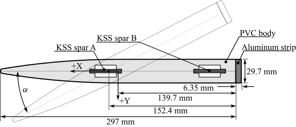
Figure 1. A section view of the geometry of the reinforced PVC (model 2) surface-piercing strut with rectangular planform as shown in figure 2. Model 0 and model 1 have the same geometry but do not have the aluminium strip at the foil TE. All dimensions are in millimetres.
Table 1 lists the structural properties of the three hydrofoil variants. As shown in the data in Ward, Harwood & Young (Reference Ward, Harwood and Young2018), Harwood et al. (Reference Harwood, Young and Ceccio2016a, Reference Harwood, Felli, Falchi, Ceccio and Young2019), the aluminium hydrofoil (model 0) was rigid enough that FSI effects were negligible. The flexible PVC hydrofoil (model 1) underwent noticeable deformation (maximum tip bending to chord ratio of  $\delta /c = 0.18$ and maximum tip twist of $\theta = 4^\circ$ under the maximum loading condition of 200 N), so FSI effects were significant. Compared with model 1, the reinforced PVC hydrofoil (model 2) has a much higher flexural rigidity (increased by 62.5 %), torsional rigidity (increased by 74 %) and its elastic axis ( $X_{sc}/c$) is shifted aft, as shown in table 1. Note that model 2 was used exclusively in the present work, as it elicited significant FSI response without the excessive bending deformations of model 1.
Table 1. Physical properties of the three surface-piercing struts and the specific test facility in which each was tested. Note that model 2 is used exclusively in this work. Model 0 and model 1 data are provided for completeness.

3.2. Previous experimental set-up
In all tests, the hydrofoil was clamped at the root and mounted to a load cell measuring forces and moments in all six degrees of freedom (ATI Omega-190), as shown in figure 2. The measurement uncertainty of the load cell is estimated to be  $\pm$2.6 % of the mean values. In all the work presented, the measurements are reported about the mid-chord at the root of the foil, as illustrated in the coordinate system shown in figures 1 and 2.

Figure 2. Rendering of the surface-piercing strut and experimental apparatus. Figure reproduced from Harwood et al. (Reference Harwood, Felli, Falchi, Ceccio and Young2019).
Inside the hydrofoil there are two instrumented aluminium kinematic shape sensing (KSS) spars embedded into milled slots, which are spaced 12.3 cm apart along the chord, as shown in figures 1 and 2. In the tests conducted at UM and CNR, the spars were designed to measure bending and torsional deformations, from which time- and frequency-domain analysis of foil deformations were carried out, including the direct extraction of structural mode shapes. Details may be found in Di Napoli et al. (Reference Di Napoli, Young, Ceccio and Harwood2019) and Harwood et al. (Reference Harwood, Felli, Falchi, Ceccio and Young2019).
3.3. Foil modal characteristics
Harwood et al. (Reference Harwood, Felli, Falchi, Garg, Ceccio and Young2020) used input–output analysis to extract modal parameters from the model 2 hydrofoil at varying immersion depths. The measured modal frequencies plotted against the submerged aspect ratio ( $AR_h=h/c$) in figure 3. The small, filled symbols and larger open symbols show data from UM and CNR, respectively. Young et al. (Reference Young, Wright, Yoon and Harwood2020) used a curve fit of the measured added-mass coefficients of Harwood et al. (Reference Harwood, Felli, Falchi, Garg, Ceccio and Young2020) to model the effect of partial immersion on natural frequencies, the results of which are denoted as ‘pre’ for both FW and FV flows. Mode 1 is the first bending mode, mode 2 is the first twisting mode, mode 3 is the second bending mode, mode 4 is the lead-lag mode and mode 5 is the third bending mode (Harwood et al. Reference Harwood, Felli, Falchi, Garg, Ceccio and Young2020). Figure 3 indicates that all of the modal frequencies except for the pure lead-lag or surge mode ( $\,f_4$) decrease with increasing immersion. This decrease occurs as a result of added mass, which increases as the projected area of the submerged portion of the hydrofoil increases. The lead-lag mode (mode 4) could not be measured using the KSS spars, but a numerically predicted dry resonance of $\,f_4 = 64.4$ Hz was obtained from a finite element model (FEM). The lead-lag mode possesses a negligibly small swept volume, in theory, has near zero added mass for a very thin body at zero angle of attack. Good agreement is observed between data collected from UM and CNR and the data also agrees well with the predicted values.

Figure 3. Experimental and predicted modal frequencies (modes 1–5) in dry and wetted conditions across a range of submerged aspect ratios ( $AR_h=0\unicode{x2013}2.5$). Results are shown for the reinforced PVC hydrofoil (model 2) from testing at UM and CNR. Symbols denote experimental values. Dashed lines indicate values for FW and FV flows made using a semi-empirical model. As the submergence increases, the natural frequencies (except for mode 4, the lead-lag mode) decrease. Note that modes 2 and 3 coalesce between $AR_h=2.0$ and $2.5$.
In all cases except for mode 4, FV frequencies are higher than their FW counterparts, driven by a decrease in added mass as the water on the suction side is replaced with gas (Harwood et al. Reference Harwood, Felli, Falchi, Garg, Ceccio and Young2020), with the magnitude of the change dependent upon both  $AR_h$ and the mode shape. In general, for a streamlined lifting surface with $AR_h > 1$ and cantilevered at the root, the added-mass effect is greater for bending-dominated modes than for twisting-dominated modes. As a result, bending and twisting modes with only a moderate frequency separation in air can overlap with one another as $AR_h$ changes – a process known as frequency coalescence. As shown in figure 3, coalescence between modes 2 and 3 occurs at $AR_h \approx 2.0\unicode{x2013}2.5$, which will lead to dynamic load amplification.
4. Experimental set-up at MARIN depressurized wave basin
To examine the interaction of waves with a surface-piercing foil undergoing cavitation and ventilation, tests were conducted at the Depressurized Wave Basin (DWB) at MARIN. The DWB is 240 m long  $\times$ 18 m wide $\times$ 8 m deep. The unmanned towing carriage can achieve a maximum SS speed of 6.0 m s $^{-1}$ measured with an uncertainty of 0.061 %. The facility can generate waves with a maximum wave height of 0.4 m and a period of 3 s. The pressure of the DWB can be reduced to 29 mbar and was measured using a Rosemount 3051 pressure transmitter, with a measurement range of 4–800 mbar and an uncertainty of 0.02 %. The tests were conducted at the end of January 2020, at which time the water temperature in the tank was approximately 12 $^\circ$C, measured using a TR25 modular RTD thermometer. The density, viscosity and vapour pressure of water is computed based on the instantaneous measured temperature using water properties according to IAPWS IF-97. A schematic of the test set-up is shown in figure 4. Two high-speed underwater cameras were placed to observed the submerged portion of the hydrofoil – both set to acquire monochrome images at 500 Hz. A photron multi camera was placed on the suction side of the hydrofoil foil to observe the ventilation patterns and an IDT Os7 camera was placed aft of the hydrofoil to observe the TE deflection patterns. Bradley BE HD10 cameras were used to acquire colour video above the waterline at 25 Hz. Forces and moments were measured using the same six degrees of freedom load cell used in previous experiments. Deflections were measured using redesigned KSS spars inserted into the slots of the hydrofoil. In the present work only the aft KSS spar was used, which included four full-bridge strain gauges – four bending type and four shear type. Wave elevations were measured using a capacitance wave height transducer placed at a lateral distance of 1.97 m (measured from the centre of the load cell). The data acquisition system was an HBM Quantum, with MX840B and MX411 modules and operated with Marin measurement system software. The sampling frequency was set to $F_s=4800$ Hz and the videos were correlated in time with the measurements of the forces and deformations.

Figure 4. Schematic overview of the basin and the location of the test set-up (including start and stop position adopted for the measurements).
The DWB allowed for properly scaled hydrodynamics of cavitation and ventilation by varying the tunnel pressure, carriage speed, foil submergence, wave height and wave period. The physical dimensions allow for a sufficient time at constant velocity for dynamic measurements with negligible side-wall or bottom interactions. Tests were divided into two days, with day one dedicated to atmospheric pressure and day two dedicated to reduced pressure/cavitation.
4.1. Summary of test condition at the DWB at MARIN:  $P_t=P_{atm}$

The range of test parameters in atmospheric conditions ( $P_t=P_{atm}$) at the DWB at MARIN are summarized in table 2. The flow conditions are characterized by the immersed aspect ratio ( $AR_h=h/c$), angle of attack ( $\alpha$), depth-based Froude number ( $F_{nh}=U/\sqrt {gh}$, where $U$ is the SS speed and $g$ is gravitational acceleration), incident wave period ( $T_w=1/f_w$) and incident wave amplitude ( $A_w$). The non-dimensional wavelength to immersion depth ratio ( $\lambda _w/h$), and incident wave amplitude to wavelength ratio ( $A_w/\lambda _w$), as well as wavelength to chord length ratio ( $\lambda _w/c$) are also reported.
Table 2. Test matrix of the experiments conducted at the DWB at MARIN under atmospheric test conditions on day 1 ( $P_t=P_{atm}=101.3$ kPa).

4.2. Test and analysis procedure
Each trial was started with the carriage at rest. The carriage was then accelerated to its target SS speed, which was maintained for a pre-determined period of time before decelerating. The towing tank was permitted to settle for 20–30 minutes between tests. The influence of acceleration and deceleration rates were examined between the allowed range of 0.1–0.45 m s $^{-2}$. Ventilation inception was observed earlier (at lower speeds) for cases with acceleration rates below 0.3 m s $^{-2}$. Faster acceleration delayed ventilation inception because the acceleration reduces the instantaneous adversity of the pressure gradient on the suction side Harwood et al. (Reference Harwood, Young and Ceccio2016a). The effects of different deceleration rates were observed to be negligible on the mean and dynamic response for cases with the same flow regime.
Bias measurements were acquired at zero speed at both the start and end of each trial, allowing corrections to be made for short-term drift in signals. For measurements with waves, calibrated regular waves were generated from the wave generators placed at the end of the basin (see figure 4). The carriage was held stationary until the generated wave train reached the opposite side of the basin (start position) to avoid wave reflection effects. As the wave characteristics were well within the basin's operational profile, no significant energy dissipation was expected or observed.
To separate the slowly moving mean from the dynamic fluctuations of the hydrodynamic load coefficients and tip deformations, the ‘movmean’ algorithm in Matlab was used to find the moving mean, which was then subtracted from the raw signal to obtain dynamic fluctuations. The width of the moving mean window was 1 s of data for cases without waves and four wave encounter periods (4 $T_e$) for cases with waves. The wave encounter period is defined using the SS speed $U$, where $T_e=1/f_e$. Here $\,f_e$ is the wave encounter frequency,
 \begin{equation} f_e=\frac{1}{2 \pi}\left\{\omega_w+\frac{\omega_w^2U}{g}\right\}, \end{equation}
with  $\omega _w=2\pi /T_w$.
The ‘pwelch’ algorithm in Matlab was used to estimate the power spectral density (PSD), where the number of FFT points was selected to yield a minimum frequency resolution of 0.5 Hz and the minimum window length was set to 2 s. Comparison of PSDs obtained over the full test duration for each run with that obtained over the steady-speed region only showed a negligible difference, and, hence, the PSDs shown in the subsequent section are obtained using the full test duration, from the start to the stop of the carriage, for each run. To illustrate transient events (such as sudden transition from FW to FV flows), the time-frequency spectra are obtained using the wavelet synchrosqueezed transform (WSST) via Matlab, which is based on the work of Thakur et al. (Reference Thakur, Brevdo, Fučkar and Wu2013). The WSST is used instead of the continuous wavelet transform to minimize energy smearing. The time-frequency spectra are also useful in depicting the change in vortex shedding frequencies ( $\,f_{vs}$) during the acceleration and deceleration stages, and the effect of wave-induced modulations on the modal frequencies and vortex shedding frequency. Based on past experimental data presented in Harwood et al. (Reference Harwood, Young and Ceccio2016a, Reference Harwood, Felli, Falchi, Ceccio and Young2019, Reference Harwood, Felli, Falchi, Garg, Ceccio and Young2020) and Young et al. (Reference Young, Wright, Yoon and Harwood2020) vortex shedding from the foil TE occurs at a constant Strouhal number ( $St$) based on the foil TE thickness ( $\tau$),
 \begin{equation} St=\frac{f_{vs}\tau }{U}=0.265. \end{equation}
 While the PSD and time-frequency spectra of the measurements can be used to identify the frequency peaks, it is important to relate the peaks to the various sources of excitation. The foil modal frequencies are known from prior tests (figure 3). Here  $\,f_e$ and $\,f_{vs}$ are computed using (4.1) and (4.2), respectively. The carriage modal frequencies were measured using a three-axis accelerometer (PM Instrumentation OS-315LN) attached to the carriage. The measurements were conducted by running the carriage without the foil and the mounting set-up at varying speeds. The dominant carriage modal frequency in the axial ( $x$) direction was found to be 18 Hz and the lateral ( $y$) direction was found to be 1.2 Hz. The lateral carriage frequency of 1.2 Hz is lower than the fundamental foil modal frequency and the lowest expected wave encountered frequency at 1.37 Hz for $F_{nh}=1.5$, $AR_h=1$ and $T_w=1.5$ s. Hence, lateral carriage mode is not included in the results. retain your intended meaning or clarify. The axial carriage modal frequency is marked as $\,f_{car}=18$ Hz in the plots depicting the frequency and time-frequency spectra.
4.3. Stochastic subspace identification-spectral proper orthogonal decomposition co-analysis
In addition to providing time-resolved measurements of flexural and torsional displacements, the KSS spars were used to assess the effects of flow regime upon dynamical system properties. Unlike the input–output analyses adopted by Phillips et al. (Reference Phillips, Cairns, Davis, Norman, Brandner, Pearce and Young2017) and Harwood et al. (Reference Harwood, Felli, Falchi, Garg, Ceccio and Young2020), the emphasis in this work was placed upon output-only analysis, wherein the excitation is assumed to be provided by the ambient flow and remains unobserved. The output-only system identification and its pairing with complementary videographic analysis were adopted from Di Napoli (Reference Di Napoli2022) and are summarized in the following subsections.
4.3.1. Output-only modal analysis
Parameter estimation was used to extract significant operational modal properties from the output data. This class of data analysis is often referred to as output-only or operational modal analysis. These methods were developed for the study of structural modes and responses when there is no input available, and it is used here for the analysis of the operational modal characteristics across a range of flow conditions. The covariance-driven stochastic subspace identification (SSI-COV) algorithm (Aoki Reference Aoki1987; Peeters & De Roeck Reference Peeters and De Roeck1999) was used for computational efficiency. The flow chart of the SSI-COV algorithm used to compute the modal eigenfrequencies (modes) and mode shape is shown in figure 36. A more detailed description of the algorithmic procedure is given in § A.1 in the Appendix A. As with any output-only method, a few caveats apply. The modes from an output-only analysis should be treated carefully. Peaks in the excitation spectra – such as those caused by periodic hydrodynamic phenomena – will cause forced-vibration responses that may be interpreted as structural resonance. Stochastic subspace identification also produces complex-valued modes, wherein node lines change in time. In this work, each complex mode shape was rotated to maximize the Euclidean norm of its real part, which was shown by Ahmadian, Gladwell & Ismail (Reference Ahmadian, Gladwell and Ismail1995) to maximize the similarity between a complex mode and its associated (real) normal mode shape. The real part was then used for plotting, discarding phase information. The complex modes can be viewed as animated movies in the online supplementary materials available at http://doi.org/10.1017/jfm.2023.127. The associated mode shapes should also be more correctly referred to as operating deflection shapes (ODS). In the following results and discussion, the term mode shape will be used in association with a structural resonance, while ODS will be used to describe the shape of the forced-vibration response of the hydrofoil. Finally, the damping estimates from SSI are also influenced by the shape of the input spectrum, so the reported damping ratios should be interpreted qualitatively, rather than quantitatively.
4.3.2. Spectral proper orthogonal decomposition of video
Spectral proper orthogonal decomposition (SPOD) was used to identify energy ranked and spatio-temporally orthogonal modes (Schmidt et al. Reference Schmidt, Towne, Rigas, Colonius and Bres2018; Towne, Schmidt & Colonius Reference Towne, Schmidt and Colonius2018a) from high-speed video records for each run. Smith et al. (Reference Smith, Venning, Pearce, Young and Brandner2020a,Reference Smith, Venning, Pearce, Young and Brandnerb) used SPOD to excellent effect to explore the patterning of cavitation shedding on a flexible hydrofoil. In this work, SPOD was performed on the video recordings from the underwater high-speed camera imaging the foil's suction surface, with durations ranging from 25 to 45 s. Each video was cropped to a region of interest containing the suction side of the hydrofoil, the free surface and the visible portion of the wake. The MATLAB SPOD toolbox published by Towne et al. (Reference Towne, Schmidt and Colonius2018a), Schmidt et al. (Reference Schmidt, Towne, Rigas, Colonius and Bres2018) was used for the decomposition. To further economize calculations, frames were downsampled to a rate of 166.67 Hz. Windowing was specified with 2048 frames with a 75 % overlap, and only the single most energetic mode at each frequency was selected for plotting in the results to follow.
4.3.3. Co-analysis procedure
A co-analysis framework proposed by Di Napoli (Reference Di Napoli2022) was used to illustrate the interactions between ambient hydrodynamic modes and structural modes. The co-analysis workflow is depicted in figure 5. For a given run, the SPOD spectrum was pre-computed for the selected region of interest of the video. Stochastic subspace identification was then performed on a subset of ten bending, ten torsion and single yawing-moment time series, with a model order interactively specified by the user, producing a set of candidate poles representing both resonant modes and flow-induced vibration. The SPOD videographic modes were then extracted at only those frequencies most closely matching the imaginary component of each pole fitted by SSI. These videographic modes indicate the presence of any spatially coherent flow patterns that may be associated with – and occurring at the same frequency as – the structural vibration, thus disambiguating the candidate pole as a system resonance, a forced vibration or a spurious artifact. In the following results, distinctions will be made between the hydrodynamic modes and the structural modes or ODS. Additional details about the SPOD analysis can be found in § A.1.4 in the Appendix A.

Figure 5. Workflow for SSI-SPOD co-analysis. Here SSI is used to estimate system poles from SS bending and twisting measurements. Those poles are used to specify the frequencies at which synchronous videographic SPOD modes are extracted. Both resonant and forced-vibration responses are thus analysed in both solid and fluid domains, allowing the causality of the hydro-structural responses to be explored.
5. Steady-state hydrodynamic response
Figure 6 illustrates the influence of  $F_{nh}$, $AR_h$ and $\alpha$ on the mean lift ( $C_L$), moment ( $C_M$) and drag ( $C_D$) coefficients at atmospheric pressure. The coefficients are defined as
 \begin{equation} \left.\begin{aligned} C_L=\frac{L}{\rho U^2 A/2}, \\ C_D=\frac{D}{\rho U^2 A/2}, \\ C_M=\frac{M}{\rho U^2 A c/2}, \end{aligned}\right\} \end{equation}
where  $L$,
$L$,  $M$ and $D$ are the lift, moment and drag values, $\rho$ is the fluid density, $U$ is the SS speed and $A=ch$ is the submerged projected area with $c$ as the nominal chord and $h$ as the foil submergence depth. All load coefficients shown in this work are defined about the mid-chord at the root (fixed end) of the hydrofoil and are non-dimensionalized using the average of the measured speed in the steady-speed region, $U$. To illustrate the repeatability of the results across different facilities experimental data collected at atmospheric pressure across all three facilities (UM, CNR and MARIN) are shown, illustrating excellent cross-facility repeatability.

Figure 6. Influence of  $F_{nh}$ and $AR_h$ on the mean FW and FV load coefficients defined about the mid-chord. Open and filled symbols indicate FW and FV measurements, respectively. The blue and red results correspond to $F_{nh}$ of 1.5 and 3.0, respectively. The circle and square symbols correspond to measurements from UM and CNR, while the diamonds and stars correspond to measurements from MARIN, including both CW and wave runs. The measurements from all three facilities agree well with one another and with semi-empirical predictions (shown as blue lines for $F_{nh} = 1.5$ and red lines for $F_{nh} = 3.0$). The results show the hysteresis and bi-stable response between the FW (top curve) and FV (bottom curve) flow in each plot. The results also show the hydrodynamic load coefficients and the flow transition boundary in atmospheric conditions depends on the angle of attack ( $\alpha$), submerged aspect ratio ( $AR_{h}$) and Froude number ( $F_{nh}$). The drop in the load coefficients due to transition from FW to FV flow is more severe for cases with higher $F_{nh}$, and occurs earlier for cases with higher $AR_h$ and higher $F_{nh}$ because of higher lift and lower pressures.
The MARIN data includes the mean values from both CW and wave runs, obtained by averaging the measured values in the steady-speed region for each run. In some cases, the flow changed from FW to FV during the steady-speed region. In those cases, the average of the measured values in the FV portion of the steady-speed region was used. The MARIN data (represented by diamonds for  $F_{nh} = 1.5$ and stars for $F_{nh} = 3.0$) agrees well with data from UM and CNR (represented by circles for $F_{nh} = 1.5$ and squares for $F_{nh} = 3.0$). Open and filled symbols represent FW and FV measurements, respectively. The predictions shown by the blue dashed and blue dashed-dotted lines for $F_{nh} = 1.5$, and red dotted and red solid lines for $F_{nh} = 3.0$ are based on modified semi-empirical predictions from Damley-Strnad, Harwood & Young (Reference Damley-Strnad, Harwood and Young2019). The focus of this paper is on the experimental analysis, and the predictions are only provided to help clarify trends due to the limited number trials possible with facility time and cost limitations.
Figure 6 shows that in the FW flow, the top curves in each subplot, the load coefficients initially increase as the angle of attack ( $\alpha$) increases, then decrease sharply (in the form of a vertical drop) when the flow transitions from FW to FV flow. Once the flow is FV, further changes in $\alpha$ cause $C_L$ to move along the bottom FV curve. The flow re-wets when the FV curve meets the FW curve, forming a hysteresis loop. While $C_L$ remains fairly linear with variations in $\alpha$ in the FW regime, $C_M$ becomes nonlinear prior to the transition to FV flow due to the shifting of the centre of pressure towards the mid-chord when the suction surface is enveloped in a cavity at constant pressure. A more severe drop is also observed in $C_M$ compared with $C_L$ when the flow transitions from FW to FV flow. The FV values of $C_D$ can be higher or lower than the FW $C_D$ due to competing changes such as reductions in lift-induced and frictional drag, and increases in form and spray drag in the FV flow.
As  $F_{nh}$ increases, ventilation incepts earlier, as indicated by the earlier (lower $\alpha$) drop in load coefficients for the red curve at $F_{nh}=3.0$ compared with the blue curves at ${F_{nh}=1.5}$. The FW load coefficients in figure 6 have minimal dependence on $F_{nh}$. The FV lift and moment coefficients decrease with higher $F_{nh}$ because of a lower effective camber caused by the concave shape of the pressure-side streamline surrounding the foil and the ventilated cavity. As a result, the reduction in load coefficients from FW to FV flow is more pronounced for cases with higher $F_{nh}$.
Comparison of the top and bottom row of results in figure 6 shows that the load coefficients increase with higher  $AR_h$ due to reduced three-dimensional (3-D) effects and losses at the free surface and tip, as well as losses caused by spanwise flow and jet sprays. The transition from FW to FV flow occurs at a slightly lower $\alpha$ with higher $AR_h$ and higher $F_{nh}$ due to higher suction/lift, which increases the downward depression of the free surface and accelerates ventilation. The mean load coefficients from the CW and wave runs from MARIN are plotted using the same symbols and colours, as there is no distinguishable difference between them as long as the flow regime remains the same. However, as will be shown in the next section, waves affect the flow transition boundary, as well as the dynamic response of the hydrofoil.
6. Dynamic hydroelastic response
The focus of this section is on the effect of waves, attack angle, speed and partial immersion on the dynamic hydroelastic response of the hydrofoil in FW and ventilated flows, presented in five subsections. The influence of  $\alpha$ and waves at $AR_h = 1$, $F_{nh} = 1.5$ is presented in § 6.1, and at $AR_h = 2$, $F_{nh} = 1.5$ in § 6.2. A comparison of the results in these two subsections showcases the effect of $AR_h$. To illustrate the influence of $F_{nh}$ and waves, results for $\alpha = 5^\circ$, $AR_h = 1$ are shown in § 6.3. Near the ventilation transition boundary, the flow is highly sensitive to random variations in the flow, and the effect is illustrated in § 6.4 for cases in CW and in § 6.5 for cases in waves. In all the plots shown in this section, $iFV = 0$ and $iFV=1$ refer to FW and FV flows, respectively, and $iwave = 0$ and $1$ refer to CW and wave runs, respectively. Here $\sigma _v = {(P_{t} - P_v)}/{(0.5\rho U^2)}$ is the vapour-pressure-based cavitation number defined at the free surface.
6.1. Influence of $\alpha$ and waves: $AR_h = 1, F_{nh} = 1.5$


To examine the influence of  $\alpha$ and waves at $AR_h = 1$, $F_{nh} = 1.5$, results for $\alpha = 5^\circ$ and $\alpha = 15^\circ$ are presented in §§ 6.1.1 and 6.1.2, respectively. The influence of varying $\alpha$ compiled together are presented in §§ 6.1.3.
6.1.1. $\alpha = 5^\circ, AR_h = 1, F_{nh} = 1.5$

Figure 7 shows photos (taken from above and below the water surface) of two FW runs: run 1001 in CW in (a) and run 1601 in waves in (b). Both runs are identical except for the presence of regular waves (with wave amplitude  $A_w$ of 0.05 m and wave period $T_w$ of 1.5 s) in run 1601. The corresponding time histories of the hydrodynamic load coefficients and tip deformations for both runs are compared in figure 8. Figure 9 compares the PSDs of the fluctuating hydrodynamic load coefficients and tip deformations.

Figure 7. Above water view (top) and underwater view (bottom) of the suction side of the foil for a CW run (a) and a run in waves with  $T_w=1.5$ s, $A_w=0.05$ m (b) at $\alpha = 5^\circ$, $AR_h=1$, $F_n=1.5$, $P = P_{atm}$. Two snapshots are shown for the run in waves, the first showing a wave trough and the second a wave crest at the location of the foil's leading edge. Both runs are FW. The free surface is depressed near the foil TE due to the suction created by the foil. An aerated triangular base cavity forms in the separated flow behind the TE, the length of which decreases with increasing depth (and hydrostatic pressure). Aerated von Kármán vortices are also visible in the underwater photos as bubbly striations behind the aerated base cavity. (a) Calm Water, Run 1001, $\alpha =5^\circ$. (b) Waves, Run 1601, $\alpha =5^\circ$.

Figure 8. Time histories of the hydrodynamic coefficients on the top and normalized tip deflections on the bottom for a CW run (a) and a run in waves with  $T_w=1.5$ s, $A_w=0.05$ m (b) at $\alpha =5^\circ$, $AR_h=1$, $F_{nh}=1.5$, $P_t = P_{atm}$. Both runs are FW ( $\textrm {iFV} = 0$). The horizontal black dashed lines indicate the average of the values in the steady-speed region. The mean values are practically the same in CW and in waves, but waves introduce oscillations at the encounter frequency.

Figure 9. Power spectral density of the fluctuating hydrodynamic load coefficients on the top and tip deformations on the bottom for a CW run (a) and a wave ( $T_w=1.5$ s, $A_w=0.05$ m) run (b) at $\alpha = 5^\circ$, $AR_h=1$, $F_{nh}=1.5$, $P = P_{atm}$. The carriage and foil modal frequencies ( $\,f_{car},f_{1-4}$) are indicated by the vertical green and blue dashed-dotted lines, respectively. The wave encounter frequency ( $\,f_e$) and the vortex shedding frequency ( $\,f_{vs}$) are indicated by the vertical red and orange dashed lines, respectively. The frequency response spectra are very similar between the CW and wave cases, except for the addition of a dominant peak at $\,f_e$ and the spreading of the peak near $\,f_3$ for the wave run.
At a low angle of attack, both CW and wave cases are FW, as shown in figure 7 with  $\alpha = 5^\circ$. Regular waves introduce periodic oscillations in forces and deflections about the mean but do not alter those means. The frequency response of both the hydrodynamic load coefficients and tip deformations show peaks at the foil modal frequencies ( $\,f_1,f_2,f_3$), the carriage modal frequency ( $\,f_{car}$) and the vortex shedding frequency ( $\,f_{vs}$, as defined in (4.2)). The presence of waves introduces a peak at the wave encountered frequency ( $\,f_e$, as defined in (4.1)), but the vortex shedding frequency ( $\,f_{vs}$) and the foil modal frequencies remain the same. One effect of the waves is apparent in the shape of the spectra near the third foil resonance ( $\,f_3$) in figure 9, where the presence of waves causes the peak to spread out into a less distinct plateau. The small, periodic changes in immersion depth produced by the 0.05 m amplitude waves are expected (based upon the results of Harwood et al. (Reference Harwood, Felli, Falchi, Ceccio and Young2019) and those shown in figure 3) to alter the natural frequency of mode 3 by approximately $-$2.9 Hz to 0.85 Hz at the wave peaks and troughs, respectively. This spread of approximately 4 Hz closely matches the shape of the spectrum in figure 9. Peaks for modes 1 and 2 are either less strongly affected by small changes in immersion (mode 1) or are masked by the high damping and low peak power (mode 2).
6.1.2. $\alpha = 15^\circ, AR_h = 1, F_{nh} = 1.5$

The test data show that waves had no effect upon the flow regime when it is operating sufficiently far away (at least 2 to 3 degrees) from the ventilation boundary, which is at  $\alpha \approx 15^\circ$ for $AR_h = 1$ and $F_{nh} = 1.5$ (as shown in figure 6). However, very near the ventilation boundary, the presence of shallow, regular waves tended to delay the transition from FW to FV flows, illustrated by comparing a CW and a wave run at $\alpha = 15^\circ$, $AR_h = 1$, $F_{nh} = 1.5$ and $P_t = P_{atm}$. Photographs from above and below the water surface are shown in figure 10, and the corresponding time histories and PSDs of the load coefficients and tip deformations are shown in figures 11 and 12.

Figure 10. Above water view (top) of the surface pattern and underwater view (bottom) of the suction side of the foil for a CW run (a) and a wave ( $T_w=1.5$ s, $A_w=0.05$ m) run (b), both at $\alpha = 15^\circ$, $AR_h = 1$, $F_{nh} = 1.5$, $P_t = P_{atm}$. Two snapshots are shown for the wave run, where the first one corresponds to the wave trough and the second one corresponds to the wave crest. The CW run on the left is FV, as evident by the glassy gaseous cavity that reached all the way to the tip at the foil leading edge. The wave run on the right is FW, illustrating that the presence of regular long waves tends to delay FW-to-FV transition. The spacing between the aerated von Kármán vortices in the wake for run 4801 is half of that of run 5001 due to subharmonic lock-in.

Figure 11. Time histories of lift and moment coefficients ( $C_L, C_M$) for a CW run (a) and a wave ( $T_w=1.5$ s, $A_w=0.05$ m) run (b) at $\alpha = 15^\circ$, $AR_h = 1$, $F_n = 1.5$, $P = P_{atm}$. The thin red line indicates $F_{ni}=U_i/\sqrt {gh}$ defined based on the instantaneous carriage velocity $U_i$. The thin black dashed line, the thick magenta solid line and the thin blue solid line indicate the raw, moving time average and fluctuating values, respectively. While the mean lift coefficients in the steady-speed region are approximately the same for the CW and wave runs, the mean moment coefficient is significantly lower for the FV run on the left (CW) than that of the FW run on the right (waves).

Figure 12. Time-frequency spectra of the tip twist deformation ( $\theta$) for a CW run (a) and run in waves ( $T_w=1.5$ s; $A_w=0.05$ m) run (b) at $\alpha = 15^\circ$, $AR_h = 1$, $F_{nh} = 1.5$, $P_t = P_{atm}$. The top panel shows the time history of ( $\theta$) (blue solid line) and the instantaneous Froude number ( $F_{ni}=U_i/\sqrt {gh}$) (red dashed line). The lower left panel indicates the power spectra (PS) and the lower right panel indicates the time-frequency spectra of $\theta$. The cyan-coloured triangles on the $y$ axis of the lower two panels mark the first three modal frequencies ( $\,f_1, f_2, f_3$) of the hydrofoil. The modal frequencies are higher in the FV flow (left case) than in the FW flow (right case) because of a reduction in added mass when a majority of the suction side is covered by the aerated cavity. The carriage modal frequency ( $\,f_{car}$) is indicated by the green crosses. The vortex shedding frequency ( $\,f_{vs}$) is indicated by the magenta dashed line and the wave encounter frequency ( $\,f_{e}$) is indicated by the red dotted line in the lower panels. Compared with the FW run 5001, there is an absence of a peak at $\,f_e$, and the intensity of the peaks at $\,f_{vs}$ and $\,f_3$ are higher due to subharmonic lock-in for the FV run 4801 in CW.
At  $\alpha = 15^\circ$, $AR_h = 1$, $F_{nh} = 1.5$ and $P_t = P_{atm}$, the CW case (run 4801) is FV while the wave case (run 5001) is FW. These two runs have identical run conditions except for the presence of small-amplitude waves in run 5001, suggesting that long waves delay transition to ventilation. We hypothesize that the periodic wave-induced pressure and velocity fluctuations produce similar transience in the separated flow on the suction surface. Ventilation inception necessitates a stable region of low pressure and low momentum as well as a continuous path that connects this low-energy region to the free surface; waves interrupt the stability of the low-energy region, delaying ventilation. As shown in figure 11, while the mean $C_L$ and $\delta$ remain approximately the same, the mean $C_M$ and $\theta$ are both lower in the steady-speed region in the FV flow for the CW case compared with the FW flow for the wave case. As described earlier, ventilation causes the centre of pressure to move toward the mid-chord, producing a measurable reduction in $C_M$ because a majority of the suction surface is enveloped in a constant pressure cavity. Note that the mean of the moving time average (represented by the thick magenta solid line in figure 11) values in the steady-speed region corresponds to one of the data points shown in figure 6. Since the foil exhibits a linear elastic response, $\delta$ correlates with $C_L$ and $\theta$ correlates with $C_M$. The sensitivity of both $C_M$ and $\theta$ to the centre of pressure location suggests that they are better indicators of separation and ventilation than $C_L$ and $\delta$.
Figure 12 shows the time-frequency spectra of the tip twist deformation ( $\theta$) for the FV flow in CW (panel a) and the FW flow in waves (panel b). In figure 12 the cyan-coloured triangles along the vertical axis on the lower plots in figure 12 indicate the foil modal frequencies (also shown in figure 3), which are higher in the FV flow than in the FW flow because of a reduction in added mass when the majority of the suction side is enclosed in the ventilated cavity. The results show transition from FW to FV flow has an impulsive, broad-banded excitation in the $\theta$ time-frequency spectra early in the acceleration process for the CW run 4801. The dominant frequency observed for the FW wave run 5001 is the wave encounter frequency ( $\,f_e$). The time-frequency spectra of both the CW and wave runs also show peaks at the foil modal frequencies ( $\,f_{1-4}$), the carriage modal frequency ( $\,f_{car}$) and the vortex shedding frequency ( $\,f_{vs}$). The vortex shedding frequency ( $\,f_{vs}$) increases and decreases in the acceleration and deceleration regions, respectively, following from the constant Strouhal scaling of (4.2).
For the FV CW case on the left, a relatively sharp peak can be observed in the power spectra plot in figure 12 at  $\,f_{vs}$ because of lock-in with the nearest foil subharmonic frequency, $\,f_3/2$, which increases the intensity of the twist fluctuations at $\,f_{vs}$ and at $\,f_3$. The influence of subharmonic lock-in can also be observed in the underwater photographs, where the distance between the aerated von Kármán vortex street aft of the foil trailing edge for the FV case appears to be half that of the FW case on the right in figure 10. However, the vortex spacing should be the same since $\,f_{vs}$ is the same for both cases with the same $F_{nh}$, $\alpha$ and $AR_h$. One possible explanation for the differences in vortex spacing is lock-in of $\,f_{vs}$ with $\,f_3/2$, and excitation of $\,f_3$ leads to shedding of additional vortices into the wake at twice the nominal vortex shedding frequency – effectively halving the spacing.
6.1.3. Influence of $\alpha$ and waves: $AR_h = 1, F_{nh} = 1.5$


Figure 13 shows the effect of  $\alpha$ on hysteresis loops for $AR_h = 1$, $F_{nh} = 1.5$ for CW cases on the left and wave cases on the right. To avoid overcrowding the graph, results are limited to representative cases that include both FW and FV conditions. The hysteretic effects of ventilation can be visualized by plotting the moving time averages of $C_L$ and $C_M$ against the instantaneous Froude number $F_{nh}$. If the flow is FW throughout the run, such as for $\alpha \le 14^\circ$ in both CW and wave cases, the acceleration and deceleration phases are nearly identical, i.e. no hysteresis is apparent. Comparison of the left and right columns of figure 13 shows that if the flow remains FW, the hysteresis loops are also unaffected by the presence of monochromatic non-breaking waves, i.e. the moving time-average values are the same for CW and wave cases with the same $\alpha$, $F_{nh}$ and $AR_h$. For $\alpha = 15^\circ$, the foil is FV in CW but FW in waves, as observed in the underwater snapshots in figure 10. Hence, the hysteresis loops in figure 13 show the reduction in $C_M$ for the FV CW case on the left (as indicated by the thick purple line) relative to the FW wave case on the right (as indicated by the thin purple line). However, the difference in $C_L$ between the left and right plots is negligible. As noted earlier, $C_M$ is more sensitive to ventilation than $C_L$ due to a change in the centre of pressure. In addition, as observed in figures 6 and 13, the change in load coefficients and resultant hysteresis effect are small for $AR_h = 1$ and $F_{nh} = 1.5$.

Figure 13. Influence of  $\alpha$ on the hysteresis loops formed by the moving time-averaged response of the lift ( $C_L$) and moment ( $C_M$) coefficients versus the instantaneous Froude number $F_{ni}$, $F_{nh}=1.5$, $AR_h=1.0$, $P_t=P_{atm}$. The left and right plots show the CW and wave ( $T_w=1.5$ s, $A_w=0.05$ m) runs, respectively. The FW and FV results are shown as thin and thick solid lines, respectively, and are indicated in the line legend. The mean FW loads increase with higher $\alpha$ and plateau when ventilation develops, such as observed for $C_M$ at $\alpha = 15^\circ$ for CW on the left.
The PSDs of the fluctuating  $\delta$ and $C_L$ for runs with varying $\alpha$ in CW and in waves for $F_{nh}=1.5$, $AR_h=1.0$, $P_t=P_{atm}$ are shown in figure 14. A comparison of the top (CW) and bottom (waves) plots of the PSD of the fluctuating $C_L$ (left) and $\delta$ (right) shows that waves add a peak at the wave encountered frequency $\,f_{e}$, but have minimal impact on the rest of the frequency response. Waves again produce a ‘spreading’ effect upon the third resonance ( $\,f_3$), caused by the modulation in the natural frequency with the periodic change in immersion depth. In this, the difference between FV and FW flows is small, due to the relatively small size of the ventilated cavity at $F_{nh}=1.5$.

Figure 14. The effect of  $\alpha$ on the PSD of the fluctuating lift coefficient ( $C_L$) on the left and normalized tip bending displacement ( $\delta /c$) on the right for run conditions $F_{nh}=1.5$, $AR_h=1.0$, $P_t=P_{atm}$. The top and bottom plots show the CW and wave ( $T_w=1.5$ s and $A_w=0.05$ m) runs, respectively. The FW and FV results are shown as thin and thick solid lines, respectively, as indicated in the line legend. The carriage ( $\,f_{car}$) and FW foil modal frequencies ( $\,f_{1-4,FW}$) are indicated by the vertical green dotted and red dashed lines, respectively. The FV foil modal frequencies are slightly higher but are not shown to avoid over-cluttering the graph. The wave encounter frequency is $\,f_e=1.37$ Hz. The results show that the PSDs are not sensitive to variations in $\alpha$, but small differences can be observed between the FW and FV runs.
6.2. Influence of $\alpha$ and waves: $AR_h = 2, F_{nh} = 1.5$


Section 6.1 presented the effect of  $\alpha$ and waves for cases with $AR_h = 1$ and $F_{nh} = 1.5$. Here, the focus is still on the effect of $\alpha$ and waves at $F_{nh} = 1.5$, but for $AR_h = 2$. As illustrated in figure 6, the mean hydrodynamic load coefficients are generally higher for $AR_h = 2$ compared with $AR_h = 1$ because of reduced 3-D effects. Self-ventilation occurs slightly earlier for $AR_h = 2$ because of the higher lift and corresponding increase in the downward acceleration of the free surface compared with $AR_h = 1$. Additionally, the dynamic modal characteristics are also different at $AR_h = 2$ compared with $AR_h= 1$. As shown in figure 3, the modal frequencies (except for the lead-lag mode, $\,f_4$) are lower at $AR_h = 2$ because the fluid added mass increases with the proportion of the structure submerged. Also evident from figure 3 is frequency coalescence between modes 2 and 3, where the greater added-mass coefficient of mode 3 causes the two resonant frequencies to overlap in the FW flow. In FV conditions, modes 2 and 3 experience dissimilar reductions in their added mass, which causes them to separate. The resulting de-coalescence and ventilation-induced stabilization lead to the reduced amplitude of fluctuations, as demonstrated later in this subsection.
The changes in modal characteristics at  $AR_h = 2$ compared with $AR_h = 1$ lead to a significantly altered dynamic hydroelastic response. To illustrate, the hydroelastic response at selected attack angles in CW will be presented in § 6.2.1 and in waves in § 6.2.2. In § 6.2.3 the influence of varying $\alpha$ on the mean hysteresis response and the dynamic fluctuations will be discussed.
6.2.1. Calm water: $\alpha = 5^\circ, \alpha = 13^\circ$, & $\alpha = 20^\circ$


Figure 15 shows the above water and underwater views of three runs with different angles of attack ( $\alpha = 5^\circ, \alpha = 13^\circ, \alpha = 20^\circ$) for atmospheric conditions at $AR_h = 2$ and $F_{nh} = 1.5$ in CW. Figures 16 and 17 depict the time histories and PSDs of the load and deformation fluctuations, respectively, for the same three runs.

Figure 15. Above water view (top) of the surface pattern and underwater view (bottom) of the suction side of the foil for  $\alpha =5^\circ$ (a), $13^\circ$ (b) and $20^\circ$ (c) in CW condition. Here $AR_h = 2$, $F_n = 1.5$, $P = P_{atm}$. The flow is FW for $\alpha = 5^\circ$ and $13^\circ$, and FV for $\alpha = 20^\circ$. (a) CW, Run 2202, $\alpha =5^\circ$. (b) CW, Run 8101, $\alpha =13^\circ$. (c) CW, Run 3601, $\alpha =20^\circ$.

Figure 16. Time histories of the raw hydrodynamic load coefficients ( $C_L, C_D, C_M$) and tip deformations ( $\delta /c, \theta$) for $\alpha =5^\circ$ (FW), 13 $^\circ$ (FW) and 20 $^\circ$ (FV) in CW. Here $AR_h = 2$, $F_n = 1.5$, $P = P_{atm}$. The horizontal black dashed lines indicate the average of the values in the steady-speed region. Compared with the results for $\alpha =5^\circ$ shown in figure 8(a), the mean load coefficients in the left are slightly higher because of a reduction in 3-D losses with the higher $AR_h$, but the amplitude of load fluctuations are much higher because of dynamic load amplification caused by frequency coalescence of modes 2 and 3, as suggested in figure 3. The amplitude of the fluctuations is lower for $\alpha = 13^\circ$ compared with $\alpha = 5^\circ$, because energy is pulled away from the coalescence frequency to the nearby vortex shedding frequency, as confirmed later in figure 18. The $\alpha = 20^\circ$ case shows ventilation-induced stabilization, which resulted in the smallest amplitude of fluctuations among the three cases. (a) CW, Run 2202, $\alpha =5^\circ$. (b) CW, Run 8101, $\alpha =13^\circ$. (c) CW, Run 3601, $\alpha =20^\circ$.

Figure 17. Power spectral densities (PSD) of the hydrodynamic load coefficients ( $C_L, C_D, C_M$) and tip deformations ( $\delta /c, \theta$) for a $\alpha =5^\circ$, $13^\circ$ and $20^\circ$ in CW. Here $AR_h = 2$, $F_n = 1.5$, $P = P_{atm}$. The carriage $\,f_{car}$ and foil modal frequencies $\,f_{1-4}$ are indicated by the vertical green and blue dashed-dotted lines, respectively. The wave encounter frequency $\,f_{e}$ and the vortex shedding frequency $\,f_{vs}$ are indicated by the vertical red and orange dashed lines, respectively. For $\alpha = 5^\circ$, a significant peak appears at 28 Hz due to coalescence of $\,f_2$ and $\,f_3$. The peak at 28 Hz is substantially reduced for $\alpha = 13^\circ$ due to energy being pulled to nearly $\,f_{vs}$. The amplitude near 28 Hz is further reduced at $\alpha = 20^\circ$ due to the transition to FV flow, which caused $\,f_2$ and $\,f_3$ to be higher and to the left and right of $\,f_{vs}$, respectively. (a) CW, Run 2202, $\alpha =5^\circ$. (b) CW, Run 8101, $\alpha =13^\circ$. (c) CW, Run 3601, $\alpha =20^\circ$.
As observed in figure 15, the flow is FW for  $\alpha = 5^\circ$ and $13^\circ$, and FV for $\alpha = 20^\circ$. Comparison between figure 8(a) for $AR_h=1$ and figure 16(a) for $AR_h=2$, both at $\alpha = 5^\circ$ in CW, confirm that the mean load coefficients are slightly higher for $AR_h=2$ than for $AR_h=1$ because of reduced 3-D losses. However, the amplitudes of fluctuations in the loads and deformations are much higher for $AR_h=2$ than for $AR_h=1$, due to frequency coalescence of modes 2 and 3, which causes co-resonance of the two modes and enhanced dynamic amplification of nearby excitations. As observed in the PSDs shown in figure 17(a) and the time-frequency spectra shown in figure 18(a), the largest peak for $\alpha = 5^\circ$ occurs at about 28 Hz, where modes 2 and 3 both reside. The time-frequency spectrum in figure 18(a) shows energy concentrated along a line of constant Strouhal number, representing $\,f_{vs}$ in the acceleration and deceleration region. At the steady-speed region, this peak overlaps the coalescent modes 2 and 3 at 28 Hz, although a smaller peak can also be observed at $\,f_{vs}$.

Figure 18. Time-frequency spectra of the tip twist deformation for  $\alpha =5^\circ$, $13^\circ$ and $20^\circ$ in CW. Here $AR_h = 2$, $F_n = 1.5$, $P = P_{atm}$. Each subplot has three panels. The top panel shows the time history of $\theta$ (solid blue line) and the instantaneous Froude number ( $F_{ni}$) (red dashed line). The lower left panel indicates the power spectra (PS) and the lower right panel indicates the time-frequency spectra of $\theta$. The cyan-coloured triangles on the $y$ axis of the lower two panels mark the first three modal frequencies of the hydrofoil. The modal frequencies are higher in the FV flow ( $\alpha = 20^\circ$ case) than in the FW flow ( $\alpha = 5^\circ$ and $13^\circ$ cases). The carriage frequency ( $\,f_{car}$) is indicated by the green crosses. The vortex shedding frequency ( $\,f_{vs}$) is indicated by the magenta dashed line in the lower panels. Intense energy concentration can be observed at 28 Hz due to coalescence of $\,f_2$ and $\,f_3$ for $\alpha = 5^\circ$. Energy modulates between $\,f_2, f_3$ and $\,f_{vs}$ for $\alpha = 13^\circ$, which is responsible for the lower amplitude of fluctuations compared with $\alpha = 5^\circ$. For $\alpha = 20^\circ$, energy concentration jumps to 50 Hz in the FV flow. (a) CW, Run 2202, $\alpha =5^\circ$. (b) CW, Run 8101, $\alpha =13^\circ$. (c) CW, Run 3601, $\alpha =20^\circ$.
At  $\alpha = 13^\circ$, the proximity of $\,f_{vs}$ to $\,f_2, f_3$ results in frequency and amplitude modulations between these frequencies, as evident in figures 17(b) and 18(b), which lead to lock-off and reduced amplitude of load and deformation fluctuations compared with $\alpha = 5^\circ$. Contributing to this is the enhancement of viscous effects within the leading edge vortex, its associated shear layer and the wake of the hydrofoil at higher attack angles. Viscous damping is thought to increase with the size and strength of these shear layers, reducing the energy exchange between proximate modes and the vortex shedding.
With the stable FV flow at  $\alpha = 20^\circ$ comes significantly reduced amplitude of fluctuations in hydrodynamic loads and deformations compared with FW flows at smaller attack angles, as observed in figure 16. This occurs because (1) $\,f_2$ and $\,f_3$ are more separated in the FV flow, as noted earlier in this subsection and shown in figure 3; and (2) the FV flow tends to lead to broad-band excitation between 25–55 Hz, reducing the concentration of energy at $\,f_{vs}$ as the vortex street is obliterated over most of the submerged span. Following the transition to the FV flow (around the 10-s mark), the dominant peak in the time-frequency shifts from the $\,f_{vs}$ to near 50 Hz, as shown in figure 18(c). An energy concentration at $\,f_{vs}$ is observed again in the deceleration stage, as the flow reattaches and transitions back to the FW flow.
The SSI-SPOD co-analysis provides additional insight into the concurrent structural and fluid dynamic modes. The results of the co-analysis for the same three runs (trials 1-2202, 1-8101 and 1-3601) are tabulated in table 3.
Table 3. Tabulations of poles identified by SSI. Shown are the undamped natural frequency ( $\,f_0$), damped natural frequency ( $\,f_n$) and total (structural $+$ hydrodynamic) damping ratio ( $\xi$, as a percentage of critical damping) for $\alpha =5^\circ$ (left), $13^\circ$ (middle) and $20^\circ$ (right) in CW. Here $AR_h = 2$, $F_n = 1.5$, $P = P_{atm}$. A combination of the structural mode shapes and concurrent hydrodynamic modes (shown in figures 19–21) were used to classify each pole as an excitation (E) or resonance (R). Spurious modes and harmonics are indicated by shaded rows. The undamped frequencies are physically meaningful only in the cases of structural resonances so they are omitted for spurious modes or forced vibration. Note the very low total damping ratio of 0.06 % when modes 2 and 3 coalesce for run 1-2202 with $\alpha = 5^\circ$.

The results of the co-analysis, which includes fitted structural PSDs with identified modes and concurrent hydrodynamic and structural modes, are presented in the following figures: run 1-2202 in figure 19, run 1-8101 in figure 20 and run 1-3601 in figure 21.

Figure 19. Results for run 1-2202;  $\alpha =5^\circ$, $F_{nh}=1.5$, $AR_h=2.0$, FW flow, CW. (a) Tip bending and twisting auto-power spectral densities (measured and fitted with SSI). Blue dash-dot lines indicate the modal frequencies anticipated from historical results. The red dashed line is the theoretical $\,f_{vs}$ ( $St=0.265$). Black dashed lines indicate modes fitted using the SSI algorithm. (b) Results of co-analysis. The SPOD modes (top) show visually observable hydrodynamic (SPOD) modes and SSI modes (bottom) show the structural modes of the fitted model at the same frequencies. Structural modes are not generally accompanied by coherent hydrodynamic modes, while forced-vibration responses like that at the vortex shedding frequency show clearly defined hydrodynamic modes. The dominant peak is near 28.6 Hz, where modes 2 and 3 coalesce. A secondary peak can also be observed at its harmonic near 57 Hz. Movie 1 in the supplementary material contains animations of the complex modes.

Figure 20. Results for run 1-8101:  $\alpha =13^\circ$, $F_{nh}=1.5$, $AR_h=2.0$, FW flow, CW. (a) Tip bending and twisting auto-power spectral densities (measured and fitted with SSI). (b) Results of co-analysis, showing snapshots of hydrodynamic (top) and structural (bottom) modes. At a larger attack angle, the coherence of the wake structure breaks down, eliciting a much less energetic response in the coalescent modes 2 and 3, as visible by comparing with figure 19 at $\alpha = 5^\circ$. Movie 2 in the supplementary material contains animations of the complex modes.

Figure 21. Results for run 1-3601:  $\alpha =20^\circ$, $F_{nh}=1.5$, $AR_h=2.0$, FV flow, CW. (a) Tip bending and twisting auto-power spectral densities (measured and fitted with SSI). (b) Results of co-analysis, showing snapshots of hydrodynamic (top) and structural (bottom) modes. With ventilation present, the natural frequencies of all modes is expected to increase as the added mass is reduced. The apparent locations of the second and third structural resonances are much higher than anticipation, which suggests a deficiency in the empirical model used to predict FV modal added-mass coefficients. Movie 3 in the supplementary material contains animations of the complex modes.
The results for run 1-2202 ( $\alpha =5^\circ$, $F_{nh}=1.5$, FW flow, CW) in figure 19 illustrate the dynamical behaviour of the hydrofoil at a low angle of attack. The top plot (a) shows the measured auto-power spectral densities for $\delta$ and $\theta$. Bold overlaid lines represent the spectra of the fitted SSI model. Vertical, blue, dashed-dotted lines indicate the resonant frequencies anticipated from prior experiments and empirical models (shown in figure 3). A red dashed line indicates the predicted $\,f_{vs}$. Solid, black, vertical lines indicate the poles fitted by the SSI algorithm – each of which may represent a resonant mode, an energetic response to a periodic hydrodynamic excitation or an artifact of over-fitting. In figure 19(b) the upper row depicts snapshots of the complex SPOD modes at frequencies matching the vertical black lines. The lower row depicts the experimental structural modes (SSI modes) at those same frequencies as contours of the hydrofoil's displacement normal to its planform, with bolded contours indicating node lines. Each column of figure 19(b) can thus be interpreted as a snapshot of the synchronous hydro-structural mode at the indicated frequency. A combination of the mode shapes and the associated flow patterns were used to classify each identified pole as a structural resonance, the forced response to external excitation or a spurious artifact. It should be noted that poles with damping ratios exceeding 50 % of critical damping are omitted to conserve space (as they are reasoned to be unphysical); as a result, certain poles indicated by vertical black lines in figure 19(a) may not be depicted.
In general, the SSI poles correspond closely to the predicted frequencies of the first three resonances and vortex shedding. In figure 19 the first pole shows a first bending mode, with some fluctuations in the foil's aerated base cavity as a result. The FW flow and small attack angle produce coalescence between modes 2 (first twisting) and 3 (second bending) at about 28.6 Hz, where the structural mode shows combined bending and torsion and the total critical damping ratio drops to 0.06 % (table 3). At the same frequency, there is some evidence of vortex shedding in the wake of the hydrofoil, though breaks in the vertical striations near the free surface (figure 19b) suggest that a component of the visual mode is attributable to rippling in the base cavity produced by structural vibration. In both cases, the SPOD modes do not show enough coherence to suggest that the peak in the structural spectrum of figure 19(a) originates with some hydrodynamic mode; rather, the co-analysis results suggest that structural resonances are the cause and that the SPOD modes illustrate the effects of the structural motion upon the visual flow field. The final pole is attributed to vortex shedding, with coherent striations along the foil TE and parallel to the closure line of the base cavity, which indicate bubbly entrainment into alternating vortex cores. The associated pressure fluctuations produce an operational deflection shape (ODS) dominated by torsion, which is classified as (non-resonant) forced vibration produced by the hydrodynamic excitation. Energy is shared with the coalescent modes by the nearby vortex shedding frequency, although the existence of two distinct peaks suggests that lock-in has not occurred. The pole at 25 Hz is judged to be spurious because it possesses low energy in the preceding spectra, it does not correspond to any known resonances, and it presents no coherent flow pattern.
As the attack angle is increased in figure 20, the most significant change is the reduction in peak energy at modes 2 and 3. Table 3 shows a huge increase in the damping of the combined modes; some of this is likely physical and owed to the increase in viscous effects in the wake and shear layers mentioned earlier. At the same time, it may signify that excitation at proximate frequencies has been suppressed, evident in the suppression of the vortex shedding peak and the lack of coherent striation in the SPOD mode. The structural ODS associated with vortex shedding has a more pronounced torsion component than at the lower attack angle, which may be due to the increased angle between the foil section and the flow-aligned wake. Additionally, the frequency of the first bending mode increases slightly, moving further above the anticipated first modal frequency because, as seen in figure 15, the higher angle of attack produces a deeper depression along the (visible) suction surface of the hydrofoil, reducing slightly the effective immersion depth and associated added mass.
Finally, for the FV flow shown in figure 21, the character of the spectra are altered substantially. Simulation and physics-based modelling (Harwood et al. Reference Harwood, Felli, Falchi, Garg, Ceccio and Young2020; Young et al. Reference Young, Wright, Yoon and Harwood2020) suggest that modes 2 and 3 should separate and reverse their order as a result of their disparate changes in hydrodynamic added mass in the FV flow, but no peaks appear at the predicted frequencies. Those FV modal frequency predictions have not previously been validated against experiments at such large immersed aspect ratios however, so their veracity cannot be confirmed. The two closely spaced peaks at about 34 and 36 Hz appear to show a mixture of bending and twisting in the structural modes, with the former showing greater bending and the latter more twisting. The lack of evident vortex shedding in the SPOD modes or known sources of excitation leads us to conclude that these are, respectively, mode 3 (second bending) and mode 2 (first twisting). The differences between mode shapes, while subtle, suggest that the mode order has reversed as expected, and the disparity between these frequencies and those predicted can be attributed to the inaccuracy of the modal added-mass model used to make the predictions. Another notable result is a similarity of the first resonant frequency to that in the FW flow. As shown in table 3, the resonant frequency of mode 1 actually decreases slightly with the transition to the FV flow, contrary to the findings of Harwood et al. (Reference Harwood, Felli, Falchi, Garg, Ceccio and Young2020). The exchange of liquid water for air should reduce the modal added mass, but the large angle of attack causes a significant deformation in the free surface. This includes a large run-up on the pressure side of the hydrofoil, which would increase the fluid added mass. Moreover, the expected change in resonant frequency is only approximately 0.5 Hz – small enough that it likely falls within the fitting error of the output-only SSI algorithm.
6.2.2. Waves: $\alpha = 5^\circ$, $\alpha = 13^\circ$, & $\alpha = 20^\circ$


The time-frequency spectra of the tip twist deformations ( $\theta$) for $\alpha = 5^\circ$, $\alpha = 13^\circ$, and $\alpha = 20^\circ$ in waves are shown in figure 22. Just as in CW, the flow is FW for $\alpha = 5^\circ$ and $13^\circ$, and FV for $\alpha = 20^\circ$. Since the flow conditions are the same as those in the preceding section, snapshots from the above and underwater videos are omitted.

Figure 22. Time-frequency spectra of the tip twist deformation ( $\theta$) for $\alpha = 5^\circ, 13^\circ$ and $20^\circ$ in waves. Here $AR_h = 2$, $F_n = 1.5$, $P = P_{atm}$. Each subplot has three panels. The top panel shows the time history of $\theta$ (blue solid line) and the instantaneous Froude number ( $F_{ni}$) (red dashed line). The lower left panel indicates the power spectra (PS) and the lower right panel indicates the time-frequency spectra of $\theta$. The cyan-coloured triangles on the $y$ axis of the lower two panels mark the first three modal frequencies of the hydrofoil ( $\,f_{1-3}$). The carriage frequency ( $\,f_{car}$) is indicated by the green crosses. The vortex shedding frequency ( $\,f_{vs}$) is indicated by the magenta dashed line and the wave encounter frequency ( $\,f_{ex}$) is indicated by the red dotted line in the lower panels. Comparisons with the corresponding CW runs in figure 18 show a similar dynamic response except for the addition of a significant peak at $\,f_e$ and wave-induced modulation of the vortex shedding frequency and modal frequencies. (a) CW, Run 2402, $\alpha =5^\circ$. (b) CW, Run 8301, $\alpha =13^\circ$. (c) CW, Run 3801, $\alpha =20^\circ$.
The slowly moving mean is the same between the CW and wave cases with the same  $\alpha$, as observed by comparing the mean $\theta$ in the steady-speed region in the top panels in figures 18 and 22. Waves produce modulations of the foil modal frequencies and vortex shedding frequency visible as small peaks at $\,f_2 \pm f_e$, $\,f_3 \pm f_e$ and $\,f_{vs} \pm f_e$ in the power spectra and time-frequency spectra shown at the bottom of figure 22 for all three wave cases, but not the CW cases shown in figure 18. Waves did not reduce the large fluctuations in the hydrodynamic loads and deformations when modes 2 and 3 coalesced at $\alpha = 5^\circ$, as observed in figure 22(a).
6.2.3. Influence of $\alpha$ and waves: $AR_h = 2, F_{nh} = 1.5, P_t = P_{atm}$


The hysteresis loops formed by the moving time-averaged response of the lift and moment coefficients ( $C_L, C_M$) versus the instantaneous Froude number ( $F_{ni}$) for $AR_h = 2$, $F_{nh} = 1.5$, $P_t = P_{atm}$ for cases in CW and waves are shown on the left and right plots, respectively, in figure 23. The PSDs of the fluctuating $C_L$ are shown on the left and $\delta /c$ on the right, for CW on the top and waves on the bottom, are shown in figure 24. The flow conditions (FW or FV) and $\alpha$ are indicated in the line legends. To avoid over-cluttering the graphs, only representative cases in the FW and FV regimes are shown in the two figures to illustrate the influence of $\alpha$ and waves.

Figure 23. Hysteresis loops formed by the moving time-averaged response of the lift and moment coefficients ( $C_L, C_M$) versus the instantaneous Froude number ( $F_{ni}$) for varied $\alpha$. Here $AR_h = 2, F_{nh} = 1.5, P_t = P_{atm}$. The (a,c) and plots show the CW and wave ( $T_w=1.5$ s, $A_w=0.05$ m) runs, respectively. The FW and FV results are shown as thin and thick solid lines, respectively. The moving average results are very similar between the CW and wave runs with the same $\alpha$. A significant drop in $C_m$ is observed in the FV flow at $\alpha = 20^\circ$.

Figure 24. Power spectral density of the fluctuating lift coefficient ( $C_L$) on the left and tip bending displacement ( $\delta /c$) on the right. Results shown for varied $\alpha$. Here $AR_h = 2$, $F_{nh} = 1.5$, $P_t = P_{atm}$. The top and bottom plots show the CW and wave ( $T_w=1.5$ s, $A_w=0.05$ m) runs, respectively. The FW and FV results are shown as thin and thick solid lines, respectively. The carriage ( $\,f_{car}$) and the FW foil modal frequencies ( $\,f_{i,FW},\ i=1,2,3,4$) are indicated by the vertical green and red dashed lines, respectively. The FV foil modal frequencies ( $\,f_{i,FV},\ i = 1,2,3,4$) are slightly higher, but are omitted to avoid over-cluttering the graph. The vortex shedding frequency ( $\,f_{vs}$) is shown as the vertical maroon dashed line. The wave encounter frequency ( $\,f_{e}$) is 1.67 Hz. For CW and wave conditions at $\alpha = 5^\circ$, the most significant peak is at 28 Hz caused by coalescence of modes 2 and 3 of the foil and a lower peak is also visible at its harmonic at 56 Hz. The proximity of the vortex shedding frequency ( $\,f_{vs}$) to $\,f_{2}$ and $\,f_{3}$ lead to frequency demodulation and de-coalescence, which reduce the amplitude at 28 Hz and broaden the peak at higher $\alpha$'s. At $\alpha = 20^\circ$ for the FV flow, ventilation-induced stabilization is observed. In waves the most significant peak is at $\,f_e$ for all the cases.
As shown in figure 23, the hysteresis loop of the slowly moving mean response is unchanged by the presence of waves. The moment coefficient of the FV run with  $\alpha = 20^\circ$ is lower, while the lift coefficient is slightly higher than the FW runs with $\alpha = 12^\circ, 13^\circ$ in both CW and waves. For the FV runs, small differences can be observed between the hysteresis response in the CW case on the left and the wave case on the right in figure 23. The small difference can be attributed to a delay in flow reattachment in the wave case.
As shown in figure 24, at  $\alpha = 5^\circ$ for the FW flow, the majority of the energy is concentrated around 28 Hz, where modes 2 and 3 have nearly coalesced. It appears that as $\alpha$ increases, the energy of the vortex shedding is reduced, and with it, the energy of the nearby coalescent modes is reduced as well. Compared with figure 14 shown in § 6.1 for $AR_h=1$, the peak at mode 1 is not as prominent in $AR_h=2$ compared with $AR_h=1$ because hydrodynamic damping tends to increase with submergence and speed.
The results shown in figure 14 for  $AR_h = 1$, $F_{nh} = 1.5$ and figure 21 for $AR_h = 2$, $F_{nh} = 1.5$ both exhibit energy peaks between 40–50 Hz. Energy peaks between 40–50 Hz can also be observed for test runs with different speeds ( $F_{nh}$) with $AR_h = 1$ in figure 22. Given that the energy peaks between 40–50 Hz are independent of $\alpha$, $AR_h$ and $F_{nh}$, the source of the peaks is most likely due to the foil lead-lag mode ( $\,f_4 = 68.4$ Hz, also called surge mode) exciting the higher order surge mode frequencies in the carriage between 40–50 Hz. The results in figures 14 and 21 show that the intensity of peaks between 40–50 Hz increase in the FV flow. This is because roll-up of the aerated cavity on the suction side impacts the foil TE (which can be observed in figures 15c, 21 and 27), and hence, increases the intensity of the lead-lag excitation and the higher order surge modes of the carriage.
Once again, we can further explore these hypothesized effects through the lens of the SSI-SPOD co-analysis. A summary of the modal analysis is shown in table 4. Shown in figures 25, 26 and 27 are the output PSDs and co-analysis modes for the runs at  $\alpha =5^\circ$, $\alpha =13^\circ$ and $\alpha =20^\circ$, respectively, in waves. In all three figures, the principal difference when compared with figures 19–21 is the presence of a well-defined peak at the wave encounter frequency. Additionally, secondary modes appear, flanking the mean resonant frequencies of certain modes as a result of the wave modulation. The intensities of the secondary side lobes are typically small, so the ability of the SSI algorithm to fit them is tenuous.

Figure 25. Results for run 1-2402:  $\alpha =5^\circ$, $F_{nh}=1.5$, $AR_h=2.0$, FW flow, waves. (a) Tip bending and twisting auto-power spectral densities (measured and fitted with SSI). (b) Results of co-analysis, showing snapshots of hydrodynamic (top) and structural (bottom) modes. Modes 2 and 3, while coalescent near 28 Hz, show significant modulation in their frequencies by the wave encounter frequency ( $\pm f_e$), as well as interaction with the foil TE vortex shedding frequency, $\,f_{vs}$. Movie 4 in the supplementary material contains animations of the complex modes.

Figure 26. Results for run 1-8301:  $\alpha =13^\circ$, $F_{nh}=1.5$, $AR_h=2.0$, FW flow, waves. (a) Tip bending and twisting auto-power spectral densities (measured and fitted with SSI). (b) Results of co-analysis, showing snapshots of hydrodynamic (top) and structural (bottom) modes. Vortex structures in the TE wake are far less coherent than at smaller attack angles (e.g. $\alpha = 5^\circ$ in figure 25). Movie 5 in the supplementary material contains animations of the complex modes.

Figure 27. Results for run 1-3801:  $\alpha =20^\circ$, $F_{nh}h=1.5$, $AR_h=2.0$, FV flow, waves. (a) Tip bending and twisting auto-power spectral densities (measured and fitted with SSI). (b) Results of co-analysis, showing snapshots of hydrodynamic (top) and structural (bottom) modes. Wave modulation and reduced intensity due to de-coalescence and ventilation-induced stabilization suppressed the distinct peaks for mode 2 and mode 3, causing only a single mode to be fitted. Movie 6 in the supplementary material contains animations of the complex modes.
Table 4. Tabulations of the undamped natural frequency ( $\,f_0$), damped natural frequency ( $\,f_n$) and percent total (structural $+$ fluid) critical damping ( $\xi$) for each of the modes produced by SSI for $\alpha = 5^\circ, 13^\circ$ and $20^\circ$ in waves. Here $AR_h = 1$, $F_n = 1.5$, $P = P_{atm}$. A combination of the structural mode shapes and concurrent hydrodynamic modes (shown in figures 19–27) were used to classify each mode as an excitation (E), resonance (R) or a spurious mode. Compared with the values for CW reported in table 3, the damping coefficients seem slightly higher in general. In particular, at $\alpha = 5^\circ$ for run 2402, $\xi = 0.58\,\%$ when modes 2 and 3 coalesced, compared with 0.06 % for the CW case in table 3. The exception is the wave encounter frequency, where a negative damping is fitted for run 1-2402. While the quantitative value of the damping estimates are limited by the output-only analysis, the small positive or negative damping ratios indicate excess energy in the input spectrum, concentrated at a single frequency.

In figure 25 the wave encounter produces an ODS with low-order bending. Mode 1 is unaffected by the presence of waves, but additional peaks appear between 25 and 35 Hz, where the peak at the coalescence frequency of 28.8 Hz is accompanied by side lobes at approximately 27.1 and 30.4 Hz – both separated from the mean peak by a distance equal to the wave encounter frequency  $\,f_e$. Additionally, the SPOD modes show significant wake vortex structures at 28.8 and 30.39 Hz, which suggests that one or both of modes 2 and 3 experienced intermittent lock-on with the vortex shedding mode as a result of the wave modulation band and the proximity to the $\,f_{vs}$. The vortex shedding mode itself, while still showing signs of a Von Kàrmàn street in the wake, appears less coherent than at the slightly lower frequencies. As $\alpha$ increases in figure 26, the wake structures break down, suggesting again that the TE vortex shedding is less operative at larger attack angles. While no modulation is explicitly detected at $\alpha =13^\circ$, this is a result of the reduced spectral power in the central peak, with no distinct side lobes evident. Instead, the increased damping of the mode fitted to the central peak speaks to the modulation of that peak's location. Accompanying the reduced vortex shedding power, the coalescent modes 2 and 3 show a much reduced peak power, as was the case in CW. Moreover, the apparent interactions between mode 2, mode 3 and the vortex shedding mode at $\alpha =5^\circ$ are gone. As the angle of attack is further increased to $\alpha = 20^\circ$ and the FV flow is realized in figure 27, only a single peak is detected at about 35 Hz, whereas two were detected in figure 21 for the CW case. The low peak power, close spacing of the two modes and the wave modulation combine to result in only a single mode being fitted with an erroneously large damping ratio. Interestingly, a single side lobe is detected for mode 1.
6.3. Influence of $F_{nh}$ and waves: $\alpha = 5^\circ$, $AR_h = 1$


In §§ 6.1 and 6.2 results were shown for  $F_{nh}=1.5$ only. The objective of this section is to investigate the effect of $F_{nh}$ on CW and wave runs for $\alpha = 5^\circ$, $AR_h = 1$, $P_t = P_{atm}$. The PSDs of the lift coefficients for $F_{nh}=1.5$, 3.0, 3.5 in CW (iWave $=$ 0) and in waves (iWaves $=$ 1) are shown in figure 28. The time histories of the hydrodynamic load coefficients and tip deformations for $F_{nh} = 1.5$ and $F_{nh} = 3.0$ are compared in figure 29.

Figure 28. Power spectral densities (PSD) of the lift coefficients for  $F_{nh}=1.5$, 3.0, 3.5 in CW (a) and waves (b). Here $AR_h = 1$, $\alpha = 5^\circ$, $P_t = P_{atm}$. The carriage ( $\,f_{car}$) and the FW foil modal frequencies ( $\,f_{i,FW}, i=1,2,3,4$) are indicated by the vertical green and red dashed lines, respectively. The wave encounter frequency ( $\,f_{e}$) and the vortex shedding frequency ( $\,f_{vs}$) vary with the Froude number and are not shown. The intensities of load fluctuations are higher across all frequencies for cases with lower $F_{nh}$ (solid cyan-coloured line) in both CW and waves. The near identical PSDs for $F_n=1.5$ shown in the top plot illustrate the excellent repeatability of the results. The location of the primary peaks (except $\,f_e$) are approximately the same between the cases with different $F_{nh}$ and in waves, as they are foil resonance modes. For $25< f<50$ Hz, the wave results show higher damping (as indicated by lower peak amplitude and more spreading of the peaks) and wave-induced modulation of the modal frequencies.

Figure 29. Time histories for the lift ( $C_L$), moment ( $C_M$) and drag ( $C_D$) coefficients on the top and tip bending deformations normalized by the chord ( $\delta /c$) and tip twist ( $\theta$) on the bottom for $F_{nh} = 1.5$ (a) and $F_{nh} = 3.0$ (b) at $AR_h = 1$, $\alpha = 5^\circ$, $P_t = P_{atm}$, CW. The horizontal black dashed lines indicate the average of the values in the steady-speed region. While the mean load coefficients are approximately the same, the mean deformations are higher with higher $F_{nh}$ because of the higher dimensional load. The amplitudes of the load fluctuations are higher for cases with lower $F_{nh}$ because of lower hydrodynamic damping and greater relative importance of surface disturbances.
As shown in figure 28, for a given  $\alpha$ and $AR_h$, the relative amplitude and energy level of load fluctuations are higher at lower $F_{nh}$, i.e. lower speeds in both CW and waves. This is because (1) gravitational effects related to surface disturbances (jet sprays) and waves have greater relative influence compared with the inertial effect at lower $F_{nh}$, and (2) the hydrodynamic damping coefficients tend to be higher at higher $F_{nh}$. While the mean load coefficients are approximately the same, as all the cases are in the FW regime, the tip bending and twist deformations are higher at higher $F_{nh}$ because of a higher dimensional load, as illustrated in figure 29. The significant drop in the amplitude of the fluctuations at $F_{nh}=3$ compared with $F_{nh}=1.5$, while all the other conditions remain the same, is also evident in figure 29.
The co-analysis results for runs 1-1001 and 1-1201 – respectively,  $F_{nh}h=1.5$ and $F_{nh}=3.0$ (the same runs as in figure 29) – in CW are summarized in table 5 and shown in figures 30 and 31. Compared with cases with immersion depths shown earlier (e.g. 1-2202), the resonant frequencies of modes 2 and 3 are much more distinct. At $F_{nh}=1.5$, shown in figure 30, modes 2 and 3 for $AR_h = 1.0$ are clearly dominated by first torsion and second bending mode shapes, respectively. Additionally, the vortex shedding mode is distinct and without interactions with any nearby structural resonances. These characteristics contrast against the same Froude number at $AR_h=2.0$, shown in figure 19, where structural modes 2 and 3 interacted with one another and the vortex shedding hydrodynamic mode. As the $F_{nh}$ increases to 3.0 in figure 31, the prominence of the second structural mode's peak is reduced below the threshold for fitting, which is probably due to the higher hydrodynamic damping with higher $F_{nh}$. Moreover, the increased speed produces a vortex shedding frequency very near the third structural modal frequency, which leads to lower damping as evident in table 5 and the sharper peak at $\,f_{vs}$ in figure 31 compared with figure 30. While the SPOD mode does show some vortical structures in the wake for the third structural mode, closer inspection reveals that the structures at the vortex shedding frequency are more continuous and more closely follow the angle of the aerated base cavity closure, suggesting that lock-in has not occurred.

Figure 30. Results for run 1-1001:  $\alpha =5^\circ$, $F_{nh}h=1.5$, $AR_h=1.0$, FW flow, CW. (a) Tip bending and twisting auto-power spectral densities (measured and fitted with SSI). (b) Results of co-analysis, showing snapshots of hydrodynamic (top) and structural (bottom) modes. Compared with results at the same $F_{nh}$ and $\alpha$ but with $AR_h = 2.0$ in figure 19, modes 2 and 3 are much more distant with dominant twisting and second bending mode swipes, respectively. Since there is no modal coalescence at modes 2 and 3, the peak amplitudes of the load fluctuations are much lower. Movie 7 in the supplementary files contains animations of the complex modes.

Figure 31. Results for run 1-1201:  $\alpha =5^\circ$, $F_{nh}=3$, $AR_h=1.0$, FW flow, CW. (a) Tip bending and twisting auto-power spectral densities (measured and fitted with SSI). (b) Results of co-analysis, showing snapshots of hydrodynamic (top) and structural (bottom) modes. The intensities of the peaks are generally lower, compared with results for $F_{nh} = 1.5$ shown in figure 30. The peak at $\,f_{vs}$ is sharper due to its proximity to $\,f_3$. Movie 8 in the supplementary files contains animations of the complex modes.
Table 5. Tabulations of the undamped natural frequency ( $\,f_0$), damped natural frequency ( $\,f_n$) and percent critical damping ( $\xi$) for each of the modes fitted using SSI on trials 1-1001 and 1-1202 for $F_{nh} = 1.5$ (left) and $F_{nh} = 3.0$ (right) at $AR_h = 1, \alpha = 5^\circ, P_t = P_{atm}$. A combination of the structural mode shapes and concurrent hydrodynamic modes (shown in figures 30 and 31) were used to classify each mode as an excitation (E), resonance (R) or a spurious mode.

6.4. Influence of random variations – CW: $\alpha = 14.5^\circ$, $AR_h = 1$, $F_{nh} = 3.5$


The focus of this subsection is to study the hydroelastic response near the ventilation transition boundary for cases in CW, where the flow is highly sensitive to random variations. The time histories of the load coefficients  $C_L$, $C_M$ and $C_D$, as well as tip deformations $\delta /c$ and $\theta$ for three runs with identical flow conditions ( $\alpha = 14.5^\circ$, $AR_h=1$, $P=P_{atm}$, $F_{nh} = 3.5$) in CW, are shown on the top and bottom of figure 32, respectively. The acceleration and deceleration rates are also the same for all three runs. The time-frequency spectra of the tip twist deformation for the same three runs are shown in figure 33.

Figure 32. Time histories of the lift ( $C_L$), moment ( $C_M$) and drag ( $C_D$) coefficients on the top and tip bending deformations normalized by the chord ( $\delta /c$) and tip twist ( $\theta$) on the bottom for three runs with identical flow conditions in CW. Here $\alpha = 14.5^\circ$, $AR_h=1$, $P=P_{atm}$, $F_{nh} = 3.5$. The horizontal black dashed lines indicate the average of the values in the steady-speed region. Here $\alpha =14.5 ^\circ$ is near the stall-induced ventilation boundary, so flow is extremely sensitive to random variations. Runs 7501 and 7502 are both FV with nearly identical responses, but run 7503 is FW and, hence, has much higher hydrodynamic load coefficients and tip deformations.

Figure 33. Time-frequency spectra of the tip twist deformation ( $\theta$) for three runs with identical flow conditions in CW. Here $\alpha = 14.5^\circ$, $AR_h=1$, $P=P_{atm}$, $F_{nh} = 3.5$. Each subplot has three panels. The top panel shows the time history of $\theta$ (blue solid line) and the instantaneous Froude number ( $F_{ni}$) (red dashed line). The lower left panel indicates the power spectra (PS) and the lower right panel indicates the time-frequency spectra of $\theta$. The cyan-coloured triangles on the $y$ axis of the lower two panels mark the first three modal frequencies ( $\,f_{i},i=1,2,3$) of the hydrofoil. The carriage frequency ( $\,f_{car}$) is indicated by the green crosses. The vortex shedding frequency ( $\,f_{vs}$) is indicated by the magenta dashed line and the wave encounter frequency is indicated by the red dotted line in the lower panels. Runs 7501 and 7502 are both FV with nearly identical responses, but run 7503 is FW and exhibits a very different response.
In figures 32 and 33 the top two runs (7501 and 7502) are FV and have nearly identical responses. They also illustrate good repeatability of the results. The bottom run (7503) is FW, hence, the loads and tip deformations are much higher than the left and middle cases even though the flow conditions for all three cases are the same.
Here  $\alpha = 14.5^\circ$ is close to the natural (stall-induced) ventilation boundary, where flow transitions from the FW to FV flow, making the flow susceptible to random disturbances. Further from the ventilation boundary ( $14^\circ <\alpha$ or $\alpha >15^\circ$), the flow regime is less sensitive to small random perturbations, making the flow regime predictable and repeatable. However, Harwood et al. (Reference Harwood, Young and Ceccio2016a) showed that suitably large external perturbations can produce a transition from the FW to FV flow at angles of attack well below this boundary.
The difference between the FW and FV flow is most notable in the time-frequency spectra. When flow suddenly transitions from the FW to FV regime, an impulse-like signature is observed near 12 s in the time-frequency spectra shown in figure 33(a,b). The sudden transition to the FV flow is also made obvious by the vertical deviation of the energy concentration along  $\,f_{vs}$, where it suddenly jumps to $\,f_{3}$ instead. Note that 12 s is also where a change in slope is observed in the time history of the load coefficients and deformations shown in figure 32(a,b). When flow transitions from the FV to FW flow near 42 s, a vertical jump switching from $\,f_{3}$ to $\,f_{vs}$ in the time-frequency spectra, and a corresponding change in slope can also be detected in the time histories of the load coefficients and deformations. The time-frequency spectra in figure 33 also show small energy concentrations along $\,f_{vs}/4$ for the two FV cases. There is also excellent repeatability in the time-frequency spectra between the two FV runs shown in figures 32(a,b) and 33(a,b). For the FW case shown in figure 33(c), a more broad spectrum response is observed, and the overall energy level between 10–40 Hz is higher than the FV cases. Besides $\,f_{1}$, the peaks at $\,f_{car}$, $\,f_{2}$ and $\,f_{3}$ are almost absent in the power spectra shown on the left lower panel in figure 33(c), although traces of these frequencies can still be observed in the time-frequency spectra in the acceleration and deceleration regions of figure 33.
6.5. Influence of random variations – waves: $\alpha = 14.5^\circ$, $AR_h = 1$, $F_{nh} = 3.0$


In § 6.4 we illustrated the sensitivity of the flow regime and hydroelastic response to random variations near the ventilation boundary in CW. The objective of this subsection is to illustrate that similar sensitivity is observed in waves. The time histories, load coefficients and tip deformations for two runs with identical flow conditions in waves ( $\alpha = 14.5^\circ$, $AR_h=1$, $P=P_{atm}$, $F_{nh} = 3.0$, $T_w=1.5$ s, $A_w=0.1$ m) are shown in figure 34. The time-frequency spectra of the tip twist deformation ( $\theta$) for the same two runs are shown in figure 35.

Figure 34. Time histories of the lift ( $C_L$), moment ( $C_M$) and drag ( $C_D$) coefficients on the top and tip bending deformations normalized by the chord ( $\delta /c$) and tip twist ( $\theta$) on the bottom for two runs with identical flow conditions in waves. Here $\alpha = 14.5^\circ$, $AR_h=1$, $P=P_{atm}$, $F_{nh} = 3.0$, $T_w=1.5$ s, $A_w=0.1$ m. The acceleration and deceleration rates are the same for both runs. The horizontal black dashed lines indicate the average of the values in the steady-speed region. Here $\alpha = 14.5^\circ$ is right at the stall-induced ventilation boundary so flow is extremely sensitive to random variations. Run 7101 (a) is FV, but run 7301 (b) is FW. Hence, the hydrodynamic load coefficients and tip deformations are much higher for run 7301, even though both runs have identical run conditions.

Figure 35. Time-frequency spectra of the tip twist deformation ( $\theta$) for runs with identical flow conditions in waves. Here $\alpha = 14.5^\circ$, $AR_h=1$, $P=P_{atm}$, $T_w=1.5$ s, $A_w=0.1$ m, $F_{nh} = 3.0$. Each subplot has three panels. The top panel shows the time history of $\theta$ (blue solid line) and the instantaneous Froude number ( $F_{ni}$) (red dashed line). The lower left panel indicates the power spectra (PS) and the lower right panel indicates the time-frequency spectra of $\theta$. The cyan-coloured triangles on the $y$ axis of the lower two panels mark the first three modal frequencies ( $\,f_{1},f_2,f_3$) of the hydrofoil. The carriage frequency ( $\,f_{car}$) is indicated by the green crosses. The vortex shedding frequency ( $\,f_{vs}$) is indicated by the magenta dashed line and the wave encounter frequency ( $\,f_e$) is indicated by the red dotted line in the lower panels. Run 7101 (a) is FV, but run 7301 (b) is FW. The time-frequency spectra look very similar to their counterparts in CW shown in figure 33, with the exception of energy concentration at the wave excitation frequency ( $\,f_e$) and $2f_e$. Wave-induced modulation of the vortex shedding frequency and foil modal frequencies can also be observed. The response is drastically different between the two runs with identical flow conditions because of the sensitivity of the flow regime to random variations at the ventilation boundary.
As shown in figures 34 and 35, although runs 7101 and 7301 share identical flow conditions, the mean hydrodynamic loads and deformations are much higher for the FW case compared with the FV case. Moreover, the amplitude of the fluctuations of the loads and deformations are also higher for the FW run, which again illustrates the effect of ventilation-induced stabilization. Since  $\alpha = 14.5^\circ$ is right at the stall-induced ventilation boundary where flow transitions from FW to FV, flow is extremely sensitive to random variations, both in CW and in waves, as evident from the results shown in figures 32–35. An impulse-like transition from the FW to FV flow can be observed near 10 s for run 7101, where the energy concentration deviation from $\,f_{vs}$ to $\,f_{3}$ in figure 35(a) and a corresponding inflection point can be observed in the time histories in figure 34(a). The energy concentration jumps back from $\,f_3$ to $\,f_{vs}$ in figure 34 when flow transitions back from the FV to FW regime.
The time-frequency spectra shown in figure 35 for the FW and FV case in waves look very similar to their respective counterparts in CW shown in figure 33, with the exception of an energy concentration at  $\,f_{e}$ and $2f_{e}$. However, the frequency spectra look slightly noisier due to wave-induced modulation of the vortex shedding frequency and foil modal frequencies.
7. Conclusions
This work explores the effects of waves on the flow regimes, hydrodynamic forces, structural response and vibration of a yawed surface-piercing hydrofoil. Flow regimes under consideration included FW and FV flows. The added effects of vaporous cavitation are discussed in Part 2 of this paper series.
The mean hydrodynamic load coefficients agree well with previous results for the same hydrofoil reported in Harwood et al. (Reference Harwood, Young and Ceccio2016a, Reference Harwood, Felli, Falchi, Ceccio and Young2019). When plotted against  $\alpha$, both $C_L$ and $C_M$ fall along two distinct lines representing FW and FV flows. In the FW flow the slope of the lift coefficient with respect to $\alpha$ is much larger than that in the FV flow and remains independent of $F_{nh}$. In the FV flow both lift and moment coefficients are smaller than in the FW flow and decrease further with increasing $F_{nh}$. Hence, the drop in lift and moment coefficients caused by the transition from the FW to FV flow – and the hysteresis loop that the transition produces – become more severe as the flow speed increases. The reduction in the moment coefficient (defined about the mid-chord) is much more severe than that in the lift coefficient because the centre of pressure moves toward the mid-chord when the suction side is enveloped by the constant pressure gas cavity. Also consistent with the findings of Breslin & Skalak (Reference Breslin and Skalak1959) and Harwood et al. (Reference Harwood, Young and Ceccio2016a), the drag coefficient in the FV flow can be either greater or smaller than in the FW flow because reductions in the lift-induced and frictional drag compete with increased form and spray drag. All hydrodynamic load coefficients increase as $AR_h$ increases and 3-D effects diminish. As a result, transition from the FW to FV flow occurs at a lower $\alpha$ with higher $AR_h$. Finally, ventilation is a hysteretic phenomenon; once the flow becomes FV, it does not revert to the FW flow until the angle of attack or speed is reduced substantially below the conditions at which ventilation inception occurred.
When operating sufficiently far away from the natural ventilation boundary, the (SS and dynamic) results in the present work were very repeatable between runs with identical flow conditions. However, when operating very close to the ventilation boundary, the flow is highly sensitive to random variations. Hence, runs with identical operating conditions at the ventilation boundary can be FW in one run while FV in another, for both CW and wave cases. Shallow, monochromatic, non-breaking waves led to near sinusoidal oscillations of the hydrodynamic loads and the structural deformations of the foil at the wave encounter frequency. These oscillations did not alter the SS mean forces or deformations, relative to CW conditions, in cases where the operating condition was sufficiently far from the ventilation boundary – for both FW and FV flow regimes. Very near the ventilation boundary ( $\alpha \approx 15^\circ$), non-breaking waves were observed to delay ventilation inception by preventing the steady formation of a ventilation-prone region of separation near the leading edge.
The surface-piercing hydrofoil studied in this work has a blunt TE, which produces an aerated separated region immediately behind the TE (often called a base cavity). The von Kármán vortex street in the wake also ingests air from the base cavity. The vortex shedding frequency ( $\,f_{vs}$) was observed to follow the Strouhal law, with a Strouhal number based on foil TE thickness of $St= 0.265$ across the range of $F_{nh}$, $AR_h$ and $\alpha$ examined. For all the runs, the frequency response of the hydrodynamic loads and deformations showed peaks at the $\,f_{vs}$ and the foil modal frequencies, as well as the carriage fundamental frequency in the axial direction.
The foil modal frequencies reduce with increasing submergence due to increasing fluid added mass. Bending-dominated modes experience a proportionally greater increase in added mass than twisting-dominated modes, which caused modes 2 ( $\,f_2$) and 3 ( $\,f_3$) to coalesce at $AR_h=2$. At low angles of attack ( $\alpha$), frequency coalescence led to significant dynamic amplification of the loads and deformations in both CW and waves. Waves did not diminish the impact of dynamic load amplifications caused by frequency coalescence, as the wave encounter frequency is much lower than the coalescence frequency. However, waves cause periodic variation in $AR_h$, so they have the indirect effect of modulating the modal added mass and, thus, the foil natural frequencies. This effect manifested itself as modulation of modal frequencies visible in the time-frequency (WSST) spectra and as additional peaks flanking the mean modal frequency at a distance of $\pm f_e$ in PSDs.
In addition to examining the loads and deformation time histories and time-frequency response, SSI-SPOD co-analysis of the high-speed videos and 3-D KSS data was used to provide additional insight into concurrent hydrodynamic and structural modes. The results illustrated forced structural vibration and/or resonance of the hydrofoil, excited by periodic hydrodynamic modes such as wave encounters, aerated vortex shedding from the blunt TE, interactions between the growth of Taylor instability along the depressed free surface, TE shed vortices and the impact of the FV cavity along the cavity closure line on the foil TE. The method also produces approximations of the normal structural modes of the hydrofoil. Synchronous structural and hydrodynamic modes were used in this work to disambiguate the physical causes of peaks in the PSDs of the hydrofoil's bending and twisting response. For the foil with  $AR_h < 2$, mode 1 is the first bending, mode 2 is the first twisting and mode 3 is the second bending. These mode shapes are clear in the mode shape estimates produced by the co-analysis. However, at $AR_h = 2$, the coalescence of modes 2 and 3 resulted in a single peak at the shared frequency of approximately $28$ Hz, a significantly reduced damping coefficient and a mixture of the respective mode shapes in the SSI mode shape estimates. At higher $\alpha$ with $AR_h = 2$, the amplitude of the load and deformation fluctuations decreased and the damping coefficient increased, due to an increased viscous effect in the wake and shear layers, as well as modulations between the modal frequencies and nearby vortex shedding frequency.
The foil modal frequencies (except for the lead-lag or surge mode,  $\,f_4$) are generally higher in the FV flow than the FW flow because the aerated cavity significantly reduces the added mass. The amplitudes of excited motions are reduced substantially, as the FV flow spread energy across a broad range of frequencies, preventing any particular modes being excited. In particular, at $AR_h = 2$, transition to FV lead to significantly reduced amplitudes of fluctuations due to de-coalescence of modes 2 and 3 and higher damping. In the FV flow, modes 2 and 3 were also expected to reverse order, but the experimental data were unable to confirm that this was the case. For all the cases in which a sudden transition from the FW to FV flow occurred, the step change in loads and foil deformations produced an impulse-like signature in the time-frequency spectra of the hydrodynamic loads and deformations for both CW and wave cases.
Supplementary movies
Supplementary movies are available at https://doi.org/10.1017/jfm.2023.127.
Acknowledgements
The authors would like to acknowledge the help received during the preparation, execution and analysis of the model tests from the whole MARIN team, particularly Yvette Klinkenberg (data analysis), Bas Boerrigter (test setup) and the DWB personnel. Portions of this article were edited for concision using Large Language Model ChatGPT.
Funding
Support for this research is provided by the U.S. Office of Naval Research, contract nos. N00014-18-C-1025 and N00014-21-1-2542, managed by Ms. Deborah Nalchajian. The work of MARIN was funded by the Dutch Defense and Material Organization (DMO).
Declaration of interests
The authors report no conflict of interest.
Appendix A
A.1. The SSI-SPOD co-analysis model
A.1.1. Covariance-driven SSI
The SSI algorithm was first introduced for the covariance and cross-correlation framework by Aoki (Reference Aoki1987). The algorithm is derived using a stochastic state space model, shown in (A1), which may be derived from a basic physics-based dynamic model. In this model,  $x_{k}$ and $y_{k}$ represent the vectors of $m$ states and $r$ outputs of the system, respectively,
 $$\begin{gather} x_{k-1} = Ax_{k} + w_{k} \end{gather}$$
 $$\begin{gather}y_{k} = C x_{k} + \nu_{k}. \end{gather}$$
 The covariance-driven stochastic subspace method uses the cross-correlations,  $\mathfrak {R}^{i}$, to estimate the system model using the relationship proposed by Akaike (Reference Akaike1974) shown in (A4),
 $$\begin{gather} \mathfrak{R}^n = E[y_{k+n}y_{n}^{ref}], \end{gather}$$
 $$\begin{gather}\mathfrak{R}^n = CA^{n}G, \end{gather}$$
where  $y_{n}^{ref}$ is a subset of $p< r$ observations and $G$ is defined as the state-output covariance. The estimation of these matrices is accomplished by decomposing $H_{LN}$, which is defined by
 \begin{equation}
H_{LN} =\left[\begin{array}{@{}ccccc@{}} \mathfrak{R}^{1} &
\mathfrak{R}^{2} & \cdots & \mathfrak{R}^{n-1} &
\mathfrak{R}^{n}\\ \mathfrak{R}^{2} & \mathfrak{R}^{3} &
\cdots & \mathfrak{R}^{n} & \mathfrak{R}^{n+1}\\
\mathfrak{R}^{3} & \mathfrak{R}^{4} & \cdots &
\mathfrak{R}^{n+1} & \mathfrak{R}^{n+2}\\ \vdots & \vdots &
\ddots & \vdots & \vdots \\ \mathfrak{R}^{l} &
\mathfrak{R}^{l+1} & \cdots & \mathfrak{R}^{n+l-1} &
\mathfrak{R}^{n+l}\\ \end{array}\right].
\end{equation}
\begin{equation}
H_{LN} =\left[\begin{array}{@{}ccccc@{}} \mathfrak{R}^{1} &
\mathfrak{R}^{2} & \cdots & \mathfrak{R}^{n-1} &
\mathfrak{R}^{n}\\ \mathfrak{R}^{2} & \mathfrak{R}^{3} &
\cdots & \mathfrak{R}^{n} & \mathfrak{R}^{n+1}\\
\mathfrak{R}^{3} & \mathfrak{R}^{4} & \cdots &
\mathfrak{R}^{n+1} & \mathfrak{R}^{n+2}\\ \vdots & \vdots &
\ddots & \vdots & \vdots \\ \mathfrak{R}^{l} &
\mathfrak{R}^{l+1} & \cdots & \mathfrak{R}^{n+l-1} &
\mathfrak{R}^{n+l}\\ \end{array}\right].
\end{equation} The Hankel matrix,  $H_{LN}$, is decomposed into a stochastic observability matrix, $\mathbb {O}_L$, and a stochastic reachability matrix, $\mathbb {C}_n$,
 $$\begin{gather} H_{LN} = \mathbb{O}_L\mathbb{C}_n, \end{gather}$$
 $$\begin{gather}\mathbb{O}_L =\left[\begin{array}{@{}c@{}} C\\ CA\\ CA^2\\ \vdots \\ CA^{L-1} \end{array}\right], \end{gather}$$
 $$\begin{gather}\mathbb{C}_n = [G \quad AG \quad A^{2}G \quad \cdots \quad A^{n-1}G]. \end{gather}$$
 The covariance matrix, optionally weighted with pre- and post-weighting matrices ( $W_1$ and $W_2$), is decomposed using singular value decomposition as
 \begin{equation} W_1 H_{LN} W_2 = U S V^T = [U_1 \quad U_2] \left[\begin{array}{@{}cc@{}} S_1 & 0 \\ 0 & S_2 \end{array}\right] \left[\begin{array}{@{}c@{}} V_1 \\ V_2 \end{array}\right]. \end{equation}
The resulting decomposed matrices ( $U$,
$U$,  $S$ and $V$) are split into two parts where $U_1$, $S_1$ and $V_1$ are rank $m$ and $U_2$, $S_2$ and $V_2$ are rank $l-m$, where $m$ defines the identified system order. The selection of $m$ will be discussed in the following subsections. Here $U_1$, $S_1$ and $V_1$ are then used to find the stochastic observability and reachability matrices,
 $$\begin{gather} \mathbb{O}_L = W_1^{{-}1} U_1 S_1^{{1}/{2}}, \end{gather}$$
 $$\begin{gather}\mathbb{C}_N = S_1^{{1}/{2}} V_1 W_2^{{-}1}. \end{gather}$$
 The  $r \times m$ $C$ system matrix from a state space model may be found by taking the submatrix made up of the first $r$ rows of the estimated observability matrix. Similarly, the $m \times p$ $G$ system matrix from a state space model may be found by taking the submatrix made up of the first $p$ columns of the estimated reachability matrix. The $m \times m$ $A$ matrix from the space model may be found by solving
 \begin{equation} \left[\begin{array}{@{}c@{}} CA\\ CA^2\\ \vdots\\ CA^{l-1} \end{array}\right]=\left[\begin{array}{@{}c@{}} C\\ CA\\ \vdots\\ CA^{l-2} \end{array}\right]A. \end{equation}
 At this point, the system matrices  $(A,C,G,R_0)$ are defined and as such the stochastic system is completely described.
A.1.2. Post-processing of SSI-COV data
In this work, SSI-COV was used to estimate the stochastic system as described by (A1). Once the system is described, modal eigenfrequencies (modes) and ODS may be calculated. The modes  $(\varLambda )$, and their respective eigenvectors $(\varPsi )$, may be calculated through an eigenvalue decomposition of the matrix $A$,
$A$,
 $$\begin{gather} \varPsi A = \lambda I \varPsi, \end{gather}$$
 $$\begin{gather}\mu = \dfrac{1}{\Delta t} \ln{\lambda}, \end{gather}$$
where the elements of vector  $\mu$ are the continuous complex modes of the system. The ODS of the system are then calculated by transforming the eigenvectors from the state coordinates to the output coordinates using the system matrix $C$,
$C$,
 \begin{equation} \varPhi = C \varPsi. \end{equation}
As shown in Peeters & De Roeck (Reference Peeters and De Roeck1999), reconstructed analytical cross-power and auto-power spectra may then be assembled using the estimated system matrices using (A16),
 $$\begin{gather} S(z) = C(zI - A)^{{-}1}G + R_{0} + G^{T}(z^{{-}1}I - A^{T})^{{-}1}C^{T}, \end{gather}$$
 $$\begin{gather}z = {\rm e}^{\omega j}. \end{gather}$$
A.1.3. Identification methodology
Previously, the order of the estimated system was given by  $m$. The selection of $m$ may be done in multiple ways. In this case, $m$ was selected by plotting the singular values and selecting a cutoff based off of the jump between two successive singular values. This implies a drop in energy contributed by the successive modes where modes after the jump do not contribute to the model as much. However, in cases where a significant jump may not occur, a stabilization diagram may be employed to find the model order desired.
Figure 36 shows the algorithmic progression used in the identification of system poles and ODS. Initially, the individual strains are read from the strain gauges. The strains are then converted to deflection using the method developed by Di Napoli & Harwood (Reference Di Napoli and Harwood2020). These deflections are then taken as the output measurements for each time instant  $k$ and the covariances between them are arranged into the Hankel matrix. The model order $m$ is then selected using the method described above. Once the problem is completely described, the SSI-COV algorithm is then applied and the results are post-processed.

Figure 36. The SSI-COV algorithm was implemented to compute the modes and ODS of the structure. The system order was determined by inspection of the singular values. Once the system matrices were identified, complex poles and ODS were calculated through further manipulation of the system matrices.
A.1.4. Spectral proper orthogonal decomposition
Spectral proper orthogonal decomposition is a specific formulation of the proper orthogonal decomposition (POD) used widely for identifying spatially coherent modes. Proper orthogonal decomposition, sometimes referred to as snapshot-POD, produces modes that are space orthogonal, but which are not guaranteed to evolve coherently in time, and that modulate at more than one frequency. Both of these facts limit the applicability of POD to analyses where single-frequency flow structures are sought. Spectral POD, which was first proposed by Picard & Delville (Reference Picard and Delville2000) and most recently popularized by Towne, Schmidt & Colonius (Reference Towne, Schmidt and Colonius2018b), treats sequential data as time-dependent stochastic realizations of a stationary process. Instead of an orthonormal set of spatial modes – as is produced by POD – SPOD produces an optimal projection of the original data onto a series of space–time orthogonal modes. Each is a complex-valued spatial mode with a sinusoidal modulation in time at a fixed frequency. The interested reader is referred to Picard & Delville (Reference Picard and Delville2000) and Towne et al. (Reference Towne, Schmidt and Colonius2018b) for more details.


 Open access