Introduction

By virtue of their smooth, distinctive shape, drumlins are amongst the most visible legacies of the Pleistocene glaciers. Consequently, they have been the subject of considerable research. However, despite this attention, much remains unknown about drumlins, in particular the conditions responsible for their formation. A comprehensive survey of the theories of formation proposed so far, together with a review of most other facets of drumlin research, has been given by Reference MenziesMenzies (1979). In common with other areas of geomorphology, one aspect of drumlin research has been concerned with the spatial distribution and morphological characteristics of individual drumlins, since such evidence is useful both in the verification and modification of existing theories and in the propagation of new theories. With this goal in mind, it is important that we should be able to describe such features as succinctly as possible. In this paper we focus on the quantitative description of the spatial distribution of individual drumlins within a drumlin field. We begin with a critical review of existing methods and then propose and illustrate the use of an alternative approach.

Previous Approaches

Amongst the earliest studies of the within-field distribution of drumlins were those of Reference Reed, Reed, Galvin and MillerReed and others (1962), Reference VernonVernon (1966), and Reference BaranowskiBaranowski (1969), which involved measuring the spacing between individual drumlins (or more precisely between the length axes of individual drumlins). Although these techniques permitted the inclusion of a directional component in the analysis with measurements being made both parallel and perpendicular to the assumed direction of ice flow, they suffered from several shortcomings. First, as Reference Smalley and UnwinSmalley and Unwin (1968, p. 383) pointed out, the identification of the appropriate measurements is not always unambiguous. Further, since the result of such an analysis is a frequency distribution, no single summary measure is obtained for the spatial distribution. Although it is possible to compare such empirical frequency distributions with theoretical ones, this was not attempted, perhaps because an appropriate model distribution was not readily identifiable. In turn, this often resulted in subsequent qualitative interpretations of the empirical frequencies.

Dissatisfaction with these earlier approaches led to the adoption of the prevailing approach. This involves categorizing individual drumlins as points and analyzing the resulting patterns using techniques of point-pattern analysis. In drumlin research, the most frequently used procedures are quadrat analysis and nearest-neighbour analysis. Examples of the former range from standard applications in the work of Reference TrenhaileTrenhaile (1971) to more sophisticated use in the block-size analyses of variance undertaken by Reference HillHill (1973), while the use of nearest-neighbour analysis is illustrated by Reference Smalley and UnwinSmalley and Unwin (1968) and Reference JauhiainenJauhiainen (1975). While each of these procedures has inherent general limitations which are present in most contexts (for a review of these for quadrat analysis in general see Reference RogersRogers (1974), for block-size analysis of variance in particular see Reference PielouPielou (1974, p. 98), and for nearest-neighbour analysis see Reference Pinder and WitherickPinder and Witherick (1972) and Reference De VosDe Vos (1973)), there are additional problems which arise in the analysis of the spatial distribution of drumlins. Most of these are inherent in the representation of a set of drumlins as a point pattern. First, the representation of objects as points when they themselves are not points requires that their physical sizes relative to the distances between them and the extent of the study area are so small that they can be conveniently ignored (Reference Cliff and OrdCliff and Ord, 1981, p. 86; Reference RipleyRipley, 1981, p. 3). It is difficult to justify such a representation in the case of individual drumlins in a single field. Secondly, by representing the drumlins which are three-dimensional by points which are considered dimensionless, there is a considerable loss of information (Reference MenziesMenzies, 1979, p. 338–39). In addition, drumlin orientation is lost, thus precluding the inclusion of an explicit directional component in the analysis. Further, there is the problem of deciding at which location in the drumlin the point representing it should be placed. There is no agreement on this matter. Reference Reed, Reed, Galvin and MillerReed and others (1962) used a location midway along the length axis, while Reference Smalley and UnwinSmalley and Unwin (1968) took the stoss end of this axis, and Reference HillHill (1973) the intersection of the length and ; Reference TrenhaileTrenhaile (1971, Reference Trenhaile1975) and Reference JauhiainenJauhiainen (1975), on the other hand, used the drumlin summit. Further exacerbation of this problem is the occurrence of coalesced drumlins. Should they be represented as two points or one? The answer obviously involves a somewhat arbitrary decision by the researcher (see Reference HillHill, 1973, p. 231). Finally, the reduction of a drumlin to a point produces an inhibition effect around each point thus truncating the lower limit on the inter-point distances, since on average the distance between any two points cannot be less than the width of a drumlin. This effect has not been acknowledged in existing analyses, which have compared empirical patterns with model ones having no such lower limit on inter-point distances and which, on occasion, seem to have been chosen more for their availability than for their applicability. When the model pattern is a random one (i.e. the realization of an homogeneous planar Poisson point process), such a comparison will be biased in favour of indicating a more “dispersed than random” empirical pattern. (Reference Smalley and UnwinSmalley and Unwin 1968, p. 387) implicitly recognized this problem when they noted that their random placement model produced results which would normally be interpreted as lying between uniformly spaced and random.

The Two-Phase Mosaic Approach

A two-phase (or binary) mosaic represents a planar region in which sub-regions (patches) occupied by a particular phenomenon alternate with unoccupied areas (gaps). The concept can be extended to n phases and, consequently, mosaics can be used to represent a number of empirical circumstances (see Reference PielouPielou, 1974, p. 166–93, [Reference Pielou1975], p. 72–84). It is interesting to note that Reference HillHill (1973) used an n -phase mosaic approach, although he did not identify it as such, in which the phases were patches of different drumlin densities. Here we limit our attention to a two-phase mosaic, in which each drumlin is considered as a patch. We suggest that there are certain advantages in representing spatial distributions of drumlins as mosaics rather than as point patterns. First, the representations of individual drumlins as two-dimensional objects is much more appropriate for analysis at the within-field scale. Such representations retain more information, although drumlin volume is still ignored. Amongst the information retained is drumlin orientation, which permits analysis of directional components in the spatial distribution. Also the problems of point location and coalesced drumlins are avoided.

As with empirical point patterns, empirical mosaics can be evaluated using theoretical structures. Following the precedents established so far, the most likely standard is a “random” (pure chance) two-phase mosaic. Intuitively, we might consider a “random” mosaic as the outcome of a “random” process which locates the patches in the plane. Unfortunately, it has long been recognized that there is no unique random process of this kind (Reference Kendall and MoranKendall and Moran, 1963, p. 911). However, Reference PielouPielou (1964) has suggested that a two-phase mosaic could be regarded as random if the sequence of phases observed at equal intervals along a traverse through the pattern conforms to a simple, two-state Markov chain. This implies that the phase observed at any point depends only on the phase at the preceding point on the traverse. As Reference SwitzerSwitzer (1965) pointed out, this condition is met only in mosaics formed by drawing a set of “random” lines in the plane (using the method described by Reference MilesMiles (1964)) and then independently assigning to each of the convex polygons so created a colour (black or white, say) with fixed probabilities b and w, respectively, with b + w = 1. Such a mosaic (with b = 0.1) is shown in Figure 1. Although it would be absurd to suggest that the conditions involved in the creation of this random mosaic occur in the real world, Reference PielouPielou ([^c1977], chapter 12) argued that this does not preclude the model’s use as a standard by which to compare empirical patterns, especially if we suspect that such patterns may possess properties (e.g. the means and variances of the sizes of the phases) which are indistinguishable from those of the random mosaic. Such an assumption appears reasonable in the case of drumlins, if we assume that there is no overlapping of individual drumlins and that each drumlin is independent of all other drumlins. It is possible that an empirical pattern may be random in other than an isotropic way. Reference PielouPielou (1965) recognized two possibilities. Unidirectional randomness occurs if the sequence of phases gives a two-state Markov chain in only one direction. If sampling in any direction gives a two-state Markov chain but the transition probabilities vary with direction, the pattern is said to be anisotropically random Reference Moore(Moore, 1974). We might well expect such patterns for drumlins with respect to the assumed direction of ice flow.

Fig. 1. A part of a random mosaic.

The test for randomness in a mosaic has been given in detail by Reference PielouPielou (1965, p. 911–14) and will only be summarized here. First, a direction, which is held constant for all traverses, is selected. In the illustrations below we use directions both parallel and perpendicular to the assumed ice-flow direction. Since we are testing for Markov properties, the traverse need only consist of two points. Pielou suggested that, in order to get the best representative coverage of the mosaic, a large number of short traverses, each of a pair of paints, is preferable to a few long traverses. This is especially so when the mosaic is fine-grained (i.e. when the total length of inter-phase boundary in the mosaic is high), which is the case for drumlins. The results obtained from the traverses are tabulated as a matrix, [m_jk] = [M]. The test for randomness consists of deciding whether the m_jk can be regarded as the same as those of successive pairs of a simple Markov chain with a transition probability matrix of the form [P] where

Pielou showed that the maximum likelihood estimate, , of P₁ may be obtained from

where a₁, a₂ are the elements of the limiting vector (i.e. a_j = probability that the first of a pair of sampling points is in the jth phase and is equal to the proportion of the study area covered by the jth phase), and that an estimate, , of P₁ may be obtained from

Further, the elements d_1jk , of the matrix of expected transition frequencies, [D₁] are given by

where 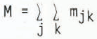. Because of sampling errors, the row totals of [D₁] may not be equal to those of [M]. Thus, a second matrix, [D₂], can be constructed in which

where 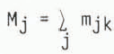. It is [D₂] which is used in testing the goodness of fit to the matrix of observed frequencies, [M]. A chisquared test is used which has one degree of freedom for a two-phase mosaic.

Illustrations

The technique is applied to two drumlin fields. One is the Vale of Eden field previously examined by Reference Smalley and UnwinSmalley and Unwin (1968) using nearest-neighbour analysis. The other is a field in the Dundalk area of southern Ontario.

Figure 2 reproduced from Reference Smalley and UnwinSmalley and Unwin (1968) shows the Vale of Eden field they examined. The drumlins in this pattern were identified from 1:25000 topographic maps by means of contour patterns (Reference Smalley and UnwinSmalley and Unwin, 1968, p. 387). Approximately 7% of the study area is covered by drumlins. This value was obtained by direct measurement but, if the researcher prefers to avoid this tedious task, made especially more so by large fields, the proportions can be estimated (Reference PielouPielou, [1975], p. 200). The pattern was sampled both parallel and perpendicular to the assumed ice flow, which was defined as the average azimuth of the orientation of the drumlins’ long axes (154°). Reference PielouPielou (1965, p. 912) suggested that the length of such a traverse should be short enough for there to be pronounced dependence between the points forming the pair and long enough for most of the m_jk (j ≠ k) to form an appreciable fraction of the total. Our choice of traverse lengths was guided by this observation and the lengths used are such that there is a non-zero chance that the points in a pair may fall within a single drumlin. This was achieved by setting the length of a traverse equal to one-half of the average length of the drumlins’ long axes (327 m) in the direction parallel to the assumed ice flow and at half that distance (163.5 m) perpendicular to the ice flow. Two sets of 150 points, each located at random in the study area, were then created. Each of these points was taken as the southernmost or westernmost point of a pair of points lying the specified distance apart in a direction of 154° or 244°. The states (i.e. drumlin or non-drumlin) at each end of these traverses were recorded and are given in Table I. Subsequent analysis, summarized in Table I, shows that both in directions parallel and perpendicular to assumed ice flow the sampled frequencies are not significantly different from those expected for a random mosaic with the same proportion of drumlinized area.

Fig. 2. Vale of Eden drumlin field analyzed by Reference Smalley and UnwinSmalley and Unwin (1968).

The other drumlin field examined is located in the Dundalk area of southern Ontario (see Fig. 3). This field has not been described previously in the literature. Drumlins were identified by stereoscopic interpretation of air photographs at a scale of 1:15840 followed by selective field checking. Initially, all features exhibiting some degree of elongation and positive local elevations were classified as drumlins. Subsequently, eskers and moraines were eliminated from the group. Approximately 6% of the study area is covered by drumlins. A part of this field is shown in Figure 4.

Fig. 3. Location of the Dundalk drumlin field (Canada. Dept. of Energy, Mines and Resources, 1972).

Fig. 4. A part of the Dundalk drumlin field.

As in the previous analysis, the pattern was analyzed both parallel and perpendicular to the assumed direction of ice flow. However, since the drumlins in this field show greater variation in their orientation than those in the first area, it was decided to perform two sets of analyses. In the first of these sets, the sampled directions were the mean drumlin azimuthal orientation (157°) and a direction orthogonal to this (247°), while in the second they were the modal orientation (135°) and 225°. In each case, the pattern was sampled using 150 short traverses. As in the previous illustration, the southern and western ends of the traverses were located at random in the study area and their lengths were equal to one-half of the average drumlin length (230 m) in the direction parallel to the assumed ice flow and one-quarter of the average drumlin length (115 m) in the direction perpendicular to the assumed ice flow. The resulting samples are shown in Tables II and III. For both directions, for both sets of analyses, the results again indicate that the pattern is not significantly different from a random mosaic.

Table I. Vale of Eden (a₁, a₂) (0.071, 0.929)

Table II. Dundalk Area, Mean Orientation (a₁, a₂) (0.063, 0.937)

Table III. Dundalk Area, Modal Orientation (a₁, a₂) (0.063, 0.937)

Concluding Comments

We have presented a method of analyzing the within-field spatial distribution of drumlins which we think is both more appropriate and useful than existing methods. However, this does not mean that the new method could not be refined. In particular, some might question the choice of the random-line mosaic as an appropriate general random mosaic model for drumlins. This model was chosen, in part, because of its availability and analytical tractability. Of course, the technique does not preclude the use of other models, such as the random placement model of Reference Smalley and UnwinSmalley and Unwin (1968), as the random mosaic model. However, it is unlikely that such alternative models will possess properties which are as easily identified and described as the Markovian ones of the random-line mosaic. In such circumstances, we will have to resort to the use of a simulation approach as, for example, Reference DiggleDiggle (1981) did in his study of patterns of heather as two-phase mosaics. In general, such an approach involves simulating the process believed to have been responsible for generating the empirical pattern and then using a Monte Carlo testing procedure. In summary, this would involve measuring one or more properties of the empirical pattern (P₂ would seem a likely choice) and considering this pattern as the outcome of the hypothesized process. This process is then simulated in order to obtain a number of patterns (usually 99 to correspond with conventional significance levels). The same property is then obtained for each of the simulated patterns. We can then examine where the value for the empirical pattern falls within the entire set of 100 values (99 from simulated patterns and one from the empirical), thus giving an indication of the likelihood of the empirical pattern occurring under the conditions of the hypothesized process. A more detailed discussion of this testing procedure has been given by Reference Diggle, Cormack and OrdDiggle (1979).

Finally, of course, the value of the method will be determined by its ability to enable us to ask and answer more pertinent questions about within-field drumlin distribution (Reference MenziesMenzies, 1979). To this end, we suggest that it would be valuable to use this method in future comparative studies of drumlins.