


1. INTRODUCTION
Sculpted formations such as sastrugi give visual clues to the nature of wind blowing over a snow surface yet the effects of ventilation beneath the snow surface remain poorly understood. Vetted theories describe how ventilation could potentially enhance sublimation from surface snow and also stimulate air movement at depth. For example, Albert (Reference Albert2002) modeled topographically induced snow ventilation in a megadunes site in Antarctica, simulating quasi-stationary pressure patterns and vapor flux that formed zones of preferential sublimation and deposition beneath the snow surface. In a wind tunnel experiment, Sokratov and Sato (Reference Sokratov and Sato2000) attributed airflow through the snow pore space to turbulence although others have cast doubt on the role of turbulence in producing interstitial air movement (Clifton and others, Reference Clifton, Manes, Ruedi, Guala and Lehning2008; Bartlett and others, Reference Bartlett and Lehning2011). More recently, Bowling and Massman (Reference Bowling and Massman2011) examined CO2 flux through seasonal snow cover and correlated enhanced diffusion of stable isotopes with windpumping, a process that can enhance gaseous transport through the snow when pressure changes occur faster than the in-snow air movement response. However, in a laboratory vapor diffusion study, Pinzer and others (Reference Pinzer, Schneebeli and Kaempfer2012) attributed sublimation and deposition rates across a snow sample to temperature gradients and suggested that wind-enhanced sublimation does not occur through a snow layer. Both Kawamura and others (Reference Kawamura2006) and Severinghaus and others (Reference Severinghaus2010) suggested that windpumping might account for deeper than expected convection zones in polar firn. Taken together, these studies suggest that pressure differences across several scales of motion spawn air movement in the snowpack but with a great degree of uncertainty in magnitude and effect.
When modeling in-snow response to ventilation Colbeck (Reference Colbeck1989; hereafter referred to as CB89) and Waddington and others (Reference Waddington, Cunningham and Harder1996: hereafter referred to as WD96) hypothesized an exponential decrease in perturbation pressure with depth, reaching zero amplitude at the lower boundary. These upper and lower boundary conditions constrain the modeled perturbation pressure field as well as the vertical profile of Darcian flow over the entire depth of the snowpack. In this paper, we test the CB89 and WD96 one-dimensional (1-D) models using field-based measurements in which we examine the degree to which wind-induced pressure perturbations attenuate with depth in snow. These results provide insights into how perturbation pressure energy is delivered to the snowpack, and they help constrain the depth within which ventilation can stimulate air movement within the snowpack.
2. METHOD
2.1. Site description
We performed in situ measurements of wind forcing and pressure response on Plaine Morte Glacier, Switzerland over the course of several weeks during early spring 2010. Plaine Morte Glacier is the largest plateau glacier in the European Alps (Huss and others, Reference Huss, Voinesco and Hoelzle2013) with an extent of ~5 km × 2 km and elevation, 2750 m. This site, part of the Crans-Montana ski area, has been used for several previous surface-atmosphere (Bou-Zeid and others, Reference Bou-Zeid, Higgins, Huwald, Meneveau and Parlange2010; Huwald and others, Reference Huwald2012) and hydrologic (Finger and others, Reference Finger2013) experiments. Seasonal snow typically overlies bare ice because net ablation in recent years has exhausted the firn layer. Plaine Morte Glacier is on average ~100 m thick, 15–20 m near the glacier edge and up to 200 m at its center. Over the 6-week course of the experiment, the seasonal snowpack ranged in depth from 3 to 4 m at the instrument site. Prevailing wind measurements acquired from a wind vane and cup anemometer over a 3-week period from late February through mid-March informed a deployment footprint. The upwind fetch had a generally smooth surface with a gently rising inclination of several degrees punctuated by a ridgeline roughly 2 km upwind (Fig. 1).

Fig. 1. Plaine Morte Glacier, Switzerland (courtesy Google Earth) labeled with the experiment site (star). The bold arrow points in the direction of the prevailing wind.
2.2. Measurement method
To capture in situ measurements of pressure perturbations at known depths in the snow we fabricated four 1 m long wedge-shaped snow ‘pickets’ into which we embedded fittings with 10–25 cm spacing (Fig. 2). To each fitting we permanently fixed silicone tubing that was strung along the picket center and out the top of the picket (Fig. 3). The other tubing end was attached to a differential pressure transducer each time a deployment was initiated. Elliot's (Reference Elliot1972) data and previous experience dictated the need for pressure transducers with fast response. Additionally, we required a pressure sensor that spanned a range of tens of Pascals with measurement precision better than 1 Pa. For this purpose we employed Setra™ Model 264 differential pressure transducers, designed to operate with an accuracy of 1% full scale at temperatures ranging from −18 °C to 65 °C. Full-scale differential pressure measurements from −25 to +25 Pa were output as voltages ranging from 0 to 5 VDC. Laboratory tests revealed thermal drift somewhat larger than the advertised value of 0.033% full scale °F−1 (=0.06% full scale °C−1), highlighting a need to perform in-field base calibration.

Fig. 2. Schematic diagram of snow picket showing the most commonly used port locations (cm) and pressure reference.
In all, 28 pressure transducers were mounted on aluminum rails and placed in a plastic storage container for protection from the elements during data acquisition, and to facilitate transport. The pressure transducers on pickets 1 and 2 had been used in a previous study and had experienced some wear. Results between the older and newer pressure sensors qualitatively agreed, but the data scatter was greater for the older sensors. We therefore used measurements from pickets 1 and 2 for qualitative assessment only.
Before placing the pickets into the snowpack, we vertically inserted a thin aluminum plate against two support pipes into the snow. Each picket was then placed vertically with the side opposite the tubing ports positioned firmly against the aluminum plate. This configuration maintained the picket's vertical orientation and provided torque to continuously press the slightly tapered picket face against the snow, thus minimizing the likelihood of air pockets forming around the picket perimeter during placement. Once the snow pickets were in place, we positioned a Campbell Scientific CSAT3 sonic anemometer ~30 cm above the snowpack surface with respect to the center of the measurement volume and in close proximity to the snow pickets to characterize the near-surface atmospheric turbulence (Fig. 3). This close proximity between the sonic anemometer and snow pickets was intended to maximize the coherence of turbulent structures detected by the sonic anemometer and pressure transducers. We acquired pressure transducer and sonic anemometer data at 10 Hz using a Campbell Scientific CR5000 data logger.

Fig. 3. Campbell Scientific CSAT3 sonic anemometer poised above four snow pickets (only picket tops are visible below the red arrows) during the 25 March deployment (case 3).
2.3. Reference pressure
A differential pressure transducer measures the pressure difference between two points. Thus, a common reference is a critical requirement to inter-compare values collected from differential pressure transducers. The Setra 264 pressure transducer has two ports, which we refer to as the ‘low’ or reference port and a ‘high’ or measurement port. The low port of each differential pressure transducer was attached to a single common reference. Pressure perturbations were measured as the pressure difference between the reference (low port) and the high port. An ideal common reference removes pressure perturbations at the low port of each pressure transducer, thereby establishing a shared baseline such that high-port pressure measurements may be directly compared amongst different pressure transducers. The common reference was constructed as a double-walled vessel filled with small, irregularly shaped pieces of high-density foam to dampen in-container velocity and pressure fluctuations. The low-port tubing passed into the inner vessel with one pinprick hole providing air passage between the inner vessel and the outer vessel and a second pinprick hole connecting the outer vessel with the environment to minimize high-frequency pressure changes while allowing for gradual, synoptic scale equilibration, which could otherwise easily exceed the full scale of the pressure transducers.
For each deployment the reference pressure chamber was placed in the same container as the logger, thus high-pass filtering free-atmospheric pressure changes. We measured the relaxation time constant for the pressure chamber in a laboratory environment to minimize noise due to turbulence. The relaxation time was measured by injecting a known volume of air (0.5 mL) through a 1 m long stainless steel capillary (to reduce heating) into the reference chamber port that would normally connect to the low port of the pressure transducers. We noted an exponential decay in pressure as the reference chamber responded to this imposed pressure perturbation. The relaxation time was taken as the time required for the measured pressure to decay to 0.37 (or e− 1) of the imposed pressure and was found to be 75 ± 5 s. This time frame is short enough to respond to synoptic changes yet long enough to resolve high-frequency pressure changes. We cannot resolve the magnitude of pressure changes with frequency on the order of or below the chamber relaxation time because the reference chamber will equilibrate over the time span of the fluctuation and synthetically dampen the measured response. Our setup is therefore tuned to measure high-frequency pressure responses. Changes to the relaxation time under changing environmental conditions were an unmeasured potential source of error.
3. RESULTS
3.1. Snow state
To determine snowpack structure, we excavated a snow pit down to no less than 1 m depth and horizontally within 10 m of the snow picket location in each pressure picket deployment. Snow pits were excavated after the snow pickets had been placed; the pressure data acquired during snow pit excavation were not used in this analysis. We acquired vertical profiles describing layering, crystal properties, temperature and density to characterize the snowpack. The time/height cross section in Figure 4 summarizes the evolution of derived intrinsic permeability from Shimizu's (Reference Shimizu1970) formula for the specific permeability ( $B_0 = 0.077 d_0^2 {\rm exp}{\kern 1pt} [ - 7.8\; \rho _{\rm s}^* ]$
, where d
0 is the grain diameter and
$B_0 = 0.077 d_0^2 {\rm exp}{\kern 1pt} [ - 7.8\; \rho _{\rm s}^* ]$
, where d
0 is the grain diameter and $\rho _{\rm s}^* $
is the specific gravity of snow with respect to ice) over the time range of case studies. From literature reviews we expected that intrinsic permeability empirically derived using Shimizu's formula would yield calculated values in the range, 10−8–10−10 m2. However, Shimizu's formula applied to our measurements gave permeability values down to 10−12 m2 in deeper, denser snow. Clearly, Shimizu's formula yielded systematically low permeability values as snow density increased with depth. As Shimizu (Reference Shimizu1970) and Albert and others (Reference Albert, Shultz and Perron2000) noted, the topology of the snow matrix evolves to a state that no longer complies with the fundamental assumption of packed spheres, rendering his formula inappropriate. To compare our results with the theoretical models of CB89 and WD96 we assume a constant intrinsic permeability of 10−9 m2, which was a representative near-surface value over the course of the experiment (bold isopleth in Fig. 4). We present this result to underscore the notion that intrinsic permeability varied substantially over small changes in space and time at our experiment site.
$\rho _{\rm s}^* $
is the specific gravity of snow with respect to ice) over the time range of case studies. From literature reviews we expected that intrinsic permeability empirically derived using Shimizu's formula would yield calculated values in the range, 10−8–10−10 m2. However, Shimizu's formula applied to our measurements gave permeability values down to 10−12 m2 in deeper, denser snow. Clearly, Shimizu's formula yielded systematically low permeability values as snow density increased with depth. As Shimizu (Reference Shimizu1970) and Albert and others (Reference Albert, Shultz and Perron2000) noted, the topology of the snow matrix evolves to a state that no longer complies with the fundamental assumption of packed spheres, rendering his formula inappropriate. To compare our results with the theoretical models of CB89 and WD96 we assume a constant intrinsic permeability of 10−9 m2, which was a representative near-surface value over the course of the experiment (bold isopleth in Fig. 4). We present this result to underscore the notion that intrinsic permeability varied substantially over small changes in space and time at our experiment site.

Fig. 4. Derived snow permeability time-depth slice in log10 units. Vertical dotted lines indicate the dates snow pits were measured. Snow permeability was derived from the Shimizu (Reference Shimizu1970) formula, based on measured grain size and snow density.
3.2. Deployments
Between 16 March and 17 April 2010 we deployed our snow picket/sonic anemometer system 12 times for periods ranging from 3 to 44 h. Given that site access was available only when the Crans-Montana ski lifts were operating, most data were acquired during times between when the ski area opened in the morning and when it closed for the day. Six of the 12 deployments passed quality control constraints for time and wind directional continuity. We required consistent data intervals to accurately compute high-frequency correlations and for spectral analysis. Therefore, we did not use data that would have necessitated gap filling. Wind direction continuity was required because the relative pressure systematically changed with attack angle on a given picket. For example, wind forcing and in-snow pressure response at 100 cm depth shown between midnight on 12 April and midnight on 13 April in Figure 5 indicate that relative pressure magnitude changed sign at noon when the wind direction changed from southeasterly to northerly. So when the wind direction varied substantially, we could not discriminate between the influence of wind speed and wind direction on the relative pressure measured within the snow. We further describe the objective criteria for wind direction selection later.

Fig. 5. Relative pressure at 1 m depth, wind speed and wind direction are plotted for 12–13 April to show the directional dependence of relative pressure. Vertical dotted lines bracket the noon time frame during which wind direction changed considerably and the pressure response was evident at 1 m depth in dense snow.
To facilitate references to particular deployments that met quality control constraints we define reference indices for the six deployments in Table 1.
Table 1. Case studies

3.3. Calibration
As noted earlier, the baseline voltage for each pressure transducer changed in a non-systematic stepwise manner at the initiation of each deployment when the pressure reference was engaged. Differences in hydrostatic pressure between the pressure reference and pressure measurements at difference depths in the snow also introduced a pressure offset. The baseline voltage was therefore defined such that measured pressure changes asymptote to zero with wind speed. The method of finding this baseline offset for each pressure transducer is delineated below in the section, ‘Stationary Pressure Response to Wind Forcing’. It could be argued that pressure changes will not be zero even at zero wind speed; however, this degree of precision is below the measurement capability of the pressure sensors used in this experiment.
3.4. Experimental error
At the end of the first deployments we dug out the snow pickets to inspect picket air intake ports for icing and to verify that there was minimal air space around each picket by which pressure signals could bypass the snow medium and pass directly from the atmosphere into the pressure transducer intake (Fig. 6). By correlating visual inspections with pressure measurements we determined that leakage around a picket was only an issue for near-surface ports (10 and 20 cm depth) in the later stage of longer deployments as snow melted, eroded or sublimated away from the picket face. This process manifested in the data as an apparent increase in perturbation pressure response to a given wind forcing and was thus marked as unreliable data. Icing of ports on the pickets was another source of experimental error. Snow could become impacted into a picket air intake port during placement, or an intake port could ice over during a data-acquisition period. In this event, the variance in pressure measurements from iced ports had very low correlation with wind speed changes and was easily identifiable. Snow impaction/icing was a common source of experimental error that reduced the quantity of high-quality data collected below 50 cm depth. For data collected at 10, 20, 30, 40, 50, 75 and 100 cm depths, corrupted data accounted for 5, 5, 0, 17, 33, 33 and 33% of the case data, respectively.

Fig. 6. Dug out pressure pickets (backside) on 11 April after a 2-day deployment with warm daytime temperatures showing snow loss around the top of the picket but no direct air exposure below ~20 cm.
3.5. Stationary pressure response to wind forcing
We refer to stationary pressure as the relative pressure field that developed in response to constant wind blowing over a barrier, and we distinguish it from the perturbation pressure, which is variability in the pressure field caused by variations in wind forcing. CB89 and Albert (Reference Albert2002) theorized that topographic features generate a stationary pressure field that drives near-surface circulations in snow. To confirm the presence of a stationary pressure field we first needed to calibrate the baseline pressure for each pressure sensor for all six case studies in Table 1 such that we could inter-compare results between the cases. Constant topographic forcing is simulated by flow distortion over 10 cm of exposed snow picket as shown in Figures 2 and 3. To maximize the forcing/response signal, we removed the directional dependence of stationary pressure amplitude by excluding data >5° from the prevailing wind direction. The wind direction relative to the picket face was not necessarily known to a precision of ±5°, so we derived the optimal wind direction by iteration, choosing the orientation that gave highest stationary pressure response to wind speed forcing.
Pressures were then bin-averaged in 0.25 m s−1 wind speed increments to determine a characteristic curve for each observation period defining the stationary pressure response to the wind forcing as well as the standard deviation, which defined the perturbation pressure response. Figure 7 shows an example of the underlying data and the resulting characteristic curve for 18 March.

Fig. 7. Pressure vs wind speed bin-averaged at 20 cm depth in 0.25 m s−1 increments for data within ±5° of the prevailing wind direction. The colorbar indicates the wind direction in (°).
Inspired by the quadratic relationship between pressure and velocity in Bernoulli's equation, we fit a quadratic curve to the data and also tried linear and exponential curve fits. The curve fit was used to extrapolate wind speed to the y-intercept. We found the R 2 value was maximized with an exponential fit when applying the constraint that relative pressure must be minimized at zero wind speed. Without this constraint a given quadratic fit could have a higher R 2 and also exhibit non-physical behavior that the relative pressure at zero wind speed could be greater than the relative pressure at non-zero wind speed. The difference between an exponential curve fit and a quadratic curve fit was typically small (<1 Pa), but was larger for cases for which the quadratic fit was poor. In subsequent analysis, we ignore results at the upper limit of the data range where we had insufficient data to resolve a characteristic curve.
Once the relative pressure at which wind speed asymptotes to zero was determined for all six cases, the y-intercept was subtracted from the y-coordinate (pressure) of the bin-averaged center points. This procedure defined a common origin and allowed us to overlay case results. A flowchart delineating steps in this procedure is shown in Figure 8. Wind speed vs stationary pressure for all the cases are compiled in Figure 9 revealing a similar pressure response curve for each case. The general trend is that of an exponential response at low wind speed, transitioning to a linear response at higher wind speed. Largest stationary pressures were typically found closer to the snowpack surface as can be seen by the 5 cm deep measurement in Figure 9. This is the only case with a 5 cm deep pressure measurement as for all other cases we acquired data at no less than 10 cm depth. Aggregating all cases, 1 min averaged wind speeds ranged up to 9 m s−1 with corresponding averaged pressure responses up to 11.5 Pa. With a 5 m s−1 wind forcing the average pressure response was 4 Pa, which was similar to the 5 Pa response Albert and others (Reference Albert2002) reported for 7 cm amplitude sastrugi. Since the magnitude of the pressure response to wind forcing depends on the shape and size of the topographic forcing we cannot directly compare our result with Albert's, other than to note an order of magnitude correspondence.

Fig. 8. Flowchart showing steps taken to extract stationary pressure from pressure measurements.

Fig. 9. Stationary pressure vs wind speed for pickets 3 and 4 at all depths and all cases. The difference in pressure response to wind forcing between all depths for a given case was small relative to the difference between cases because the snowpack differences between cases had a greater effect than snow depth for a given case. For a given case, the pressure response to wind forcing statistically decreased but rarely monotonically decreased. On 18 March the top measurement was at 5 cm rather than 10 cm and is indicated by an arrow.
3.6. Stationary pressure attenuation
Although the magnitude and shape of the stationary pressure field depends on the nature of the topographic forcing, attenuation of the pressure field with depth depends rather on the characteristics of the snow medium. For each case we determine stationary pressure attenuation by comparing the pressure magnitude near the surface with deeper measurements. The presence of attenuation was determined by subtracting stationary pressure magnitude at one depth from the measurement just above. We compiled this result for all cases in Figure 10, which shows that, on average, the stationary pressure field decreases by 0.15 Pa m−1 below 10 cm. Monotonically decreasing stationary pressure was not typical because large excursions from a monotonic profile were common. These excursions obscured the decrease in stationary pressure with depth that is less ambiguously represented by ranking the pressure measurements. An ensemble average of all the cases indicates that the ordered rank for stationary pressure did attenuate with depth, consistent with Colbeck's and Albert's models. This result persists if we exclude any one of the cases from the ensemble result. The pressure sensors that we used had inadequate dynamic range to capture much larger near-surface pressure changes. However, one can infer from case 2 (Table 1) for which we had measurements at 5 cm depth (Fig. 9) that topographically induced stationary pressure decreases most quickly near the air/snow interface and then attenuates more slowly with depth.

Fig. 10. Stationary pressure attenuation with depth for pickets 3 and 4 using the data shown in Figure 9.
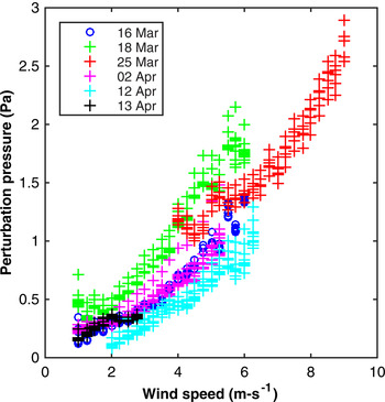
3.7. Perturbation pressure attenuation
We summarized the perturbation pressure energy given by the error bars in Figure 7 for each case in Figure 11, plotted against wind speed. Perturbation pressure increases superlinearly with wind speed. Rather than flattening out at high wind speed as seen for stationary pressure, the perturbation pressure curve maintains the same curvature at high values for all cases except case 6 (13 April in Fig. 11). For case 6 (Table 1), the perturbation pressure becomes less sensitive to wind speed as wind speed increases. Snow permeability at all depths was lowest for case 6, indicating that perturbation pressure is constrained in low permeability snow. We compared the arrival times of pressure perturbations at each depth by clipping out a 2 min (plus one data point) time period of 10 cm deep pressure data and a 1 min subset of pressure data from a deeper position and then sliding this subset index-by-index to find the position of best fit for the two signals as given by a Pearson correlation coefficient. The best alignment between the time series occurred with zero time offset indicating there was no distinguishable time delay between the 10 cm deep and deeper measurements. This result is expected because pressure perturbations propagate at the speed of sound and our data acquisition rate (10 Hz) was not fast enough to resolve the propagation characteristics of high-speed pressure fluctuations.
3.8. Spectral attenuation of perturbation pressure
As predicted by CB89 we find a spectral dependence of perturbation pressure attenuation within the snow wherein higher frequencies are more strongly attenuated with depth than are low frequencies. In Figure 12, we plotted pressure spectra for picket 3 in case 3, which is representative for surface snow with moderately high permeability. A spectral diagram shows the fractional contribution to variance by each frequency and is plotted in log form because power rapidly decreases with increasing frequency. This plot displays pressure energy over frequencies ranging from a fundamental frequency of 0.01 Hz, which is defined by the averaging time span, to the Nyquist frequency of 5 Hz, which is the highest resolvable frequency at a 10 Hz data acquisition rate. The data were initially subdivided into 30 min segments and 1024-point FFTs were then averaged. This averaged result represents a trade-off that improved signal-to-noise ratio at the expense of low-frequency resolution. The 1024 points acquired at 10 Hz corresponded to a 102.4 s averaging interval, which is slow enough for interstitial air movement to hydrostatically respond to pressure changes in a moderately permeable ~1 m deep snowpack. At the observed snow permeability and snow depth we capture the transition from a hydrostatic response to higher frequencies relevant to windpumping.

Fig. 12. Picket 3 perturbation-pressure spectra for case 3 (25 March) at depths given in the legend. In this case, high-frequency perturbation attenuated monotonically with depth to the noise floor at ~40 cm depth. The 95% confidence interval is displayed below the legend.
As shown in Figure 12, high-frequency pressure fluctuations are evident tens of centimeters deep in the snow. The spectra show that perturbation pressure energy decreases with depth in the snow down to 40 cm depth. Traces for the 40, 50 and 75 cm depths overlay each other and suggest a noise floor, meaning that high-frequency energy had dissipated by this depth. In most cases we observed aliasing of higher-frequency energy as well as evidence of a noise floor near the Nyquist frequency. For low permeability snow cases (not shown), differential spectral attenuation is nearly absent, presumably because high-frequencies had been attenuated in the 0–10 cm layer. For cases 1, 2, 4 and 6, the near-surface spectral slope (at 10 cm depth) was closer to the −7/3 value, predicted by the similarity theory, as in Bachelor (Reference Bachelor1951). For cases 3 and 5, the magnitude of the spectral slope was less and closer to −5/3, consistent with values predicted by Van Atta and Wyngaard (Reference Van Atta and Wyngaard1975). The decline in spectral slope at lower frequencies is likely because the relaxation timescale of the pressure reference was similar to the timescale of the pressure fluctuations, so the full magnitude of low-frequency pressure fluctuations was not captured. We did not find a systematic relationship that describes the dependency of spectral slope with other measured and derived parameters such as wind speed, turbulence intensity, atmospheric stability, surface snow density or permeability. We conclude that the perturbation pressure spectral slope also depends on snow characteristics for which we did not account, e.g. surface impedance, snow layering and tortuosity. That is, even with isotropic turbulence for which one might expect a −7/3 perturbation pressure spectral slope response, snow state may confound agreement between the measured and the expected spectral slope.
4. DISCUSSION
CB89 developed a theoretical solution that describes the attenuation of perturbation pressure with depth for a thin snowpack. WD96 found an analogous solution for an infinitely deep snowpack. Both of these solutions use the same form of perturbation pressure diffusivity, so we can compare our experimental results with these two theoretical results in that context. For both models the perturbation pressure diffusivity, κ p is:
 $$\kappa _{\rm p}{\rm \;} = {\rm \;} \displaystyle{{K\; P_0} \over {\mu \; \phi}}, $$
where K is the intrinsic permeability, P
0 is the atmospheric pressure, μ is the air viscosity and $ {\phi}$
is the snow porosity. From WD96, diffusivity forms the basis for a diffusion scale length,
$ {\phi}$
is the snow porosity. From WD96, diffusivity forms the basis for a diffusion scale length,
 $$H(\omega _0) = \; \sqrt {\displaystyle{{2\; \kappa _{\rm p}} \over {\omega _0}}}, $$
where ω 0 is the forcing frequency. The diffusion length scale can be thought of as the depth to which air can diffuse for a given frequency of wind forcing. As the forcing frequency decreases, air has more time to diffuse and can diffuse through a thicker snow layer.
Using the diffusion length as a scaling parameter we compare the theoretical prediction for the ratio of perturbation pressure throughout the snow depth (denoted as p) with the near-surface value (denoted p
0) from CB89 and WD96 with our experimentally derived values. Both theoretical solutions assume constant permeability so for comparison we use a 10–20 cm value of 10−9 m2, highlighted as a bold isopleth in Figure 4. We assume a constant snow porosity $ {\phi}$
= 0.65, with other constants μ = 1.65 × 10⁻⁴ Pl and P
0 = 9.75 × 10⁴ Pa, and h
0 = 3 m consistent with experimental values.
$ {\phi}$
= 0.65, with other constants μ = 1.65 × 10⁻⁴ Pl and P
0 = 9.75 × 10⁴ Pa, and h
0 = 3 m consistent with experimental values.
We investigate the instantaneous perturbation pressure power at two representative frequencies, 0.04 and 0.4 Hz, rather than the integral of the spectra (i.e. the variance) because the variability between cases at these frequencies is small thereby improving composite comparisons. These two frequencies bracket the 0.1 Hz frequency at which differential spectral attenuation typically increases (Fig. 12) and therefore represent solutions that bracket this kink point. We calculated attenuation with depth by dividing the instantaneous perturbation pressure at 10 cm from each deeper sensor. The experimental results show perturbation pressure attenuation with depth (box plots in Figs 13 and 14). If the 10 cm sensor were located closer to the surface we anticipate the near-surface pressure measurement would be larger and the resultant p/p 0 ratio would then be smaller at each depth. Our measurements show larger attenuation with depth than predicted by either WD96 or by CB89 yet our measurements under-predict near-surface perturbation pressure attenuation. We obtain an estimate of the surface-relative attenuation by calculating the surface perturbation pressure that would yield the observed attenuation as given by the comparison of perturbation pressure at 10 cm with deeper measurements. In both Figures 13 and 14, the thin dashed curve represents an exponential curve fit to the data with p 0 given by the perturbation pressure at 10 cm depth. We solve this curve fit for the perturbation pressure at 1 mm depth to obtain an estimate of the surface perturbation pressure:
 $$\displaystyle{z \over H} = a\exp \left( {b\; \displaystyle{{\,p_0} \over {\,p_{10}}}} \right)\; \to \; p_0 = \displaystyle{{\,p_{10}} \over b}\ln \left( {\displaystyle{z \over {Ha}}} \right).$$

Fig. 13. Measured and theoretical perturbation-pressure attenuation with depth at 0.04 Hz with depth scaled by the diffusion length scale. The horizontal axis is the perturbation pressure at a given depth divided by the reference (surface) perturbation pressure. The vertical axis is the depth divided by the diffusion length scale. The long-dashed curve shows measured perturbation pressure attenuation with depth using the 10 cm pressure as the reference pressure, p 0. The solid curve shows the attenuation calculated by extrapolating the tendency given by the long-dashed curve to the surface in order to determine a surface value for the reference pressure, p 0.

We then recomputed the attenuation using this surface estimate to obtain the fit plotted as the solid curve in Figures 13 and 14. At 0.04 Hz, an exponential curve fit of the form a × exp(b × p/p 0) gives coefficients a = −44.8 and b = −13.8. At 0.4 Hz, an exponential curve fit of the form a × exp(b × p/p 0) gives coefficients a = −0.11 and b = −6.63.
The primary cause of variability in the ratio p/p 10 between cases is not clear although we can discriminate several relevant parameters that are not the cause. For a given case, even large differences in density and intrinsic permeability with depth do not translate into large differences in perturbation pressure as seen by comparing Figure 4 with Figure 11. Likewise, wind turbulence spectra (not shown) do not indicate significantly different forcing that would lead to very different p/p 10 ratios between cases. We suspect that the differences in snow state other than density and intrinsic permeability such as surface hardness, tortuosity (microphysical structure) and layering account for much of the variability in p/p 10 ratio between cases. For example, a thin, low-permeability surface crust could inhibit turbulent energy and perturbation pressure transfer into the snowpack. In this instance, perturbation pressure entering the snowpack would be less than expected for a given bulk snow permeability and surface forcing.
An alternate analysis of pressure spectra presented by Clarke and Waddington (Reference Clarke and Waddington1991) supports this conclusion. The authors interpreted the difference in spectral magnitude between the surface and 10 cm deep pressure measurements as being due only to absorption by the snow medium. In the 10 cm pressure spectra, the spectral slope of the deeper measurement is close to −7/3, whereas the spectral slope of the surface measurement is close to −1, suggesting that the near-surface pressure spectra capture dynamic pressure changes of airflow around the pressure sensor rather than an unfettered cascade of turbulently generated perturbation pressure. An alternate interpretation of their results is that a significant portion of the energy difference between the surface and 10 cm depth measurements is due to scattering at the snow surface rather than solely due to attenuation through the snow layer.
In Figure 14, we show theoretical and measured attenuation at 0.4 Hz, a frequency within the range of differential attenuation for all the cases. Since the diffusion length scale is inversely proportional to the forcing frequency, both theories predict greater attenuation at higher frequencies relative to lower frequencies, but both theories still under-predict the observed attenuation. The experimental result is that high-frequency pressure perturbation is strongly attenuated with depth. Using a 3-D model Clarke and Waddington (Reference Clarke and Waddington1991) found that vertical perturbation pressure attenuation was enhanced by horizontal airflow when the surface forcing was spatially limited. Since the exposed portion of the snow pickets in our experiment generated a spatially limited pressure field our experimental result qualitatively agrees with their theoretical result. From the pressure spectra in Figure 12 it is clear that a small fraction of perturbation pressure energy resides at high frequencies, so strong attenuation of high-frequency pressure energy has a vanishingly small impact on spectrally integrated attenuation with depth (i.e. the variance). Measured attenuation exceeds model predicted attenuation even if we assume an unreasonably low uniform snow permeability (e.g. 10−11 m2, not shown) with a corresponding decrease in the e-folding depth.
5. CONCLUSIONS
We observed the relationship between wind and pressure at a data acquisition frequency of 10 Hz in an alpine snowpack to 1 m depth. The stationary pressure field that was formed by wind blowing over the exposed top 10 cm of a snow picket decreases with depth, consistent with Colbeck (Reference Colbeck1989) and Albert (Reference Albert2002). Since the stationary pressure field in our experiment was synthetic and because the shape of the stationary pressure field depends on the shape of the topographic feature, we broadly characterize this verification as order-of-magnitude agreement.
The thrust of this experiment was to separate stationary pressure from the perturbation pressure field, so that we could assess the relationship between wind forcing and the vertical profile of perturbation pressure in snow. We have documented perturbation pressure attenuation with depth at high frequencies and derived empirical formulas to deterministically calculate the average perturbation pressure attenuation at two representative frequencies, 0.04 and 0.4 Hz. At both these high frequencies the perturbation pressure field attenuated faster with depth than predicted by either Colbeck (Reference Colbeck1989) or Waddington and others (Reference Waddington, Cunningham and Harder1996). The perturbation pressure attenuation difference between theory and measurement increased with frequency. This result agrees with the Clarke and Waddington (Reference Clarke and Waddington1991) result that found enhanced perturbation pressure attenuation when the surface forcing was spatially limited. In turn, this agreement underscores the importance of simulating windpumping as a 3-D process.
Since frequencies above 0.04 Hz contain a small fraction of the total spectral energy of the perturbation pressure field, attenuation at these high frequencies negligibly decreases the spectrally integrated pressure energy within 1 m of snow depth. Continuity in this trend towards lower frequencies suggests that attenuation decreases with decreasing frequency, but remains greater than predicted by either of the two 1-D models considered in this paper. Although the fraction of perturbation pressure energy at high frequencies is small, differential spectral attenuation at high frequencies represents a signature that could be used to characterize the depth in snow that is perturbed by high-frequency turbulence. The lack of a robust similarity relationship between wind properties, perturbation pressure and permeability suggests that other parameters such as tortuosity, snow surface hardness and layering strongly affect perturbation pressure attenuation in snow. Explicit characterization of perturbation pressure energy for energy-rich lower frequencies remains a topic for future work.
ACKNOWLEDGEMENTS
This research was funded by the Laboratory of Environmental Fluid Mechanics and Hydrology at École Polytechnique Fédérale de Lausanne and the Landolt et Cie Endowed Chair for Sustainable Futures, Switzerland. Crans-Montana ski area provided key logistical support during the field campaign. We thank V. Piovano for measuring the relaxation time constant of the pressure reference and D. Chelton for guidance on the spectral error assessment. We are grateful to E.D. Waddington and an anonymous reviewer for providing constructive comments that greatly improved the paper.


 Open access